Obscured and unobscured AGN populations in a hard-X-ray selected sample of the XMDS survey

Abstract

Aims. Our goal is to probe the populations of obscured and unobscured AGN investigating their optical-IR and X-ray properties as a function of X-ray flux, luminosity and redshift within a hard X-ray selected sample with wide multiwavelength coverage.

Methods. We selected a sample of 136 X-ray sources detected at a significance of $\geq 3\sigma$ in the $2-10$ keV band ($F_{2-10}\ga 10^{-14}$ erg cm^-2 s^-1) in a $\sim 1$ deg² area in the XMM Medium Deep Survey (XMDS). The XMDS area is covered with optical photometry from the VVDS and CFHTLS surveys and infrared Spitzer data from the SWIRE survey. Based on the X-ray luminosity and X-ray to optical ratio, 132 sources are likely AGN, of which 122 have unambiguous optical - IR identification. The observed optical and IR spectral energy distributions of all identified sources are fitted with AGN/galaxy templates in order to classify them and compute photometric redshifts. X-ray spectral analysis is performed individually for sources with a sufficient number of counts and using a stacking technique for subsamples of sources at different flux levels. Hardness ratios are used to estimate X-ray absorption in individual weak sources.

Results. 70% of the AGN are fitted by a type 2 AGN or a star forming galaxy template. We group them together in a single class of “optically obscured” AGN. These have “red” optical colors and in about 60% of cases show significant X-ray absorption (N${}_{H}>10^{22}$ cm^-2). Sources with SEDs typical of type 1 AGN have “blue” optical colors and exhibit X-ray absorption in about 30% of cases. The stacked X-ray spectrum of obscured AGN is flatter than that of type 1 AGN and has an average spectral slope of $\Gamma=1.6$. The subsample of objects fitted by a star forming galaxy template has an even harder stacked spectrum, with $\Gamma\sim 1.2-1.3$. The obscured fraction is larger at lower fluxes, lower redshifts and lower luminosities. X-ray absorption is less common than “optical” obscuration and its incidence is nearly constant with redshift and luminosity. This implies that at high luminosities X-ray absorption is not necessarily related to optical obscuration. The estimated surface densities of obscured, unobscured AGN and type 2 QSOs are respectively 138, 59 and 35 deg^-2 at $F>10^{-14}$ erg cm^-2 s^-1.

1 Introduction

One of the goals of deep X-ray surveys is to probe the origin of the X-ray background (XRB) to the faintest flux levels; they have resolved into discrete sources more than 90% of the XRB in the $0.5-2$ keV band and up to 80 - 90% in the $2-10$ keV band (Giacconi et al., 2002; Alexander et al., 2003; Moretti et al., 2003; De Luca & Molendi, 2004). The resolved fraction of the XRB drops however to $\sim 60$% above $\sim 6$ keV and $\sim 50$% above $\sim 8$ keV (Worsley et al., 2005). Most of the sources detected in deep, pencil-beam X-ray surveys are characterized by poor counting statistics, preventing a detailed analysis of X-ray spectral properties, and optical counterparts are often too faint for spectroscopic follow-up. Medium deep surveys, covering larger areas, are useful to bridge the gap between known X-ray source populations at low redshifts and those required to model the background and to collect a large number of sources for which X-ray and optical spectral analysis are feasible (e.g. Piconcelli et al., 2003; Georgakakis et al., 2006). They are also more effective than deep surveys to find rare objects, such as type 2 QSOs (Fiore et al., 2003).

The XMM Medium Deep Survey (XMDS, see Chiappetti et al., 2005, hereafter Paper I) consists of 19 X-ray pointings, of nominal exposure of 20 ksec, covering a contiguous area of about 2.6 deg². It also lies at the heart of the larger, shallower XMM Large Scale Structure (LSS) Survey (Pierre et al., 2004; Pacaud et al., 2006), which will cover $\sim 10$ deg² and is principally devoted to clusters study (Pierre et al., 2006). Several surveys at different wavelengths are associated to the XMDS: the VIRMOS VLT Deep Survey (VVDS, Le Fèvre et al., 2004) and the Canada - France - Hawaii Telescope Legacy Survey (CFHTLS) in the optical, the UKIRT Infrared Deep Sky Survey (UKIDSS, Dye et al., 2006; Lawrence et al., 2006) in the near-IR and the Spitzer Wide-Area InfraRed Extragalactic Legacy Survey (SWIRE, Lonsdale et al., 2003) in the mid-IR. Radio observations performed at VLA at 1.4 GHz (Bondi et al., 2003) and at 325 and 74 MHz (Cohen et al., 2003) also cover the XMDS area.

In Paper I the catalogue of XMDS sources detected ($S/N\geq 4\sigma$) in at least one of five energy bands $0.3-0.5$, $0.5-2$, $2-4.5$, $4.5-10$ and $2-10$ keV within the VVDS field (area $\sim 1$ deg²) was presented together with tentative optical identifications. The logN-logS distributions were derived for X-ray sources in the full XMDS area separately in the two bands $0.5-2$ and $2-10$ keV. Gandhi et al. (2006) computed the logN-logS in the same energy bands for X-ray sources in the whole XMM - LSS area, finding results in agreement with those of Paper I.

Here we consider a sample of X-ray sources selected in the “hard”, $2-10$ keV, band, in order to investigate the populations of obscured and unobscured AGN and discuss their multiwavelength properties in a way unbiased by the intensity of the sources in soft X-rays. In order to take advantage of the best multifrequency coverage available, we consider sources in the VVDS area. Using the Spitzer data we construct the mid-IR/optical to X-ray spectral energy distributions (SEDs) of the sources to estimate redshifts and classify AGN into different categories according to the best fitting template. We use the term “optically unobscured” AGN for objects fitted by a type 1 AGN template, and “optically obscured” AGN for objects fitted by type 2 AGN or a star forming galaxy template, indicating that the optical-UV emission from the AGN is at least partially hidden. In a companion paper (Polletta et al., 2007) the templates used and the observed SEDs are presented in detail and their dependence on luminosity and absorption is discussed. A comparison between X-ray and optical properties of AGN with optical spectroscopy in the whole XMM-LSS is in progress (Garcet et al., in prep.).

Independently of the SED classification, the X-ray spectra and/or hardness ratios allow us to estimate absorption in the X-ray band, associated to intervening gas. In unified models for AGN (e.g. Antonucci, 1993), obscuration by dust and absorption by gas are thought to occur in a dusty torus surrounding the AGN. The increasing complexity of properties shown by individual AGN has lead to a revision of this simple scheme proposing different regions around the AGN as sites of absorption at different wavelengths (e.g. Elvis, 2000; Krongold et al., 2007; Elitzur, 2006). We will therefore distinguish optically obscured and X-ray absorbed AGN and examine separately their dependence on X-ray flux, redshift and luminosity.

The paper is organized as follows: the multiwavelength data set is presented in Section 2. Optical and IR identifications are discussed in Section 3 while the X-ray, optical and IR properties of the sample are derived in Section 4. The template SEDs and fitting process leading to the estimate of photometric redshifts and to the AGN classification are described in Section 5. The X-ray spectral analysis is presented in Section 6: X-ray spectra are analyzed individually for sufficiently bright sources, while for faint sources absorption is estimated from hardness ratios. A stacking technique is used to derive average X-ray spectra of subsamples of AGN with different SED classification. The surface density of optically obscured and unobscured AGN and of type 2 QSOs is derived in Section 7. Section 8 is devoted to the comparison of the fractions of optically obscured or X-ray absorbed AGN as a function of redshift, X-ray flux and luminosity. Finally, in Section 9 the results are summarized.

Throughout the paper H${}_{0}=70$ Km s^-1 Mpc^-1, $\Omega_{\Lambda}=0.7$ and $\Omega_{M}=0.3$ are assumed.

2 The multiwavelength data set

Figure 1: Layout of the 19 XMM - Newton pointings of the XMDS (circles; the dashed circle marks field G12, which was not analyzed because of high background level, see Paper I) and of the associated surveys: VVDS (solid rectangle), CFHTLS Deep (D1, short dashed rectangle), and Wide (W1, area on the right side of the vertical solid line), UKIDSS (long dashed rectangle) and SWIRE (area on the right side of the diagonal solid line).

The layout of the XMDS observations is shown in Fig. 1; superposed are the areas covered by the various associated surveys at other wavelengths, VVDS and CFHTLS in the optical, UKIDSS in the near-infrared and SWIRE in the mid-infrared. Shallower XMM - Newton pointings in the context of the XMM - LSS lie all around the XMDS area (see Pierre et al., in prep.)

2.1 X-ray data

The sample includes 136 X-ray sources detected at $\geq 3\sigma$ in the $2-10$ keV band (the 3 $\sigma$ hard sample hereafter), which fall within the sky area covered by the VVDS photometric survey ($\sim 1$ deg², solid rectangle in Fig. 1). This area benefits from the richest multiwavelength coverage as evident from Fig. 1.

The sources were extracted from the XMDS catalog described in Paper I, to which we refer also for details on the XMM - Newton observations and data reduction. For all the sources count rates and fluxes were obtained independently in 5 energy bands: $0.3-0.5$, $0.5-2$, $2-4.5$, $4.5-10$ and $2-10$ keV. Fluxes were computed for a simple power law spectrum with spectral index $\Gamma=1.7$ and the average galactic column density in the XMDS region (N${}_{H}=2.61\times 10^{20}$ cm^-2, Dickey & Lockman, 1990) separately in each energy band. Fig. 2 shows the $2-10$ keV flux distribution; the lowest flux that we sample is $\sim 10^{-14}$ erg cm^-2 s^-1.

Hardness ratios were computed for all sources (see subsection 6.2). For 55 sources we detect a sufficient number of net counts $(>50$ in the $2-10$ keV band) to attempt a spectral analysis for each source (see details in subsection 6.1).

Figure 2: 2 - 10 keV flux distribution for the 136 X-ray sources in the 3 $\sigma$ hard sample.

2.2 Optical and near-infrared data

Broad band BVRI photometric observations from the VVDS (McCracken et al., 2003) are available for XMDS sources over an area of about 1 deg². This photometry was obtained at the Canada France Hawaii Telescope (CFHT) with the CFH12K camera at limiting magnitudes of $B_{AB}\sim 26.5,V_{AB}\sim 26.2,R_{AB}\sim 25.9$ and $I_{AB}\sim 25.0$ (50% completeness for point sources).

The U band imaging was performed over an effective area of $\sim 0.71$ deg² with the Wide Field Imaging (WFI) mosaic camera on the ESO MPI 2.2 m telescope at La Silla, Chile. Two different U filters were used, the ESO U/360 filter and the Loiano Observatory U filter. The limiting magnitude is $U_{AB}\sim 25.4$ (see Radovich et al., 2004).

A small area ($\sim 165$ arcmin²) within the VVDS was also observed in the J and K bands down to a limiting magnitude of $J_{AB}\sim 24.2$ and $K_{AB}\sim 23.9$ (50% completeness for point sources) with the SOFI instrument mounted on the ESO NTT telescope. A detailed description of the $K$ band imaging survey is reported in Iovino et al. (2005).

Optical spectroscopy with the VIsible Multi Object Spectrograph (VIMOS) on the ESO – VLT UT3 in the VVDS area is still in progress; the project aims at observing a representative large subsample of objects down to a limiting mag of $I_{AB}\leq 24$ (Le Fèvre et al., 2005). 9 sources in the present sample have been observed and for 8 of them a redshift has been derived. Additional spectroscopic redshifts for 22 sources have recently been obtained from 2dF and VLT FORS2 observations performed in the context of XMM-LSS follow up campaigns (see Garcet et al., in prep.). Three other redshifts are from the literature.

The XMDS area lies within the sky region covered by the CFHTLS, a large collaborative project between the Canadian and French communities. Observations use the wide field imager MegaPrime equipped with MegaCam, in the $u^{*}g^{\prime}r^{\prime}i^{\prime}z^{\prime}$ filters. Both the “Wide” survey field W1 (8 deg $\times$ 9 deg) and the “Deep” survey field D1 (1 deg $\times$ 1 deg) cover the XMDS region at a depth of $i^{\prime}=24.5$ (Hoekstra et al., 2006) and $i^{\prime}=26.1$ (50% completeness limit, Semboloni et al., 2006), respectively. In the following we will use the D1 notation for data from the CFHTLS Deep and the W1 notation for data from the CFHTLS Wide. W1 observations have been recently completed; the coverage shown in Fig 1 is deduced from data available to us at the time of analysis.

Near-infrared observations of the XMDS area are also in progress in the context of the UKIDSS (Dye et al., 2006; Lawrence et al., 2006). The survey uses the Wide Field Camera (WFCAM) of the 3.8 m United Kingdom Infrared Telescope (UKIRT). The XMM-LSS region is one of the four target fields of the Deep Extragalactic Survey (DXS). Observations in the $J$ and $K$ filters down to $J=22.3$ and $K=20.8$ (Vega system) are in progress. About 0.8 deg² of sky have been observed up to now and part of the data are available in the UKIDSS Early Data Release (Dye et al., 2006). The photometric system used in the UKIDSS is described in Hewett et al. (2006).

2.3 Mid-infrared data

The XMDS and XMM-LSS fields are covered by the SWIRE survey (Lonsdale et al., 2003). Observations were performed with the Infrared Array Camera (IRAC) at 3.6, 4.5, 5.8 and 8.0 $\mu$m and with the Multiband Imaging Photometer (MIPS) at 24, 70 and 160 $\mu$m to a $5\sigma$ depth of 4.3, 8.3, 58.5, 65.7 $\mu$Jy and 0.24, 15, and 90 mJy, respectively. The area covered in the XMDS region is about 2.5 deg², corresponding to about 95% of the field. 12 sources in our selected sample are outside the region covered by SWIRE. Details on the SWIRE data and source catalogs are given in Surace et al. (2005).

2.4 Radio data

There are also radio observations associated with the XMDS: the VLA VIRMOS Survey, which covers the VVDS area at a depth of 80 $\mu$Jy ($5\sigma$ limit) and a resolution of 6″ at 1.4 GHz (Bondi et al., 2003; Ciliegi et al., 2005) and a low frequency radio survey performed for the XMM-LSS also at VLA, which covers 5.6 deg² at a depth of 4 mJy at 74 MHz and 110 deg² at a depth of 275 mJy at 325 MHz (Cohen et al., 2003).

3 Optical and Infrared identifications

Most (80%) of the 136 X-ray sources in the present sample were already included in the $4\sigma$ catalogue presented in Paper I since they are also detected at $\geq 4\sigma$ in the softer bands. 24 X-ray sources are considered here for the first time. Although most sources had already been assigned optical counterparts, we have repeated the identification procedure on the whole sample in a semi automatic way, that takes into account the experience accumulated in Paper I and the CFHTLS and SWIRE data now available.

Access to the whole VVDS and CFHTLS catalogues and images is restricted: photometric data and positions are provided only for optical sources within a fixed radius from the X-ray positions. The same is true for the SWIRE data. We then associated to each X-ray source all combinations of optical and IR objects in the considered catalogues within a search radius of 6″. Objects in the VVDS, CFHTLS and SWIRE catalogues were matched only a posteriori.

We computed the probability of chance coincidence between an X-ray source and all optical VVDS, optical CFHTLS and infrared SWIRE candidates within the search radius using the following equation (Downes et al., 1986, see also Paper I)

$$p=1-exp(-\pi\leavevmode\nobreak\ n(<m)\leavevmode\nobreak\ r^{2})$$

where $r$ is the distance between the X-ray source and the proposed counterpart (with a lower value fixed at 2″, which roughly corresponds to the XMM - Newton astrometric uncertainty), and $n(<m)$ is the density of objects brighter than the magnitude $m$ of the candidate counterpart. We used $I$ magnitudes for VVDS sources and $i^{\prime}$ magnitudes for CFHTLS objects (D1 data where available). We used the density $n(>F_{3.6})$ for infrared candidate counterparts. For each candidate counterpart there are therefore from 1 to 3 values of $p$, depending if the object is detected in the VVDS, CFHTLS and SWIRE. We classified the probabilities as “good” ($p<0.01$), “fair” ($0.01<p<0.03$) or otherwise “bad” and took as identification the object with the best probability combination. All tentative identifications were then checked by visual inspection using the VVDS finding charts. As reported in Paper I, astrometrical corrections were already applied to the X-ray fields, so we find again that 98% of the counterparts are within 4″ from the X-ray corrected position, justifying our conservative choice of 6″ radius.

The probability criterion allows us to prefer one candidate counterpart in the majority of cases, giving us 126 secure identifications (out of 136 sources). Of these, 3 have only IR counterparts (i.e. no optical counterparts are detected down to $R_{AB}=25.3$) and will be referred to as optically blank fields. We notice that all sources covered by SWIRE (i.e. all but 12) are also detected in the IR.

For the remaining 10 sources, the identification process is ambiguous leaving two or more possible counterparts, with similar probabilities. However, in 6 cases, the counterparts have similar magnitudes and colors allowing us to include these sources in parts of the discussion not involving the redshift determination or SED classification. In the other 4 cases, the sources are completely dismissed.

The X-ray, optical and infrared properties of sources of the 3 $\sigma$ hard sample are reported in Table A. For brevity, not all data used in this work are reported in the Table. The SWIRE catalogue is available through IRSA/Gator (http://irsa.ipac.caltech.edu/applications/Gator). We plan to publish the Catalogue of all XMDS X-ray sources with optical and IR identifications in a future paper.

We also searched for UKIDSS counterparts of X-ray sources using a radius of 4″, finding a near infrared counterpart for 72 X-ray sources. Generally UKIDSS sources are coincident with optical counterparts. There are however two exceptions: source XMDS 449 for which the UKIDSS source lies between the two possible counterparts, at a distance of about 3″ from both, and XMDS 760, for which there are two possible UKIDSS counterparts, both within $\sim 1$″ from the optical counterpart. The first case is one of the 4 X-ray sources that we could not identify, and the UKIDSS detection did not allow us to resolve the ambiguity. In the second case we associated to the optical counterpart the brightest UKIDSS source.

33 X-ray sources in the $3\sigma$ hard sample (24%) have a radio counterpart at 1.4 GHz, one of them is also detected at 325 MHz. One is however associated with the spectroscopically confirmed cluster XLSSC 025. We will not use the radio information in this work, but we checked the consistency of the radio fluxes with the templates used to fit the optical and infrared spectral energy distributions of our objects (see Section 5). The correlation between the X-ray and radio luminosities is explored in Polletta et al. (2007).

4 The AGN sample

Figure 3: X-ray to optical ratio ($2-10$ keV band vs $R$ band) as a function of X-ray flux for sources in the 3 $\sigma$ hard sample. Diagonal dotted lines indicate loci of constant $R$ magnitude while horizontal solid lines mark the region of canonical AGN ($0.1<F_{X}/F_{R}<10$). Lower limits mark the optically blank fields, whose $R$ magnitude was fixed to 25.3 (see Fig. 13 in McCracken et al., 2003).

Ignoring two sources corresponding to spectroscopically confirmed galaxy clusters (XLSSC 025 and 041, see Pierre et al., 2006), we computed the X-ray to optical ratio for 124 sources with secure identifications, using the equation given in section 6.2 of Paper I. For about 20 objects for which VVDS magnitudes were unreliable because of saturation or unfavorable position in the field of view, the CFHTLS $r^{\prime}$ band magnitudes were used, with the appropriate conversion factor taken from Silverman et al. (2005). The X-ray to optical ratio is shown as a function of X-ray flux in Fig. 3.

About 80% of the sources fall in the typical range of X-ray to optical ratio corresponding to the locus of AGN ($0.1<F_{X}/F_{R}<10$, see e.g. Akiyama et al., 2000; Hornschemeier et al., 2001), while about 20% of the sources have $F_{X}/F_{R}>10$, which corresponds to heavy absorption in the optical and/or high redshift (Hornschemeier et al., 2001). This issue will be further developed in subsection 7.1.

Only two sources fall significantly below the AGN borderline (XMDS 1248 and 842): both appear extended in the optical as well as in the infrared images. The first (XMDS 1248) has a low hardness ratio, consistent with no intrinsic absorption in the X-ray spectrum, while the second (XMDS 842) has a higher hardness ratio, possibly indicating X-ray absorption (N${}_{H}\sim 10^{22}$ cm^-2). Using photometric redshifts (see Section 5), we obtained X-ray luminosities of $\sim 10^{41}$ erg s^-1 for both of them, even after correcting for absorption (see Table A). We classify both provisionally as normal galaxies, though we can not exclude the presence of a low luminosity AGN or even a Compton thick AGN in XMDS 842 (see e.g. FSC 1021+4724 in Alexander et al., 2005). Another source in the sample has $L_{0.5-10}<10^{42}$ erg s^-1, XMDS 178, however its X-ray to optical ratio of 0.27 is in the typical AGN range. On the basis of the X-ray to optical ratio, we retain this source in the AGN class. In Polletta et al. (2007) slightly different criteria are adopted for these borderline objects.

To summarize, on the basis of the X-ray to optical flux ratios 122 X-ray sources with unambiguous identification can be classified as AGN and 2 as normal galaxies. In the following subsections we will discuss the optical and IR properties of this sample.

4.1 Optical magnitude and colors

Figure 4: $B-I$ distribution for optical counterparts of X-ray sources in the 3 $\sigma$ hard sample. The dotted line marks the division between the adopted definition of “blue” and “red” objects (see text).

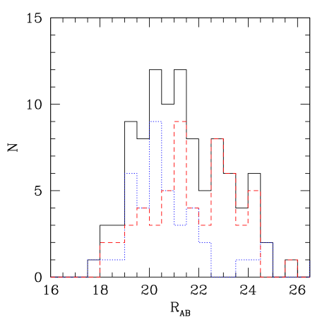
Figure 5: $R$ magnitude distribution for the 3 $\sigma$ hard sample. Solid histogram: total sample; dotted histogram: blue sources (see text); dashed histogram: red sources (see text).

The $B-I$ color and the $R_{AB}$ magnitude distributions for the identified sources are shown in Fig.  4 and 5, respectively.

The $B-I$ color distribution shows a high peak at $B-I\leq 1.0$, and a tail extending up to $B-I\sim 4$. Based on the observed color distribution we adopt a somewhat arbitrary threshold of $B-I=1.0$ to divide the sample into two roughly equal size samples of “blue” objects, with $B-I<1.0$ (43% of all sources), and “red” objects, with $B-I>1.0$ (57%). As will be shown later, this criterion, although crude, proved to be a good one for a rough separation between type 1 (i.e. broad line) AGN and type 2 (narrow line) or star forming galaxy-like AGN based on observed quantities alone, and is substantially confirmed by the more detailed (but model-dependent) classification based on the spectral energy distributions.

The magnitude distributions of these two broad classes are plotted separately in Fig. 5: on average, blue sources ($B-I\leq 1.0$) are brighter, with a peak at $R\sim 20$ and 90% of objects at $R<22$, while red sources ($B-I>1.0$) have a broader distribution, extending from $R\sim 18$ to $R\sim 26$.

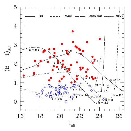
Figure 6: $B-I$ color vs $I$ magnitude for sources in the 3 $\sigma$ hard sample. Empty circles are blue objects, filled circles are red objects. Overimposed to points are the evolutionary tracks for an Sc galaxy (solid line), a type 1 QSO (dotted line), a type 2 AGN (short-dashed line) and a type 2 AGN plus a starburst component (long-dashed line). The B band absolute magnitudes assumed are $-15.7$ for the Sc galaxy template, $-22.3$ for the QSO1, $-16.9$ for the type 2 AGN and $-23.9$ for the type AGN plus starburst.

In Fig. 6 we show the $B-I$ color as a function of the $I$ magnitude for our sources, along with the evolutionary tracks for various templates: a late spiral galaxy (Sc, solid line), a type 1 QSO (dotted line), a type 2 AGN (short-dashed line) and a type 2 AGN plus a starburst component (long-dashed line; see below and Polletta et al., 2007). The effects of absorption due to the Intergalactic Medium (IGM) have been taken into account at high redshift ($z\geq 2.5$) as prescribed in Madau (1995). Blue sources are near the QSO1 track, while red objects are generally consistent with star forming galaxies and AGN2 tracks. However for magnitudes fainter than $I_{AB}=23$ the different track cross, and type 1 AGN, type 2 AGN and star forming galaxies have similar colors.

4.2 X-ray to infrared ratios

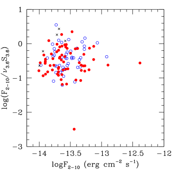
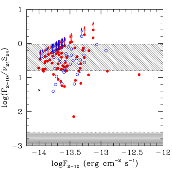
Figure 7: X-ray to IR ratio as a function of X-ray flux for sources in the $3\sigma$ hard sample. Empty circles are blue sources, filled circles are red sources, crosses are the optically blank fields or sources with undefined color classification (because $B$ or $I$ magnitudes are not available). In the left panel IRAC 3.6 $\mu$m flux is used, while in the right panel MIPS 24 $\mu$m is used. Lower limits are sources detected in one or more IRAC bands and undetected in the MIPS 24 $\mu$m band, where 5 $\sigma$ upper limit is used. The diagonally shaded area is the region occupied by hard X-ray selected AGN with IR emission and $z<0.12$ from Piccinotti et al. (1982); the horizontally shaded area is the region occupied by local starburst galaxies from Ranalli et al. (2003).

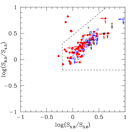
Figure 8: IRAC color - color plot for sources in the 3 $\sigma$ hard sample. Empty circles are blue sources, filled circles are red sources, crosses are the optically blank fields or sources with undefined color classification. Left pointing arrows are sources undetected in the 5.8 $\mu$m band, down pointing arrows are sources undetected in the 8.0 $\mu$m band. 5 $\sigma$ upper limits are used. The dashed lines mark the region expected for AGN according to Lacy et al. (2004)

In Fig. 7 we plot the ratios of X-ray to infrared fluxes at 3.6$\mu$m (left panel) and 24$\mu$m respectively (right panel) as a function of the X-ray flux. Sources are all clustered in the same region with no clear separation between blue and red sources.

Two typical loci of local sources are shown in the right panel of Fig. 7: the area at $-0.8<\mbox{log}(F_{X}/F_{IR})<0$ is the region occupied by hard X-ray selected AGN (from Piccinotti et al., 1982) with IR emission and $z<0.12$; the area close to log$(F_{X}/F_{IR})=-3$ is the region occupied by local starburst galaxies from Ranalli et al. (2003), adapted from Alonso-Herrero et al. (2004). No objects with X-ray to infrared ratios typical of local starburst galaxies are found in our sample. 80% of the objects have X-ray/infrared ratios $-1<\mbox{log}(F_{X}/\nu_{3.6}S_{3.6})<0$ (i.e. within a factor of 10), and 98% of them have $-1.2<\mbox{log}(F_{X}/\nu_{3.6}S_{3.6})<0.6$ (i.e. a factor of $\sim 70$). The most discrepant object is one of the two normal galaxies with low X-ray to optical ratio (see above). The X-ray to optical ratios for the same sources ranges from $\sim 0.1$ to $\sim 60$ (i.e. a factor of 600 excluding lower limits, see Fig. 3). This implies that the IR flux is a better diagnostics of the X-ray flux compared to the optical, a behaviour likely due to the smaller extinction in the IR and to the fact that nuclear light absorbed by dust is likely re-radiated in the IR.

The observed range in the $F_{X}/\nu_{24}S_{24}$ plot is fully consistent with other X-ray and 24 $\mu$m samples, (e.g. Alonso-Herrero et al., 2004; Franceschini et al., 2005; Polletta et al., 2006), but broader than that of local hard X-ray selected AGN of Piccinotti et al. (1982). This broader dispersion is not surprising given the better sensitivity of X-ray observations with respect to the Piccinotti et al. (1982) data.

A broad range in the X-ray to infrared ratio could be caused by different amounts of absorption in different sources that depresses the observed X-ray flux, but not the infrared emission. Alternatively, it could be an intrinsic dispersion in the AGN SEDs that is not sampled properly in local objects. If this dispersion were due only to absorption in the X-rays, it would imply a broad range of column densities, up to $1.5\times 10^{23}$ cm^-2, consistent with the distribution of measured column densities (see subsection 6.2). However, the similarity in the distribution of flux ratios of blue and red sources is not observed in the column density distribution, the majority of blue sources being unabsorbed and the majority of red sources being absorbed. These arguments suggest that the variety of the intrinsic SED shapes that characterize the AGN population is a more likely explanation and that such a variety is also observed for optically blue AGN. In fact a recent study of X-ray and 24$\mu$m-selected AGN by  Rigby et al. (2005) shows that there is no correlation between the ratio $F(X)/\nu_{24}F(24\mu\mbox{m})$ and the amount of absorption in the X-rays, or their optical properties. Elvis et al. (1994) measure a dispersion of a factor of 10 at 24$\mu$m for a large sample of optically-selected quasars after normalizing their SEDs at 1 $\mu$m, consistent with the observed dispersion in the X-ray/infrared flux ratios of our sample. An analysis of the SEDs of the AGN in the sample is presented in the next Section and in more detail in Polletta et al. (2007).

IRAC infrared colors proved to be a useful diagnostics to identify AGN among IR sources; in particular, Lacy et al. (2004) found that the 8.0/4.5 $\mu$m ratio vs the 5.8/3.6 $\mu$m ratio plot is effective in isolating AGN in IR selected samples, which have red colors (i.e. high values of the ratios) in both axis. In Fig. 8 we reproduce the plot of Lacy et al. (2004) for sources in our sample, and we find that the vast majority of them (both optically blue and red) lies in the region expected for AGN. At the boundaries of the AGN region there could be contamination by low redshift galaxies (Lacy et al., 2004); in fact, all the objects near the borders of the AGN region in Fig. 8 have a red optical color. The AGN with the reddest IR colors are predominantly blue in the optical, while optically red AGN show a broad range of IR colors.

5 Photometric redshifts and SED classification

Taking advantage of the excellent multiwavelength coverage from the optical (VVDS, CFHTLS), to near- and mid-infrared (UKIDSS and SWIRE) we constructed broad band SEDs for all the 124 identified sources. We then fitted the observed SEDs (taking into account also upper limits) with various templates in order to determine photometric redshifts. We used 20 templates that represent normal galaxies (11: 1 elliptical, 7 spirals and 3 starbursts), composite galaxy + AGN (3: starburst + AGN) and AGN (6: 3 type 1 AGN, 3 type 2 AGN) and cover the wavelength range from 1000 Å to 500 $\mu$m. These were derived from the observed SEDs of objects representing the different classes. The effects of dust extinction were taken into account by reddening the reference templates according to the extinction curve derived in high redshift starbursts by Calzetti et al. (2000). In order to limit degeneracies in the best fit solutions we limited the extinction A_V to be less than 0.55 mag and included templates of highly extincted objects to fit more heavily obscured sources. The HYPERZ code (Bolzonella et al., 2000) was used to fit the SEDs and find the best-fit solution. A full description of the templates and a detailed discussion of the SED fitting procedure and photometric redshift estimates are presented in Polletta et al. (2007).

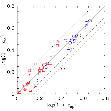
Figure 9: Photometric vs spectroscopic redshifts. Solid line is the $z_{ph}=z_{sp}$ relationship, dotted lines mark the 20% “error” in $1+z_{ph}$ and dashed lines mark the 30% “error” in $1+z_{ph}$. Hexagons are type 1 AGN, empty squares are type 2 AGN and asterisks are SGFs, as characterized by their SEDs discussed in subsection 5.1.

A number of spectroscopic redshifts are available to assess the quality of our photometric redshift determination. For 22 objects redshifts were obtained in the context of the XMM - LSS follow up programs and made available to us (Garcet et al., in prep.). Redshifts for two sources were taken from Lacy et al. (2006), who present optical spectroscopy of luminous AGN selected in the mid-IR from Spitzer observations. For XMDS 842 a redshift is available from NED.

The VVDS spectroscopic sample (see Gavignaud et al. 2006 for type 1 AGN) yields redshifts for 8 sources in the present sample. To obtain a larger redshift comparison set, we added 16 additional sources from the larger X-ray sample discussed in Paper I having a redshift from the VVDS spectroscopic survey. For the latter similar photometric data are available so that photometric redshifts could be estimated with the same procedure described above. In total, the spectroscopic comparison sample consists of 49 sources. For 3 of them, falling outside the area covered by SWIRE, only optical data were available for the SED.

Photometric and spectroscopic redshifts are compared in Fig. 9. The reliability and accuracy of the photometric redshifts are usually measured via the fractional error $\Delta z=\left(\frac{z_{phot}-z_{spec}}{1+z_{spec}}\right)$ and the rate of catastrophic outliers, defined as the fraction of sources with $|\Delta z|>$ 0.2. For our 49 objects, the mean $\Delta z$ is consistent with 0.00, with a 1 $\sigma$ dispersion of 0.12, and the outlier fraction is 10%. These results are significantly better than previously obtained for AGN samples, where the fraction of outliers is usually higher than 25% (Kitsionas et al., 2005; Babbedge et al., 2004). The achieved accuracy still does not allow us to consider photometric redshifts as fully reliable for individual sources, however it is adequate for a statistical analysis of the population. For a more detailed discussion, see Polletta et al. (2007).

The distribution of the 124 photometric redshifts (including the optically blank fields, for which only IR fluxes were used) is shown in Fig. 10. The majority (60%) of sources has $z<1$, with a tail extending up to $z\sim 4$. These results are consistent with the redshift distribution of other X-ray selected samples with similar or deeper flux limit (e.g. Barger et al., 2003; Hasinger, 2003; Barger et al., 2005).

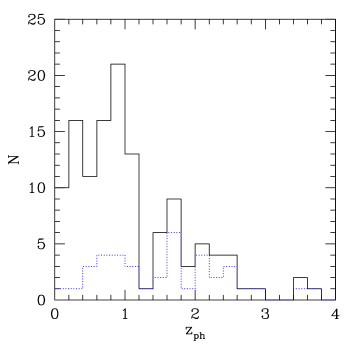
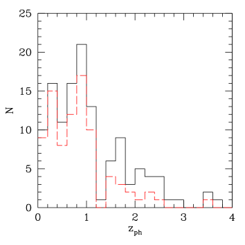
Figure 10: The distribution of photometric redshifts is shown as solid histogram in both panels. The dotted and dashed histograms (left and right panels, respectively) refer to the subsamples of unobscured and obscured AGN, respectively, discussed in subsection 5.1.

5.1 Spectral energy distributions and classification

According to the template which gives the best-fit solution, we assigned sources to one of the following broad classes: type 1 AGN, type 2 AGN, or SFG. The type 1 AGN class corresponds to sources best-fitted with a QSO1 template. The type 2 AGN class includes sources best-fitted with either the Seyfert 2 templates, or the composite AGN + starburst templates, or the QSO2 template. The SFG class includes sources fitted by a spiral or a starburst template. Elliptical templates never yielded best fit solutions.

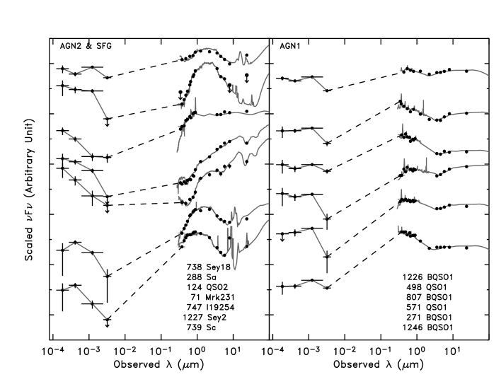
Figure 11: Observed SED (filled circles) and redshifted best-fit templates (grey solid curves) of 13 sources: 2 with star-forming like SEDs (left panel), 5 with type 2 AGN SEDs (left panel), and 6 with type 1 AGN SEDs (right panel). Downward pointing arrows correspond to 5$\sigma$ upper limits. The source sequence number and best-fit template names are listed in the same order as the SEDs are plotted.

Examples of observed SEDs with their best fit templates are presented in Fig. 11. For sources with both optical, near and mid-IR data, the photometric classification should be reliable since the SED shape of the different classes has specific signatures that can be easily identified. Interestingly, while photometric redshifts for type 1 AGN might be the most uncertain, their classification is instead rather easy. Note however that the Seyfert 1.8 template appears intermediate between type 1 and type 2 AGN (see Fig. 11). There is a large variety of SED shapes among the templates used for type 2 AGN, composite and star forming galaxies. In case the fit is not optimal or when only few IR data points are available, the separation between the various classes is uncertain as can be guessed comparing the SEDs in the left panel in Fig. 11.

The SED fitting procedure yields 39 type 1 AGN (32%), 61 type 2 AGN (49%) and 24 SFG (19%).

Comparing the SED classification with the spectroscopic one, we find that all the 16 objects classified as type 1 AGN from the fitted template indeed show broad emission lines in their optical spectra. Thus a photometric type 1 AGN classification appears unambiguous.

On the other hand, there are 10 objects spectroscopically classified as type 1 AGN, which are instead not recognized as such by the SED fitting procedure, indicating that our method systematically underestimates the fraction of broad line AGN. Specifically of the 10 misclassified objects 8 are fitted by a Seyfert 1.8 template (all with A_V close to 0), one by a QSO 2 template and 1 by a SFG template. These objects appear to be dominated by star-light emission in the optical and near-IR where the AGN continuum does not emerge clearly, although broad emission lines are visible in the optical spectrum. Of the remaining 23 objects without broad lines in their optical spectra only 5 are fitted with a Seyfert 1.8 template, in three cases with significant extinction. We conclude that SEDs fitted by Seyfert type 1.8 templates are intermediate between type 1 and type 2 objects and that our method systematically underestimates the objects spectroscopically classified as type 1.

The sources photometrically classified as SFGs do not show any AGN signature at optical and IR wavelengths, however the X-ray to optical and X-ray to IR ratios and the X-ray luminosity unambiguously point to the presence of AGN activity also in these objects.

In the following we will define optically “unobscured” AGN all sources fitted by a type 1 AGN template. These sources are expected to unambiguously correspond to broad line AGN. We will define all other sources (i.e. having either type 2 AGN or SFG like SEDs) as optically “obscured” AGN. As shown above, the latter group may include some AGN with broad emission lines, but with a SED dominated by the host galaxy in the near-IR. We will take into account where relevant that the number of unobscured objects should be corrected upwards by a factor 1.6 (and the number of obscured objects reduced accordingly).

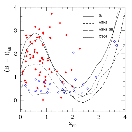
Figure 12: $B-I$ distribution of sources in the 3 $\sigma$ sample as a function of photometric redshift. Empty diamonds are unobscured AGN, filled diamonds are obscured AGN. Overimposed to points are the evolutionary tracks for an Sc galaxy (solid line), for a type 1 QSO (dotted line), for a type 2 AGN (short-dashed line) and a type 2 AGN plus a starburst component (long-dashed line).

In Fig. 12, we compare the classification based on the SED shape with the optical color $B-I$ as a function of redshift. The horizontal dashed line corresponds to the threshold between blue and red sources ($B-I=1$). 90% of the unobscured AGN have blue optical color and 84% of obscured AGN are red. Thus the simple classification based on observed color appears in retrospect rather successful when compared with the more sophisticated template fitting procedure. However, while at $z<1.6$ the SED and “color” classifications practically coincide (except for 2 obscured objects near the borderline), at larger redshifts there is a degeneracy among the different evolutionary tracks so that the optical color alone is not indicative of a spectral type.

Based on the photometric classification, the redshift distributions of unobscured and obscured AGN can be derived. They are shown in the left and right panels of Fig. 10, respectively. The two are clearly different, the first being broader and reaching higher redshifts, while the second is more concentrated at $z<1$ (72%). Several authors (e.g. Eckart et al., 2006; Steffen et al., 2004; Treister et al., 2005; La Franca et al., 2005) find different redshift distributions for type 1 and non type 1 AGN. An analysis of the fraction of unobscured and obscured AGN as a function of redshift will be discussed in Section 8.

6 X-ray spectral properties

We studied the X-ray spectral properties of our sample performing spectral fitting for individual sources with a sufficient number of counts (subsection 6.1) and a hardness ratio analysis for for faint sources to obtain individual values of N_H (subsection 6.2). A stacking technique was then used to study systematic trends in the whole sample (subsection 6.3). The general hardness ratio definition is

$$\mbox{HR}=\frac{CR_{H}-CR_{S}}{CR_{H}+CR_{S}}$$ (1)

where $CR_{H}$ and $CR_{S}$ are the count rates in the hard and in the soft band, respectively. In subsection 6.2 we consider three hardness ratio values for each sources, HR_CB, calculated using the energy bands $0.5-2$ (B) and $2-4.5$ keV (C), HR_DC, using the energy bands $2-4.5$ and $4.5-10$ keV (D) and HR, computed between the energy bands $0.5-2$ and $2-10$ keV.

6.1 Individual sources

We extracted X-ray spectra for all sources in the 3 $\sigma$ hard sample having at least 50 net counts in the MOS + pn merged image in the $2-10$ keV band. There are 55 X-ray sources in our catalogue which satisfy this criterion; 24 of them are optically unobscured AGN, and 31 are optically obscured AGN.

Counts were extracted for each source using the XMM - Newton Science Analysis System (SAS) evselect task in a circular region with a radius of 20″, corresponding, for a point-like source, to an encircled energy fraction of $\sim 70-75$% (off-axis angles between 0 and 10′). The pn data were used, unless the source was close to a CCD gap, in which case we used the MOS data, fitting simultaneously MOS1 and MOS2. Background counts were extracted from the nearest source free region, excluding areas near gaps in the CCD array. We used the SAS rmfgen task to create response matrices (one for each camera and each XMDS pointing) and arfgen to generate ancillary response files (one for each source).

X-ray spectra were analyzed using the XSPEC package (v. 11.3.1). We considered the energy range $0.3-10$ keV. When the number of counts was large enough, data were binned in order to have at least 15 or 20 counts for each energy channel and $\chi^{2}$ statistics was used, otherwise we used Cash statistics (Cash, 1979), which, however, does not give a “goodness of fit” evaluation, like the $\chi^{2}$. In order to better match the spectral resolution of the instruments, we binned the data of these sources with few counts using a fixed number of PHA channels before fitting using the Cash statistics.

We first fitted the spectra using a simple power law model with galactic absorption computed at the XMDS position (N${}_{H}=2.6\times 10^{20}$ cm^-2, Dickey & Lockman, 1990), plus a component for intrinsic absorption at $z=0$ (XSPEC model: phabs*zphabs*pow with abundance table of Wilms et al., 2000).

For all spectra for which $\chi^{2}$ statistics can be used in the fit (22 sources), we set both intrinsic column density and photon index as free parameters. Spectral fit results are reported in Table 5 in Appendix B. The errors in Tables and Figures correspond to the 90% confidence level for one interesting parameter. The average photon index is $\Gamma\sim 2.1$ and N${}_{H}<21$ cm ^-2. This is consistent with their location in the hardness ratio plot, where they cluster around HR${}_{CB}=-0.5$ and HR${}_{DC}=-0.5$ (see Table 5 and subsection 6.2). Therefore they cannot be considered representative of the whole sample.

Since more than half of the X-ray spectra in the sample do not have a sufficient number of counts to perform a fit with both $\Gamma$ and N_H free parameters, we fixed the photon index for all objects, in order to obtain an estimate of the column density. We used two different values of the photon index, $\Gamma=2.0$ and $\Gamma=1.7$, both appropriate for AGN (Turner & Pounds, 1989; Nandra & Pounds, 1994). Spectral fit results for the simple absorbed power law model for each source with both $\Gamma=2.0$ and $\Gamma=1.7$ are reported in Table 6 in Appendix B, where we also list the sources with peculiar fits. The best fit values of N_H obtained with $\Gamma=2.0$ are higher than those obtained with photon index frozen to 1.7, by about $\Delta\mbox{log(N}_{H})=0.2$. The two column density estimates are consistent within errors in 90% of cases.

We will consider in the following only the distribution obtained fixing $\Gamma=2.0$, except for two sources (XMDS 124 and 779): in these two cases we were able to find a stable solution only fixing the photon index to $\Gamma=1.7$. The column density distributions of optically obscured and unobscured AGN turn out to be different: 16% of unobscured AGN (3 out of 19) have N${}_{H}>10^{21}$ cm^-2, while more than 55% of obscured AGN (19 out of 34) have N${}_{H}>10^{21}$ cm^-2. We recall that these are lower limits to the column density values, since we did not yet introduce the redshift dependence.

Finally, we introduced the photometric or spectroscopic redshift, when available, in order to compute the intrinsic column density. The photon index was left free when the $\chi^{2}$ statistics could be used, otherwise it was fixed to 2.0. Spectral fit results, along with redshifts, are reported in Table 6 in Appendix B. Again, the distributions for optically obscured and unobscured AGN are different, with 63% of obscured AGN (19 out of 30) having N${}_{H}>10^{21}$ cm^-2 and 36% (11 out of 30) with N${}_{H}>10^{22}$ cm^-2. For comparison, only $\sim 20$% of unobscured AGN (4 out of 21) have N${}_{H}>10^{21}$ cm^-2 and 10% (2 out of 21) have N${}_{H}>10^{22}$ cm^-2.

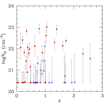
Figure 13: Intrinsic column density vs photometric or spectroscopic redshift. Empty diamonds are optically unobscured AGN, filled diamonds are optically obscured AGN.

In Fig. 13 the intrinsic column density is shown as a function of redshift; this figure is qualitatively consistent with those presented in other surveys (e.g. Eckart et al., 2006) and shows no obvious trend with $z$, although we also notice the paucity of high redshift sources with well constrained measures of N_H.

6.2 X-ray absorption

The two hardness ratios HR_CB and HR_DC defined above are compared in Fig. 14. As expected, most sources lie along the values expected for a single power law model. We further distinguish obscured/unobscured sources with different symbols. Less than 10% of the objects classified as optically unobscured AGN have HR${}_{CB}>-0.3$ (N${}_{H}\sim 10^{21.5}$ at $z=0$), while more than 40% of the sources classified as obscured AGN have HR${}_{CB}>-0.3$ indicating that X-ray absorption and an obscured classification are often associated.

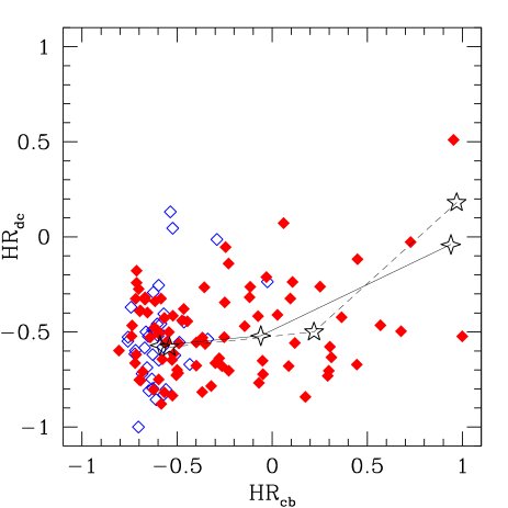
Figure 14: X-ray color - color plot for sources in the 3 $\sigma$ hard sample. Energy bands involved are: $0.5-2$ $(B)$, $2-4.5$ $(C)$ and $4.5-10$ keV $(D)$. Sources are classified as optically unobscured AGN (empty diamonds) or obscured AGN (filled diamonds). We also mark the hardness ratios computed for a simple absorbed power law spectral model, with $\Gamma=2$ and logN_H = 21, 22, 23 for $z=0$ (four point stars connected by the solid line, from left to right) and logN_H = 22, 23, 24 for $z=1$ (five points stars connected by the dashed line, from left to right).

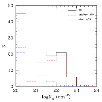
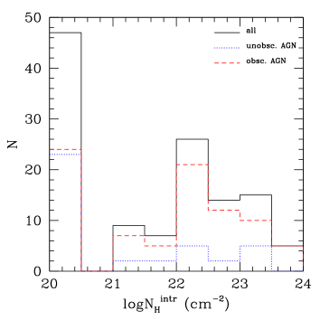
Figure 15: Distribution of observed (left panel) and intrinsic (right panel) column densities. Solid histogram refers to the whole sample, dotted and dashed histograms refer to optically unobscured AGN and optically obscured AGN, respectively.

For a quantitative estimate of the absorbing column N_H we used the results of the spectral fits described in Section 6.1 with $\Gamma$ fixed to 2.0 for the 51 brightest sources and computed the column density from the X-ray hardness ratios in the remaining cases in the following way.

We used the standard hardness ratio HR, computed between the $2-10$ and the $0.5-2$ keV bands. We made simulations using XSPEC to obtain hardness ratios corresponding to typical values of N_H ranging from $10^{20}$ to $10^{24}$ cm^-2. A simple power law model with photon index $\Gamma=2.0$ was assumed, consistently with the model used for the X-ray spectral analysis. The simulations and the objects for which a spectrum could be extracted define a clear relationship between N_H and HR for HR $>-0.5$, while, below these values, the HR - N_H relation degenerates. We therefore fixed the latter value, corresponding to N${}_{H}\sim 10^{21}$ cm^-2, as a threshold below which all column densities are fixed to the galactic value. By interpolation we computed the observed N_H corresponding to the hardness ratio of each source. The intrinsic column density was then obtained from the observed one using the photometric (or spectroscopic, when available) redshift and the expression N${}_{H}^{intr}=\mbox{N}_{H}^{obs}(1+z)^{2.6}$ (Barger et al., 2002), also when the observed column density was estimated from the spectrum (i.e. in this cases we did not use the N${}_{H}^{intr}$ obtained by the XSPEC and reported in Table 6, but we recomputed it from the observed value, in order to be more consistent with the column density estimates obtained from HR). N${}_{H}^{intr}$ was not computed when the observed column density was fixed at the galactic value.

The observed and intrinsic column density distributions are reported in Fig. 15. Different lines (dotted/dashed) refer to the N_H distribution for optically unobscured and obscured AGN respectively. Unfortunately, our choice of setting a fixed value for low N_H creates an artificial gap in the distribution. The majority of optically obscured AGN are X-ray absorbed (N${}_{H}^{intr}>10^{22}$ cm^-2), as expected. We find that also 12 unobscured AGN (more than 30%) have N${}_{H}^{intr}>10^{22}$ cm^-2. It is well known that N_H values are less well constrained with increasing redshifts (see e.g. Eckart et al., 2006; Akylas et al., 2006; Tozzi et al., 2006), since the absorption cut - off shifts to lower energies and becomes comparable to the galactic values or even drops out of the observed band. For $z\ga 1.5$, an intrinsic N_H of $10^{22}$ cm^-2 corresponds to an observed column density $\la 10^{21}$ cm^-2. Unobscured AGN, whose hardness ratios generally cluster around $-0.5$ (which corresponds to N${}_{H}^{obs}\sim 10^{21}$ cm^-2), are more severely affected by this problem than obscured AGN, which have a broader HR distribution. We have partially compensated for this effect with our choice of fixing intrinsic columns to 0 when the observed hardness ratio HR $\sim-0.5$. Moreover, we have at least 4 examples of optically unobscured AGN (XMDS 12, 258, 280 and 406) in which the $observed$ N_H is already larger than N${}_{H}=5\times 10^{21}$ cm^-2, ensuring that the large columns are not all to be attributed to the redshift effects.

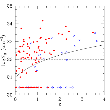
Figure 16: Intrinsic column density vs photometric (or spectroscopic, when available) redshift. Empty diamonds are optically unobscured AGN and filled diamonds are optically obscured AGN. The dashed line marks the threshold between X-ray absorbed (N${}_{H}>10^{22}$ cm^-2) and unabsorbed sources. The solid line shows the intrinsic column density that would be derived at a given redshift, for a measured column density of $10^{21}$ cm^-2 in the observer frame.

On the other hand, among the objects for which we are not able to estimate the column density (those with N_H fixed at the galactic value), there could be some which could be really X-ray absorbed. In Fig. 16 we show the intrinsic column density of our objects as a function of redshift. The solid line shows the intrinsic N_H values that would be derived at a given redshift, for an observed column density of $10^{21}$ cm^-2. Since the objects with HR $<-0.5$ should have N${}_{H}^{obs}<10^{21}$ cm^-2, their intrinsic column density should lie below the solid line in Figure. It is therefore possible that we underestimate the number of X-ray absorbed objects for redshift $z\ga 1.5$ (where the solid and dashed line cross). The column densities are therefore difficult to estimate at high redshift, but this should not affect our results.

6.3 Stacking analysis

Given that less than half of the sources in our sample have a sufficient number of counts to perform a spectral analysis, we used a stacking technique to measure the spectral properties, averaged over the whole redshift range, of sources of different classification and in different flux intervals.

For the stacking analysis we used only pn data, because of the pn larger effective area; we selected only sources which are not in or near a pn CCD gap or bad column. Moreover, since the pn point spread function (PSF) and the vignetting are not well determined for large off-axis angles (Ghizzardi, 2002; Kirsh, 2006) we only used sources with off-axis angle $\theta<11^{\prime}$. This value allows us to obtain a significant number of sources (83), for which calibration should be still reliable. 30 sources are optically unobscured AGN and 53 are optically obscured AGN.

We restricted the source area to a fixed radius of 15″, which, on-axis, corresponds to 67% of the encircled energy for a point-like source. Since with this radius we sample the PSF core and not the wings, the encircled energy fraction has a weak dependence on the off-axis angle (at $\theta=10^{\prime}$ 67% of the encircled energy is within a 16″ radius) and the energy dependence can also be neglected. Therefore, we can consider all sources together regardless of their position in the field. A background spectrum was extracted for each source in a circle of radius 80″ in the nearest source free region. Ancillary response files were also produced for each source, while, as for single spectra analysis, we used one response matrix for each XMM - Newton pointing.

The sample used in the stacking analysis covers a flux range from about $10^{-14}$ to $1.2\times 10^{-13}$ erg cm^-2 s^-1; we divided it in 5 flux bins, chosen to have a sufficient number of counts in each bin (see Table 1; on average, brighter sources have a greater number of counts, so in the higher flux bins a smaller number of sources is included).

The spectra within the same flux bin were added using the mathpha task of ftools to produce a single spectral file. The same was done for background files. The auxiliary and response files were combined using the addarf and addrmf tasks of ftools, respectively. The combined spectra were grouped to a minimum of 20 counts per bin and were analyzed using XSPEC.

Flux bins	N. of sources	$\Gamma$
$-14.1<\mbox{log}F_{X}<-13.7$	25	$1.72^{+0.09}_{-0.09}$
$-13.7<\mbox{log}F_{X}<-13.6$	22	$1.81^{+0.09}_{-0.08}$
$-13.6<\mbox{log}F_{X}<-13.5$	15	$1.83^{+0.10}_{-0.09}$
$-13.5<\mbox{log}F_{X}<-13.3$	14	$1.76^{+0.08}_{-0.08}$
$-13.3<\mbox{log}F_{X}<-12.9$	7	$1.75^{+0.12}_{-0.12}$

Table 1: Mean spectral properties from the stacking analysis of sources in the $3\sigma$ hard sample detected in the pn at off-axis angle $<11$′. N_H is fixed to the galactic value.

Optically unobscured AGN			Optically obscured AGN
Flux bins	N. of sources	$\Gamma$	Flux bins	N. of sources	$\Gamma$
$-14.1<\mbox{log}F_{X}<-13.6$	12	$1.91^{+0.12}_{-0.12}$	$-14.1<\mbox{log}F_{X}<-13.7$	16	$1.60^{+0.10}_{-0.09}$
$-13.6<\mbox{log}F_{X}<-13.5$	8	$2.04^{+0.09}_{-0.09}$	$-13.7<\mbox{log}F_{X}<-13.6$	19	$1.75^{+0.07}_{-0.07}$
$-13.5<\mbox{log}F_{X}<-13.3$	7	$1.85^{+0.11}_{-0.10}$	$-13.6<\mbox{log}F_{X}<-13.4$	12	$1.57^{+0.09}_{-0.08}$
$-13.3<\mbox{log}F_{X}<-12.9$	3	$2.13^{+0.21}_{-0.20}$	$-13.4<\mbox{log}F_{X}<-12.9$	6	$1.49^{+0.10}_{-0.09}$
			SFGs
			$-14.1<\mbox{log}F_{X}<-13.6$	7	$1.33^{+0.17}_{-0.16}$
			$-13.6<\mbox{log}F_{X}<-12.9$	6	$1.21^{+0.11}_{-0.10}$

Table 2: Mean spectral properties from the stacking analysis of optically unobscured, optically obscured AGN and of the subclass of SFG objects. N_H is fixed to the galactic value.

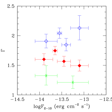
Figure 17: Photon index obtained from the fit of stacked spectra as a function of X-ray flux for the optically unobscured AGN (empty diamonds), optically obscured AGN (filled diamonds) and SFGs (crosses). Vertical bars are errors on $\Gamma$, while horizontal bars show the flux bin width.

We fitted the stacked spectra in the $0.3-10$ keV range using a single power law model with column density fixed to the galactic value. The fit results are reported in Table 1. The $\Gamma$ values obtained for the whole sample are consistent within errors with $\Gamma=1.7-1.8$ in all the flux bins.

We then considered the optically unobscured and obscured AGN separately. We divided them in 4 bins, using two slightly different binnings for the two subsamples dictated by the available statistics. The results are reported in Table 2 and the photon index as a function of flux is shown in Fig. 17. The difference between the optically unobscured and obscured AGN populations is evident: for the unobscured AGN the measured photon index is consistent with $\Gamma=2$ over the whole flux range, while for the optically obscured it is consistent with $\Gamma=1.5-1.6$. Therefore the observed average spectral slope of unobscured AGN is consistent with that of typical broad line AGN (Turner & Pounds, 1989; Nandra & Pounds, 1994), while that of optically obscured AGN is significantly harder. No significant dependence of the spectral index with flux is found for optically unobscured or optically obscured AGN.

Georgakakis et al. (2006) merged the X-ray spectra of hard X-ray sources detected by XMM - Newton at $F_{2-8}>2\times 10^{-14}$ erg cm^-2 s^-1 and having an optical counterpart in the Sloan Digital Sky Survey (York et al., 2000) with red color ($g-r>0.4$). They found that the stacked spectrum of these sources has a spectral slope of $\Gamma=1.47\pm 0.04$ (sources observed with the THIN filter), consistent with that of the XRB ($\Gamma\sim 1.4$, Gendreau et al., 1995; Chen et al., 1997; Vecchi et al., 1999). As shown in the previous Sections, optically obscured AGN generally have red optical color and the average spectral slope obtained for obscured AGN is only slightly higher than that of red objects of Georgakakis et al. (2006), showing that we are sampling similar populations.

According to Worsley et al. (2005), whilst the XRB is $\sim 85$% and $\sim 80$% resolved in the $0.5-2$ and $2-10$ keV bands respectively, it is only $\sim 60$% resolved above $\sim 6$ keV and $\sim 50$% resolved above $\sim 8$ keV. The missing population should be made of faint, heavily obscured AGN located at redshift of $\sim 0.5-1.5$, and with intrinsic absorption of $\sim 10^{23}-10^{24}$ cm^-2. As noted in Section 5, the sources classified as SFG do not show any AGN signature in the optical and IR. We also find that the fraction of X-ray absorbed sources in the SFG class ($\sim 67$%, 16 out of 24) is larger than that of X-ray absorbed sources in the type 2 AGN class ($\sim 54$%, 33 out of 61). Thus sources belonging to this class appear to be good candidates to be responsible for the XRB in the harder X-ray range. We therefore applied the stacking analysis to study separately the spectral properties of the SFG population in our sample.

Only 13 SFGs are detected in the pn at off-axis angle $<11$′, so we grouped them in two flux bins. The spectral fits of the SFG stacked spectra give $\Gamma\sim 1.2-1.3$, with no significant differences in the two bins (Table 2 and crosses in Fig. 17). Therefore the average spectra of the SFGs are harder than those of optically obscured AGN (type 2 + SFGs) and even harder than the XRB spectrum in the same band. If the population responsible for the high energy XRB has the same SED properties as the SFG objects discussed in this work, they might go unidentified as AGN even in the IR, where they look like star forming galaxies. A more detailed discussion about this topic is presented in Polletta et al. (2007).

7 The surface density of optically obscured and unobscured AGN

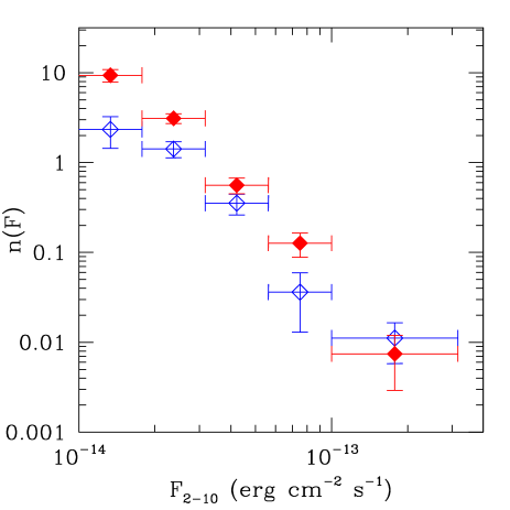
Figure 18: Differential logN-logS for unobscured (empty diamonds) and obscured AGN (filled diamonds). The units of $n(F)$ are number per 10^-15 erg cm^-2 s^-1 deg^-2. Vertical bars show the error on the number of sources, while the horizontal bars show the flux bin width.

In Paper I we computed the logN-logS distribution for all the sources detected with a probability of false detection $P<2\times 10^{-5}$ in the $0.5-2$ and $2-10$ keV bands; for the $2-10$ keV band, this probability threshold is slightly lower than the 3 $\sigma$ threshold chosen for the present sample, therefore all the sources of the 3 $\sigma$ hard sample were included in the logN-logS. We used the differential logN-logS for the $2-10$ keV band reported in Paper I, computed the fraction of optically unobscured and obscured AGN in each flux bin from the present sample and rescaled the logN-logS relationship accordingly. We made the reasonable assumption that the fraction of optically obscured and unobscured AGN should be the same in the area covered by the VVDS as well as in the whole XMDS area.

The differential logN-logS relationships for optically obscured and unobscured AGN are shown in Fig. 18. The errors are the combination of the errors on the original logN-logS with those on the fractions, according to the error propagation formula. The two logN-logS are quite similar, except for the faintest fluxes, where the density of the optically unobscured AGN is significantly lower (by a factor of $\sim 4.6$) than that of optically obscured AGN. Considering the cumulative logN-logS instead of the differential one, we can give an estimate of the integral surface density of optically obscured and unobscured AGN at $F>10^{-14}$ erg cm^-2 s^-1. We find 138 and 59 sources deg^-2, respectively, and the ratio between optically obscured and unobscured AGN is $\sim 2.3$ for the whole flux range covered. The ratio would decrease from 2.3 to 1.1 if we assume that the fraction of unobscured AGN should be corrected by a factor of 1.6 (see subsection 5.1).

We compared these values with the surface densities of broad line and non broad line AGN, estimated by Bauer et al. (2004) in their study of the Chandra Deep Fields. We obtained values from their Fig. 4 and 8. At $F_{2-10}>10^{-14}$ erg cm^-2 s^-1, the surface densities differ by a factor of $\sim 2$. This discrepancy is a consequence of the fact that the logN-logS computed in Paper I is lower than that of Bauer et al. (2004). As discussed in Paper I, the XMDS logN-logS is slightly lower than those of Baldi et al. (2002) and Moretti et al. (2003) for $F_{2-10}>2\times 10^{-14}$ erg cm^-2 s^-1, but consistent within the errors. Instead, the Bauer et al. (2004) surface density for fluxes $F_{2-8}\sim 10^{-14}$ erg cm^-2 s^-1 is slightly higher than that obtained by Moretti et al. (2003). Since all these surveys refer to small connected areas in different parts of the sky, it is possible that the differences in the derived number counts may be due to cosmic variance.

On the other hand, the Bauer et al. (2004) ratio of non broad line and broad line AGN at $F\sim 10^{-14}$ is $\sim 1.5-2$, intermediate between our values of 2.3 and 1.1. These authors describe some caveats about their AGN classification criteria, and point out that their number counts of broad line AGN must be considered a lower limit and that of non broad line AGN an upper limit, so that their non broad line/broad line AGN ratio could approach our lower estimate.

7.1 Type 2 QSO candidates

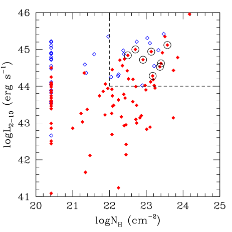
Figure 19: X-ray ($2-10$ keV) absorption corrected luminosity vs intrinsic column density. Empty diamonds are optically unobscured AGN and filled diamonds are optically obscured AGN. Encircled points are objects with $F_{X}/F_{R}>40$. The dashed lines mark the region where type 2 QSOs should be found.

We searched for type 2 QSO candidates in the 3 $\sigma$ hard sample. In the X-ray domain the type 2 QSO population is characterized by high intrinsic absorption (N${}_{H}>10^{22}$ cm^-2) and high X-ray luminosity ($L_{X}>10^{44}$ erg s^-1). Since locally (in the Seyfert luminosity regime) X-ray absorbed AGN are 4 times more numerous than unabsorbed ones (Maiolino & Rieke, 1995; Risaliti et al., 1999), according to the unified AGN model, one would expect that the same should be true at high luminosities and redshifts, i.e. in the QSO regime. A still undiscovered large population of obscured AGN is indeed predicted by X-ray background synthesis models (e.g. Gilli et al., 2001; Franceschini et al., 2002; Gandhi & Fabian, 2003; Ueda et al., 2003; Worsley et al., 2005). Before the advent of Chandra and XMM - Newton, only a few type 2 QSOs were known (see e.g. Akiyama et al., 1998; Della Ceca et al., 2000; Franceschini et al., 2000). Deep X-ray surveys found indeed a large fraction of the objects to be obscured (e.g. Barger et al., 2003; Mainieri et al., 2002), but the number of identified type 2 QSOs is still very low compared to the model predictions. A significant fraction of high - $z$, obscured QSOs may have escaped optical spectroscopic identification due to the weakness of their optical counterparts and misclassification due to the lack of AGN signature. On the other hand, medium deep X-ray surveys, covering relatively large sky areas at a higher flux limit, proved to be effective to select significant samples of type 2 QSO candidates among objects with high values of the X-ray to optical ratio ($F_{X}/F_{R}>10$, see Fiore et al., 2003). Recent findings also suggest a connection between Extremely Red Objects (EROs, $R-K>5$ in the Vega system) and type 2 QSOs (see e.g. Brusa et al., 2005; Severgnini et al., 2005, and references therein). Maiolino et al. (2006) suggest that by selecting extreme values of $F_{X}/F_{R}(>40)$ and extreme values of $R-K(>6)$, the type 2 QSO selection efficiency may approach 100%.

The absorption corrected X-ray luminosity is shown as a function of the intrinsic column density in Fig. 19. There is a significant number of objects (34 out of 124) having $L_{X}>10^{44}$ erg s^-1 and N${}_{H}>10^{22}$ cm^-2 in our sample. 12 of them (35%) are classified as unobscured AGN, while the remaining 22 are classified as obscured AGN, based on the SED classification. We verified that these objects generally have high X-ray to optical ratios, in particular 21 of the 25 X-ray sources in the 3 $\sigma$ sample having $F_{X}/F_{R}>10$ have N${}_{H}>10^{22}$ cm^-2 and $L_{2-10}>10^{44}$ erg s^-1. On the other hand, while for the optically unobscured AGN the fraction of high luminosity, X-ray absorbed sources having $F_{X}/F_{R}>10$ is only 25% (3 out of 12), this fraction is 77% (17 out of 22) for the obscured ones.

All the 8 objects with $F_{X}/F_{R}>40$ (the threshold used by Maiolino et al., 2006) satisfy the X-ray definition of a type 2 QSO (see encircled objects in Fig. 19). All are optically obscured. These results confirm that type 2 QSO candidates are found between the high X-ray to optical ratio population and that the threshold proposed by Maiolino et al. (2006) is highly efficient in finding type 2 QSOs but it is far from exhaustive (i.e. many type 2 QSOs have $F_{X}/F_{R}<40$).

Figure 20: Optical-infrared color (in the AB system) as a function of redshift for the type 2 QSO candidates compared with the expected colors for various types of galaxy and AGN templates. Filled circles are sources fitted by a type 1 AGN template, squares are sources fitted by a type 2 AGN template, asterisks are object fitted by a SFG template. Encircled points are objects having $F_{X}/F_{R}>40$. Triangle is SWIRE_J104409.95+585224.8 in Polletta et al. (2006), diamond is XBS J0216-0435 in Severgnini et al. (2006).

In Fig. 20 the color between VVDS $R$ band and SWIRE 4.5 $\mu$m band is shown as a function of redshift for the type 2 QSO candidates. Objects fitted by a type 1 AGN template have generally blue colors. About 70% of the candidates fitted by a type 2 AGN or a SFG template have extremely red infrared/optical flux ratios, as observed in extremely obscured AGN and similar to those observed in spectroscopically confirmed type 2 QSOs at high redshift ($z=1.5-2.5$, see Severgnini et al., 2006; Polletta et al., 2006). We have $K$ magnitudes from the UKIDSS Early Data Release or from the VVDS for 18 objects: 4 of them are EROs, all having $F_{X}/F_{R}>40$ and all fitted by a type 2 AGN or a SFG template. Given the blue optical/IR colors of the optically unobscured AGN, we exclude them from the type 2 QSO candidates. Therefore the sample of type 2 QSOs reduces to 22 objects. One of them (XMDS 55) has been indeed spectroscopically confirmed as a type 2 object (see Garcet et al. in prep.). The type 2 QSO candidates represent ($18\pm 4$)% of the sources in the 3 $\sigma$ hard sample and have X-ray fluxes in the range $1-5\times 10^{-14}$ erg cm^-2 s^-1.

As done before for optically obscured and unobscured AGN, we rescaled the surface density of X-ray sources at $F_{2-10}>10^{-14}$ erg cm^-2 s^-1 to the type 2 QSO fraction to estimate the type 2 QSOs surface density. It results ($35\pm 8$) deg^-2, lower but consistent, within errors, with ($45\pm 15$) deg^-2 found by Cocchia et al. (2007) in the HELLAS2XMM at the same flux level.

The type 2 QSO population represents about 35% of all high luminosity sources ($L_{X}>10^{44}$ erg s^-1) in our sample. For comparison, according to Perola et al. (2004), in the HELLAS2XMM the fraction of X-ray absorbed sources (N${}_{H}>10^{22}$ cm^-2) in the high luminosity ($L_{X}>10^{44}$ erg s^-1) AGN population would be between 28% and 40%.

8 Discussion

8.1 Optical Obscuration vs X-ray Absorption

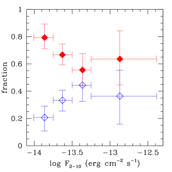
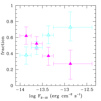
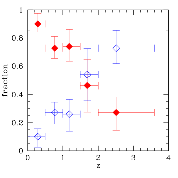
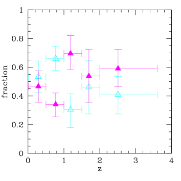
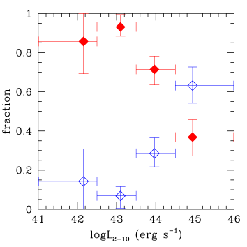
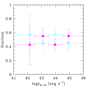
Figure 21: Left panels: fraction of optically obscured (filled diamonds) and unobscured (empty diamonds) AGN as a function of X-ray flux (upper panel), redshift (middle panel) and luminosity (lower panel). Right panels: fraction of X-ray absorbed (N${}_{H}>10^{22}$ cm^-2, filled triangles) and unabsorbed (empty triangles) AGN as a function of X-ray flux (upper panel), redshift (middle panel) and luminosity (lower panel).

The wide and well sampled multiwavelength coverage from the optical through the mid-IR allowed us to use the photometric approach to redshift determination and classification in a very effective way. The comparison with a spectroscopic sample gives us confidence in the estimated redshifts and in the fact that a photometric type 1 classification is unambiguous, but reveals a bias against the recognition of a number of broad line objects as type 1 SEDs. This is due to the coexistence of Seyfert 1.8 type SEDs with the presence of broad line emission. Since we adopt here the SED classification, these objects will be considered “optically obscured”. In optically obscured objects the optical-UV emission from the AGN may be either dimmed by intervening dust or be weaker than that of the host. In this sense, “red quasars” (Wilkes et al., 2002; Gregg et al., 2002; Glikman et al., 2004; Urrutia et al., 2005; Wilkes et al., 2005) would be classified here as obscured objects.

The X-ray data give us an independent and complementary information essential to identify AGN where the nuclear X-ray emission is heavily absorbed, and AGN features may be completely hidden both in the optical and IR bands, as in the case of sources identified with SFGs. In the following we discuss the trends of optical obscuration and X-ray absorption within our sample separately, in order to explore to what extent the two are associated.

Bins				N${}_{H}>10^{22}$
	Ntot	Opt. Unobsc.	Opt. Obsc.	Nabs	Opt. Unobsc.	Opt. Obsc.
$-14<\mbox{log}F_{2-10}<-13.75$	27	5	22	17	2	15
$-13.75<\mbox{log}F_{2-10}<-13.5$	61	20	41	32	8	24
$-13.5<\mbox{log}F_{2-10}<-13.25$	25	11	14	9	2	7
$-13.25<\mbox{log}F_{2-10}<-12.5$	9	3	6	2	0	2
$z<0.5$	28	2	26	13	0	13
$0.5<z<1$	42	11	31	14	1	13
$1<z<1.5$	21	5	16	15	3	12
$1.5<z<2$	11	6	5	6	1	5
$z>2$	20	15	5	12	7	5
log$L_{2-10}<42.5$	5	0	5	2	0	2
$42.5<\mbox{log}L_{2-10}<43.5$	27	1	26	15	0	15
$43.5<\mbox{log}L_{2-10}<44.5$	54	15	39	23	4	19
log$L_{2-10}>44.5$	36	23	13	20	8	12

Table 3: Total number of sources, number of optically unobscured and optically obscured AGN, number of X-ray absorbed AGN (N${}_{H}>10^{22}$ cm^-2), and number of optically unobscured and obscured AGN among X-ray absorbed AGN in each X-ray flux, redshift and absorption corrected X-ray luminosity bin (see text and Fig. 21). Fluxes are in erg cm^-2 s^-1, luminosities are in erg s^-1.

The sample contains 39 optically unobscured AGN and 83 optically obscured AGN (of which 22 best fitted by a SFG template). The two sources with X-ray to optical ratios and luminosities typical of normal galaxies are excluded from this analysis. The X-ray absorbed AGN are 60. X-ray absorption occurs in 48 of the 83 obscured AGN (of which 16 are SFGs). The remaining 12 X-ray absorbed AGN are classified as unobscured on the basis of their SEDs. We conclude that X-ray absorption is commonly but not exclusively associated with obscuration since 30% of the unobscured AGN are X-ray absorbed.

The numbers of optically unobscured, optically obscured and X-ray absorbed AGN in different flux, redshift and luminosity bins are given in Table 3, where we also report separately the number of X-ray absorbed sources within the optically unobscured and obscured AGN respectively.

The fractions of obscured/absorbed AGN in our sample are shown in Fig. 21 as a function of observed flux, redshift and absorption corrected hard X-ray luminosity. The left panels refer to optically obscured and unobscured AGN, while the right panels refer to X-ray absorbed (N${}_{H}^{intr}>10^{22}$ cm^-2) and unabsorbed AGN, irrespectively of their SED classification.

We used the Bayesian statistics to estimate the “true value” of the fractions and their errors (68% credible interval, see Andreon et al., 2006, and references therein) and to evaluate the reliability of the suggested correlations. We tested whether existing data support a model in which the fraction 1) is constant or 2) has a linear dependence with redshift, flux or luminosity, by computing the Bayesian Information Criterion (BIC, Schwartz 1978; an astronomical introduction to it can be found in Liddle 2004) for both models and then the difference $\Delta$BIC between the BICs of the two models. A $\Delta$BIC of 6 or more can be used to reject the model with the largest value of BIC, whereas a value between 2 and 6 is only suggestive (Jeffreys, 1961). We also compared the trends of optically obscured and X-ray absorbed AGN using the same criterion.

Obscured sources are dominant in the lowest flux bin ($79^{+0.10}_{-0.08}$%, upper left panel), although a systematic trend of optically obscured AGN to decrease with X-ray flux is not established ($\Delta$BIC = 0.7). This result was already apparent from the logN-logS curves, where the surface density of optically obscured AGN largely exceeds that of unobscured objects in the lowest flux interval ($F<2\times 10^{-14}$ erg cm^-2 s^-1), see Fig. 18. The fraction of X-ray absorbed AGN (upper right panel) is also higher at the faintest fluxes and there is a positive indication that it changes systematically with flux ($\Delta$BIC = 4.9).

The fraction of optically obscured AGN shows instead a steep decrease as a function of redshift (middle left panel), from $\sim 90$% at $z<0.5$ to $\sim 30$% at $z>2$, and the trend is highly significant ($\Delta$BIC = 26.3). Similarly, the data strongly support a decrease of the fraction of optically obscured AGN with luminosity (lower left panel, $\Delta$BIC = 23.9). The two trends are not independent, since in flux limited surveys a correlation between luminosity and redshift is expected. For X-ray absorbed AGN, data suggest constancy with both redshift and luminosity. In summary there is evidence that the trends of optically obscured and X-ray absorbed AGN are different both as a function of redshift ($\Delta$BIC = 17.5) and luminosity ($\Delta$BIC = 20.1), the former showing a decrease with redshift and luminosity, the latter being essentially constant.

8.2 Comparison with the literature

Several authors compute the fraction of X-ray absorbed or optically obscured AGN as a function of all or some of the quantities described above, however in the literature a detailed comparison between optical obscuration and X-ray absorption seems to be lacking.

The trends of broad line AGN as a function of redshift and X-ray luminosity are explored e.g by Steffen et al. (2003), Barger et al. (2005), Treister & Urry (2005), Tozzi et al. (2006), who use data from the Chandra Deep Fields, in some cases complemented by shallower Chandra observations. All these samples reach flux levels significantly deeper than ours thus probing the AGN population in more depth; given this, we limit ourselves to a qualitative comparison. Assuming that unobscured AGN correspond to broad line AGN, the trends presented by the above authors are in agreement with those shown in the middle and lower left panels of Fig. 21.

We examined in more detail the data of the HELLAS2XMM 1df (Fiore et al., 2003; Perola et al., 2004) and of the Serendipitous Extragalactic X-ray Source Identification (SEXSI, Eckart et al., 2006), whose flux limits and areas are comparable to those of the XMDS. For the HELLAS2XMM, we computed the fraction of optically obscured AGN using all the sources for which a spectroscopic classification is available (their samples S1, S2 and S4). Consistently with our classification scheme, we grouped together the objects spectroscopically classified as type 2 AGN, emission line galaxies (ELGs) and early type galaxies (ETGs), considering them as optically obscured AGN. We did the same for the SESXI data, considering as optically obscured AGN all sources spectroscopically classified as narrow line AGN (NLAGN), ELGs and absorption line galaxies (ALGs). Broad line AGN are instead classified as optically unobscured.

We computed the fractions in the HELLAS2XMM and SEXSI using the Bayesian statistics, as done for our sample. We find that also in the HELLAS2XMM and SEXSI cases the fraction of optically obscured AGN decreases (and conversely the fraction of optically unobscured AGN increases) with redshift and luminosity. We notice that in the HELLAS2XMM survey the fraction of unobscured AGN is larger by a factor of $\sim 3$ than ours, for redshifts $z<1.5$, while it is consistent with ours at higher redshifts. The agreement with the SEXSI survey is instead better. The spectroscopic completeness is however about 90% for the HELLAS2XMM, while it ranges from 40% to 70% for the SEXSI. The larger fractions of type 1 AGN in spectroscopic samples are expected, given the differences between photometric and spectroscopic classifications discussed above, however the fraction of type 1 AGN in the HELLAS2XMM is still larger than ours even when the correction factor computed in subsection 5.1 is taken into account. Nevertheless, the trends observed in spectroscopic samples are consistent with ours.

The X-ray properties (fraction of AGN with N${}_{H}>10^{22}$ cm^-2) are explored by a number of authors who use XMM - Newton or Chandra data of similar depth (flux limit of $\sim 10^{-14}$ erg cm^-2 s^-1, see e.g. Piconcelli et al., 2003; Perola et al., 2004; Eckart et al., 2006; Akylas et al., 2006) and a quantitative comparison with their results is possible. Taking into account the different selection criteria and corrections that the different authors apply to the data, we find agreement within the errors with the results reported here.

Again, we concentrated in particular on the results obtained in the HELLAS2XMM and in the SEXSI surveys. Both Perola et al. (2004) and Eckart et al. (2006) show that the fraction of X-ray absorbed AGN increases with decreasing X-ray flux, even if the trends are significant only when X-ray fluxes as faint as $10^{-15}$ erg cm^-2 s^-1 are considered. In our flux range, we are consistent with the HELLAS2XMM and SEXSI values. Perola et al. (2004) and Eckart et al. (2006) also find that there is no evidence of a dependence of the fraction of X-ray absorbed AGN on luminosity. Again, these results are consistent with ours, with a better quantitative agreement with the SEXSI than with the HELLAS2XMM survey (for example, the fraction of X-ray absorbed AGN is between $\sim 0.4$ and $\sim 0.6$ in our case and in the SEXSI, while it is between $\sim 0.2$ and $\sim 0.4$ in the HELLAS2XMM).

In conclusion, the analysis of our, the HELLAS2XMM and the SEXSI data indicates that the percentages of optically obscured and X-ray absorbed AGN within the same sample show different dependences on redshift and X-ray luminosity. Recent models which describe the cosmological evolution of the AGN space density, such as those of Ueda et al. (2003) and La Franca et al. (2005), predict that the fraction of X-ray absorbed AGN decreases with luminosity, and increase with redshift, in the case of the La Franca et al. (2005) model. The combination of a decrease in luminosity and an increase with redshift within a single flux limited sample, where the redshift and luminosity dependences tend to compensate each other, may well be the explanation underlying the observed “constancy” with redshift and luminosity of the absorbed AGN fraction in our data. In fact, La Franca et al. (2005) point out that the result of the opposite trends in $L_{X}$ and $z$ leads to an apparent constancy of the X-ray absorbed fraction of AGN. Only by combining several samples and thus covering wide strips of the $L_{X}-z$ plane with almost constant redshift or luminosity is it possible to disentangle the true dependences.

On the other hand, in a recent analysis of the XMM - Newton observation of the Chandra Deep Field South, Dwelly & Page (2006) do not find any dependence of the X-ray absorbed AGN fraction on redshift and luminosity and suggest that the trends observed by other authors could be the result of using deep X-ray data from Chandra, which could be biased against high redshift X-ray absorbed AGN. Therefore the redshift and luminosity dependence of X-ray absorption in the AGN population is still an open issue.

In any case, the different redshift and luminosity dependences observed for optically obscured and X-ray absorbed AGN imply that in a significant number of objects obscuration and absorption are not strictly related, moreover the relation depends on redshift/luminosity in a systematic way.

8.3 Objects with different absorption properties

There is a number of examples in the literature of objects that have opposite X-ray and optical properties, such as X-ray absorbed type 1 AGN (e.g. Comastri et al., 2001; Brusa et al., 2003; Akiyama et al., 2003) or X-ray unabsorbed type 2 AGN (e.g. Panessa & Bassani, 2002; Caccianiga et al., 2004; Wolter et al., 2005), however it is not clear so far how common these exceptions are and how they can be reconciled with the unified model (Antonucci, 1993). Perola et al. (2004) find that about 10% of broad line AGN are X-ray absorbed, while Tozzi et al. (2006) estimate that the correspondence of unabsorbed (absorbed) X-ray sources to optical type 1 (type 2) AGN is accurate for at least 80% of the sources. We address this question in the following subsections, where instead of type 1 and type 2 AGN as derived from the optical spectra, we will consider optically obscured and unobscured AGN as derived from the SED classification.

8.3.1 X-ray absorption without optical obscuration

We find 12 X-ray absorbed, optically unobscured AGN, 31% of all unobscured AGN. In 7 cases, the fit requires additional extinction, A_V=0.40–0.55, but lower than that would be derived from the column density in the X-ray spectral fits assuming the standard dust-to-gas ratio. The discrepancy between optical and X-ray properties can be explained e.g. by a dust-to-gas ratio lower than the Galactic value (Maiolino et al., 2001) or by a different path of the line of sights to the X-ray and the optical sources (e.g. see dual absorber model in Risaliti et al. 2000 or torus clumpy model, Hoenig et al. 2006). Another possibility is that in some objects the absorbing gas is ionized rather than neutral: in that case, dust would likely be absent and the intrinsic continuum plus broad emission lines would be observed in the optical spectrum of the AGN. Examples of broad line AGN whose X-ray spectra show absorption well fitted by an ionized absorber model are reported in Page et al. (2006).

8.3.2 Optical obscuration without X-ray absorption

35 out of 83 optically obscured sources do not show high X-ray absorption. We note however that 22 of them (63%) are indeed fitted by the Seyfert 1.8 template, which in a number of cases corresponds to objects with broad emission lines (subsection 5.1). It is therefore likely that an intermediate class between unobscured and truly obscured AGN exists, made of objects which are dominated by star-light emission in the near-IR, and X-ray unabsorbed. In a future work we will extend our analysis to the whole XMDS area; the larger statistics will allow us to refine the photometric classification using a wider set of templates and better explore the relation between X-ray absorption and the optical to mid-IR SED. However, we do not expect all obscured AGN that are unabsorbed in the X-rays to be misclassified.

Another plausible explanation for (apparent) obscuration without X-ray absorption is a larger relative luminosity of the host galaxy compared to the AGN optical light. In this scenario, the AGN optical light might simply be fainter than that of the host galaxy and not extincted.

Our analysis shows that about 40% of our sources have opposite optical and X-ray properties (12 X-ray absorbed, optically unobscured AGN and 35 X-ray unabsorbed, optically obscured AGN). The uncertainties related to this fraction are linked, on the one side, to the large errors involved in the computation of intrinsic column densities for high redshift AGN (see subsection 6.2), and on the other side, to our classification of sources based on SED fitting templates. However, these effects cannot fully account for the large number of objects with discrepant optical and X-ray properties and the very different trends that we observe in Fig. 21. We remind that similar discrepancies are also apparent in the literature, where spectroscopic classifications are used (subsection 8.2). These results suggest that the basic formulation of the unified model, in which the viewing angle is the sole factor in determining the AGN type, might be too simplistic. As an example, Elitzur (2006) propose that the difference between type 1 and type 2 AGN is instead an issue of probability for direct view of the AGN through a clumpy, soft - edge torus. Moreover, he suggests that the “X-ray torus” does not coincide with the “dusty torus” and that the bulk of the X-ray absorption likely comes in most cases from clouds located in the inner, dust free portion of the X-ray torus. The trends with luminosity described above agree with this kind of picture, where at high luminosities dust can be evaporated/expelled, while absorption by gas can be associated with strong outflowing winds outside the dusty torus.

Larger samples obtained by combining sub-samples from surveys of various depths and areas, joined with optical spectroscopic data, are necessary to minimize selection effects, provide a deeper understanding of the AGN properties and test this scenario.

9 Summary and conclusions

We have selected 136 X-ray sources detected at $\geq 3\sigma$ in the $2-10$ keV band in the XMDS area also covered by the VVDS. More than 90% of the sources have been identified with an optical and/or infrared counterpart (Section 3) and 98% of them have X-ray to optical and X-ray to infrared ratios typical of AGN (Section 4).

We used the optical and infrared data to construct SEDs and compute photometric redshifts. The comparison with the spectroscopic redshifts available shows that in 90% of cases there is agreement between photometric and spectroscopic estimates (Section 5). All sources fitted by a SFG template which have X-ray to optical ratios typical of AGN (22 out of 24) have high hard X-ray luminosities ($\geq 10^{42}$ erg s^-1), suggesting that all are indeed AGN with the host galaxy emission dominating in the optical - IR bands. Objects fitted by a type 1 AGN template have generally blue optical/IR colors and in most cases do not show X-ray absorption, while those fitted by a type 2 AGN or a SFG template have red optical/IR colors and most of them are X-ray absorbed (Section 5 and 6).

Comparison between photometric and spectroscopic classification, when available, shows that the type 1 AGN photometric classification is unambiguous, but we underestimate the fraction of broad line AGN, since 10 out of 26 are classified as type 2 AGN due to the dominance of star light emission in the near-IR. AGN fitted by a type 1 template are referred as optically unobscured, while those fitted by a type 2 AGN or a SFG template are referred as optically obscured (subsection 5.1).

We extracted the X-ray spectra of the 55 X-ray sources having at least 50 net counts in the $2-10$ keV band. For sources with a smaller number of detected counts, we used hardness ratios to compute the column densities. We find that, when the redshift dependence is taken into account, 60% of the optically obscured AGN are X-ray absorbed, but also 30% of the optically unobscured AGN have N${}_{H}^{intr}>10^{22}$ cm^-2, showing that optical and X-ray classifications are not strictly related (Section 6).

We constructed stacked X-ray spectra to measure average spectral properties of our sample and to find differences between optically obscured and unobscured AGN as a function of X-ray flux. We find that stacked spectra of optically unobscured AGN have a photon index consistent with $\Gamma=2$, similar to average values found for X-ray unabsorbed AGN. On the other hand, the slope of stacked spectra of optically obscured AGN is consistent with $\Gamma\sim 1.6$. The stacked spectrum of the objects fitted by a SFG template is even harder, with $\Gamma\sim 1.2-1.3$. (subsection 6.3).

Comparing the fractions of optically obscured and X-ray absorbed AGN, we find that while the fraction of optically obscured AGN steeply decreases with redshift and luminosity, that of X-ray absorbed AGN is nearly constant at $\sim 50$% as a function of redshift and X-ray luminosity (Section 8). The constancy of the population of X-ray absorbed AGN with redshift and luminosity observed in our sample can be explained by the La Franca et al. (2005) predictions that the fraction of X-ray absorbed AGN should decrease with luminosity and increase with redshift, since these two dependences tend to compensate each other in a single, flux limited sample. The different trends of optically obscured and X-ray absorbed AGN are confirmed also by the analysis of spectroscopic samples from the literature, showing that this result is not biased by the uncertainties in the photometric classification.

In 39% sources (47 out of 122) an inconsistency between X-ray absorption and optical obscuration is observed (12 X-ray absorbed, optically unobscured AGN, and 35 X-ray unabsorbed, optically obscured AGN). About 63% of the optically obscured X-ray absorbed AGN can be indeed misclassified broad line AGN. On the other hand, the significant fraction of optically unobscured, X-ray absorbed AGN found in our sample suggests that the basic formulation of the AGN unification model can be too simplistic.

We also computed the differential logN-logS relationship for the obscured and unobscured AGN, finding that the optically obscured AGN begin to dominate for $F<2\times 10^{-14}$ erg cm^-2 s^-1, where the ratio between obscured and unobscured AGN is $\sim 4.6$ (Section 7). In the whole flux range considered, the surface density of the optically obscured AGN is higher than that of the optically unobscured ones by a factor of $\sim 2.4$. However, if a correction is applied to account for misclassified type 1 AGN, the ratio between optically obscured and unobscured AGN is $\sim 1.1$.

We find 22 sources that could be classified as type 2 QSO candidates (N${}_{H}>10^{22}$ cm^-2, $L_{X}>10^{44}$ erg s^-1). They are fitted by a type 2 AGN or a SFG template and on average their infrared/optical and X-ray/optical flux ratios are typical of extremely obscured AGN. 4 of the 18 having a measured $K$ magnitude are EROs ($R-K>5$ in the Vega system). We estimate a surface density of type 2 QSOs at $F_{2-10}>10^{-14}$ erg cm^-2 s^-1 of ($35\pm 8$) deg^-2 (subsection 7.1).

In this work the full power of multiwavelength observations is exploited to understand the global properties of AGN. We plan to extend our analysis to the whole XMDS to improve the statistical significance of our results.

Appendix A Properties of the 3 $\sigma$ hard sample

We report in Table A the X-ray, optical and infrared properties of the 3 $\sigma$ hard sample. Column 1 list the XMDS identifier, column 2 the XMDS name, columns 3 and 4 the X-ray coordinates (astrometrically corrected), column 5 the $2-10$ keV flux, column 6 the hardness ratio between the $2-10$ and $0.5-2$ keV bands, column 7 the distance between the X-ray and the optical VVDS position, column 8 the VVDS $B$ magnitude, column 9 the VVDS $I$ magnitude, column 10 the color classification (B for blue, i.e. $B-I\leq 1$ and R for red, i.e. $B-I>1$), column 11 the CFHTLS $i^{\prime}$ magnitude, column 12 the SWIRE 3.6 $\mu$m flux, column 13 the SWIRE 24 $\mu$m flux, column 14 the spectroscopic redshift, column 15 the photometric redshift, column 16 the photometric classification based on SEDs (see text) and column 17 the absorption corrected $2-10$ keV luminosity.

A “…” means no data available (i.e. source outside the field of view or not measured flux because of instrumental problems). For sources undetected at 24 $\mu$m, a 5 $\sigma$ upper limit (241 $\mu$Jy) was used. For sources with ambiguous optical - IR identification, two or more rows are associated with the X-ray source, one for each candidate counterpart, with the one having the best probability (see Section 3) listed as first. In these cases, X-ray data are reported only in the first row. All magnitudes are in the AB system. The systematic error on SWIRE fluxes is 5%.

Table 4: The 3 $\sigma$ hard sample: XMDS identifier and name, X-ray coordinates, X-ray flux ($2-10$ keV), hardness ratio between the $2-10$ and $0.5-2$ keV bands, distance between the X-ray and optical VVDS positions, VVDS $B$ and $I$ magnitudes, color classification, CFHTLS $i^{\prime}$ magnitude, SWIRE 3.6 and 24 $\mu$m fluxes, spectroscopic and photometric redshifts, SED classification (see text) and absorption corrected X-ray luminosity. All magnitudes are in the AB system.

ID	XMDS Name	RA	Dec.	$F_{2-10}$	HR	X – 0	mag. $B$	mag. $I$	color	mag. $i^{\prime}$	$F_{3.6}$	$F_{24}$	$z_{sp}$	$z_{ph}$	SED class.	log$L_{2-10}^{corr}$
				($10^{-14}$ cgs)		(′′)					($\mu$Jy)	($\mu$Jy)				(erg s-1)
4	XMDS J022521.0$-$043949	02:25:21.079	$-$4:39:48.476	7.45	$-$0.07	0.8	21.08	18.39	R	18.56	259	410	0.265	0.245	SFG	43.122
12	XMDS J022544.9$-$043735	02:25:44.988	$-$4:37:35.230	2.13	$-$0.23	1.0	24.66	22.14	R	21.96	32	$<241$	3.5892	3.597	AGN1	45.42
13	XMDS J022504.5$-$043707	02:25:04.546	$-$4:37:07.416	2.30	$-$0.28	0.4	24.04	22.69	R	22.91	59	470	…	1.103	AGN2	44.20
16	XMDS J022506.4$-$043621	02:25:06.484	$-$4:36:20.932	1.36	$-$0.65	0.6	22.37	20.77	R	20.87	109	362	…	0.850	AGN2	43.68
18	XMDS J022510.6$-$043549	02:25:10.665	$-$4:35:49.283	2.97	$-$0.44	0.3	25.65	24.86	B	25.31	27	300	…	1.612	AGN2	44.71
29	XMDS J022521.0$-$043228	02:25:21.067	$-$4:32:27.837	1.25	$-$0.25	1.3	24.51	21.59	R	21.93	52	$<241$	…	0.868	SFG	43.68
36	XMDS J022449.8$-$043026	02:24:49.888	$-$4:30:26.192	3.54	$-$0.22	0.6	20.42	19.94	B	20.10	110	895	…	1.043	AGN1	44.32
40	XMDS J022510.6$-$042928	02:25:10.689	$-$4:29:28.264	2.65	0.23	1.9	24.55	23.25	R	23.71	40	776	…	1.955	AGN2	44.91
55	XMDS J022522.8$-$042648	02:25:22.870	$-$4:26:47.807	2.65	0.36	0.2	23.37	20.68	R	20.53	176	1065	1.029	1.135	AGN2	44.19
58	XMDS J022436.2$-$042511	02:24:36.239	$-$4:25:10.816	2.31	$-$0.27	0.4	25.35	23.31	R	23.06	33	357	…	0.645	AGN2	43.63
60	XMDS J022439.6$-$042401	02:24:39.729	$-$4:24:01.115	4.71	$-$0.49	0.2	20.94	19.27	R	19.36	238	1477	0.478	0.203	AGN2	43.61
67	XMDS J022537.0$-$042132	02:25:37.108	$-$4:21:32.123	2.35	$-$0.69	0.8	19.39	19.11	B	19.42	170	1114	…	0.961	AGN1	44.05
71	XMDS J022511.9$-$041911	02:25:11.970	$-$4:19:10.526	4.12	0.00	1.4	24.83	23.59	R	23.59	68	805	…	1.401	AGN2	44.72
91	XMDS J022710.0$-$041649	02:27:10.185	$-$4:16:49.536	2.22	$-$0.45	0.9	23.35	21.76	R	22.24	57	705	…	1.015	AGN2	44.08
						2.0	21.80	19.87	R	20.02	60	$<241$	…	0.396	SFG	43.09
94	XMDS J022643.8$-$041626	02:26:43.962	$-$4:16:26.397	5.37	$-$0.15	0.3	20.96	18.34	R	18.52	405	1109	…	0.349	AGN2	43.46
101	XMDS J022809.4$-$041524	02:28:09.546	$-$4:15:24.972	2.85	$-$0.53	0.9	24.60	21.74	R	…	…	…	…	0.874	SFG	44.03
106	XMDS J022719.5$-$041407	02:27:19.650	$-$4:14:07.764	1.01	0.64	…	…	…	…	…	53	1909	…	0.387	AGN2	42.83
111	XMDS J022735.6$-$041317	02:27:35.721	$-$4:13:17.043	3.30	$-$0.03	0.4	25.43	24.46	B	…	…	…	…	2.360	SFG	45.16
						0.8	25.27	24.47	B	…	…	…	…	2.514	SFG	45.23
112	XMDS J022809.0$-$041232	02:28:09.129	$-$4:12:32.857	19.44	$-$0.52	1.8	19.83	19.04	B	…	…	0.878	…	0.900	AGN1	44.90
114	XMDS J022649.7$-$041240	02:26:49.855	$-$4:12:40.512	2.03	$-$0.55	0.4	21.70	18.93	R	19.14	161	640	…	0.375	SFG	42.99
118	XMDS J022649.3$-$041154	02:26:49.466	$-$4:11:54.248	1.49	$-$0.69	1.2	22.93	21.73	R	21.85	78	361	1.1572	1.195	AGN2	44.05
120	XMDS J022735.7$-$041122	02:27:35.841	$-$4:11:22.637	9.05	$-$0.50	0.6	25.31	23.26	R	…	…	…	…	1.043	AGN2	44.72
						1.6	22.54	21.32	R	…	…	…	…	1.082	AGN2	44.76
124	XMDS J022659.7$-$041108	02:26:59.823	$-$4:11:08.500	2.46	0.46	0.2	22.28	20.32	R	20.45	100	912	…	0.371	AGN2	43.14
133	XMDS J022713.1$-$040912	02:27:13.216	$-$4:09:12.800	2.28	$-$0.43	0.7	25.03	22.34	R	22.49	15	$<241$	…	0.723	AGN2	43.74
134	XMDS J022701.3$-$040912	02:27:01.488	$-$4:09:12.270	1.26	$-$0.54	0.4	21.39	20.18	R	20.24	117	566	…	0.755	AGN2	43.52
138	XMDS J022656.0$-$040821	02:26:56.201	$-$4:08:21.483	1.15	0.35	4.6	22.47	20.30	R	20.45	119	523	…	0.546	AGN2	43.20
139	XMDS J022727.7$-$040806	02:27:27.835	$-$4:08:06.268	2.29	$-$0.63	0.6	21.03	19.96	R	…	…	…	…	0.729	AGN2	43.74
140	XMDS J022701.3$-$040751	02:27:01.437	$-$4:07:51.221	5.05	$-$0.38	0.4	20.20	18.04	R	18.20	270	633	0.220	0.235	SFG	42.86
142	XMDS J022644.1$-$040720	02:26:44.262	$-$4:07:20.192	2.53	$-$0.64	0.4	19.87	19.47	B	19.84	168	1412	…	0.573	AGN1	43.53
143	XMDS J022655.4$-$040650	02:26:55.586	$-$4:06:50.880	1.71	0.04	0.7	22.35	20.54	R	20.87	87	1112	…	0.374	AGN2	42.95
144	XMDS J022652.0$-$040556	02:26:52.138	$-$4:05:56.361	3.33	$-$0.49	0.1	20.62	20.61	B	20.37	100	388	…	0.864	AGN2	44.09
149	XMDS J022707.2$-$040438	02:27:07.359	$-$4:04:38.575	1.96	$-$0.53	1.2	21.54	19.69	R	19.90	180	851	…	0.493	AGN2	43.26
161	XMDS J022700.7$-$042020	02:27:00.832	$-$4:20:20.357	41.26	$-$0.76	0.6	17.71	16.34	R	16.42	1803	27141	0.053	0.086	AGN2	42.44
178	XMDS J022544.6$-$041936	02:25:44.673	$-$4:19:35.499	5.40	$-$0.43	1.7	19.64	17.49	R	17.79	285	$<241$	…	0.059	SFG	41.66
179	XMDS J022607.7$-$041843	02:26:07.740	$-$4:18:42.879	12.07	$-$0.56	0.4	19.41	18.95	B	19.26	347	1577	0.495	0.328	AGN1	44.05
191	XMDS J022626.5$-$041214	02:26:26.535	$-$4:12:13.575	4.38	0.65	1.5	23.34	20.42	R	20.66	188	2267	…	0.763	AGN2	44.18
						4.2	24.16	20.60	R	20.82	64	$<241$	…
197	XMDS J022539.0$-$040823	02:25:39.020	$-$4:08:22.499	2.87	0.26	1.6	22.08	20.25	R	20.65	186	1035	…	0.824	AGN2	44.02
199	XMDS J022614.5$-$040738	02:26:14.540	$-$4:07:37.479	2.61	0.15	…	…	…	…	…	26	$<241$	…	2.411	AGN2	45.12
227	XMDS J022511.4$-$041916	02:25:11.497	$-$4:19:17.389	3.51	0.00	2.8	27.41	24.82	R	24.62	22	$<241$	…	1.446	SFG	44.69
						3.7	24.12	23.85	B	23.56	10	$<241$	…	1.683	AGN1	44.85
229	XMDS J022406.4$-$041830	02:24:06.475	$-$4:18:31.927	2.57	0.85	1.6	25.90	22.75	R	23.45	33	$<241$	…	1.128	SFG	44.43
232	XMDS J022449.2$-$041800	02:24:49.235	$-$4:18:01.477	2.11	$-$0.65	0.4	21.72	20.39	R	20.52	66	365	…	0.581	AGN2	43.46
233	XMDS J022456.0$-$041725	02:24:56.112	$-$4:17:26.698	1.80	$-$0.48	…	…	…	…	…	20	$<241$	…	1.293	AGN1	44.25
242	XMDS J022437.8$-$041520	02:24:37.842	$-$4:15:21.854	1.56	$-$0.12	3.4	24.10	22.31	R	22.56	37	$<241$	…	1.051	SFG	43.99
246	XMDS J022415.6$-$041416	02:24:15.678	$-$4:14:17.652	2.80	$-$0.48	1.7	21.53	20.65	B	21.14	59	533	…	2.106	AGN1	44.97
253	XMDS J022451.9$-$041209	02:24:52.013	$-$4:12:10.157	1.85	$-$0.54	0.5	19.77	18.91	B	19.38	154	2366	…	1.686	AGN1	44.55
255	XMDS J022408.4$-$041149	02:24:08.469	$-$4:11:50.595	1.66	0.24	2.1	24.61	23.91	B	23.96	45	$<241$	…	2.063	SFG	44.77
						4.9	22.04	20.02	R	20.17	73	$<241$	…	0.340	SFG	42.86
258	XMDS J022447.4$-$041049	02:24:47.510	$-$4:10:50.701	1.63	$-$0.14	0.2	21.41	21.16	B	21.17	20	$<241$	…	2.628	AGN1	44.98
270	XMDS J022449.2$-$040841	02:24:49.300	$-$4:08:42.809	1.25	$-$0.30	0.4	22.18	21.17	R	21.71	43	341	…	0.958	AGN2	43.78
271	XMDS J022509.5$-$040836	02:25:09.623	$-$4:08:37.874	1.79	$-$0.57	1.3	20.38	19.87	B	19.79	95	786	…	2.042	AGN1	44.74
272	XMDS J022501.6$-$040752	02:25:01.725	$-$4:07:53.534	2.57	$-$0.53	0.8	19.88	19.49	B	19.42	173	1099	…	0.797	AGN1	43.89
279	XMDS J022421.3$-$040607	02:24:21.350	$-$4:06:08.861	2.24	$-$0.19	1.1	21.26	19.39	R	19.60	301	2330	…	0.260	AGN2	42.69
280	XMDS J022417.9$-$040606	02:24:18.033	$-$4:06:07.171	1.86	0.08	0.7	23.84	23.01	B	…	6	$<241$	…	1.633	AGN1	44.55
281	XMDS J022503.2$-$040538	02:25:03.251	$-$4:05:39.467	5.28	$-$0.58	0.7	21.22	20.62	B	20.88	92	669	…	0.930	AGN2	44.36
282	XMDS J022452.1$-$040518	02:24:52.146	$-$4:05:20.053	4.53	$-$0.66	0.9	20.23	19.60	B	19.52	260	2366	…	0.189	AGN1	42.66
288	XMDS J022421.2$-$040351	02:24:21.265	$-$4:03:52.487	2.26	$-$0.31	5.2	24.50	21.34	R	21.57	81	$<241$	…	0.566	SFG	43.48
291	XMDS J022452.0$-$040258	02:24:52.111	$-$4:02:59.465	2.30	0.98	1.8	20.91	18.82	R	19.01	220	1052	…	0.269	AGN2	43.14
330	XMDS J022333.0$-$041525	02:23:33.118	$-$4:15:25.133	1.24	0.50	1.4	25.72	23.50	R	23.39	56	369	…	2.271	AGN2	44.78
351	XMDS J022356.5$-$041105	02:23:56.652	$-$4:11:05.848	1.66	$-$0.48	0.5	22.31	21.53	B	22.31	47	$<241$	…	0.927	AGN2	43.86
359	XMDS J022325.3$-$040922	02:23:25.479	$-$4:09:22.450	1.03	0.35	2.0	22.55	21.50	R	22.13	45	$<241$	…	1.154	SFG	43.95
403	XMDS J022742.1$-$043607	02:27:42.144	$-$4:36:07.737	1.92	$-$0.19	…	…	…	…	29.88	13	$<241$	…	3.493	SFG	45.35
406	XMDS J022732.7$-$043544	02:27:32.736	$-$4:35:44.652	4.03	0.22	1.5	22.74	21.90	B	22.02	66	895	…	0.713	AGN1	44.02
414	XMDS J022726.3$-$043327	02:27:26.389	$-$4:33:27.610	1.62	$-$0.43	0.9	21.39	19.03	R	19.18	113	489	…	3.666	AGN1	45.31
416	XMDS J022812.2$-$043230	02:28:12.290	$-$4:32:30.771	2.91	$-$0.50	3.2	21.17	20.48	B	…	…	$-$ 1	…	1.668	AGN1	44.73
420	XMDS J022729.2$-$043225	02:27:29.235	$-$4:32:25.984	1.91	$-$0.57	1.5	19.33	19.04	B	19.26	104	1427	2.2899	2.357	AGN1	44.89
427	XMDS J022758.6$-$043112	02:27:58.647	$-$4:31:12.027	1.33	$-$0.55	0.2	25.67	23.29	R	…	…	…	…	0.859	AGN2	43.68
430	XMDS J022737.1$-$043031	02:27:37.109	$-$4:30:31.532	2.04	$-$0.48	1.1	23.79	22.10	R	22.03	38	$<241$	…	0.760	AGN2	43.74
438	XMDS J022756.3$-$042905	02:27:56.391	$-$4:29:05.354	1.18	0.74	0.4	23.36	20.85	R	…	…	…	…	0.375	SFG	42.89
439	XMDS J022746.0$-$042853	02:27:46.020	$-$4:28:53.194	1.06	0.10	1.4	23.79	23.19	B	23.28	54	$<241$	1.3679	1.988	SFG	44.12
440	XMDS J022748.8$-$042820	02:27:48.829	$-$4:28:20.933	3.12	$-$0.47	0.5	19.59	19.09	B	…	…	…	…	2.574	AGN1	45.22
449	XMDS J022815.2$-$042617	02:28:15.285	$-$4:26:17.032	1.68	$-$0.10	1.8	25.29	23.94	R	…	…	…	…	2.504	SFG	44.95
						3.6	23.89	23.58	B	…	…	…	…	2.172	AGN2	44.80
453	XMDS J022802.3$-$042546	02:28:02.357	$-$4:25:46.815	2.06	0.32	1.6	23.27	20.71	R	…	…	…	…	0.568	AGN2	43.48
470	XMDS J022804.5$-$041818	02:28:04.571	$-$4:18:18.119	2.48	$-$0.51	0.1	26.05	25.00	R	…	…	…	…	1.886	AGN2	44.79
						1.3	25.53	24.53	R	…	…	…	…	0.418	SFG	43.19
						3.6	24.38	22.95	R	…	…	…	…	1.082	AGN2	44.20
487	XMDS J022643.6$-$043317	02:26:43.649	$-$4:33:18.291	2.74	0.42	0.4	19.70	17.80	R	17.98	495	1401	0.308	0.489	SFG	43.00
498	XMDS J022629.2$-$043057	02:26:29.282	$-$4:30:57.554	5.29	$-$0.47	0.7	20.10	19.75	B	19.59	75	941	2.031	1.903	AGN1	45.20
503	XMDS J022649.3$-$042920	02:26:49.366	$-$4:29:21.129	2.05	0.03	0.5	23.25	20.20	R	20.42	121	295	0.6335	0.723	AGN2	43.58
505	XMDS J022649.0$-$042745	02:26:49.004	$-$4:27:46.432	2.03	$-$0.53	0.3	20.04	18.92	R	19.11	203	1834	0.327	0.084	AGN2	42.86
521	XMDS J022658.8$-$042321	02:26:58.864	$-$4:23:21.563	5.19	$-$0.11	1.2	24.73	21.93	R	22.32	127	566	1.3253	1.754	AGN2	44.74
523	XMDS J022622.1$-$042221	02:26:22.126	$-$4:22:21.538	4.41	$-$0.63	0.6	19.28	18.50	B	18.77	155	1326	2.0060	1.586	AGN1	45.11
551	XMDS J022342.0$-$043533	02:23:42.086	$-$4:35:33.683	2.64	$-$0.40	1.2	21.41	20.70	B	20.84	82	721	…	1.128	AGN1	44.28
561	XMDS J022424.1$-$043228	02:24:24.168	$-$4:32:28.884	2.81	$-$0.69	0.8	18.97	18.65	B	18.81	146	1087	…	1.678	AGN1	44.72
564	XMDS J022350.7$-$043157	02:23:50.768	$-$4:31:57.899	2.17	$-$0.50	0.2	19.99	19.23	B	19.17	179	503	…	0.224	AGN2	42.51
565	XMDS J022356.8$-$043115	02:23:56.802	$-$4:31:15.137	1.92	$-$0.48	1.5	24.50	22.79	R	23.33	24	$<241$	…	1.051	SFG	44.06
567	XMDS J022432.4$-$043036	02:24:32.468	$-$4:30:36.864	2.71	$-$0.62	0.1	20.80	19.91	B	20.49	66	433	…	0.588	AGN1	43.59
571	XMDS J022330.2$-$043004	02:23:30.265	$-$4:30:04.246	2.76	$-$0.43	1.7	20.63	19.94	B	20.18	89	1402	2.666	2.404	AGN1	45.21
577	XMDS J022438.9$-$042705	02:24:38.940	$-$4:27:05.814	12.66	$-$0.67	0.9	18.87	17.40	R	17.54	637	6630	0.252	0.188	AGN2	43.39
578	XMDS J022350.7$-$042703	02:23:50.729	$-$4:27:03.790	1.34	$-$0.70	0.3	21.74	21.40	B	21.59	42	$<241$	…	1.033	AGN1	43.88
602	XMDS J022351.2$-$042054	02:23:51.280	$-$4:20:54.416	2.57	0.23	1.2	20.35	19.11	R	19.21	73	3752	0.181	0.097	SFG	42.42
626	XMDS J022326.0$-$043534	02:23:25.969	$-$4:35:35.294	3.78	$-$0.45	1.0	25.00	22.33	R	22.30	64	409	…	1.149	SFG	44.45
708	XMDS J022605.3$-$045803	02:26:05.398	$-$4:58:03.890	2.30	$-$0.58	0.5	21.33	21.20	B	21.36	69	$<241$	…	1.476	AGN2	44.50
709	XMDS J022606.7$-$045722	02:26:06.723	$-$4:57:23.365	2.11	$-$0.67	0.3	20.93	20.14	B	20.32	109	626	…	0.661	AGN2	43.60
710	XMDS J022627.4$-$045710	02:26:27.430	$-$4:57:11.053	5.40	$-$0.46	0.0	21.85	21.14	B	21.51	45	1559	…	2.320	AGN1	45.35
718	XMDS J022615.1$-$045355	02:26:15.130	$-$4:53:55.676	2.14	$-$0.31	0.2	23.06	21.13	R	21.48	63	$<241$	…	0.896	SFG	43.94
720	XMDS J022628.9$-$045252	02:26:28.949	$-$4:52:53.487	2.52	$-$0.58	2.5	21.86	19.82	R	20.99	…	…	…	2.027	AGN1	44.88
731	XMDS J022554.1$-$044921	02:25:54.200	$-$4:49:21.907	1.25	$-$0.17	0.7	23.80	21.73	R	22.05	48	$<241$	…	0.534	AGN2	43.17
738	XMDS J022556.1$-$044724	02:25:56.111	$-$4:47:24.727	3.33	$-$0.56	0.2	20.92	20.16	B	20.75	107	589	1.010	0.898	AGN2	44.25
739	XMDS J022617.1$-$044724	02:26:17.199	$-$4:47:24.925	2.33	0.38	0.9	18.90	17.38	R	17.52	432	3233	0.140	0.184	SFG	42.14
742	XMDS J022514.3$-$044659	02:25:14.304	$-$4:47:00.049	4.13	$-$0.57	1.0	18.63	18.17	B	18.12	243	2697	1.924	1.615	AGN1	45.04
743	XMDS J022625.2$-$044647	02:26:25.287	$-$4:46:47.949	2.28	$-$0.43	0.0	24.51	24.40	B	24.01	25	247	…	1.556	AGN2	44.56
746	XMDS J022512.6$-$044633	02:25:12.644	$-$4:46:33.803	7.48	0.49	1.0	22.20	19.41	R	19.59	107	$<241$	…	0.219	SFG	43.10
747	XMDS J022640.4$-$044606	02:26:40.488	$-$4:46:07.281	3.15	0.44	1.0	24.76	24.07	B	24.51	31	460	…	1.243	AGN2	44.53
						2.0	25.24	24.08	R	24.53	…	…		1.221	AGN2	44.51
748	XMDS J022610.9$-$044550	02:26:10.984	$-$4:45:51.052	2.05	$-$0.33	0.7	23.13	22.15	B	22.75	20	$<241$	…	2.886	AGN1	45.17
755	XMDS J022600.1$-$044412	02:26:00.170	$-$4:44:13.349	2.80	$-$0.55	2.6	24.76	22.03	R	22.41	46	576	…	0.730	AGN2	43.83
760	XMDS J022531.4$-$044210	02:25:31.431	$-$4:42:10.616	2.71	1.00	2.7	23.86	22.06	R	22.28	34	$<241$	1.2274	0.833	AGN2	45.96
779	XMDS J022321.8$-$045740	02:23:22.045	$-$4:57:38.385	4.72	0.66	0.9	22.04	19.46	R	19.64	340	5583	…	0.637	AGN2	44.02
780	XMDS J022332.0$-$045740	02:23:32.191	$-$4:57:38.712	2.45	$-$0.56	0.6	20.32	19.62	B	19.66	262	1250	…	0.963	AGN2	44.07
782	XMDS J022326.3$-$045708	02:23:26.549	$-$4:57:05.982	2.91	$-$0.31	1.5	20.98	20.48	B	20.32	132	579	0.826	0.839	AGN2	43.98
787	XMDS J022317.9$-$045527	02:23:18.081	$-$4:55:25.250	1.42	0.18	0.5	24.22	22.65	R	23.23	14	$<241$	…	0.981	AGN2	43.90
788	XMDS J022353.7$-$045510	02:23:53.880	$-$4:55:08.174	4.86	$-$0.52	0.4	22.29	21.43	B	21.52	51	$<241$	…	0.958	AGN1	44.36
789	XMDS J022329.1$-$045452	02:23:29.341	$-$4:54:50.778	2.40	$-$0.64	1.2	20.44	19.92	B	20.01	140	$<241$	0.604	0.646	AGN2	43.56
800	XMDS J022403.8$-$045120	02:24:04.068	$-$4:51:18.278	2.03	$-$0.58	0.2	22.70	20.95	R	21.07	130	874	…	0.874	AGN2	43.88
801	XMDS J022344.4$-$045120	02:23:44.634	$-$4:51:18.223	1.74	$-$0.42	1.0	22.36	21.50	B	21.65	29	$<241$	…	0.959	AGN2	43.92
807	XMDS J022333.0$-$044924	02:23:33.185	$-$4:49:22.513	1.78	$-$0.49	0.9	20.66	20.26	B	20.22	37	290	2.302	2.039	AGN1	44.87
817	XMDS J022354.5$-$044815	02:23:54.772	$-$4:48:13.852	1.69	$-$0.66	1.2	18.25	18.01	B	18.15	251	3418	2.458	2.428	AGN1	44.91
820	XMDS J022319.4$-$044732	02:23:19.582	$-$4:47:30.407	3.87	$-$0.38	0.7	21.18	18.48	R	18.68	531	3756	0.293	0.640	AGN2	43.03
825	XMDS J022330.6$-$044633	02:23:30.803	$-$4:46:31.754	3.35	$-$0.50	0.7	24.57	23.37	R	…	18	$<241$	…	1.735	AGN2	44.84
828	XMDS J022318.8$-$044616	02:23:19.040	$-$4:46:13.919	1.73	$-$0.51	0.1	21.23	20.76	B	21.15	45	356	…	0.673	AGN1	43.53
840	XMDS J022330.9$-$044235	02:23:31.149	$-$4:42:33.036	2.07	$-$0.21	…	…	…	…	…	9	$<241$	…	2.297	AGN2	44.94
842	XMDS J022402.4$-$044140	02:24:02.650	$-$4:41:38.339	3.63	0.16	3.8	14.87	13.54	R	…	13528	40594	0.043	0.010	SFG	41.24
844	XMDS J022343.2$-$044105	02:23:43.453	$-$4:41:03.352	1.95	0.75	2.8	26.04	24.47	R	24.18	26	363	…	1.493	AGN2	44.57
						4.5	23.70	23.24	B	23.25	…	…	…	1.970	AGN2	44.87
846	XMDS J022317.2$-$044035	02:23:17.415	$-$4:40:33.523	3.72	$-$0.38	1.1	18.81	18.23	B	18.74	580	4587	0.842	0.765	AGN1	44.11
1197	XMDS J022720.2$-$045738	02:27:20.271	$-$4:57:38.992	1.90	0.32	1.5	23.05	21.70	R	22.48	39	306	…	1.116	AGN2	44.18
1199	XMDS J022651.6$-$045714	02:26:51.736	$-$4:57:14.797	6.39	$-$0.44	0.8	21.93	19.78	R	20.11	104	830	0.331	0.290	AGN2	43.37
1201	XMDS J022723.4$-$045608	02:27:23.526	$-$4:56:08.628	1.65	$-$0.43	1.5	22.18	21.34	B	21.48	54	313	…	0.168	AGN2	42.12
1219	XMDS J022701.6$-$045158	02:27:01.690	$-$4:51:58.996	1.15	0.07	…	…	…	…	…	23	$<241$	…	2.112	SFG	44.62
1226	XMDS J022711.7$-$045038	02:27:11.761	$-$4:50:38.630	8.55	$-$0.51	1.1	21.17	20.42	B	21.10	97	734	…	0.946	AGN1	44.59
1227	XMDS J022736.8$-$045033	02:27:36.895	$-$4:50:34.200	2.41	0.00	0.9	21.86	19.44	R	19.60	169	864	…	0.445	AGN2	43.26
1231	XMDS J022731.9$-$044957	02:27:31.946	$-$4:49:57.627	0.98	$-$0.54	0.8	22.63	20.95	R	21.22	73	416	…	0.741	AGN2	43.39
1236	XMDS J022729.0$-$044857	02:27:29.058	$-$4:48:57.908	1.18	0.09	2.5	27.35	24.03	R	24.71	30	621	…	1.513	AGN2	44.28
1246	XMDS J022712.8$-$044636	02:27:12.916	$-$4:46:37.102	2.34	$-$0.59	1.5	18.03	17.69	B	17.75	451	2830	…	1.446	AGN1	44.48
1247	XMDS J022633.1$-$044637	02:26:33.213	$-$4:46:38.477	3.17	$-$0.32	2.0	25.01	21.29	R	21.66	72	$<241$	…	1.197	AGN2	44.42
1248	XMDS J022725.4$-$044619	02:27:25.522	$-$4:46:19.686	4.62	$-$0.54	0.1	17.02	15.29	R	15.36	655	1974	…	0.034	SFG	41.09
1252	XMDS J022716.0$-$044539	02:27:16.045	$-$4:45:39.562	4.62	$-$0.60	1.6	20.42	20.02	B	20.12	143	1125	…	0.590	AGN1	43.82
1264	XMDS J022751.3$-$044251	02:27:51.403	$-$4:42:51.783	3.19	$-$0.36	1.7	20.19	19.82	B	19.77	63	1035	…	1.694	AGN1	44.79
1265	XMDS J022712.6$-$044221	02:27:12.698	$-$4:42:21.727	6.28	0.10	1.8	19.79	17.90	R	18.03	435	4214	0.205	0.232	SFG	42.93

Appendix B Results of spectral fits

We report here the spectral fit results from spectra of individual sources (see section 6.1). In Table 5 we list the column density, photon index, reduced $\chi^{2}$ and number of degrees of freedom obtained from analysis of all sources for which we could leave free both $\Gamma$ and N_H, together with the hardness ratio values. In Table 6 we report spectral fit results obtained by fixing the photon index to $\Gamma=2.0$ (columns 2 and 3) and $\Gamma=1.7$ (columns 4 and 5), or inserting photometric (or spectroscopic, when available) redshift in the model (columns from 6 to 9). In column 10 we report the EPIC cameras used to extract the spectrum.

For three sources (XMDS 161, 282 and 1199, see Table 6) the spectral model with $\Gamma=2.0$ gives a poor fit ($\chi^{2}_{\nu}>2$). XMDS 1199 shows a moderate X-ray absorption (N${}_{H}\sim 10^{21}$ cm^-2) and $\Gamma$ frozen to 1.7 gives a better fit ($\chi^{2}_{\nu}=1.35$). The other two sources have instead very steep spectra, in fact the spectral fit obtained with free photon index (see Table 5) gives $\Gamma>2$ for both of them, but, while for XMDS 282 the fit with $\Gamma$ free is good ($\chi^{2}_{\nu}=1.07$), we were not able to find an acceptable fit with a simple power law model for XMDS 161, whose spectrum exhibits a significant soft excess.

On the other hand, when $\Gamma=1.7$, there are 10 sources having $\chi^{2}_{\nu}>2$: all of them are bright, soft sources, for which the spectral fit with free photon index gives $\Gamma>2$.

For sources XMDS 124 and 779 no stable solutions were found fixing the photon index to 2.0.

When the redshift was introduced in the spectral model, the photon index was left free when the $\chi^{2}$ statistics could be used, otherwise it was fixed to 2.0. In the two cases cited above (XMDS 124 and 779) and for XMDS 739 we however had to fix the photon index to $\Gamma=1.7$, because for $\Gamma=2.0$ no stable solution was found. For XMDS 453 no stable solution was found with either value of $\Gamma$.

XMDS ID	logNH (cm${}^{-2})$	$\Gamma$	$\chi^{2}_{\nu}$ (d.o.f.)	HRcb	HRdc
112	$20.44^{+0.51}_{-0.03}$	$1.65^{+0.32}_{-0.16}$	0.90 (19)	-0.60	-0.65
120	$21.08^{+0.18}_{-0.28}$	$1.98^{+0.22}_{-0.19}$	1.02 (32)	-0.61	-0.48
140	$20.41^{+0.39}_{-0.00}$	$1.60^{+0.20}_{-0.16}$	0.84 (10)	-0.72	-0.33
142	$20.41^{+0.50}_{-0.00}$	$2.28^{+0.42}_{-0.24}$	1.15 (10)	-0.74	-0.37
144	$20.98^{+0.30}_{-0.30}$	$2.63^{+0.56}_{-0.26}$	1.00 (12)	-0.60	-0.51
161	$20.41^{+0.12}_{-0.00}$	$2.77^{+0.08}_{-0.05}$	1.40 (74)	-0.81	-0.60
179	$20.41^{+0.40}_{-0.00}$	$2.34^{+0.35}_{-0.25}$	1.30 (11)	-0.65	-0.52
281	$20.97^{+0.29}_{-0.35}$	$2.37^{+0.25}_{-0.47}$	0.69 (12)	-0.72	-0.33
282	$20.41^{+0.35}_{-0.00}$	$2.45^{+0.25}_{-0.16}$	1.07 (19)	-0.72	-0.62
416	$20.41^{+0.48}_{-0.00}$	$2.03^{+0.36}_{-0.23}$	1.24 (13)	-0.60	-0.52
440	$20.68^{+0.45}_{-0.26}$	$2.02^{+0.50}_{-0.29}$	0.34 (10)	-0.58	-0.52
561	$20.42^{+0.57}_{-0.00}$	$2.46^{+0.51}_{-0.21}$	0.74 (13)	-0.76	-0.55
577	$20.41^{+0.38}_{-0.00}$	$2.35^{+0.19}_{-0.13}$	0.60 (25)	-0.74	-0.52
738	$20.41^{+0.58}_{-0.00}$	$2.36^{+0.28}_{-0.26}$	0.43 (8)	-0.69	-0.39
742	$20.41^{+0.38}_{-0.00}$	$2.13^{+0.38}_{-0.32}$	1.26 (7)	-0.66	-0.50
788	$20.41^{+0.44}_{-0.00}$	$1.81^{+0.27}_{-0.20}$	0.62 (11)	-0.56	-0.80
789	$20.42^{+0.54}_{-0.00}$	$2.32^{+0.49}_{-0.22}$	0.58 (11)	-0.74	-0.47
820	$20.41^{+0.61}_{-0.00}$	$1.48^{+0.51}_{-0.22}$	1.21 (8)	-0.52	-0.41
1199	$21.22^{+0.23}_{-0.30}$	$2.13^{+0.32}_{-0.32}$	1.06 (9)	-0.58	-0.32
1226	$20.54^{+0.36}_{-0.13}$	$1.83^{+0.21}_{-0.15}$	0.80 (22)	-0.62	-0.49
1248	$20.41^{+0.47}_{-0.00}$	$1.98^{+0.23}_{-0.15}$	1.01 (20)	-0.67	-0.33
1252	$20.41^{+0.21}_{-0.00}$	$2.20^{+0.20}_{-0.19}$	1.24 (15)	-0.66	-0.69

Table 5: Spectral parameters obtained using simple power law model with both $\Gamma$ and N_H free parameters for sources for which $\chi^{2}$ statistics can be used. The quoted errors correspond to the 90 per cent confidence level for one interesting parameter. The formal 0.00 errors on logN_H are the result of having fixed a minimum column density (the galactic value).

XMDS ID	Results if $z=0$				Results if $z=z_{ph}$				EPIC
	$\Gamma=2.0$		$\Gamma=1.7$						camera
	logNH (cm${}^{-2})$	$\chi^{2}_{\nu}$ (d.o.f.)	logNH (cm${}^{-2})$	$\chi^{2}_{\nu}$ (d.o.f.)	logNH (cm${}^{-2})$	$\Gamma$	$\chi^{2}_{\nu}$ (d.o.f.)	$z$
4	$21.64^{+0.13}_{-0.14}$	–	$21.52^{+0.15}_{-0.17}$	–	$21.81^{+0.15}_{-0.16}$	2.0	–	0.265a	pn
18	$21.26^{+0.15}_{-0.19}$	–	$21.07^{+0.20}_{-0.30}$	–	$22.12^{+0.19}_{-0.24}$	2.0	–	1.612	pn
36	$21.48^{+0.19}_{-0.22}$	–	$21.31^{+0.23}_{-0.32}$	–	$22.13^{+0.25}_{-0.29}$	2.0	–	1.043	M1 M2
40	$22.22^{+0.22}_{-0.23}$	–	$22.14^{+0.24}_{-0.25}$	–	$23.42^{+0.23}_{-0.25}$	2.0	–	1.955	pn
55	$21.86^{+0.27}_{-0.33}$	–	$21.73^{+0.29}_{-0.38}$	–	$22.61^{+0.28}_{-0.36}$	2.0	–	1.029a	pn
60	$20.42^{+0.42}_{-0.01}$	–	$20.41^{+0.21}_{-0.00}$	–	$20.41^{+0.53}_{-0.00}$	2.0	–	0.478a	pn
71	$21.94^{+0.19}_{-0.23}$	–	$21.81^{+0.22}_{-0.27}$	–	$22.91^{+0.19}_{-0.25}$	2.0	–	1.401	M1 M2
91	$20.41^{+0.23}_{-0.00}$	–	$20.41^{+0.16}_{-0.00}$	–					pn
94	$21.77^{+0.14}_{-0.15}$	–	$21.67^{+0.15}_{-0.17}$	–	$22.03^{+0.16}_{-0.17}$	2.0	–	0.349	pn
111	$21.50^{+0.22}_{-0.25}$	–	$21.35^{+0.25}_{-0.33}$	–					pn
112	$21.00^{+0.18}_{-0.24}$	1.01 (20)	$20.58^{+0.33}_{-0.17}$	0.86 (20)	$20.61^{+0.85}_{-0.20}$	$1.68^{+0.21}_{-0.19}$	0.89 (19)	0.878a	M1
120	$21.09^{+0.11}_{-0.13}$	0.99 (33)	$20.75^{+0.18}_{-0.25}$	1.16 (33)					M1 M2
124			$20.90^{+0.77}_{-0.48}$	–	$20.73^{+0.99}_{-0.32}$	1.7	–	0.371	pn
133	$21.50^{+0.15}_{-0.17}$	–	$21.37^{+0.18}_{-0.23}$	–	$21.98^{+0.18}_{-0.21}$	2.0	–	0.723	pn
139	$20.42^{+0.31}_{-0.00}$	–	$20.41^{+0.15}_{-0.00}$	–	$20.41^{+0.47}_{-0.00}$	2.0	–	0.729	m1 M2
140	$20.93^{+0.22}_{-0.34}$	1.45 (11)	$20.48^{+0.39}_{-0.07}$	0.85 (11)	$20.41^{+0.36}_{-0.00}$	$1.60^{+0.21}_{-0.16}$	0.84 (10)	0.22a	pn
142	$20.41^{+0.20}_{-0.00}$	1.38 (11)	$20.42^{+0.00}_{-0.00}$	2.75 (11)	$20.41^{+0.66}_{-0.00}$	$2.28^{+0.37}_{-0.24}$	1.15 (10)	0.573	pn
144	$20.42^{+0.27}_{-0.00}$	1.25 (13)	$20.41^{+0.00}_{-0.00}$	2.26 (13)	$21.36^{+0.36}_{-0.53}$	$2.61^{+0.50}_{-0.26}$	0.99 (12)	0.864	pn
149	$20.93^{+0.26}_{-0.47}$	–	$20.51^{+0.46}_{-0.10}$	–	$21.08^{+0.34}_{-0.67}$	2.0	–	0.493	pn
161	$20.42^{+0.00}_{-0.00}$	13.24 (75)	$20.41^{+0.00}_{-0.00}$	22.11 (75)	$20.41^{+0.00}_{-0.00}$	$2.77^{+0.07}_{-0.05}$	1.40 (74)	0.053a	pn
179	$20.41^{+0.14}_{-0.00}$	1.63 (12)	$20.42^{+0.00}_{-0.00}$	2.96 (12)	$20.41^{+0.45}_{-0.00}$	$2.34^{+0.32}_{-0.25}$	1.30 (11)	0.495a	pn
a: spectroscopic redshift

Table 6: Spectral parameters obtained using a simple power law model with $z=0$ and $\Gamma=2.0$ in columns 2 and 3, $\Gamma=1.7$ in columns 4 and 5 and using photometric (or spectroscopic when available) redshift in colums 6, 7 and 8. In this case, the photon index is a free parameter when $\chi^{2}$ statistics was used. The quoted errors correspond to the 90 per cent confidence level for one interesting parameter. The formal 0.00 errors on logN_H are the result of having fixed a minimum column density (the galactic value).

XMDS ID	Results if $z=0$				Results if $z=z_{ph}$				EPIC
	$\Gamma=2.0$		$\Gamma=1.7$						camera
	logNH (cm${}^{-2})$	$\chi^{2}_{\nu}$ (d.o.f.)	logNH (cm${}^{-2})$	$\chi^{2}_{\nu}$ (d.o.f.)	logNH (cm${}^{-2})$	$\Gamma$	$\chi^{2}_{\nu}$ (d.o.f.)	$z_{ph}$
272	$20.41^{+0.13}_{-0.00}$	–	$20.41^{+0.09}_{-0.00}$	–	$20.41^{+0.04}_{-0.00}$	2.0	–	0.797	pn
281	$20.57^{+0.28}_{-0.15}$	0.75 (13)	$20.41^{+0.18}_{-0.00}$	1.34 (13)	$21.35^{+0.36}_{-0.66}$	$2.32^{+0.19}_{-0.22}$	0.67 (12)	0.93	pn
282	$20.41^{+0.00}_{-0.00}$	2.18 (20)	$20.42^{+0.00}_{-0.00}$	4.71 (20)	$20.41^{+0.32}_{-0.00}$	$2.45^{+0.26}_{-0.16}$	1.07 (19)	0.189	pn
406	$22.29^{+0.21}_{-0.24}$	–	$22.20^{+0.22}_{-0.25}$	–	$22.88^{+0.21}_{-0.24}$	2.0	–	0.713	pn
416	$20.42^{+0.34}_{-0.00}$	1.16 (14)	$20.41^{+0.19}_{-0.00}$	1.55 (14)	$20.41^{+1.17}_{-0.00}$	$2.03^{+0.33}_{-0.23}$	1.24 (13)	1.668	pn
440	$20.65^{+0.31}_{-0.23}$	0.31 (11)	$20.42^{+0.25}_{-0.00}$	0.62 (11)	$21.50^{+0.73}_{-1.09}$	$2.00^{+0.36}_{-0.27}$	0.34 910)	2.574	pn
453	$22.24^{+0.39}_{-0.38}$	–	$22.10^{+0.41}_{-0.66}$	–					M2 pn
498	$20.42^{+0.44}_{-0.00}$	–	$20.41^{+0.23}_{-0.00}$	–	$20.41^{+1.29}_{-0.00}$	2.0	–	2.031a	pn
521	$21.49^{+0.22}_{-0.30}$	–	$21.35^{+0.26}_{-0.46}$	–	$22.29^{+0.17}_{-0.40}$	2.0	–	1.325a	M1 M2
561	$20.41^{+0.12}_{-0.00}$	1.61 (14)	$20.41^{+0.00}_{-0.00}$	3.26 (14)	$20.42^{+1.32}_{-0.01}$	$2.48^{+0.48}_{-0.23}$	0.74 (13)	1.678	pn
564	$20.42^{+0.59}_{-0.01}$	–	$20.41^{+0.41}_{-0.00}$	–	$20.41^{+0.63}_{-0.00}$	2.0	–	0.224	M1 M2
577	$20.41^{+0.09}_{-0.00}$	1.31 (26)	$20.41^{+0.00}_{-0.00}$	3.08 (26)	$20.41^{+0.29}_{-0.00}$	$2.35^{+0.18}_{-0.13}$	0.60 (25)	0.252a	M1 M2
710	$20.83^{+0.25}_{-0.41}$	–	$20.42^{+0.26}_{-0.00}$	–	$21.74^{+0.24}_{-1.33}$	2.0	–	2.320	pn
718	$21.29^{+0.27}_{-0.37}$	–	$21.09^{+0.34}_{-0.66}$	–	$21.81^{+0.34}_{-0.48}$	2.0	–	0.896	pn
738	$20.42^{+0.18}_{-0.00}$	0.97 (9)	$20.41^{+0.00}_{-0.00}$	2.40 (9)	$20.41^{+0.99}_{-0.00}$	$2.36^{+0.44}_{-0.26}$	0.43 (8)	1.010a	pn
739	$22.31^{+0.37}_{-0.56}$	–	$21.94^{+0.64}_{-0.52}$	–	$22.05^{+0.67}_{-0.59}$	1.7	–	0.140a	pn
742	$20.41^{+0.28}_{-0.00}$	1.16 (8)	$20.41^{+0.21}_{-0.00}$	1.75 (8)	$20.41^{+1.06}_{-0.00}$	$2.13^{+0.38}_{-0.32}$	1.26 (7)	1.924a	pn
746	$22.50^{+0.14}_{-0.15}$	–	$22.41^{+0.15}_{-0.16}$	–	$22.71^{+0.15}_{-0.15}$	2.0	–	0.219	M1 M2
755	$20.41^{+0.26}_{-0.00}$	–	$20.41^{+0.15}_{-0.00}$	–	$20.41^{+0.41}_{-0.00}$	2.0	–	0.730	pn
779			$21.58^{+0.39}_{-0.30}$	–	$22.10^{+0.50}_{-0.46}$	1.7	–	0.637	pn
782	$20.42^{+0.50}_{-0.01}$	–	$20.42^{+0.32}_{-0.00}$	–	$20.41^{+0.79}_{-0.00}$	2.0	–	0.826a	pn
a: spectroscopic redshift

Table 2: continued

XMDS ID	Results if $z=0$				Results if $z=z_{ph}$				EPIC
	$\Gamma=2.0$		$\Gamma=1.7$						camera
	logNH (cm${}^{-2})$	$\chi^{2}_{\nu}$ (d.o.f.)	logNH (cm${}^{-2})$	$\chi^{2}_{\nu}$ (d.o.f.)	logNH (cm${}^{-2})$	$\Gamma$	$\chi^{2}_{\nu}$ (d.o.f.)	$z_{ph}$
788	$20.61^{+0.35}_{-0.20}$	0.71 (12)	$20.41^{+0.27}_{-0.00}$	0.63 (12)	$20.41^{+0.73}_{-0.00}$	$1.81^{+0.24}_{-0.20}$	0.62 (11)	0.958	pn
789	$20.41^{+0.16}_{-0.00}$	1.00 (12)	$20.42^{+0.00}_{-0.00}$	2.45 (12)	$20.41^{+0.76}_{-0.00}$	$2.33^{+0.41}_{-0.23}$	0.58 (11)	0.604a	pn
820	$21.08^{+0.22}_{-0.32}$	1.41 (9)	$20.79^{+0.32}_{-0.37}$	1.14 (9)	$20.41^{+0.74}_{-0.00}$	$1.50^{+0.40}_{-0.23}$	1.21 (8)	0.293a	pn
825	$21.41^{+0.12}_{-0.14}$	–	$21.22^{+0.16}_{-0.21}$	–	$22.36^{+0.16}_{-0.18}$	2.0	–	1.735	M1 M2
828	$20.42^{+0.41}_{-0.00}$	–	$20.41^{+0.26}_{-0.00}$	–	$20.41^{+0.64}_{-0.00}$	2.0	–	0.673	pn
846	$20.68^{+0.38}_{-0.26}$	–	$20.41^{+0.36}_{-0.00}$	–	$20.85^{+0.56}_{-0.44}$	2.0	–	0.842a	pn
1199	$21.16^{+0.18}_{-0.25}$	2.02 (10)	$20.95^{+0.25}_{-0.40}$	1.35 (10)	$21.37^{+0.26}_{-0.40}$	$2.11^{+0.52}_{-0.34}$	1.06 (9)	0.331a	pn
1226	$20.81^{+0.17}_{-0.25}$	0.86 (23)	$20.42^{+0.19}_{-0.00}$	0.83 (23)	$20.81^{+0.55}_{-0.040}$	$1.86^{+0.19}_{-0.20}$	0.78 (22)	0.946	pn
1227	$21.67^{+0.27}_{-0.26}$	–	$21.55^{+0.28}_{-0.31}$	–	$21.97^{+0.32}_{-0.31}$	2.0	–	0.445	pn
1248	$20.42^{+0.38}_{-0.00}$	0.97 (21)	$20.42^{+0.16}_{-0.00}$	1.40 (21)	$20.41^{+0.33}_{-0.00}$	$1.98^{+0.23}_{-0.15}$	1.01 (20)	0.034	M1 M2
1252	$20.41^{+0.12}_{-0.00}$	1.34 (16)	$20.41^{+0.00}_{-0.00}$	2.39 (16)	$20.41^{+0.19}_{-0.00}$	$2.20^{+0.20}_{-0.19}$	1.24 (16)	0.590	pn
1264	$20.42^{+0.28}_{-0.00}$	–	$20.42^{+0.20}_{-0.00}$	–	$20.41^{+0.81}_{-0.00}$	2.0	–	1.694	pn
1265	$22.20^{+0.15}_{-0.16}$	–	$22.11^{+0.16}_{-0.18}$	–	$22.40^{+0.16}_{-0.17}$	2.0	–	0.205a	pn
a: spectroscopic redshift

Table 2: continued

References

- Akiyama et al. (1998) Akiyama, M., Ohta, K., Yamada, T. et al. 1998, ApJ, 500, 173
- Akiyama et al. (2000) Akiyama, M., Ohta, K,. Yamada, T. et al. 2000, ApJ, 532, 700
- Akiyama et al. (2003) Akiyama, M., Ueda, Y., Ohta, K., Takahashi, T. & Yamada, T. 2003, ApJS, 148, 275
- Akylas et al. (2006) Akylas, A., Georgantopoulos, I., Georgakakis, A., Kitsionas, S. & Hatziminaoglou, E. 2006, A&A accepted, astro-ph/0606438
- Alexander et al. (2003) Alexander, D. M., Bauer, F. E., Brandt, W. N. et al. 2003, AJ, 126, 539
- Alexander et al. (2005) Alexander, D. M., Chartas, G., Bauer, F. E. et al. 2005, MNRAS, 357, L16
- Alonso-Herrero et al. (2004) Alonso-Herrero, A., Pérez-González, P. G., Rigby, J., et al. 2004, ApJS, 154, 155
- Andreon et al. (2006) Andreon, S., Quintana, H., Tajer, M., Galaz, G. & Surdej, J. 2006, MNRAS, 365, 915
- Antonucci (1993) Antonucci, R. 1993, ARA&A, 31, 473
- Babbedge et al. (2004) Babbedge, T. S. R., Rowan-Robinson, M., Gonzalez-Solares, E.M. et al. 2004, MNRAS, 353, 654
- Baldi et al. (2002) Baldi, A., Molendi, S., Comastri, A. et al. 2002, ApJ, 564, 190
- Barger et al. (2002) Barger, A. J., Cowie, L. L., Brandt, W. N. et al. 2002, AJ, 124, 1839
- Barger et al. (2003) Barger, A. J., Cowie, L. L., Capak, P. et al. 2003, AJ, 126, 632
- Barger et al. (2005) Barger, A. J., Cowie, L. L., Mushotzky, R. F. et al. 2005, AJ, 129, 578
- Bauer et al. (2004) Bauer, F. E., Alexander, D. M., Brandt, W. N. et al. 2004, AJ, 128, 2048
- Bolzonella et al. (2000) Bolzonella, M., Miralles, J.-M. & Pelló, R. 2000, A&A, 363, 476
- Bondi et al. (2003) Bondi, M., Ciliegi, P., Zamorani, G., et al. 2003, A&A, 403, 857
- Brusa et al. (2003) Brusa, M., Comastri, A., Mignoli, M. et al. 2003, A&A, 409, 65
- Brusa et al. (2005) Brusa, M., Comastri, A., Daddi, E. et al. 2005, A&A, 432, 69
- Caccianiga et al. (2004) Caccianiga, A., Severgnini, P., Braito, V. et al. 2004, A&A, 416, 901
- Calzetti et al. (2000) Calzetti, D., Armus, L., Bohlin, R. C. et al. 2000, ApJ, 533, 682
- Cash (1979) Cash, W., 1979, ApJ, 228, 939
- Chen et al. (1997) Chen, L.-W., Fabian, A. C. & Gendreau, K. C., 1997, MNRAS, 285, 449
- Chiappetti et al. (2005) Chiappetti, L., Tajer, M., Trinchieri, G., et al. 2005, A&A, 439, 413 Paper I
- Ciliegi et al. (2005) Ciliegi, P., Zamorani, G., Bondi, M. et al. 2005, A&A, 441, 879
- Cocchia et al. (2007) Cocchia, F., Fiore, F., Vignali, C. et al. 2007, A&A accepted, astro-ph/0612023
- Cohen et al. (2003) Cohen, A. S., Röttgering, H. J. A., Kassim, N. E., et al. 2003, ApJ, 591, 640
- Comastri et al. (2001) Comastri, A., Fiore, F., Vignali, C. et al. 2001, MNRAS, 327, 781
- De Luca & Molendi (2004) De Luca, A. & Molendi, S. 2004,A&A, 419, 837
- Della Ceca et al. (2000) Della Ceca, R., Maccacaro, T., Rosati, P. & Braito, V., 2000, A&A, 355, 121
- Dickey & Lockman (1990) Dickey, J. M. & Lockman, F. J. 1990, ARA&A, 28, 215
- Downes et al. (1986) Downes, A. J. B., Peacock, J. A., Savage, A. & Carrie, D. R. 1986, MNRAS, 218, 31
- Dwelly & Page (2006) Dwelly, T & Page, M. J. 2006, MNRAS accepted, astro-ph/0608479
- Dye et al. (2006) Dye, S., Warren, S. J., Hambly, N. C. et al. 2006, MNRAS, 372, 1227
- Eckart et al. (2006) Eckart, M. E., Stern, D., Helfand, D. J. et al. 2006, ApJS, 165, 19
- Elitzur (2006) Elitzur, M. 2006, to appear in “The Central Engine of Active Galactic Nuclei”, ed. L. C. Ho and J.-M. Wang, astro-ph/0612458
- Elvis et al. (1994) Elvis, M., Wilkes, B. J., McDowell, J. C. et al. 1994, ApJS, 95, 1
- Elvis (2000) Elvis, M. 2000, ApJ, 545, 63
- Fiore et al. (2003) Fiore, F., Brusa, M., Cocchia, F., et al. 2003, A&A, 409, 79
- Franceschini et al. (2000) Franceschini, A., Bassani, L., Cappi, M. et al. 2000, A&A, 353, 910
- Franceschini et al. (2002) Franceschini, A., Braito, V. & Fadda, D. 2002, MNRAS, 335, L51
- Franceschini et al. (2005) Franceschini, A., Manners, J., Polletta, M. d. C. et al. 2005, AJ, 129, 2074
- Gandhi & Fabian (2003) Gandhi, P. & Fabian, A. C. 2003, MNRAS, 339, 1095
- Gandhi et al. (2006) Gandhi, P., Garcet, O., Disseau, L. et al. 2006, A&A, 457, 393
- Gavignaud et al. (2006) Gavignaud, I., Bongiorno, A., Paltani, S. et al., 2006, A&A, 457, 79
- Gendreau et al. (1995) Gendreau, K. C., Mushotzky, R., Fabian, A. C. et al, 1995, PASJ, 47, L5
- Georgakakis et al. (2006) Georgakakis, A. E., Georgantopoulos, I. & Akylas, A. 2006, MNRAS, 366, 171
- Ghizzardi (2002) Ghizzardi, S., In flight calibration of the PSF for the PN camera, 2002, XMM-SOC-CAL-TN-0029
- Giacconi et al. (2002) Giacconi, R., Zirm, A., Wang, J. et al. 2002, ApJS, 139, 369
- Gilli et al. (2001) Gilli, R., Salvati, M. & Hasinger, G. 2001, A&A, 366, 407
- Glikman et al. (2004) Glikman, E., Gregg, M. D., Lacy, M. et al. 2004, ApJ, 607, 60
- Gregg et al. (2002) Gregg, M. D., Lacy, M., White, R. L. et al. 2002, ApJ, 564, 133
- Hasinger (2003) Hasinger, G. 2003, in AIP Conf. Proc. 666, The Emergence of Cosmic Structure, ed. S. S.Holt & C. S. Reynolds, 227
- Hewett et al. (2006) Hewett, P. C., Warren, S. J., Leggett, S. K. & Hodgkin, S. T. 2006, MNRAS, 367, 454
- Hoekstra et al. (2006) Hoekstra, H., Mellier, Y., van Waerbeke, L. et al. 2006, ApJ, 647, 116
- Hoenig et al. (2006) Hönig, S. F., Beckert, T., Ohnaka, K. & Weigelt, G. 2006, A&A, 452, 459
- Hornschemeier et al. (2001) Hornschemeier, A. E., Brandt, W. N., Garmire, G. P., et al. 2001,ApJ, 554, 742
- Iovino et al. (2005) Iovino, A., McCracken, H. J., Garilli, B., et al. 2005, A&A, 442, 423
- Jeffreys (1961) Jeffreys H. 1961, Theory of Probability, 3rd edn. Oxford Univ. Press, Oxford
- Kirsh (2006) Kirsh, M., EPIC status of calibration and data analysis, 2006, XMM-SOC-CAL-TN-0018
- Kitsionas et al. (2005) Kitsionas, S., Hatziminaoglou, E., Georgakakis, A. & Georgantopoulos, I. 2005, A&A, 434, 475
- Krongold et al. (2007) Krongold, Y., Nicastro, F., Elvis, M. et al. 2007, ApJ accepted, astro-ph/0702399
- Lacy et al. (2004) Lacy, M., Storrie-Lombardi, L. J., Sajina, A., et al. 2004, ApJS, 154, 166
- Lacy et al. (2006) Lacy, M., Petric, A., Sajina, A. et al. 2006, AJ accepted, astro-ph/0609594
- La Franca et al. (2005) La Franca, F., Fiore, F., Comastri, A. et al. 2005, ApJ, 635, 864
- Lawrence et al. (2006) Lawrence, A., Warren, S. J., Almaini, O. et al. 2006, MNRAS submitted, astro-ph/0604426
- Le Fèvre et al. (2004) Le Fèvre, O., Mellier, Y., McCracken, H. J., et al. 2004, A&A, 417, 839
- Le Fèvre et al. (2005) Le Fèvre, O., Vettolani, G., Garilli, B., et al. 2005, A&A, 439, 845
- Liddle (2004) Liddle, A. R. 2004, MNRAS, 351, L49
- Lonsdale et al. (2003) Lonsdale, C. J., Smith, H. E., Rowan-Robinson, M., et al. 2003, PASP, 115, 897
- Madau (1995) Madau, P. 1995, ApJ, 441, 18
- Mainieri et al. (2002) Mainieri, V., Bergeron, J., Hasinger, G., et al. 2002, A&A, 393, 425
- Maiolino & Rieke (1995) Maiolino, R. & Rieke, G. H. 1995, ApJ, 454, 95
- Maiolino et al. (2001) Maiolino, R., Marconi, A., Salvati, M. et al. 2001, A&A, 365, 28
- Maiolino et al. (2006) Maiolino, R., Mignoli, M., Pozzetti, L. et al. 2006, A&A, 445, 457
- McCracken et al. (2003) McCracken, H. J., Radovich, M., Bertin, E., et al. 2003, A&A, 410, 17
- Moretti et al. (2003) Moretti, A., Campana, S., Lazzati, D. & Tagliaferri, G. 2003, ApJ, 588, 696
- Nandra & Pounds (1994) Nandra, K. & Pounds, K. A., 1994, MNRAS, 268, 405
- Pacaud et al. (2006) Pacaud, F., Pierre, M., Refregier, A. et al. 2006, MNRAS, 372, 578
- Page et al. (2006) Page, M. J., Loaring, N. S., Dwelly, T. et al. 2006, MNRAS, 369, 156
- Panessa & Bassani (2002) Panessa, F. & Bassani, L. 2002, A&A, 394, 435
- Perola et al. (2004) Perola, G. C., Puccetti, S., Fiore, F. et al. 2004, A&A, 421, 491
- Piccinotti et al. (1982) Piccinotti, G., Mushotzky, R. F., Boldt, E. A., et al. 1982, ApJ, 253, 485
- Piconcelli et al. (2003) Piconcelli, E., Cappi, M., Bassani, L., Di Cocco, G. & Dadina, M. 2003, A&A, 412, 689
- Pierre et al. (2004) Pierre, M., Valtchanov, I., Altieri, B., et al. 2004, J. Cosmology Astropart. Phys., 9, 11
- Pierre et al. (2006) Pierre, M., Pacaud, F., Duc, P. A. et al. 2006, MNRAS, 372, 591
- Polletta et al. (2006) Polletta, M., Wilkes, B., Siana, B., et al. 2006, ApJ, 642, 673
- Polletta et al. (2007) Polletta, M., Tajer, M., Maraschi, L. et al. 2007, ApJ accepted
- Radovich et al. (2004) Radovich, M., Arnaboldi, M., Ripepi, V., et al. 2004, A&A, 417, 51
- Ranalli et al. (2003) Ranalli, P., Comastri, A. & Setti, G., 2003, A&A, 399, 39
- Rigby et al. (2005) Rigby, J. R., Rieke, G. H., Pérez-González, P. G. et al. 2005, ApJ, 627, 134
- Risaliti et al. (1999) Risaliti, G., Maiolino, R. & Salvati, M. 1999, ApJ, 522, 157
- Risaliti et al. (2000) Risaliti, G., Maiolino, R. & Bassani, L. 2000, A&A, 356, 33
- Schwartz (1978) Schwartz, G. 1978, Ann. Statistics, 5, 461
- Semboloni et al. (2006) Semboloni, E., Mellier, Y., van Waerbeke, L. et al. 2006, A&A, 452, 51
- Severgnini et al. (2005) Severgnini, P., Della Ceca, R., Braito, V. et al 2005, A&A, 431, 87
- Severgnini et al. (2006) Severgnini, P., Caccianiga, A., Braito, V. et al 2006, A&A, 451, 859
- Silverman et al. (2005) Silverman, J. D., Green, P. J., Barkhouse, W. A., et al. 2005, ApJ, 618, 123
- Steffen et al. (2003) Steffen, A. T., Barger, A. J., Cowie, L. L., Mushotzky, R. F. & Yang, Y. 2003, ApJ, 596, L23
- Steffen et al. (2004) Steffen, A. T., Barger, A. J., Capak, P. et al. 2004, AJ, 128, 1483
- Surace et al. (2005) Surace, J. A., Shupe, D. L., Fang, F. et al. 2005, AAS, 207, 6301
- Tozzi et al. (2006) Tozzi, P., Gilli,, R. Mainieri, V. et al. 2006, A&A, 451, 457
- Treister & Urry (2005) Treister, E. & Urry, C. M. 2005, ApJ, 630, 115
- Treister et al. (2005) Treister, E., Castander, F. J., Maccarone, T. J., et al. 2005, ApJ, 621, 104
- Turner & Pounds (1989) Turner, T. J. & Pounds, K. A., 1989, MNRAS, 240, 833
- Ueda et al. (2003) Ueda, Y., Akiyama, M., Ohta, K. & Miyaji, T. et al. 2003, ApJ, 598, 886
- Urrutia et al. (2005) Urrutia, T., Lacy, M., Gregg, M. D. & Becker, R. H. 2005, ApJ, 627, 75
- Vecchi et al. (1999) Vecchi, A., Molendi, S., Guainazzi, M., Fiore, F. & Parmar, A. N., 1999, A&A, 349, L73
- Wilkes et al. (2002) Wilkes, B. J., Schmidt, G. D., Cutri, R. M. et al. 2002, ApJ, 564, L65
- Wilkes et al. (2005) Wilkes, B. J., Pounds, K. A., Schmidt, G. D. et al. 2005, ApJ, 634, 183
- Wilms et al. (2000) Wilms, J., Allen, A., & McCray, R., 2000, ApJ, 542, 914
- Wolter et al. (2005) Wolter, A., Gioia, I. M., Henry, J. P. & Mullis, C. R. 2005, A&A, 444, 165
- Worsley et al. (2005) Worsley, M. A., Fabian, A. C., Bauer, F. E. et al. 2005, MNRAS, 357, 1281
- York et al. (2000) York, D. G., Adelman, J., Anderson, J. E. et al. 2000, AJ, 120, 1579