Dynamics of dwarf-spheroidals and the dark matter halo of the Galaxy

Abstract

The dynamics of the dwarf spheroidal (dSph) galaxies in the gravitational field of the Galaxy is investigated with particular reference to their susceptibility to tidal break-up. Based on the observed paucity of the dSphs at small Galactocentric distances, we put forward the hypothesis that subsequent to the formation of the Milky Way and its satellites, those dSphs that had orbits with small perigalacticons were tidally disrupted, leaving behind a population that now has a relatively larger value of its average perigalacticon to apogalacticon ratio and consequently a larger value of its r. m. s. transverse to radial velocities ratio compared to their values at the time of formation of the dSphs. We analyze the implications of this hypothesis for the phase space distribution of the dSphs and that of the dark matter (DM) halo of the Galaxy within the context of a self-consistent model in which the functional form of the phase space distribution of DM particles follows the King model i.e. the ‘lowered isothermal’ distribution and the potential of the Galaxy is determined self-consistently by including the gravitational cross-coupling between visible matter and DM particles. This analysis, coupled with virial arguments, yields an estimate of $\raise 1.29167pt\hbox{$\;>$\kern-7.5pt\raise-4.73611pt\hbox{$\sim\;$}}270\,{\rm km}\,{\rm s}^{-1}$ for the circular velocity of any test object at galactocentric distances of $\sim 100\,{\rm kpc}$, the typical distances of the dSphs. The corresponding self-consistent values of the relevant DM halo model parameters, namely, the local (i.e., the solar neighbourhood) values of the DM density and velocity dispersion in the King model and its truncation radius, are estimated to be $\sim 0.3\,{\rm GeV}/\,{\rm cm}^{3}$, $>350\,{\rm km}\,{\rm s}^{-1}$ and $\raise 1.29167pt\hbox{$\;>$\kern-7.5pt\raise-4.73611pt\hbox{$\sim\;$}}150\,{\rm kpc}$, respectively. Similar self-consistent studies with other possible forms of the DM distribution function will be useful in assessing the robustness of our estimates of the Galaxy’s DM halo parameters.

, , ,

1 Introduction

A well-motivated conjecture is that electrically neutral weakly interacting particles generated in the big-bang origin of the Universe through their gravitation triggered the formation of galaxies (Cowsik and McClelland, 1973; Einasto et al., 1974). This process generically leads to the formation of halos of dark matter (DM) surrounding the galaxies. The DM halo in which the Milky Way Galaxy is embedded is the subject of this paper. Detailed study of the DM halo surrounding the Galaxy is particularly important because it might provide insights into the more general problem of DM in the Universe and the role of DM in the formation and dynamics of the diverse galactic systems.

In constructing theoretical models of the DM halo of the Galaxy one must keep in mind that the visible matter in the form of stars and gas in the Galaxy not only act as tracers of the galactic potential but also contribute to it, dominating it at galactocentric distances below a few kiloparsecs and diminishing in importance at very large distances where DM is the main contributor. It is the interplay between these two components that finally determines the spatial distribution of both the visible and the dark matter components of the Galaxy.

What is the mass of the Galaxy including its halo? How far does the halo extend? These are some of the crucial questions that are addressed in this paper using a novel method that uses the dynamics of the dwarf-Spheroidal (dSph) galaxies in the gravitational potential of the Galaxy together with a model of the phase space structure of the DM halo of the Galaxy that incorporates the gravitational potential of the visible matter as well as that of the DM particles in a self-consistent manner. Early work on using the satellites of the Milky Way as tracers of its gravitational potential includes Lynden-Bell et al. (1983), Little and Tremaine (1987) and Wilkinson and Evans (1999) (hereafter WE99).

One of the most effective probes of the gravitational potential of the DM halo of the Galaxy is the behavior of its rotation curve, the circular rotation speed as a function of the galactocentric distance $R$. However, direct measurements of the Galactic rotation curve are available only up to $R\sim 20\,{\rm kpc}$. On the other hand, a proper understanding of the nature of the DM halo requires the knowledge of the behavior of the rotation curve at large galactocentric distances. It is in this context that the dynamics of dSphs, which lie beyond several tens of kpc from the Galactic center, play an important role in the study of the nature of the DM halo.

The central idea and the main results of this paper can be summarized as follows: The dSphs, comprising of mostly old population stars with total visible masses in the range $\sim 10^{5}$ – $10^{7}\,{\rm M}_{\odot}\,$ and radii in the range 1 – 2 kpc, populate a region extending from $\sim 60\,{\rm kpc}$ to $250\,{\rm kpc}$ from the Galactic center. They are relatively low density systems that are susceptible to tidal break-up in the gravitational potential of the Galaxy. Even with the additional mass provided by the DM in these systems they are near the threshold of tidal break-up in the gravitational field of the Galaxy (Aaronson, 1983; Gallagher and Rosemary, 1994; Lynden-Bell et al., 1983; Irvin and Hatzidimitriou, 1995; Da Costa, 1999). During the early epochs following the formation of the Galaxy and its satellites, a subset of the dSphs that had close perigalactic passages must have been tidally disrupted leaving behind a population which do not approach the Galaxy too closely. Thus, the present day phase space distribution of the dSphs should be such as to be depleted of orbits with large radial velocities, $v_{r}$, which would have brought them closer to the centre of the Galaxy than a certain minimum galactocentric distance $r_{\rm min}$. This makes their velocity distribution skewed in favor of transverse velocities, $v_{t}$. The velocity skewness or anisotropy parameter, $j$, can in general be defined as

$$j\equiv\langle v^{2}\rangle/\langle v_{r}^{2}\rangle\,,$$ (1)

where $v$ is the total velocity of a satellite and $v_{r}$ is its radial component, and the angular brackets denote the average over a population of these satellites. This parameter can be theoretically calculated for dSphs as a function of the parameter $r_{\rm min}$ that parametrizes the spatial restrictions imposed on the allowed orbits of the dSphs for an assumed form of the phase space distribution function of the dSphs and a given potential of the Galaxy. A comparison of the calculated radial distribution of the dSphs with the observed one then allows us to determine the most likely value of the parameter $r_{\rm min}$ and thereby obtain an estimate of the velocity anisotropy parameter $j$ of the dSphs. This, coupled with their observed radial velocities, then gives us an estimate of $\langle v^{2}\rangle$ of the dSphs. This in turn allows us to infer, using the virial theorem as formulated by Lynden-Bell and Frenk (1981), the circular rotation speed $v_{c}$ of any tracer object in the potential of the Galaxy at galactocentric distances spanned by the dSphs. This analysis yields an estimate of $v_{c}$ of $\sim 270\,{\rm km}\,{\rm s}^{-1}$ at galactocentric distances of $\raise 1.29167pt\hbox{$\;>$\kern-7.5pt\raise-4.73611pt\hbox{$\sim\;$}}100\,{\rm kpc}$.

Our dynamical model for the gravitational potential of the Galaxy including its DM halo in which the dSphs move is based on simple assumptions about the phase space structure of the DM particles, and incorporates the gravitational potential of the visible matter as well as that of the DM particles in a self-consistent manner. The phase space distribution function (DF) of the finite-sized DM halo model we assume in this paper is the truncated or “lowered” isothermal DF (“King model”) (see, e.g., Binney and Tremaine, 1987, p. 232). This model has three parameters, namely, the density, $\rho_{{\rm\scriptscriptstyle DM},\odot}$, and velocity dispersion, $\langle v^{2}\rangle^{1/2}_{{\rm\scriptscriptstyle DM},\odot}$, of the DM particles at the solar location, and the radius, $r_{t}$, of the DM halo. We determine these model parameters by demanding that the model not only yield the observed spatial distribution of the dSphs but also at the same time be consistent with the directly observed rotation speeds of the Galaxy at all galactocentric distances. This analysis yields good fit to all the available observational data for values of the King model DM halo parameters, $\rho_{{\rm\scriptscriptstyle DM},\odot}\sim 0.25$ – $0.4\,{\rm GeV}\,{\rm cm}^{-3}$, $\langle v^{2}\rangle^{1/2}_{{\rm\scriptscriptstyle DM},\odot}\raise 1.29167pt\hbox{$\;>$\kern-7.5pt\raise-4.73611pt\hbox{$\sim\;$}}350\,{\rm km}\,{\rm s}^{-1}$, and $r_{t}\raise 1.29167pt\hbox{$\;>$\kern-7.5pt\raise-4.73611pt\hbox{$\sim\;$}}150\,{\rm kpc}$.

This paper is organized as follows: We begin, in section 2, by reviewing the spatial distribution of the satellites and pointing out several of its relevant features. In section 3 we derive the constraint equations pertaining to orbits which are confined between certain minimal and maximal galactocentric distances in the galactic potential and then discuss how these constraints influence the distribution of dSphs in phase space. In section 4 we briefly review the virial theorem due to Lynden-Bell and Frenk (1981) which allows us to estimate the circular rotation speed of any tracer object at large Galactocentric distances if the radial velocities of an ensemble of objects at those distances are known. Our self-consistent model for the DM halo of the Galaxy is described in section 5. The rotation curves for various different values of the relevant parameters of the DM halo model are presented in section 6, where we also discuss how the measured rotation speeds allow us to determine one of the parameters of the model, namely, the DM density in the solar neighborhood. We then describe in section 7 how the dynamics of the dSphs can be used to constrain the parameters of the DM halo model by comparing the theoretically calculated radial distribution of the dSphs with their observed radial distribution. The estimates of the velocity anisotropy parameter $j$ and the resulting lower limits on the average circular rotation speeds at large galactocentric distances spanned by the dSphs are obtained in section 8. A summary of the main results of the paper is presented in section 9. Three appendices provide additional material that reinforces the underlying physical basis of the results obtained in the main body of the paper.

2 Spatial distribution of the satellites of the Galaxy

A careful compilation of 27 satellites of the Galaxy has been made by WE99, and our analysis in this paper is based on the astronomical data available on this sample of 27 objects .

We define the radial number distribution of the satellites through the relation

$$N(r)dr=4\pi r^{2}n(r)dr\,,$$ (2)

where $n(r)$ is the spatial number density distribution. Observationally, $N(r)$ just represents the number of satellites in unit interval in $r$ at a radial distance $r$ from the Galactic centre irrespective of their angular coordinates. This one dimensional distribution is less subject to statistical uncertainties than higher dimensional distributions such as the phase space distribution.

Figure 1: Distribution of the number of satellites as a function of the distance from the Galactic centre. Notice the two distinct peaks separated by a dip at $\sim 50\,{\rm kpc}$. The prediction of the TF model of Wilkinson and Evans (1999) is also shown. The dwarf spheroidals all lie in the second peak and beyond.

We display in Fig. 1 the observed distance distribution of the satellites. Even a visual inspection of this distribution is quite revealing: There is a sharp peak comprising of 12 satellites at around $30\,{\rm kpc}$. Then there is a group of 15 satellites distributed as a broad peak at around $90\,{\rm kpc}$, with a long tail extending beyond 200 kpc. On the same Figure we also display the best fitting “shadow tracer” TF model of WE99 and note that the sharp first peak, the dip at around 50 kpc, and the second peak at around 90 kpc are not well represented by the model. In fact it appears that no model that predicts a smooth monotonic decrease in the number distribution will fit the observations, and one needs to consider that there are two distinct populations corresponding to each of the peaks and separated by a low density region centered around 50 kpc.

How can one maintain two such spatially separated populations over the age of the Galaxy $\sim$ 10 billion years? Unless there are dynamical constraints, the features such as two separate peaks and a depleted region in between will get smoothed out over a few orbital periods, that is, well within a billion years. An important clue as to the possible dynamical reasons for imposing these features on the distance distribution of the satellites stems from the fact that all the dSph galaxies lie in the second more distant region and none nearby. As noted in the Introduction, the dSphs are highly susceptible to tidal break up in the gravitational field of the Galaxy. The key idea is that at an early epoch when the Galaxy and its satellites were being formed, perhaps even prior to the complete condensation of the satellites into their present configurations, a dynamically chosen subset of the satellites were tidally disrupted by the centrally condensed galaxy. A fraction of the satellites might have been tidally stable, as would be the case for globular clusters, for example, which might have settled down into the distribution peaked at around 30 kpc that we see today.

As for the objects populating the second peak around 90 kpc, it is likely that these represent a subgroup of objects, which even though were weekly bound at the time of their formation, survived tidal disruption as their orbits did not ever bring them close to the central galaxy. The other subgroup with more radial trajectories, on the other hand, were tidally disrupted, as their trajectories brought them much closer to the galaxy where the tidal fields are much stronger. Thus the tidal effects on this second subgroup caused a reduction in their densities at short galactocentric distances, with the concomitant effect on their phase space distribution whereby asymmetries were introduced into their velocity distribution. These considerations are relevant to any model for the formation of the satellites that dynamically removes progenitors which approached the central galaxy too closely in the past. We may look for this effect in the data available on the proper motions of six satellites given in Table 3 of WE99, three of which are dSphs. From these data (see also Piatek et al. (2005, 2002)), it is straightforward to estimate the asymmetry parameter $j$ defined in equation (1), which yields $j=1+(\langle v_{t}^{2}\rangle/\langle v_{r}^{2}\rangle)\approx 4.7$ for all six objects and $j\approx 4.4$ for the three dSphs, as compared to the value $j_{\rm iso}=3$ for an isotropic distribution of velocities. Note, however, that because the data sample is small and uncertainties in the proper motion measurements sizeable the above estimate of $j$ is to be treated with caution, even though the data do seem to indicate the possible existence of a velocity anisotropy favoring transverse velocities in the distribution of the dSphs. As shown later in this paper, a more robust estimate of the asymmetry parameter $j$ can be obtained from the analysis of the number distribution $N(r)$ of the satellites without any reference to the data on the radial velocities nor on the proper motions of the satellites.

Our $j$ parameter is related to the parameter $\beta$ defined in WE99 through the relation

$$\beta\equiv 1-\frac{\langle v_{\theta}^{2}\rangle}{\langle v_{r}^{2}\rangle}=1-\frac{\langle v_{t}^{2}\rangle}{2\langle v_{r}^{2}\rangle}=\frac{1}{2}(3-j)\,,$$ (3)

which gives, for the same data set as mentioned above, $\beta\approx-0.85$ for all six objects and $\beta\approx-0.7$ for the three dSphs. Note the negative values of $\beta$ signifying possible existence of a velocity anisotropy in favor of transverse velocities over radial velocities.

In the next section we begin by deriving the kinematic constraints on the orbits of dSphs and go on to show how the two observational features, namely, their depletion at short galactocentric distances and the velocity anisotropy get related to each other.

3 Truncated phase space of the dwarf spheroidals

Let us consider the motion of dSphs in the potential of the Galaxy with its DM halo. Consider then an initial phase space distribution function (DF) $F$ for the dSphs, from which all representative points corresponding to orbits which do not satisfy the constraint

$$r_{\rm min}\leq r<r_{\rm max}$$ (4)

have been removed. Here $r$ is the radial coordinate, and $r_{\rm min}$ and $r_{\rm max}$ are the perigalacticon and the apogalacticon of the orbits of the population of dSphs. For such a truncated DF we wish to evaluate the skewness parameter $j$ defined in equation (1).

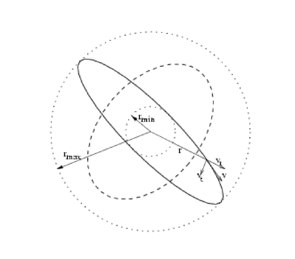
Figure 2: The sketch shows a typical orbit (dashed curve) of a dwarf spheroidal galaxy around the Milky Way, and defines the various distances and velocities used in the calculation. It is assumed that all the permitted orbits of dSphs lie between $r_{\rm min}$ and $r_{\rm max}$ (see text). The solid curve represents the “maximal” orbit: This orbit has the maximum transverse velocity at $r_{\rm min}$ and hence permits the maximum radial velocity at any $r$.

Now, referring to Figure 2 we can write the equations for the conservation of energy and angular momentum of a dSph’s motion as

$$E=\frac{1}{2}(v_{r}^{2}+v_{t}^{2})+\phi\,,$$ (5)

and

$$J=rv_{t}=r_{\rm min}v_{t}(r_{\rm min})=r_{\rm min}\sqrt{2[E-\phi(r_{\rm min})]}\,,$$ (6)

where $E$ is the energy per unit mass, $J$ the angular momentum per unit mass, $v_{t}$ the transverse velocity and $\phi$ is total gravitational potential of the Galaxy.

Manipulating equations (5), (6) we can write

$$v_{t}^{2}(r)=\frac{r^{2}_{\rm min}}{r^{2}-r^{2}_{\rm min}}\left\{v_{r}^{2}(r)+2[\phi(r)-\phi(r_{\rm min})]\right\}\,.$$ (7)

The spatial restriction imposed on the orbits by equation (4) implies constraints on the velocity components $v_{r}$ and $v_{t}$, which can be deduced as follows: First, note that the orbit having the maximum transverse velocity at $r_{\rm min}$ will be the one that permits the maximum radial velocity at any $r$. Considering this “maximal” orbit, shown schematically in Figure 2, and using the energy and angular momentum conservation equations given above, it is easy to show that the maximum radial velocity, $v_{r,{\rm max}}$, at any $r$ is given by

$$v^{2}_{r,{\rm max}}(r)=2\left(\frac{r^{2}_{\rm max}}{r^{2}_{\rm max}-r^{2}_{\rm min}}\right)\left(\frac{r^{2}-r^{2}_{\rm min}}{r^{2}}\right)\left[\phi(r_{\rm max})-\phi(r_{\rm min})\right]-2\left[\phi(r)-\phi(r_{\rm min})\right]\,.$$ (8)

The maximum $v_{t}$ at any $r\,$, $v_{t,{\rm max}}\left(r,v_{r}(r)\right)$, using conservation of energy, is then given by

$$v^{2}_{t,{\rm max}}\left(r,v_{r}(r)\right)=\frac{r^{2}_{\rm max}}{r^{2}_{\rm max}-r^{2}}\left\{2\left[\phi(r_{\rm max})-\phi(r)\right]-v_{r}^{2}(r)\right\}\,.$$ (9)

It can be shown by a Taylor expansion around $r=r_{\rm max}$, that this equation (9) correctly gives $v^{2}_{t,{\rm max}}(r\to r_{\rm max})=r\frac{\partial\phi}{\partial r}|_{r_{\rm max}}=v_{c}^{2}(r_{\rm max})$, where $v_{c}$ is the circular velocity.

The minimum $v_{t}$ at $r\,$, $v_{t,{\rm min}}\left(r,v_{r}(r)\right)$, has to be such that the radial velocity at $r_{\rm min}$ for this orbit, $v_{r}\left(r_{\rm min}\,,v_{r}(r)\right)\,$, vanishes, and the kinetic energy at $r_{\rm min}$ is completely due to transverse motion. This gives

$$v^{2}_{t,{\rm min}}\left(r,v_{r}(r)\right)=\frac{r^{2}_{\rm min}}{r^{2}-r^{2}_{\rm min}}\left\{v_{r}^{2}(r)+2\left[\phi(r)-\phi(r_{\rm min})\right]\right\}\,.$$ (10)

Notice, as before, $v^{2}_{t,{\rm min}}(r\to r_{\rm min})=v_{c}^{2}(r_{\rm min})$.

Figure 3: Constraints on the radial and transverse velocities of dSphs given by equations (8), (9) and (10) displayed as functions of $r$ for $r_{\rm min}=50\,{\rm kpc}$ and $r_{\rm max}=250\,{\rm kpc}$, for the “softened Keplerian” potential of the form $\phi(r)=-\kappa\left(1+(r/r_{0})\right)^{-1}$ with normalizations $\kappa\sim 40\times(100\,{\rm km}\,{\rm s}^{-1})^{2}$ and $r_{0}\sim 65\,{\rm kpc}$. The $v^{2}_{t,{\rm min}}(r,v_{r}(r))$ (solid curves) and $v^{2}_{t,{\rm max}}(r,v_{r}(r))$ (dashed curves) are shown for five different values of $v_{r}^{2}(r)$, namely, $v_{r}^{2}(r)=(0.2,0.4,0.6,0.8,1)\times v^{2}_{r,{\rm max}}(r)$ (from top to bottom). The dotted curve shows $v^{2}_{r,{\rm max}}(r)$. Similar constraints derived from a self-consistent model of the Galaxy were used for deriving the results quoted in the paper.

The constraint equations (8), (9) and (10) as functions of $r$ are displayed for illustration in Figure 3 for a simple representative Galactic potential at large $r$ of the form

$$\phi(r)=-\kappa\left(1+(r/r_{0})\right)^{-1}\,,$$ (11)

where $\kappa$ and $r_{0}$ are dimensionful constants. We have found that this simple “softened Keplerian” potential with appropriately chosen values of the normalization constants, $\kappa\sim 40\times(100\,{\rm km}\,{\rm s}^{-1})^{2}$ and $r_{0}\sim 65\,{\rm kpc}$ roughly reproduces the potential of the Galaxy at large galactocentric distances $\raise 1.29167pt\hbox{$\;>$\kern-7.5pt\raise-4.73611pt\hbox{$\sim\;$}}50\,{\rm kpc}$. Notice that $v^{2}_{r,{\rm max}}$ vanishes at $r_{\rm min}$ and $r_{\rm max}$ and is less than $v^{2}_{t,{\rm max}}$ for considerable distances from the end points, and it is only at intermediate distances that $v^{2}_{r,{\rm max}}$ becomes larger than $v^{2}_{t,{\rm min}}$ and $v^{2}_{t,{\rm max}}$ for large values of $v_{r}$. Thus it is clear that such kinematic restrictions on the population will yield one with a large value of the asymmetry parameter $j$ defined in equation (1). We should emphasize that the choice of the potential (11) here is merely to illustrate the general nature of the constraint equations. In the actual calculations and the results presented in this paper the potential is calculated self-consistently using a dynamical model of the Galaxy described in section 5.

The kinematic constraints derived above will immediately impose asymmetries on the phase space distribution function of the dSphs. Writing the primitive isotropic phase space distribution function of the dSphs as $F(v_{t},v_{r},r)$, the spatial number density distribution of the dSphs is given by

$$n(r)=\int_{0}^{v_{r,{\rm max}}}\int_{v_{t,{\rm min}}}^{v_{t,{\rm max}}}F(v_{t},v_{r},r)\,\,2\pi\,\,v_{t}\,\,dv_{t}\,\,dv_{r}\,,$$ (12)

for $r_{\rm min}<r<r_{\rm max}$, and $n(r)=0$ otherwise. The radial number distribution $N(r)$ of the dSphs is then given by equation (2).

Similarly the velocity skewness or asymmetry parameter $j$ defined in equation (1) is given by

$$j=\frac{\int_{r_{\rm min}}^{r_{\rm max}}\int_{0}^{v_{r,{\rm max}}}\int_{v_{t,{\rm min}}}^{v_{t,{\rm max}}}F(v_{t},v_{r},r)v^{2}\,\,2\pi\,\,v_{t}\,\,dv_{t}\,\,dv_{r}\,\,d^{3}r}{\int_{r_{\rm min}}^{r_{\rm max}}\int_{0}^{v_{r,{\rm max}}}\int_{v_{t,{\rm min}}}^{v_{t,{\rm max}}}F(v_{t},v_{r},r)v_{r}^{2}\,\,2\pi\,\,v_{t}\,\,dv_{t}\,\,dv_{r}\,\,d^{3}r}\,.$$ (13)

Before we calculate these constrained distributions and the skewness parameter from a self-consistent dynamical model, we will discuss the importance of the skewness parameter $j$ in constraining the circular speed and in turn the Galactic potential at large distances.

4 Circular rotation speed at large Galactocentric distances

The estimate of the skewness parameter $j$ from the observed data allows us to derive the circular rotation speeds $v_{c}$ in the Galactic potential at distances spanned by the dSphs. Following Lynden-Bell and Frenk (1981) consider the identity

$$\frac{1}{2}\frac{d^{2}|\mbox{\boldmath$r$}|^{2}}{dt^{2}}-{\mbox{\boldmath$v$}}^{2}=\mbox{\boldmath$r$}.\ddot{\mbox{\boldmath$r$}}=\mbox{\boldmath$r$}.\mbox{\boldmath$\nabla$}\phi=-v_{c}^{2}\,,$$ (14)

applicable to any particle moving in a gravitational potential $\phi$. Here $\mbox{\boldmath$v$}=\dot{\mbox{\boldmath$r$}}$ denotes the velocity vector of a particle at the position $r$ with respect to the center, and $v_{c}(r)$ is the circular velocity that would balance the radial component of gravity at the radius $r$. Averaging equation (14) over an ensemble of particles with position vectors $r_{i}$ and noting that

$$\frac{d}{dt}\sum_{i}\mbox{\boldmath$r_{i}$}^{2}=\frac{dI}{dt}=0\,$$ (15)

for a system of particles in virial equilibrium ($I$ being the moment of inertia), one gets

$$\langle v^{2}\rangle=\langle v_{c}^{2}\rangle\,.$$ (16)

Thus, by measuring $\langle v^{2}\rangle$ for an ensemble of objects at large Galactocentric distances we may estimate the value of $\langle v_{c}^{2}\rangle$ at those distances. As emphasized by Lynden-Bell and Lynden-Bell (1995), the validity of this theorem does not require that the potential be self-generated by the ensemble of particles under consideration. Thus, in general, we can write,

$$\langle v_{c}^{2}\rangle=j\langle v_{r}^{2}\rangle\,,\,\,\,{\rm or}\,\,v_{c}\sim j^{1/2}\langle v_{r}^{2}\rangle^{1/2}\,.$$ (17)

It is worth emphasizing that in this formulation of the virial theorem the kinetic energy gets equated to $\langle r\partial\phi/\partial r\rangle$ rather than to the potential energy as in the standard formulation.

The root mean square of the radial velocities, $\langle v_{r}^{2}\rangle^{1/2}$, can be estimated from a compilation of the radial velocities of various astronomical objects given in Table 2 and 3 of WE99, for example. This gives $\langle v_{r}^{2}\rangle^{1/2}\sim 115\,{\rm km}\,{\rm s}^{-1}$. The errors we expect in the determination of this $\langle v_{r}^{2}\rangle^{1/2}$ are primarily systematic, even though the smallness of the sample will also contribute to the uncertainties. Referring to the extensive review by Mateo (1998) we note that the typical accuracy with which the radial velocities with respect to the solar system barycentre are quoted is $\pm 2\,{\rm km}\,{\rm s}^{-1}$. Thus the errors are primarily due to the uncertainty in the circular velocity of the local standard of rest. Keeping in mind that the value of the circular rotation velocity at solar circle quoted in literature is in the range 200 – 220 $\,{\rm km}\,{\rm s}^{-1}$, and that the component of this velocity in the direction of the satellite is to be subtracted from the observed radial velocity with respect to the solar system, there would be an additional uncertainty of $\sim 5\,{\rm km}\,{\rm s}^{-1}$ on the average in the estimate of $\langle v_{r}^{2}\rangle^{1/2}$.

The measurements of proper motions are less certain and provide estimates of the transverse velocities as seen from the solar system. Since the solar system is at a distance of $\sim 8.5\,{\rm kpc}$ from the Galactic centre we need to make use of both the observed components of the velocities to determine the radial velocity with respect to the Galactic centre. In so far as the distances of the satellites are much larger than 8.5 kpc, the transformations of the velocity components from the heliocentric to the Galactocentric system do not add additional uncertainties except in rare instances. Thus the determination of $\langle v_{r}^{2}\rangle^{1/2}$ is reasonably robust.

On the other hand, the transverse velocities are to be estimated from the measurements of proper motions and are subject to greater uncertainties. This, coupled with the fact that there are only a small number of dSphs for which proper motion data are available, makes reliable observational determination of the anisotropy parameter $j$ from direct measurements of the radial and transverse velocities somewhat difficult. We shall instead estimate the parameter $j$ in section 8 below from the observed radial number distribution, $N(r)$, of the dSphs, which was introduced in section 2.

To proceed further, we next describe the model we have adopted for calculating the potential of the Galaxy in which the dSphs move.

5 Dynamical Model for the Dark Matter Halo of the Galaxy: The mathematical formalism

Both the visible matter and the dark matter contribute to the potential of the Galaxy, even though their relative contributions vary, with visible matter dominating at galactocentric distances below $\sim 5\,{\rm kpc}$ and the dark matter contribution increasing slowly with distance until beyond $\sim 20\,{\rm kpc}$ it is the dominant contributor. Whereas the density distribution of visible matter may be directly inferred from the astronomical observations, the density distribution of dark matter has to be deduced by somewhat more involved methods. The spatial distribution of the DM particles is dictated by their velocity distribution and the overall gravitational potential to which they also contribute depending on their density distribution. Thus one should ensure internal consistency between their velocity distribution and their density whose contribution to the potential when added to that of the visible matter should yield the overall potential.

The overall gravitational potential of the Galaxy is well determined by the observed rotation curve of the Galaxy at least up to $\sim$ 15 kpc. The method using the dSphs discussed in the previous section will help us to determine the potential up to distances of $\sim$ 100 – 200 kpc. In order to ensure the overall self-consistency we need a dynamical model, and to this end we start by making a convenient ansatz regarding the functional form of the phase space distribution of the particles constituting the DM halo. We then derive the structure of the halo by solving the combined Poisson-Boltzmann equation which involves the known gravitational potential of the visible matter of stars and gas of the Galaxy and the as yet undetermined potential of the DM halo. The solutions are a parametrized family of functions representing the potential due to the dark matter distribution. We may add to this the known contribution of the visible matter to get the total potential corresponding to different values of the parameters that characterize our DM halo model. By fitting the potential derived from the measurements of the rotation curve and the dSph dynamics, we can then determine the acceptable range of the parameters of our assumed DM halo model.

We assume that the density distribution of the normal visible matter is known and can be described adequately by a spheroidal bulge superposed on an axisymmetric disc (Caldwell and Ostriker, 1981; Binney and Tremaine, 1987; Kuijken and Gilmore, 1989). The density distributions of these are given respectively by

$$\rho_{s}(r)=\rho_{s}(0)\left(1+\frac{r^{2}}{a^{2}}\right)^{-3/2}\,,$$ (18)

and

$$\rho_{d}(r)=\frac{\Sigma}{2h}e^{-(R-R_{0})/R_{d}}\,\,\,e^{-|z|/h}\,,$$ (19)

where $r=(R^{2}+z^{2})^{1/2}\,$, $R$ being the Galactocentric distance in the median plane of the disc and $z$ the distance normal to the plane. The parameters take the values $\rho_{s}(0)=4.2\times 10^{2}\,{\rm M}_{\odot}\,{\rm pc}^{-3}\,\,$, $a=0.103\,{\rm kpc}\,$, $R_{d}=3.5\,{\rm kpc}\,$, and $h=0.3\,{\rm kpc}\,$. Also $R_{0}=8.5\,{\rm kpc}\,$ is the solar Galactocentric distance and $\Sigma\approx 36\,{\rm M}_{\odot}\,{\rm pc}^{-2}$ is the column density of the disk at the solar location. The expressions for the gravitational potentials, $\phi_{s}$ and $\phi_{d}$, corresponding to above forms of $\rho_{s}$ and $\rho_{d}$, are given in Caldwell and Ostriker (1981) and Kuijken and Gilmore (1989).

The true phase space DF that describes the DM halo of the Galaxy is not known. To make progress we choose a phase-space distribution function (DF) of the dark matter dictated by the following physical considerations: It should represent a collisionless system and should allow a parametrization in terms of the three main physical parameters of the halo, namely, the density and velocity dispersion of dark matter at some reference location within the halo, and the size (radius) of the halo. The truncated or the so-called “lowered” isothermal distribution (often called the “King” model) is a simple DF which has these features, and has been studied extensively (see, e.g., Binney and Tremaine, 1987, p. 232). As such, in the present study we adopt this DF, which is given by

$$f(x,v)\equiv f(\varepsilon)=\left\{\begin{array}[]{ll}\rho_{1}(2\pi\sigma^{2})^{-3/2}\left(e^{\varepsilon/\sigma^{2}}-1\right)&\mbox{for $\varepsilon>0$}\,,\\ 0&\mbox{for $\varepsilon\leq 0$}\,,\end{array}\right.$$ (20)

with

$$\varepsilon\equiv\phi_{0}-(\frac{1}{2}v^{2}+\phi)\,.$$ (21)

Here $\phi=\phi_{s}+\phi_{d}+\phi_{\rm\scriptscriptstyle DM}$ is the total gravitational potential due to the visible and the dark matter components of the Galaxy, and $\phi_{0}$, $\rho_{1}$ and $\sigma$ are parameters to be determined by comparing the results of the model calculations with observations. Notice that here $f$ is chosen as a function of the conserved quantity, total energy (per unit mass), $E=(\frac{1}{2}v^{2}+\phi)$, so that the collisionless Boltzmann equation is stationary. The density of dark matter is given by

$$\rho_{\rm\scriptscriptstyle DM}=\int f\,\,d^{3}v\,,$$ (22)

and vanishes at the location $r=r_{t}$ where $\varepsilon=0$, representing the outer edge of the halo. Note also that the parameter $\sigma$ (having the dimension of velocity) is not equal to the velocity dispersion of the DM particles, $\langle v^{2}\rangle^{1/2}_{\rm\scriptscriptstyle DM}$; the latter can be calculated for the DF given above and is a function of $r$, vanishing at $r=r_{t}$.

The visible matter potentials and densities being already known, the DM potential $\phi_{\rm\scriptscriptstyle DM}$ is obtained by solving the Poisson equation

$$\nabla^{2}\phi_{\rm\scriptscriptstyle DM}(R,z)=4\pi G\rho_{\rm\scriptscriptstyle DM}(R,z)\,.$$ (23)

Notice that $\rho_{\rm\scriptscriptstyle DM}$ appearing on the $r.h.s.$ of the equation (23) is a nonlinear functional of $\phi=\phi_{s}+\phi_{d}+\phi_{\rm\scriptscriptstyle DM}$ via equations (20), (21) and (22). Assuming axisymmetry, we numerically solve the nonlinear equation (23) through an iterative procedure discussed earlier in Cowsik et al. (1996), which has been tested on special cases where analytical solutions are available. The solutions thus obtained give the values of $\phi_{\rm\scriptscriptstyle DM}(R,z)$ for different chosen values of the parameters $\rho_{1},\sigma$ and $\phi_{0}$.

In our numerical calculations we take the DM density at the solar location, $\rho_{{\rm\scriptscriptstyle DM},\odot}=\rho_{\rm\scriptscriptstyle DM}(R=R_{0},0)$, the DM velocity dispersion at the solar location, $\langle v^{2}\rangle^{1/2}_{{\rm\scriptscriptstyle DM},\odot}=\langle v^{2}\rangle^{1/2}_{\rm\scriptscriptstyle DM}(R=R_{0},0)$, and the truncation radius $r_{t}$, as the three “observable” free parameters of the model, instead of the parameters $\rho_{1}$, $\sigma$ and $\phi_{0}$ appearing in equations (20) and (21). From this 3-parameter family of solutions we need to choose the one which fits all the known observations.

6 The Rotation Curve and the value of $\rho_{{\rm\scriptscriptstyle DM},\odot}$

One of the most useful probes of the potential of the Galaxy is the circular rotation curve (RC), $v_{c}(R)$, which is given by

$$v_{c}^{2}(R)=R\frac{\partial\phi}{\partial R}(R,0)=R\frac{\partial}{\partial R}\left[\phi_{\rm\scriptscriptstyle DM}(R,0)+\phi_{s}(R,0)+\phi_{d}(R,0)\right]\,.$$ (24)

Figure 4: A sample of theoretically calculated rotation curves of the Galaxy based on our self-consistent model, including the lower bounds derived from the study of dynamics of dwarf spheroidals. The dark matter is modeled as having a lowered (truncated) isothermal distribution. The curves shown are for dark matter density in the solar neighborhood, $\rho_{{\rm\scriptscriptstyle DM},\odot}\approx 0.3\,{\rm GeV}\,{\rm cm}^{-3}$, truncation radius, $r_{t}=150\,{\rm kpc}$, and various values of $\langle v^{2}\rangle^{1/2}_{{\rm\scriptscriptstyle DM},\odot}$, the velocity dispersion of the dark matter particles at the solar neighborhood, as indicated. The solid curve corresponds to the maximum possible value of $\langle v^{2}\rangle^{1/2}_{{\rm\scriptscriptstyle DM},\odot}$ consistent with the chosen values of $\rho_{{\rm\scriptscriptstyle DM},\odot}$ and $r_{t}$. The doubly thick solid curve represents our “conservative most likely” (CML) model (see text) with DM parameter values $\rho_{{\rm\scriptscriptstyle DM},\odot}\approx 0.3\,{\rm GeV}\,{\rm cm}^{-3}$, $\langle v^{2}\rangle^{1/2}_{{\rm\scriptscriptstyle DM},\odot}\approx 400\,{\rm km}\,{\rm s}^{-1}$ and $r_{t}=200\,{\rm kpc}$. The observational data (crosses and vertical lines with error bars) are from Honma and Sofue (1997) for the case $R_{0}=8\,{\rm kpc}$ and $v_{c}(R=R_{0})=200\,{\rm km}\,{\rm s}^{-1}$. The two solid horizontal lines represent two different estimates of the expected lower limits on $v_{c}$ in the region of $R\sim 100\,{\rm kpc}$ obtained in this paper from the dynamics of the dwarf spheroidals. The small glitches in the curves at $R\simeq 100\,{\rm kpc}$ are artifacts of numerical calculation and are due to increased grid spacing used for distances $r\geq 100\,{\rm kpc}$ in order to reduce the total computation time.

We have run a series of models of the Galaxy spanning a wide range of values of the parameters $\rho_{{\rm\scriptscriptstyle DM},\odot}$, $\langle v^{2}\rangle^{1/2}_{{\rm\scriptscriptstyle DM},\odot}$ and $r_{t}$ distributed about their values estimated from earlier studies. Figure 4 shows a sample of the RC’s of the Galaxy calculated from our model  together with the available data for $R\raise 1.29167pt\hbox{$\;<$\kern-7.5pt\raise-4.73611pt\hbox{$\sim\;$}}20\,{\rm kpc}$ as summarized in Honma and Sofue (1997). In the same Figure we have also indicated two different estimates of the expected lower limits on $v_{c}$ in the region $R\sim 100\,{\rm kpc}$ obtained in this paper from the dynamics of the dwarf-spheroidals; derivation of these estimates is discussed in section 8 below.

In the very central regions ($R\raise 1.29167pt\hbox{$\;<$\kern-7.5pt\raise-4.73611pt\hbox{$\sim\;$}}1\,{\rm kpc}$) of the Galaxy the density of normal matter is so high that the RC is essentially determined by it and is sensibly independent of the parameters of the DM. In the region $1\,{\rm kpc}<R\raise 1.29167pt\hbox{$\;<$\kern-7.5pt\raise-4.73611pt\hbox{$\sim\;$}}10\,{\rm kpc}$ the contribution of normal matter progressively decreases as the contribution of DM increases, maintaining a nearly flat RC. Based on the results of our extensive calculations of approximately more than two hundred model RCs for a wide range of the relevant parameters (only a selected few of which are shown in Fig. 4, Fig. 12 and Fig. 13), we can conclude that, as long as we restrict ourselves to the available data below galactocentric distances of $\sim 20\,{\rm kpc}$, a range of $\rho_{{\rm\scriptscriptstyle DM},\odot}$ values from $\sim 0.25\,{\rm GeV}/\,{\rm cm}^{3}$ to $\sim 0.4\,{\rm GeV}/\,{\rm cm}^{3}$ with suitably chosen values of the other two parameters, $r_{t}$ and $\langle v^{2}\rangle^{1/2}_{{\rm\scriptscriptstyle DM},\odot}$, can yield acceptable fits to the data. To be specific, we use the value

$$\rho_{{\rm\scriptscriptstyle DM},\odot}\approx 0.3\,{\rm GeV}\,{\rm cm}^{-3}\,$$ (25)

for the DM density in the solar neighborhood in our numerical calculations discussed below; the results derived in this paper do not change by any significant amount for other values of this parameter within the approximate range given above. Some theoretical rotation curves for other values of $\rho_{{\rm\scriptscriptstyle DM},\odot}$ are given in Appendix A.

Sensitivity of the rotation curves to the two other parameters of our DM halo model, namely, $r_{t}$ and $\langle v^{2}\rangle^{1/2}_{{\rm\scriptscriptstyle DM},\odot}$, commences at distances $R>10\,{\rm kpc}$, with strong sensitivity to these parameters at $R>20\,{\rm kpc}$ where direct measurements of the rotation curve are absent. The estimates of the rotation speeds derived from the dynamics of dSphs, therefore, play an important role in constraining the values of these two parameters, which we shall proceed to discuss in the next section.

Based on the nature of the theoretical rotation curves displayed in Fig. 4, Fig. 12 and Fig. 13, for example, together with the existing rotation curve data, we shall restrict our attention, for the subsequent discussions in the paper, to the values of the parameters $r_{t}$ and $\langle v^{2}\rangle^{1/2}_{{\rm\scriptscriptstyle DM},\odot}$ satisfying

$$r_{t}\geq 100\,{\rm kpc}\,,$$ (26)

and

$$\langle v^{2}\rangle^{1/2}_{{\rm\scriptscriptstyle DM},\odot}\geq 300\,{\rm km}\,{\rm s}^{-1}\,.$$ (27)

For suitable choices of values of the parameters in these ranges, the theoretical rotation curves fit the observed data satisfactorily. Some theoretical rotation curves for parameter values outside the values and ranges indicated by equations (25), (26) and (27) are also shown in Fig. 4, Fig. 12 and Fig. 13.

The DM density profiles in the plane of the Galaxy for the same set of our self-consistent models corresponding to the rotation curves of Fig. 4 are shown in Figure 5.

Figure 5: The dark matter density profiles in the plane of the Galaxy for the same set of model parameters corresponding to the rotation curves of Fig. 4.

7 Constraining the parameters of the dark matter halo using the dynamics of dwarf spheroidals

As discussed in Section 4 the rotation speeds at large galactocentric distances can be estimated from the dynamics of the dSphs. In sections 2 and 3 it was shown that the dSphs will have a skewness in their velocity distribution quantified in terms of the parameter $j$, which is a sensitive function of the parameter $r_{\rm min}$, the location of the dip in the radial number distribution of the satellites of the Galaxy. We can determine the value of $r_{\rm min}$, and hence, the parameter $j$, from the observed radial distribution of the dSphs in the following way.

Referring to Fig. 1, let $N_{i}^{\rm obs}$ be the observed number of dSphs in the $i$-th, 10 kpc-size radial distance bin, with $i=1,2,\ldots$ denoting the radial distance bins (0–10 kpc), (10–20 kpc), etc., respectively. We calculate the theoretical expectation for the number of objects in each of these bins, $N_{i}^{\rm th}$, from the radial number distribution of the satellites, $N(r)$, calculated in a number of theoretical models with various possible values of $r_{\rm min}$ and a large enough value of $r_{\rm max}\approx 500\,{\rm kpc}$. Our calculations discussed below have negligible dependence on the exact value of $r_{\rm max}$ as long as it is large enough to accommodate the most distant satellites.

The radial number distribution $N(r)$ can be calculated using equations (2) and (12). To do this, we need to provide the primitive (undistorted) phase space distribution function, $F(v_{t},v_{r},r)$, of the satellites, which we take to be of isothermal form, namely,

$$F(v_{t},v_{r},r)\propto\exp\left\{-3\left(\frac{1}{2}(v_{r}^{2}+v_{t}^{2})+\phi(r)\right)/\sigma^{2}_{s}\right\}\,,$$ (28)

where $\sigma_{s}$ is the primitive velocity dispersion of the satellites, and $\phi(r)$ is the gravitational potential in which the satellites move . The potential can be taken to be spherically symmetric without much loss of accuracy since our theoretically calculated self-consistent potentials become progressively spherically symmetric at the large galactocentric distances where the dSphs lie. The kinematic velocity limits appearing in equation (12) are obtained by solving the constraint equations (8), (9) and (10) for a given self-consistent potential $\phi(r)$ and given values of $r_{\rm min}$ and $r_{\rm max}$.

Having already fixed the DM halo model parameter $\rho_{{\rm\scriptscriptstyle DM},\odot}$, we can numerically calculate the theoretical quantities $N_{i}^{\rm th}$ for plausible values of the other relevant parameters, namely, $r_{t}$, $\langle v^{2}\rangle^{1/2}_{{\rm\scriptscriptstyle DM},\odot}$, $\sigma_{s}$ and $r_{\rm min}$, and determine the most likely values of these parameters by performing a simple likelihood analysis as follows: Assuming Poissonian probability distribution,

$$P_{i}\left(N_{i}^{\rm obs},N_{i}^{\rm th}\right)=e^{-N_{i}^{\rm th}}\left(N_{i}^{\rm th}\right)^{N_{i}^{\rm obs}}\frac{1}{N_{i}^{\rm obs}!}\,,$$ (29)

for the occurrence of $N_{i}^{\rm obs}$ number of dSphs in the $i$-th radial bin when the expectation is $N_{i}^{\rm th}$, we calculate the likelihood function ${\mathcal{L}}$ defined as

$${\mathcal{L}}\equiv\frac{\prod_{i=1}^{i_{\rm max}}P_{i}\left(N_{i}^{\rm obs},N_{i}^{\rm th}\right)}{\prod_{i=1}^{i_{\rm max}}P_{i}\left(N_{i}^{\rm obs},N_{i,{\rm B}}^{\rm th}\right)}=\prod_{i=1}^{i_{\rm max}}e^{-\left(N_{i}^{\rm th}-N_{i,{\rm B}}^{\rm th}\right)}\left(\frac{N_{i}^{\rm th}}{N_{i,{\rm B}}^{\rm th}}\right)^{N_{i}^{\rm obs}}\,,$$ (30)

where $i_{\rm max}$ denotes the maximum number of radial bins and $N_{i,{\rm B}}^{\rm th}$ is the mean number expected in the $i$-th bin calculated in a base model with fixed values of the parameters $r_{t}$, $\langle v^{2}\rangle^{1/2}_{{\rm\scriptscriptstyle DM},\odot}$, $\sigma_{s}$ and $r_{\rm min}$.

Note that, depending on the value of $r_{\rm min}$ for the model under consideration, there will be bins with $r<r_{\rm min}$ for which $N_{i,{\rm B}}^{\rm th}$ or both $N_{i,{\rm B}}^{\rm th}$ and $N_{i}^{\rm th}$ may be zero, in which cases ${\mathcal{L}}$ defined in equation (30) diverges or is ill-defined. This, of course, is an artifact, due to the sharp cut-off in the number distribution of the satellites at $r_{\rm min}$. A more mathematically rigorous procedure would be to impose, for example, an exponential cutoff of the number distribution of the satellites below $r_{\rm min}$, thus giving a small but finite number for the values of $N_{i,{\rm B}}^{\rm th}$ and $N_{i}^{\rm th}$ below $r_{\rm min}$. Another way to avoid the problem is to use the simple regularization procedure of adding a small constant $\epsilon$ to $N_{i}^{\rm th}$ in the numerical calculations of ${\mathcal{L}}$, which is the procedure we have followed in our calculations of ${\mathcal{L}}$. We have checked that the resulting numerical values of $\mathcal{L}$ have negligible sensitivity to the assumed value of $\epsilon$ in the range $\epsilon\sim 10^{-6}$ – $10^{-4}$. Accordingly, we take $\epsilon=10^{-6}$ in our numerical calculations.

Figure 6: The likelihood $\mathcal{L}$ as a function of the parameter $r_{\rm min}$ for various different values of $\sigma_{s}$ as indicated, for fixed values of $r_{t}=200\,{\rm kpc}$, $\rho_{{\rm\scriptscriptstyle DM},\odot}=0.3\,{\rm GeV}/\,{\rm cm}^{3}$ and $\langle v^{2}\rangle^{1/2}_{{\rm\scriptscriptstyle DM},\odot}=400\,{\rm km}\,{\rm s}^{-1}$. The base model has the parameter values $r_{t}=200\,{\rm kpc}$, $\rho_{{\rm\scriptscriptstyle DM},\odot}=0.3\,{\rm GeV}/\,{\rm cm}^{3}$, $\langle v^{2}\rangle^{1/2}_{{\rm\scriptscriptstyle DM},\odot}=400\,{\rm km}\,{\rm s}^{-1}$, $\sigma_{s}=180\,{\rm km}\,{\rm s}^{-1}$ and $r_{\rm min}=61\,{\rm kpc}$.

7.1 Likelihood of model parameters

We have calculated the likelihood function $\mathcal{L}$ for a wide range of plausible values of the relevant parameters. Of the parameters $r_{t}$, $\langle v^{2}\rangle^{1/2}_{{\rm\scriptscriptstyle DM},\odot}$, $\sigma_{s}$ and $r_{\rm min}$, the most sensitive dependence of $\mathcal{L}$ is on $r_{\rm min}$. In Figures 6 and 7 we display the result of our calculation of $\mathcal{L}$ as a function of the parameter $r_{\rm min}$ for various different values of $\sigma_{s}$ and for two fixed sets of values of the DM model parameters, namely, $\rho_{{\rm\scriptscriptstyle DM},\odot}=0.3\,{\rm GeV}/\,{\rm cm}^{3}$, $\langle v^{2}\rangle^{1/2}_{{\rm\scriptscriptstyle DM},\odot}=400\,{\rm km}\,{\rm s}^{-1}$ and $r_{t}=200\,{\rm kpc}$ (Fig. 6), and $\rho_{{\rm\scriptscriptstyle DM},\odot}=0.3\,{\rm GeV}/\,{\rm cm}^{3}$, $\langle v^{2}\rangle^{1/2}_{{\rm\scriptscriptstyle DM},\odot}=400\,{\rm km}\,{\rm s}^{-1}$ and $r_{t}=150\,{\rm kpc}$ (Fig. 7).

Figure 7: The likelihood $\mathcal{L}$ as a function of the parameter $r_{\rm min}$ for various different values of $\sigma_{s}$ as indicated, for fixed values of $r_{t}=150\,{\rm kpc}$, $\rho_{{\rm\scriptscriptstyle DM},\odot}=0.3\,{\rm GeV}/\,{\rm cm}^{3}$ and $\langle v^{2}\rangle^{1/2}_{{\rm\scriptscriptstyle DM},\odot}=400\,{\rm km}\,{\rm s}^{-1}$. The base model has the parameter values $r_{t}=200\,{\rm kpc}$, $\rho_{{\rm\scriptscriptstyle DM},\odot}=0.3\,{\rm GeV}/\,{\rm cm}^{3}$, $\langle v^{2}\rangle^{1/2}_{{\rm\scriptscriptstyle DM},\odot}=400\,{\rm km}\,{\rm s}^{-1}$, $\sigma_{s}=180\,{\rm km}\,{\rm s}^{-1}$ and $r_{\rm min}=61\,{\rm kpc}$.

The dependence of the likelihood of different models on the value of the parameter $\langle v^{2}\rangle^{1/2}_{{\rm\scriptscriptstyle DM},\odot}$ is illustrated in Figure 8 where we display $\mathcal{L}$ as a function $r_{\rm min}$ for fixed values of $r_{t}=200\,{\rm kpc}$ and $\sigma_{s}=180\,{\rm km}\,{\rm s}^{-1}$ but for different values of the DM parameter $\langle v^{2}\rangle^{1/2}_{{\rm\scriptscriptstyle DM},\odot}$.

Figure 8: The likelihood $\mathcal{L}$ as a function of the parameter $r_{\rm min}$ for various different values of $\langle v^{2}\rangle^{1/2}_{{\rm\scriptscriptstyle DM},\odot}$ as indicated, for fixed values of $r_{t}=200\,{\rm kpc}$, $\rho_{{\rm\scriptscriptstyle DM},\odot}=0.3\,{\rm GeV}/\,{\rm cm}^{3}$ and $\sigma_{s}=180\,{\rm km}\,{\rm s}^{-1}$. The base model has the parameter values $r_{t}=200\,{\rm kpc}$, $\rho_{{\rm\scriptscriptstyle DM},\odot}=0.3\,{\rm GeV}/\,{\rm cm}^{3}$, $\langle v^{2}\rangle^{1/2}_{{\rm\scriptscriptstyle DM},\odot}=400\,{\rm km}\,{\rm s}^{-1}$, $\sigma_{s}=180\,{\rm km}\,{\rm s}^{-1}$ and $r_{\rm min}=61\,{\rm kpc}$.

The base model used in the likelihood curves shown in Figures 6, 7 and 8 has been chosen to have the parameter values

$$r_{t}=200\,{\rm kpc}\,,\,\rho_{{\rm\scriptscriptstyle DM},\odot}=0.3\,{\rm GeV}/\,{\rm cm}^{3}\,,\,\langle v^{2}\rangle^{1/2}_{{\rm\scriptscriptstyle DM},\odot}=400\,{\rm km}\,{\rm s}^{-1}\,,$$ (31)

$$\sigma_{s}=180\,{\rm km}\,{\rm s}^{-1}\,,{\rm and}\,\,r_{\rm min}=61\,{\rm kpc}\,.$$ (32)

The reason for choosing this set of parameter values for the base model is clear from a comparison of Figures 6, 7 and 8, which shows that this model has the highest likelihood within the ranges of values of the relevant parameters considered in these Figures. We have also calculated the likelihood $\mathcal{L}$ for parameter values beyond their ranges displayed in Figures 6, 7 and 8. The likelihood can be higher than that for the base model chosen above if we allow $\langle v^{2}\rangle^{1/2}_{{\rm\scriptscriptstyle DM},\odot}>400\,{\rm km}\,{\rm s}^{-1}$. For example, with respect to the above chosen base model, and with other parameters being equal, we get $\mathcal{L}\approx 1.04$ for a model with $\langle v^{2}\rangle^{1/2}_{{\rm\scriptscriptstyle DM},\odot}\approx 450\,{\rm km}\,{\rm s}^{-1}$ and $\sigma_{s}\approx 220\,{\rm km}\,{\rm s}^{-1}$. We have not done a fine-grained scanning of the entire parameter space spanned by all the relevant parameters for $\langle v^{2}\rangle^{1/2}_{{\rm\scriptscriptstyle DM},\odot}>400\,{\rm km}\,{\rm s}^{-1}$, but our present calculations indicate that the model with the absolute highest likelihood, i.e., the “best-fit” model seems to correspond to a value of $\langle v^{2}\rangle^{1/2}_{{\rm\scriptscriptstyle DM},\odot}$ close to $\sim 500\,{\rm km}\,{\rm s}^{-1}$ with $\sigma_{s}\sim 290\,{\rm km}\,{\rm s}^{-1}$. However, to be on the conservative side as far as the most likely value of the important parameter $\langle v^{2}\rangle^{1/2}_{{\rm\scriptscriptstyle DM},\odot}$ is concerned, we shall refer to the above chosen base model with parameters given by equations (31) and (32) as our “conservative most likely” (CML) model. The radial distribution of the dSphs calculated using equations (2) and (12) for the parameter values corresponding to the above CML model is shown in Figure 9.

Figure 9: Distribution of the number of dwarf-spheroidals as a function of the distance from the Galactic centre. The prediction of our conservative most likely model, which corresponds to $\langle v^{2}\rangle^{1/2}_{{\rm\scriptscriptstyle DM},\odot}=400\,{\rm km}\,{\rm s}^{-1}$, $\sigma_{s}=180\,{\rm km}\,{\rm s}^{-1}$ and $r_{\rm min}=61\,{\rm kpc}$, with $\rho_{{\rm\scriptscriptstyle DM},\odot}=0.3\,{\rm GeV}/\,{\rm cm}^{3}$ and $r_{t}=200\,{\rm kpc}$, is also shown (see also Fig. 1).

From Figures 6, 7 and 8, we find that the relevant parameter values outside the ranges

$$\langle v^{2}\rangle^{1/2}_{{\rm\scriptscriptstyle DM},\odot}\raise 1.29167pt\hbox{$\;>$\kern-7.5pt\raise-4.73611pt\hbox{$\sim\;$}}350\,{\rm km}\,{\rm s}^{-1}\,,\,\,150\raise 1.29167pt\hbox{$\;<$\kern-7.5pt\raise-4.73611pt\hbox{$\sim\;$}}r_{t}\raise 1.29167pt\hbox{$\;<$\kern-7.5pt\raise-4.73611pt\hbox{$\sim\;$}}200\,{\rm kpc}\,,$$ (33)

$$52\raise 1.29167pt\hbox{$\;<$\kern-7.5pt\raise-4.73611pt\hbox{$\sim\;$}}r_{\rm min}\raise 1.29167pt\hbox{$\;<$\kern-7.5pt\raise-4.73611pt\hbox{$\sim\;$}}66\,{\rm kpc}\,,\,\,150\raise 1.29167pt\hbox{$\;<$\kern-7.5pt\raise-4.73611pt\hbox{$\sim\;$}}\sigma_{s}\raise 1.29167pt\hbox{$\;<$\kern-7.5pt\raise-4.73611pt\hbox{$\sim\;$}}220\,{\rm km}\,{\rm s}^{-1}\,,\,$$ (34)

have less than 50% likelihood of explaining the observed radial distribution of the dSphs. Demanding higher likelihood narrows down these ranges further. Note that for the conservative most likely model the likelihood that $r_{\rm min}<50\,{\rm kpc}$ is very small, less than 4%.

8 Estimating the velocity anisotropy parameter $j$ and limits on the rotation speed at large galactocentric distances

We now have at hand all the parameters needed to theoretically estimate the value of $j$ using equation (13). To explicitly show the dependence of $j$ on $r_{\rm min}$ and $\sigma_{s}$, we have calculated $j$ as a function of $r_{\rm min}$ for various different values of $\sigma_{s}$, including very large values of $\sigma_{s}$ corresponding to a constant DF for the satellites. The results are shown in Figures 10 and 11 for $\langle v^{2}\rangle^{1/2}_{{\rm\scriptscriptstyle DM},\odot}=400\,{\rm km}\,{\rm s}^{-1}$, $r_{t}=200\,{\rm kpc}$ (Fig. 10) and $\langle v^{2}\rangle^{1/2}_{{\rm\scriptscriptstyle DM},\odot}=350\,{\rm km}\,{\rm s}^{-1}$, $r_{t}=150\,{\rm kpc}$ (Fig. 11).

Figure 10: The velocity anisotropy parameter $j$ as a function of $r_{\rm min}$ for various different values of $\sigma_{s}$ as indicated. The DM halo parameters have been fixed at $\rho_{{\rm\scriptscriptstyle DM},\odot}=0.3\,{\rm GeV}/\,{\rm cm}^{3}$, $\langle v^{2}\rangle^{1/2}_{{\rm\scriptscriptstyle DM},\odot}=400\,{\rm km}\,{\rm s}^{-1}$ and $r_{t}=200\,{\rm kpc}$.

Figure 11: Same as Fig. 10 but for $\langle v^{2}\rangle^{1/2}_{{\rm\scriptscriptstyle DM},\odot}=350\,{\rm km}\,{\rm s}^{-1}$ and $r_{t}=150\,{\rm kpc}$.

Note that, for a given potential $\phi(r)$ and a given value of $r_{\rm min}$, the lowest value of $j$ obtains, as expected, in the case $F=\,$ constant (i.e., $\sigma_{s}\to\infty$ in equation (28)), because then all orbits in the interval $r_{\rm min}$ to $r_{\rm max}$ will be equally probable. Smaller (finite) values of $\sigma_{s}$ correspond to favoring orbits with mean apogalacticons smaller than $(r_{\rm max}-r_{\rm min})/2$, making the orbits more circular and thus yielding larger values of $j$.

Considering the dependence of $j$ on the DM halo model parameters $\langle v^{2}\rangle^{1/2}_{{\rm\scriptscriptstyle DM},\odot}$ and $r_{t}$, we find that $j$ depends most sensitively on $\langle v^{2}\rangle^{1/2}_{{\rm\scriptscriptstyle DM},\odot}$ and weakly on $r_{t}$. In general, for a given value of $\langle v^{2}\rangle^{1/2}_{{\rm\scriptscriptstyle DM},\odot}$, the value of $j$ is smaller for a smaller value of $r_{t}$, but only marginally so for values of $r_{t}$ in the range 100 – 200 kpc.

From Figure 10 we find that for our CML model with the relevant parameter values given by equations (31) and (32), we get $j_{\rm CML}\approx 15.4$. The observational data on the dSphs given in WE99 yield $\langle v_{r}^{2}\rangle^{1/2}=116\,{\rm km}\,{\rm s}^{-1}$. Taking this to imply (conservatively) $\langle v_{r}^{2}\rangle^{1/2}\geq 100\,{\rm km}\,{\rm s}^{-1}$ one finds, using equation (17),

$$\langle v_{c}^{2}\rangle^{1/2}_{\rm CML}=j^{1/2}_{\rm CML}\langle v_{r}^{2}\rangle^{1/2}\raise 1.29167pt\hbox{$\;>$\kern-7.5pt\raise-4.73611pt\hbox{$\sim\;$}}392\,{\rm km}\,{\rm s}^{-1}\,.$$ (35)

This value is consistent to within about 15% with the peak value of the rotation curve for the DM model parameters corresponding to the CML model (indicated by the doubly thick solid curve in Figure 4).

To be conservative on the side of the asymmetry parameter $j$, if we take the parameter values $r_{\rm min}\geq 50\,{\rm kpc}$, $\sigma_{s}\leq 220\,{\rm km}\,{\rm s}^{-1}$, $\langle v^{2}\rangle^{1/2}_{{\rm\scriptscriptstyle DM},\odot}\geq 350\,{\rm km}\,{\rm s}^{-1}$ and $r_{t}\geq 150\,{\rm kpc}$, then we get $j_{\rm conservative}=8.2$, yielding

$$\langle v_{c}^{2}\rangle^{1/2}_{\rm conservative}\geq 286\,{\rm km}\,{\rm s}^{-1}$$ (36)

as a conservative estimate of the rotation speed at $r\sim$ 100–200 kpc, the typical distances of the dwarf spheroidals.

Even more conservatively, taking $\sigma_{s}\leq 280\,{\rm km}\,{\rm s}^{-1}$ with $r_{\rm min}\geq 50\,{\rm kpc}$, $\langle v^{2}\rangle^{1/2}_{{\rm\scriptscriptstyle DM},\odot}\geq 350\,{\rm km}\,{\rm s}^{-1}$ and $r_{t}\geq 150\,{\rm kpc}$, we get $j=7.1$, which yields

$$\langle v_{c}^{2}\rangle^{1/2}_{\rm most\,\,conservative}\geq 266\,{\rm km}\,{\rm s}^{-1}\,.$$ (37)

We have indicated the conservative lower limits (36) and (37) in Figures 4, 12 and 13 by the solid horizontal lines. Note that these lower limits on the rotation speeds are obtained entirely from the dynamics of the dSphs, and are clearly consistent with the rotation curves shown in Figures 4, 12 and 13 for $\langle v^{2}\rangle^{1/2}_{{\rm\scriptscriptstyle DM},\odot}>350\,{\rm km}\,{\rm s}^{-1}$ and $r_{t}>150\,{\rm km}\,{\rm s}^{-1}$.

In our analysis thus far in the estimation of $j$ we have assumed the DF of the dSphs to be isotropic at the epoch of their formation. In Appendix B we investigate the effects of making the initial DF favor radial velocities over transverse velocities. This analysis indicates that once the DF is modified by removing the subset of orbits with small perigalacticons, the resultant distribution function rapidly starts favoring transverse velocities. An intuitive understanding of the generation of anisotropies favoring transverse velocities as a result of imposing a minimum value on the perigalacticon radius may be gained through a kinematic analysis of elliptical orbits; this is presented in Appendix C.

From the foregoing analysis, supplemented by the discussions in the appendices A, B and C, we find that we are able to fit the available data on the rotation curve of the Galaxy, the radial distribution of the dwarf spheroidals and the value of the circular rotation speed at $\sim 100\,{\rm kpc}$ estimated from the analysis of the data on dSphs, with a self-consistent model of the Galactic dark matter halo in which the phase space distribution function of the DM particles is described by the King (i.e., the truncated isothermal) model, with the following values of the model parameters:

$$\begin{array}[]{rll}\rho_{{\rm\scriptscriptstyle DM},\odot}&\approx&0.3\,{\rm GeV}\,{\rm cm}^{-3}\,,\\ \langle v^{2}\rangle^{1/2}_{{\rm\scriptscriptstyle DM},\odot}&>&350\,{\rm km}\,{\rm s}^{-1}\,,\\ r_{t}&\raise 1.29167pt\hbox{$\;>$\kern-7.5pt\raise-4.73611pt\hbox{$\sim\;$}}&150\,{\rm kpc}\,.\\ \end{array}$$ (38)

Whereas we will have to await further astronomical observations to yield a complete, unbiased data set on the dSphs, it is expected that the above estimates, being conservative, will hold. The above estimates are also consistent with the earlier estimation of these parameters by Cowsik et al. (1996) using only the rotation curve data of the Galaxy up to $R\raise 1.29167pt\hbox{$\;<$\kern-7.5pt\raise-4.73611pt\hbox{$\sim\;$}}20\,{\rm kpc}$. The current set of parameters yields a total mass of the Galaxy, including its DM halo, $M_{\rm Galaxy}\sim 2\times 10^{12}\,{\rm M}_{\odot}$.

9 Summary and Conclusions

The theoretical density distribution of the dark matter particles constituting the halo depends sensitively on the competition between their velocity dispersion and the total gravitational potential generated by the dark and the baryonic matter of the Galaxy. We have exploited this sensitivity to estimate the parameters related to the phase space distribution of the dark matter in the Galaxy. This is carried out within the context of a self-consistent model of the dark matter halo which solves the collisionless Boltzmann and Poisson equations, in which the density distribution of baryonic matter is taken directly to fit the observations, while a specific functional form — namely, the King or the truncated isothermal model — for the phase space distribution of the dark matter particles in the halo is used. This DM halo model has three free parameters — the density ($\rho_{{\rm\scriptscriptstyle DM},\odot}$) and velocity dispersion ($\langle v^{2}\rangle^{1/2}_{{\rm\scriptscriptstyle DM},\odot}$) in the solar neighborhood and the radius ($r_{t}$) of the halo. We have estimated these three parameters by comparing the theoretical predictions with the astronomical observations, namely, (a) the rotation curve of the Galaxy measured up to $\sim 20\,{\rm kpc}$ and (b) the distance and radial velocities of the dwarf spheroidal satellites which probe the galactic gravitational field up to very large distances. Indeed, the dSphs, located as they are at distances well beyond $20\,{\rm kpc}$ with a broad peak around $\sim 100\,{\rm kpc}$, provide crucial inputs in fixing the parameters $\langle v^{2}\rangle^{1/2}_{{\rm\scriptscriptstyle DM},\odot}$ and $r_{t}$ of the halo model. We have shown that the observed paucity of the dSphs at short Galactocentric distances imposes constraints on their possible orbits and makes their velocity distribution asymmetrical favoring transverse velocities over radial velocities. A special version of the virial theorem is then applied to the observed radial velocities of the dSphs to estimate the circular rotation speed at galactocentric distances of $\sim 100\,{\rm kpc}$. The self-consistent model reproduces the rotation speed and the observed distance distribution of the dSphs. Whereas one will have to await further astronomical observations which will yield rotation curves with less scatter and a more complete sample of dSphs, the available astronomical data indicates $\rho_{{\rm\scriptscriptstyle DM},\odot}\approx 0.3\,{\rm GeV}/\,{\rm cm}^{3}$, $\langle v^{2}\rangle^{1/2}_{{\rm\scriptscriptstyle DM},\odot}>350\,{\rm km}\,{\rm s}^{-1}$ and $r_{t}\raise 1.29167pt\hbox{$\;>$\kern-7.5pt\raise-4.73611pt\hbox{$\sim\;$}}150\,{\rm kpc}$ for our assumed model of the halo. Improvements on these model parameters could also result from an analysis of the tidal streams surrounding the Milky Way system.

Finally, we emphasize that while the estimates of (or constraints on) the DM halo parameters given above have been obtained within the context of a specific assumed model of the phase space distribution function of the DM particles in the Galaxy, namely the King model, we believe that other models for the phase space DF that are parametrizable in terms of the three coarse-grained parameters as above, and which give similar fits to the observational data on the rotation curve and the number distribution of the dSphs as obtained in this paper, will yield similar values of the three parameters. This, however, remains to be explicitly demonstrated. It will thus be interesting to repeat the analysis with various other possible forms of the DF for the DM particles in order to assess the robustness of the parameter values or the constraints on them obtained in this paper for the DM halo of the Galaxy.

Appendix A Rotation curves for various Galaxy model parameters

In this Appendix we display several sets of theoretical Rotation Curves (RCs) for the Galaxy covering a wider range (than what was given in the main body of the paper) of possible values of the Dark Matter (DM) halo parameters that describe our self-consistent model of the Galaxy used in this paper (see sections 5 and 6). These are shown in Figures 12 and 13.

Figure 12: Theoretically calculated rotation curves of the Galaxy based on the self-consistent model described in the main text, with $\rho_{{\rm\scriptscriptstyle DM},\odot}=0.2\,{\rm GeV}/\,{\rm cm}^{3}$ and values of $\langle v^{2}\rangle^{1/2}_{{\rm\scriptscriptstyle DM},\odot}$ and $r_{t}$ as indicated. (In the legends inside the Figure, the subscript $s$ is used in place of $\odot$). For each value of $r_{t}$ we show two RCs: the one with the thicker line corresponds to the maximum possible value of $\langle v^{2}\rangle^{1/2}_{{\rm\scriptscriptstyle DM},\odot}$ consistent with the chosen values of $\rho_{{\rm\scriptscriptstyle DM},\odot}$ and $r_{t}$, and the other with a lower value of $\langle v^{2}\rangle^{1/2}_{{\rm\scriptscriptstyle DM},\odot}$, in order to indicate the possible range of the RCs obtained as one varies the values of $\langle v^{2}\rangle^{1/2}_{{\rm\scriptscriptstyle DM},\odot}$ for fixed values of $\rho_{{\rm\scriptscriptstyle DM},\odot}$ and $r_{t}$. The observational data are from Honma and Sofue (1997) for the case $R_{0}=8\,{\rm kpc}$ and $v_{c}(R=R_{0})=200\,{\rm km}\,{\rm s}^{-1}$. The two solid horizontal lines represent two different estimates of the expected lower limits on $v_{c}$ in the region of $R\sim 100\,{\rm kpc}$ obtained in this paper from the dynamics of the dwarf-spheroidals. The small glitches in the curves at $R\simeq 100\,{\rm kpc}$ are artifacts of numerical calculation and are due to increased grid spacing used for distances $r\geq 100\,{\rm kpc}$) in order to reduce the total computation time.

The dark matter is modeled as having a lowered (truncated) isothermal distribution function [see equations (20) and (21)] which is described by three parameters, namely, (i) the dark matter density in the solar neighborhood, $\rho_{{\rm\scriptscriptstyle DM},\odot}$, (ii) the velocity dispersion in the solar neighborhood, $\langle v^{2}\rangle^{1/2}_{{\rm\scriptscriptstyle DM},\odot}$, and (iii) the truncation radius, $r_{t}$.

Figure 13: Same as Fig.12, but for $\rho_{{\rm\scriptscriptstyle DM},\odot}=0.4\,{\rm GeV}/\,{\rm cm}^{3}$.

Appendix B Velocity asymmetry parameter for anisotropic distributions

In this Appendix we investigate the effect of deviations from an initially isotropic velocity distribution of the dSphs, on the velocity anisotropy parameter $j$ discussed in the main text. Specifically, we consider an initial distribution function (DF) that favors radial orbits and suppresses large transverse velocities. Such DFs can be obtained by introducing a dependence on the angular momentum $L$ which is an integral of motion in the relevant potential (Binney and Tremaine, 1987). Following the prescription in Binney and Tremaine let us consider, as an explicit example, an initially anisotropic DF for the dSphs obtained by multiplying the isothermal (and isotropic) DF (28) by a factor $L^{-2\alpha}$ with $0<\alpha<1$:

$$F_{\rm aniso}(v_{t},v_{r},r)\propto|L|^{-2\alpha}\exp\left\{-3\left(\frac{1}{2}(v_{r}^{2}+v_{t}^{2})+\phi(r)\right)/\sigma^{2}_{s}\right\}\,,$$ (39)

where $L=r\,v_{t}$. As before, $\sigma_{s}$ is the initial velocity dispersion of the satellites, and $\phi(r)$ is the gravitational potential in which the satellites move. The parameter $\alpha$ controls the amount of initial suppression of transverse velocities, with $\alpha=0$ representing the isotropic case discussed in the main body of the paper. The singularity of the factor $L^{-2\alpha}$ at $r\to 0$ can be treated as usual by suitably softening the factor near the origin.

The exercise now is to impose a lower cutoff on the radial coordinate at $r_{\rm min}$ and numerically calculate the velocity anisotropy parameter $j$ (as a function of $r_{\rm min}$) given by equation (13), using the DF (39), for various values of the parameter $\alpha$.

The results are shown in Figures 14 and 15 for $\sigma_{s}=180\,{\rm km}\,{\rm s}^{-1}\,$ and $280\,{\rm km}\,{\rm s}^{-1}\,$, respectively, for example.

Figure 14: The velocity anisotropy parameter $j$ as a function of $r_{\rm min}$ for an initially anisotropic DF of the form $F_{\rm aniso}\propto|L|^{-2\alpha}\exp\left\{-3E/\sigma_{s}^{2}\right\}$ for $\sigma_{s}=180\,{\rm km}\,{\rm s}^{-1}$ and four different values of $\alpha$ = 0, 0.1, 0.5, and 0.8, as indicated. The values of other relevant parameters are as indicated.

Figure 15: Same as Fig. 14 but for $\sigma_{s}=280\,{\rm km}\,{\rm s}^{-1}$.

From these Figures we see that the effect of the initial radial anisotropy survives only for small values of $r_{\rm min}$. As $r_{\rm min}$ increases, the value of $j$ increases rapidly with $r_{\rm min}$, the increase being steeper for larger values of the radial bias parameter $\alpha$.

The above behavior of $j$ is easy to understand, when we note that as we try to suppress large values of $v_{t}$ by suppressing large values of $L(=rv_{t})$, we are suppressing large values of $r$ as well. Stronger the suppression of large $L$, less is the probability of having orbits with large apogalacticons, $r_{x}$. Consequently, when orbits having perigalacticons, $r_{n}$, less than $r_{\rm min}$ are removed, we are left with a set of orbits with relatively higher values of the ratio $\eta=r_{n}/r_{x}$ compared to the case when there is no large $r$ suppression. These are nearly circular orbits, for which transverse velocities dominate over radial velocities (see Appendix C for a discussion of $j$ in terms of elliptical orbits), leading to increasingly larger values of $j$ as a function of $r_{\rm min}$ compared to the case when there is no large $L$ (and consequently large $r$) suppression.

From the above discussions it is clear that, for the relevant ranges of values of the various parameters, the values of $j$ obtained for an initially radially biased DF are, in fact, larger than those for the initially isotropic DF. The values of $j$ obtained in the main body of the paper assuming an initially isotropic DF are thus conservative estimates.

Appendix C Estimation of $j$-parameter from the kinematics of an elliptical orbit

The orbits of dSphs in the Galaxy, in general, will follow rosette like patterns, which may not close. But for the present purposes let us approximate them as ellipses with various values of apo- and peri-galacticons, $r_{x}$ and $r_{n}$, but confined within the limits $r_{\rm max}$ and $r_{\rm min}$, respectively, as defined in the main text.

We begin by writing the equation of an ellipse in polar coordinates $r,\psi$ (with origin at one of the foci):

$$r=\frac{\ell}{1+\varepsilon\cos\psi}\,,$$ (40)

where $\ell$ is the semi-latus rectum and $\varepsilon$ the eccentricity; in terms of $r_{x}$ and $r_{n}$ these are given by

$$\ell=\frac{2\eta r_{x}}{1+\eta}\,,\,\,\,\varepsilon=\frac{1-\eta}{1+\eta}\,,\,\,\,{\rm with}\,\,\,\,\eta=\frac{r_{n}}{r_{x}}\,.$$ (41)

Note, also, that

$$\ell=r_{n}(1+\varepsilon)=r_{x}(1-\varepsilon)\,.$$ (42)

Since the orbits of the dSphs sample large $r$ values in the halo, compared to the radial scale of the disk, the potential is nearly spherically symmetric and we may assume an approximate conservation of angular momentum $L$ (Binney and Tremaine, 1987) and write, for the tranverse component of the velocity,

$$v_{\psi}=r\frac{d\psi}{dt}=\frac{L}{r}\,.$$ (43)

Now, the probability $P(r)dr$ of finding the dSph between $r$ and $r+dr$ is inversely proportional to the radial component of its velocity, $v_{r}$, at $r(\psi)$:

$$P(r)\propto\frac{1}{|v_{r}\left[r(\psi)\right]|}\,,$$ (44)

where

$$v_{r}\left[r(\psi)\right]=\frac{dr}{dt}=\frac{dr}{d\psi}\frac{d\psi}{dt}=\frac{L\varepsilon\sin\psi}{\ell}\,.$$ (45)

With the probability $P(r)$ given by equation (44) above, the velocity anisotropy parameter $j$ is given by

$$j\equiv 1+\frac{\langle v_{\psi}^{2}\rangle}{\langle v_{r}^{2}\rangle}=1+\frac{\pi}{\varepsilon^{2}}\frac{1}{I_{1}}\,,$$ (46)

where $\langle v_{\psi}^{2}\rangle$ and $\langle v_{r}^{2}\rangle$ are the mean square transverse and radial velocities, respectively, and

$$I_{1}=\int_{0}^{\pi}\frac{\sin^{2}\psi}{\left(1+\varepsilon\cos\psi\right)^{2}}d\psi\,.$$ (47)

We can also calculate the average location of the satellite on the ellipse, $r_{\rm av}\equiv\int rP(r)dr/\int P(r)dr$, in terms of either $r_{x}$ or $r_{n}$. This gives

$$r_{\rm av}=\ell\frac{I_{2}}{I_{3}}\,,$$ (48)

where

$$I_{2}=\int_{0}^{\pi}\frac{d\psi}{\left(1+\varepsilon\cos\psi\right)^{3}}\,,\,\,\,{\rm and}\,\,\,\,I_{3}=\int_{0}^{\pi}\frac{d\psi}{\left(1+\varepsilon\cos\psi\right)^{2}}\,.$$ (49)

The integrals $I_{1}$, $I_{2}$ and $I_{3}$ are easily evaluated numerically. The resulting values of $j$ and $r_{\rm av}$ for the ellipse under consideration, as functions of the parameter $\eta=r_{n}/r_{x}$, are displayed in Figure 16.

Figure 16: The ratio $\eta=r_{n}/r_{x}$ vs. the average location, $r_{\rm av}$ (left panel), and the velocity anisotropy parameter $j$ vs. $\eta$ (right panel), for a particle in an elliptical orbit.

The observed value of $r_{\rm av}$ for the mean location of the dSphs estimated from Figure 9 is $\approx 150\,{\rm kpc}$ which, with our most likely value of $r_{\rm min}\approx 60\,{\rm kpc}$, gives $r_{\rm av}/r_{\rm min}\raise 1.29167pt\hbox{$\;<$\kern-7.5pt\raise-4.73611pt\hbox{$\sim\;$}}2.5$, which from the left panel in Figure 16 corresponds to $\eta=r_{n}/r_{x}\raise 1.29167pt\hbox{$\;>$\kern-7.5pt\raise-4.73611pt\hbox{$\sim\;$}}0.3$. For this value of $\eta$, then, we can read off the value of $j$ from the left panel of Figure 16, giving $j\raise 1.29167pt\hbox{$\;>$\kern-7.5pt\raise-4.73611pt\hbox{$\sim\;$}}6.4$.

The analysis presented in this Appendix thus gives a kinematic insight into the values of $j$ parameter derived from a consideration of the phase space distribution in the main body of the paper.

References

- Aaronson (1983) Aaronson, M., 1983. ApJL 266, L11.
- Belokurov et al. (2006) Belokurov, V. et al., 2006. astro-ph/0608448.
- Binney and Tremaine (1987) Binney, J., Tremaine, S.,1987. Galactic Dynamics. Princeton University Press, Princeton.
- Caldwell and Ostriker (1981) Caldwell, J.A.R., Ostriker, J.P., 1981. ApJ 251, 61.
- Cowsik and McClelland (1973) Cowsik, R., McClelland, J., 1973. ApJ 180, 7.
- Cowsik et al. (1996) Cowsik, R., Ratnam, C., Bhattacharjee, P., 1996. PRL 76, 3886.
- Da Costa (1999) Da Costa, G.S., in Proc. of the Third Stromlo Symposium (ed., K. Gibson, 1999).
- Einasto et al. (1974) Einasto, J. et al., 1974. Nature 250, 309.
- Gallagher and Rosemary (1994) Gallagher, J.S., Rosemary, F.G., 1994. PASP 106, 1225G.
- Honma and Sofue (1997) Honma, M., Sofue, Y., 1997. PASJ 49, 453.
- Irvin and Hatzidimitriou (1995) Irvin, M., Hatzidimitriou, D., 1995. MNRAS 277, 1354.
- Kuijken and Gilmore (1989) Kuijken, K., Gilmore, G., 1991. MNRAS 239, 571.
- Little and Tremaine (1987) Little, B., Tremaine, S.D., 1987. ApJ 320, 493.
- Lynden-Bell et al. (1983) Lynden-Bell, D., Cannon, R.D., Godwin, P.J., 1983. MNRAS 204, 87P.
- Lynden-Bell and Frenk (1981) Lynden-Bell, D., Frenk, C.S., 1981. Observatory 101, 200.
- Lynden-Bell and Lynden-Bell (1995) Lynden-Bell, D., Lynden-Bell, R.M., 1995. MNRAS 275, 429.
- Mateo (1998) Mateo, M., 1998. ARAA 36, 435.
- Piatek et al. (2005, 2002) Piatek, S., et al, 2005. AJ 130, 95; 2002. AJ 124, 3198.
- Wilkinson and Evans (1999) Wilkinson, M.I., Evans, N.W., 1999. MNRAS 310, 645 (WE99).