Correlating anomalies of the microwave sky: The Good, the Evil and the Axis

Abstract

At the largest angular scales the presence of a number of unexpected features has been confirmed by the latest measurements of the cosmic microwave background (CMB). Among them are the anomalous alignment of the quadrupole and octopole with each other as well as the stubborn lack of angular correlation on scales $>60^{\circ}$. We search for correlations between these two phenomena and demonstrate their absence. A Monte Carlo likelihood analysis confirms previous studies and shows that the joint likelihood of both anomalies is incompatible with the best-fit $\Lambda$ Cold Dark Matter model at $>99.95\%$ C.L. Extending also to higher multipoles, a common special direction (the ‘Axis of Evil’) has been identified. In the seek for an explanation of the anomalies, several studies invoke effects that exhibit an axial symmetry. We find that this interpretation of the ‘Axis of Evil’ is inconsistent with three-year data from the Wilkinson Microwave Anisotropy Probe (WMAP). The data require a preferred plane, whereupon the axis is just the normal direction. Rotational symmetry within that plane is ruled out at high confidence.

I Standpoint

With the emergence of more and more precise and detailed cosmological observations the inflationary $\Lambda$ cold dark matter ($\Lambda$CDM) model remains to provide a surprisingly good fit. Thereby the most precise and distinguished lever arm is provided by the cosmic microwave background (CMB). The standard inflationary model predicts approximately scale-invariant, statistically isotropic and gaussian temperature fluctuations on the surface of last scattering and is fully consistent with the data. But after the release of three years of mission data from the Wilkinson Microwave Anisotropy Probe (WMAP) wmap_all ; lambda there remain at least open questions and at most serious challenges upon the inflationary $\Lambda$CDM model of cosmology.

Based on the high precision measurements of WMAP, a couple of anomalies on the microwave sky have been identified. These anomalies manifest themselves at the largest angular scales, mainly among the quadrupole and octopole (the dipole is overwhelmingly dominated by our local motion with respect to the CMB), but also extending to somewhat higher multipoles. The corresponding anomalies may be divided into two types:

First, and already seen by the Cosmic Background Explorer’s Differential Microwave Radiometer (COBE-DMR) cobe and confirmed by the first-year analysis of the WMAP team spergel03 , there is a lack of angular two-point correlation on scales between $60^{\circ}$ and $170^{\circ}$ in all wavebands. In copi06 the angular two-point correlation function of the three-year WMAP measurements has been computed. Going form COBE-DMR to WMAP(3yr) the lack of correlation persists and moreover it has been outlined copi06 that among the two-point angular correlation functions none of the almost vanishing cut-sky wavebands matches the reconstructed full sky and neither one of the latter matches the prediction of the best-fit $\Lambda$CDM model. This disagreement has been shown to be even more distinctive in the WMAP(3yr) data than in the WMAP(1yr) data and is found to be unexpected at $99\%$ C.L. with respect to the three-year Internal Linear Combination [ILC(3yr)] cut-sky. Recently, it has been shown hajian that indeed quadrupole and octopole are responsible for the lack of correlation and that most of the large-scale angular power comes from two distinct regions within the galactic plane (only $9\%$ of the sky).

Second, there exist anomalies concerning the phase relationships of the quadrupole and octopole. There are a number of remarkable alignment anomalies deOliv03 ; schwarz04 , e.g. an unexpected alignment of the quadrupole and octopole with the dipole and with the equinox at $99.7\%$ C.L. and $99.8\%$ C.L., respectively copi06 . In contrast to such extrinsic alignments, that is alignments of the low multipoles with some physical direction or plane, like the dipole or the ecliptic, the intrinsic alignment between quadrupole and octopole does not know about external directions. In this work, we address the intrinsic alignment of quadrupole and octopole with each other, which from the ILC(3yr) map is found to be anomalous at $99.6\%$ C.L.  with respect to the expectation for an statistically isotropic and gaussian sky copi06 .

Both types of CMB phenomena challenge the statement of statistical isotropy of the CMB sky at largest angular scales. Here we want to study the relation between the lack of angular correlation and intrinsic alignment of quadrupole and octopole.

In aoe05 it has been shown that intrinsic alignments among multipole moments extend also to higher ones and it has been proposed that the strange alignments at large angular scales involve a preferred direction, called the ‘Axis of Evil’. This axis points approximately towards $(l,b)\simeq(-100^{\circ},60^{\circ})$ and is identified as the direction where several low multipoles ($\ell=2-5$) are dominated by one $m$-mode when the multipole frame is rotated into the direction of the axis. Recently, aoe06 the analysis of the ‘Axis of Evil’ has been redone in the light of the WMAP(3yr) with the use of Bayesian techniques ocam06 . It was argued deOliv06 that the ‘Axis of Evil’ is rather robust against foreground contaminations and galactic cuts. A recent rassat06 cross-correlation of CMB data and galaxy survey data shows no evidence for an ‘Axis of Evil’ in the observed large scale structure. In contrast, recently an opposite claim has been put forward longo .

Motivated by these observed CMB anomalies, several mechanisms based on some axisymmetric effect have been proposed, although the operational definition of the ‘Axis of Evil’ aoe05 ; aoe06 does not necessarily imply the existence of such a strong symmetry. Among the various effects that have been suggested to possibly introduce a preferred axis into cosmology are: a spontaneous breaking of statistical isotropy huhu06 , parity violation in general relativity alex06 , anisotropic perturbations of dark energy mota ; battye06 , residual large-scale anisotropies after inflation campa06 ; conta06 , or a primordial preferred direction ackerman07 . At the same time it has been studied rse1 ; rse2 ; silk how the local Rees-Sciama effect rees68 of an extended foreground, non-linear in density contrast, affects the low multipole moments of the CMB via its time-varying gravitational potential. In a scenario with a single overdensity the coefficients of the spherical harmonic decomposition, the $a_{\ell m}$, become modified by only zonal harmonics, i.e. $m=0$ modes. This is equivalent to an axial effect along the line connecting our position with the centre of the source.

In fact, the observed pattern in the CMB for quadrupole and octopole is a nearly pure $a_{\ell\ell}$ mode respectively; as seen in a frame where the ${\bm{z}}$-axis equals the normal of the plane defined by the two quadrupole multipole vectors copi05 . In copi06 it has been argued already, that foreground mechanisms originating from a relatively small patch of the sky would mainly excite zonal modes. Moreover all additive effects where extra contributions are added on top of the primordial fluctuations would have difficulties explaining the low multipole power at large scales without a chance cancellation.

In this work we study how the inclusion of a preferred axis compares with the intrinsic multipole anomalies at largest scales. Our analysis is restricted to axisymmetric effects on top of the primordial fluctuations from standard inflation, thus secondary or systematic effects. We quantify how poorly an axisymmetric effect at low multipoles of whatever origin matches the three year-data of WMAP. We demonstrate that there is no correlation between the two types of intrinsic low-$\ell$ anomalies: the two-point correlation deficit and intrinsic alignment; and that there remains none even when a preferred axis is introduced to the problem.

The paper is organized as follows. In the next section the necessary technical framework is introduced, especially the multipole vector formalism. Thereafter in Sec. III we recapitulate the best-fit standard inflationary model (‘the Good’) and its quantitative predictions for the low-$\ell$ microwave sky as well as the anomalous (‘the Evil’) measurements of WMAP(3yr). Before we conclude in Sec. V, the consequences of an axial symmetry (‘the Axis’) on the low-$\ell$ CMB sky are discussed in Sec. IV.

II Choice of Statistic

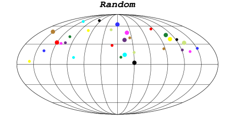
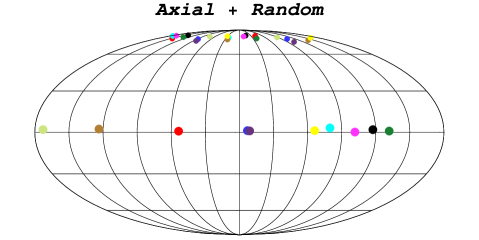
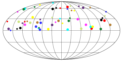
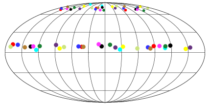
Figure 1: Mollweide projection of the sky with quadrupole (upper row) and octopole (lower row) multipole vectors [Equation (LABEL:eq_multp)]. The mesh consists of steps in $30^{\circ}$. Displayed are ten pairs of quadrupole vectors (small dots) and their ten area vectors [Equation (6) (big dots)] as well as ten triples of octopole vectors (small dots) and their area vectors (big dots); togetherness is indicated by color. The arbitrary sign of the vectors has been used to gauge them all to the northern hemisphere. The statistically isotropic and gaussian case (left column) is broken by the imprint of a strong axial effect $a_{\ell 0}=1000\mu$K (right column) whereupon multipole vectors move to the pole and area vectors move to the equatorial plane. The onset of the shown separation of multipole vectors and cross products can already be observed at moderate axial contributions of $a_{\ell 0}\sim 100\mu$K.

A common observable is the multipole power. According to the standard perception of inflationary cosmology, the CMB fluctuations are believed to follow a gaussian statistic and to be distributed in a statistically isotropic way. The notion of statistical isotropy means that the expectation value of pairs of coefficients $\langle a^{*}_{\ell^{\prime}m^{\prime}}a_{\ell m}\rangle$ is proportional to $\delta_{\ell^{\prime}\ell}\,\delta_{m^{\prime}m}$. Usually the proportionality constant measuring the expectation value of the multipole on the full sky is estimated by

$$C_{\ell}\equiv\frac{1}{2\ell+1}\sum_{m=-\ell}^{\ell}|a_{\ell m}|^{2}=\frac{1}{2\ell+1}\int{\rm d}\Omega\;T^{2}_{\ell}(\theta,\varphi)\;,$$ (1)

with $T_{\ell}$ being the $\ell$-th multipole of the CMB temperature anisotropy. It can be expanded with the help of spherical harmonics as: $T_{\ell}=\sum_{m}a_{\ell m}Y_{\ell m}$. Note that, since we consider multipole moments that are real, the $a_{\ell m}$ must fulfill an additional condition: $a^{*}_{\ell m}=(-1)^{m}a_{\ell-m}$. Using the estimator (1) the angular two-point correlation function is given by

$$C(\theta)=\frac{1}{4\pi}\sum_{\ell=0}^{\infty}(2\ell+1)C_{\ell}P_{\ell}(\cos\theta)\;,$$ (2)

where the $P_{\ell}$ are the Legendre Polynomials of $\ell$-th order.

Besides of the multipole power itself, it is useful to introduce an all-sky quantity that embraces all scales. As inspired by the $S_{1/2}$ statistic, presented in spergel03 for measuring the lack of angular power at scales larger than $60^{\circ}$, we use here an analogous all-sky statistic copi06 :

$$S_{\rm full}\equiv\int_{-1}^{1}C^{2}(\theta)\,{\rm d(cos}\theta)\;.$$ (3)

This is a measure of the total power squared on the full-sky. In contrast to the $S_{1/2}$ statistic spergel03 the $S_{\rm full}$ statistic does not contain any a priori knowledge on the variation of the two point angular correlation (2) for angles $>60^{\circ}$. Here we are considering especially the large angular scales but we are not interested in the monopole and dipole and thus arrive at

$$S_{\rm full}^{\rm trunc}=\frac{1}{8\pi^{2}}\left(5C_{2}^{2}+7C_{3}^{2}\right)\;.$$ (4)

Of course all multipoles have to be considered for the full-sky statistic (3) but we use the truncated part (4), because here the anomalies are most pronounced and we want to check for the interplay of this part of the full-sky power statistic with the other (phase) anomalies within quadrupole and octopole. This part is then simply to be added to the rest of the sum of (squared) multipole power in (3), recovering the expression for the full-sky.

Next we turn to the statistics involving the phase relationships of multipoles. We use the concept of Maxwell’s multipole vectors maxwell in order to probe statistical isotropy, since this representation proved to be useful for analyses of geometric alignments and special directions on the CMB sky. Normally the CMB data is decomposed into spherical harmonics and the coefficients $a_{\ell m}$ containing the physics. Alternatively, with the use of the multipole vectors formalism copi04 we can expand any real temperature multipole function on a sphere into

$$T_{\ell}(\theta,\varphi) = \sum_{m=-\ell}^{\ell}a_{\ell m}Y_{\ell m}(\theta,\varphi)$$

$$= A^{(\ell)}\left[\,\prod_{i=1}^{\ell}\left(\hat{\bm{v}}^{(\ell,i)}\cdot\hat{\bm{e}}(\theta,\varphi)\right)-\mathcal{L}_{\ell}(\theta,\varphi)\,\right]\;.$$

Therein $\hat{\bm{v}}^{(\ell,i)}$ is the $i$-th vector belonging to the multipole $\ell$ and $\hat{\bm{e}}(\theta,\varphi)=(\sin\theta\cos\varphi,\sin\theta\sin\varphi,\cos\theta)$ stands for a radial unit vector. With this decomposition all of the information in a multipole moment is reorganized such that we obtain a unique factorisation into a scalar $A^{(\ell)}$ counting the total power and $\ell$ unit vectors $\hat{\bm{v}}^{(\ell,i)}$ encoding all the directional information. The product expansion term alone contains also terms with ‘angular momentum’ $\ell-2,\ell-4,...$ These residuals are subtracted with the help of the term $\mathcal{L}_{\ell}(\theta,\varphi)$. Because all the signs of the multipole vectors may be absorbed in the scalar quantity $A^{(\ell)}$ the multipole vectors are unique up to their sign which carries no physical meaning. For definiteness, we define them to point to the northern hemisphere.

In order to disclose correlations among the multipole vectors we first consider for each $\ell$ the $\ell(\ell-1)/2$ independent oriented areas built from the cross products schwarz04 ; copi05 ; copi06 :

$${\bm{w}}^{(\ell;i,j)}\equiv\pm\;\hat{{\bm{v}}}^{(\ell,i)}\times\hat{{\bm{v}}}^{(\ell,j)}\;,$$ (6)

whereof we will also use the normalized vectors ${\bm{n}}^{(\ell;i,j)}\equiv{\bm{w}}^{(\ell;i,j)}/|{\bm{w}}^{(\ell;i,j)}|$. Now, in schwarz04 and subsequent works the dot products of the area vectors proved to be a handy expression in order to quantify alignments of the multipole vectors among each other and also with external directions (which we do not consider here). The following measure as stated in weeks and used in schwarz04 ; copi05 ; copi06 serves as a natural choice of a statistic in order to quantify the intrinsic alignment of quadrupole and octopole oriented areas:

$$S_{{\bm{w}}{\bm{w}}}\;\equiv\;\frac{1}{3}\,\sum_{i<j}\left|{\bm{w}}^{(2;1,2)}\cdot{\bm{w}}^{(3;i,j)}\right|\,.$$ (7)

Note that we consider only the very largest scales, i.e. we use the statistic only for $\ell=2,3$. Analogously, a statistic involving the normalized area vectors is given by:

$$S_{{\bm{n}}{\bm{n}}}\;\equiv\;\frac{1}{3}\,\sum_{i<j}\left|{\bm{n}}^{(2;1,2)}\cdot{\bm{n}}^{(3;i,j)}\right|\,.$$ (8)

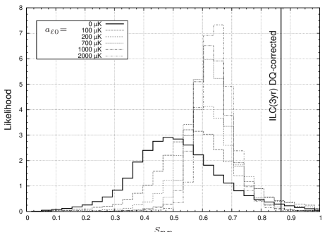
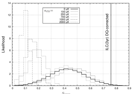
Figure 2: Evolution of the Monte Carlo likelihood of the alignment statistics $S_{{\bm{n}}{\bm{n}}}$ (7) and $S_{{\bm{w}}{\bm{w}}}$ (8). The effect of an axis in the CMB is modeled via increasing additional zonal harmonics with coefficients $a_{\ell 0}$. At $a_{\ell 0}=1000\mu$K the multipoles become purely zonal in good approximation. Regarding WMAP’s ILC(3yr) map $S_{{\bm{n}}{\bm{n}}}$ is unexpected at $98.3\%$C.L. and $S_{{\bm{w}}{\bm{w}}}$ is odd at $99.5\%$C.L. with respect to the statistically isotropic and gaussian sky (bold histograms). The best improvement is reached for both statistics at roughly $a_{\ell 0}=100\mu$K.

III Inflationary ${\bf\Lambda}$CDM predictions

Standard inflationary $\Lambda$CDM cosmology requires the CMB anisotropies to be gaussian and statistically isotropic. For the subsequent analysis we have produced Monte Carlo realisations of the harmonic coefficients $a_{\ell m}$ following the underlying $\Lambda$CDM theory. From copi04 an algorithm is available which we use to obtain Monte Carlo multipole vectors from the coefficients. Mollweide maps of a sample of random gaussian and statistically isotropic quadrupole and octopole vectors as well as their normals are given in Figure 1 (left column).

Concerning the question of correlations between the multipole power and the alignment of multipole vectors, it appears natural to expect that there is none. That is because we invoked gaussian random and statistically isotropic skies leading to multipole vectors (LABEL:eq_multp) independent of the multipole power (1). This assumption needs to be tested and quantified.

Nevertheless, a small correlation could be expected from the following reason: Considering only multipoles up to some limiting power, the resulting probability density distribution for the $a_{\ell m}$ must be non-gaussian. In fact, this restriction leads to a negative kurtosis for the $a_{\ell m}$ distribution (the skewness vanishes). Having that in mind, it appears suddenly unclear whether the naive expectation of vanishing correlation of power with intrinsic alignment will hold. Below we substantiate the absence of correlations by means of a Monte Carlo analysis.

Let us first look at the alignment anomalies. In Figure 2 the likelihood of the quadrupole and octopole alignment statistics $S_{{\bm{w}}{\bm{w}}}$ and $S_{{\bm{n}}{\bm{n}}}$ is shown. The predictions of the standard inflationary $\Lambda$CDM model are shown as the bold histograms respectively ($=$ vanishing axial contamination). According to the three-year ILC map from WMAP lambda we get the following measured values for the alignment statistics:

$$S_{{\bm{n}}{\bm{n}}}^{\rm ILC(3yr)}=0.8682\;\;\;\;\;\;,\;\;\;\;\;\;S_{{\bm{w}}{\bm{w}}}^{\rm ILC(3yr)}=0.7604$$

when copi06 corrected for the Doppler-quadrupole. The total number of Monte Carlos we produced per sample is $N=10^{5}$. We infer that the unmodified inflationary $\Lambda$CDM prediction is unexpected at $98.3\%$ C.L. with the $S_{{\bm{n}}{\bm{n}}}$ statistic and unexpected at $99.5\%$ C.L.  with respect to the $S_{{\bm{w}}{\bm{w}}}$ statistic.

Next we consider the cross-correlation between the intrinsic phase anomalies and the multipole power (1) within the low-$\ell$. For this we chose those $a_{\ell m}$ that allow for say the lowest possible $5\%$ in the left tail of the distributions for $C_{2}$ and $C_{3}$ that follow from statistical isotropy, gaussianity and the $\Lambda$CDM best-fit to the WMAP data. Then we compute the expression $S_{{\bm{w}}{\bm{w}}}$ for the selected $a_{\ell m}$ and compare it to the according ILC(3yr) value. As expected, no correlation is found, that is neither the shape nor the expectation value of the alignment statistic is shifted. We find the same also for the combination of the lowest allowed $5\%$ in $C_{2}$ and the highest $5\%$ from the right tail of the distribution of $C_{3}$ and the remaining two possible combinations thereof. As we do not find any correlations, we can conclude that the $S_{{\bm{w}}{\bm{w}}}$ and $S_{{\bm{n}}{\bm{n}}}$ statistics are not sensitive to the non-gaussianity induced by the restriction to low multipole power.

Moreover, we probe the opposite direction by tagging those $a_{\ell m}$ that lie in the allowed right tail of the $S_{{\bm{w}}{\bm{w}}}$ distribution with respect to $S_{{\bm{w}}{\bm{w}}}^{\rm ILC(3yr)}$. The distribution of the multipole power for $C_{2}$ and $C_{3}$ made of these $a_{\ell m}$ remains unchanged. The latter finding confirms that multipole power and the shape of multipoles (phases) are uncorrelated.

Using Equation (4), the lambda Maximum Likelihood Estimate (MLE) from the WMAP ILC(3yr) map for the angular power spectrum yields $S_{\rm full}^{\rm trunc,MLE}=29431\mu{\rm K}^{4}$. Compared to the value of $136670\mu{\rm K}^{4}$ from the $\Lambda$CDM best-fit to WMAP(3yr) data, this is not significantly unexpected, with an exclusion level of only $92.1\%$ C.L.

Now we want to check for correlations between the all-sky multipole power and the multipole alignment. As for reasons explained in the next section we prefer the $S_{{\bm{w}}{\bm{w}}}$ statistic to $S_{{\bm{n}}{\bm{n}}}$ in the following correlation analysis. In Figure 3 the scatter plot of $S_{{\bm{w}}{\bm{w}}}$ against $S_{\rm full}^{\rm trunc}$ is shown. The form of the contour can be understood as just the folding of the $\chi^{2}$-like form of the distribution for $S_{\rm full}^{\rm trunc}$ with the gaussian-like form of the $S_{{\bm{w}}{\bm{w}}}$ distribution. At first glance we see from Figure 3 that the MLE from WMAP(3yr) $S_{\rm full}^{\rm trunc,MLE}=29431\mu$K⁴ requires the alignment statistic to be of middle values (around $0.4$), which is inconsistent with the respective measured anomalous value from ILC(3yr). Moreover the lack of any linear behaviour in the contour suggests that there is no correlation between the two statistics.

sample size $N$	joint $p$	error $\Delta$
100000	$0.048\%$	$0.008\%$
100000	$0.001\%$	$0.002\%$
10000	$0.02\%$	$0.02\%$
1000	$0\%$	$0.02\%$

Table 1: Joint likelihoods (9) for $S_{\rm full}^{\rm trunc}$ and $S_{{\bm{w}}{\bm{w}}}$ being in accordance with data simultaneously. The experimental values refer to WMAP’s ILC(3yr) map lambda except for the second row. The error $\Delta$ of the factorisation in equation (9) is the difference between left hand side and right hand side in that equation.

Given that no correlation is present between $S_{{\bm{w}}{\bm{w}}}$ and $S_{\rm full}^{\rm trunc}$, we would expect that the joint probability that both power and alignment are in accordance with data factorizes according to:

$$p\left(S_{\rm full}^{\rm trunc}\leq{\rm data}\,\wedge\,S_{{\bm{w}}{\bm{w}}}\geq{\rm data}\right)=\hskip 72.26999pt$$

$$p_{1}\left(S_{\rm full}^{\rm trunc}\leq{\rm data}\right)\;p_{2}\left(S_{{\bm{w}}{\bm{w}}}\geq{\rm data}\right)\,.$$ (9)

But in reality we can only access finite statistical samples of these quantities and the factorisation will not be exact. However we will check the validity of (9) within our statistical ensemble. When using the full sample with $N=10^{5}$ respectively we obtain a joint likelihood of $p\simeq 0.05\%$. The error $\Delta$ of the factorisation, which we define as the difference between the left hand side in (9) and the right hand side, is of the order $\mathcal{O}(10^{-5})$, that is of the order of the Monte Carlo noise. In order to track the evolution of the error $\Delta$ we also compute the joint likelihood (9) for smaller subsamples; see Table 1. Reducing $N$ to $N=10^{4}$ we obtain an even smaller joint likelihood of $p=0.02\%$ but with an error that is of the same magnitude. With $N=10^{3}$ we do not have a single hit for the joint Monte Carlos leading to $p=0\%$ with the same error as in the $N=10^{4}$ case of $\Delta=0.02\%$. Note that just one Monte Carlo hit in favor of the joint case would raise the error here to $\Delta=0.08\%$. In the end, the convergence of the joint likelihood appears to be very slow with respect to the sample size $N$.

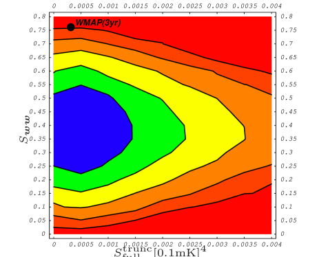
Figure 3: Contour of the scatter of intrinsic alignment (7) versus full-sky power squared (4). The shape can be understood from the folding of the two respective distributions. The total number of Monte Carlo points is $N=10^{5}$. The measured data point from WMAP three-year data is included. The maximum of likelihood requires $S_{{\bm{w}}{\bm{w}}}$ far smaller than obtained from ILC(3yr). Consistency with the data can be excluded at $99.95\%$ C.L. Contours correspond to lines of $1/2^{n}$ times the maximal likelihood, with $n=1,\dots,5$.

Furthermore we are interested in the stability of the results for $\Delta$ with respect to changes in the measured data. For this we choose the WMAP(1yr) values: $S_{\rm full}^{{\rm trunc,pseudo\text{-}}C_{\ell}}=10154\mu$K⁴ and $S_{{\bm{w}}{\bm{w}}}^{\rm ILC(1yr)}=0.7731$. We use a sample of the full size $N=10^{5}$ and obtain a joint likelihood with respect to the one-year data of $p=0.001\%$ with an error $\Delta=0.002\%$. That is, with respect to one-year data both the joint likelihood and its error are of the order of the Monte Carlo noise. From the WMAP(1yr) data alone we could exclude the joint case (9) rather conservatively at $99.99\%$ C.L. This appears to be a stronger exclusion than the one from three-year data. But we do not bother much about the difference because of the different estimators that have been used by the WMAP team for the angular power spectrum (pseudo-$C_{\ell}$ vs. MLE) lambda .

We quote the most conservative result, namely the full sample joint likelihood case for $S_{{\bm{w}}{\bm{w}}}$ and $S_{\rm full}^{\rm trunc}$ with respect to the WMAP(3yr) data. Therefore we can exclude that case at $>99.95\%$ C.L. with an error in the third digit after the comma lying within the Monte Carlo error of the used sample ($N=10^{5}$).

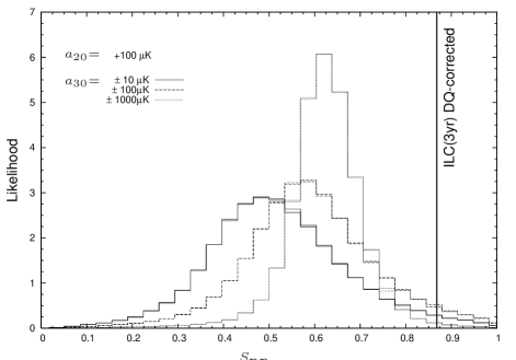
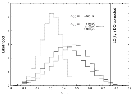
Figure 4: The sign of additional axial contributions $a_{\ell 0}$ has no physical effect on the statistics $S_{{\bm{n}}{\bm{n}}}$ and $S_{{\bm{w}}{\bm{w}}}$ . For the quadrupole this follows from the symmetry of the Legendre Polynomial $P_{2}$ [see Equation (12)]. The quadrupole contribution is kept fixed at $a_{20}=100\mu$K while the axial contribution to the octopole is varied both in magnitude and in sign. Respective pairs of $\pm a_{30}$ histograms lie virtually on each other and their statistics are thus indistinguishable. The reference histograms following from the axially unmodified $\Lambda$CDM model (bold histograms in Figure 2) lie nearly on top of the displayed $a_{20}=100\mu$K and $a_{30}=\pm 10\mu$K cases, and are thus not shown.

Finally we analyze the correlation of the all-sky power statistic $S_{\rm full}^{\rm trunc}$ and the intrinsic multipole alignment $S_{{\bm{w}}{\bm{w}}}$ by quantitative means:

It is well known from statistics, that when checking a finite two-dimensional sample for correlations, the empiric covariance

$${\rm cov}[\,S_{\rm full}^{\rm trunc}\,,\,S_{{\bm{w}}{\bm{w}}}\,]\equiv\hskip 130.08621pt$$

$$\frac{1}{N-1}\sum_{i=1}^{N}\left(S_{\rm full,\,i}^{\rm trunc}-\bar{S}_{\rm full}^{\rm trunc}\right)\left(S_{{\bm{w}}{\bm{w}},\,i}-\bar{S}_{{\bm{w}}{\bm{w}}}\right)$$ (10)

is a crucial quantity. The bar stands for the mean of a variable. As the covariance is a scale dependent measure, i.e. depending on the magnitudes of the sample values $S_{{\bm{w}}{\bm{w}},\,i}$ and $S_{{\bm{w}}{\bm{w}},\,i}$, the dimensionless Bravais-Pearson coefficient or empirical correlation coefficient is the better expression to use:

$$\rho_{S_{\rm full}^{\rm trunc}\,,\,S_{{\bm{w}}{\bm{w}}}}\equiv\frac{\rm cov[\,S_{\rm full}^{\rm trunc}\,,\,S_{{\bm{w}}{\bm{w}}}\,]}{\sqrt{{\rm cov}[\,S_{\rm full}^{\rm trunc}\,,\,S_{\rm full}^{\rm trunc}\,]\,{\rm cov}[\,S_{{\bm{w}}{\bm{w}}}\,,\,S_{{\bm{w}}{\bm{w}}}}\,]}\;.$$

Finally, employing the WMAP(3yr) data we obtain an empirical correlation coefficient of $\rho_{S_{\rm full}^{\rm trunc},S_{{\bm{w}}{\bm{w}}}}=-0.0027$ with respect to the full sample $N=10^{5}$, which indeed indicates only marginal correlation.

IV Inclusion of an Axis

Now we ask what happens when introducing axial contributions on top of a statistically isotropic and gaussian microwave sky. The presence of a preferred direction with axisymmetry in the CMB will exclusively excite the zonal modes in case the axis is collinear to the ${\bm{z}}$-axis. Here we do not bother about external directions since the internal alignments are independent of these. Therefore such an axis will manifest itself through additional contributions $a_{\ell 0}$. We are considering the quadrupole and the octopole and the question arises, in how far the sign of the axial contributions $\pm a_{\ell 0}$ plays a role. The coefficients $a_{\ell m}$ can be reconstructed from

$$a_{\ell m}=\int\frac{\Delta T}{T}(\theta,\varphi)\;Y_{\ell m}^{*}\;{\rm d}\Omega\;.$$ (12)

Obviously, within the quadrupole the sign of $\pm a_{20}$ is irrelevant because of the symmetry of the Legendre Polynomial $P_{2}$ with respect to $\theta=90^{\circ}$. The Legendre Polynomial $P_{3}$ however is antisymmetric with respect to $\theta=90^{\circ}$. Therefore the relevance of the sign of the octopole contributions $a_{30}$ has to be clarified. Consequently we have chosen a fixed value for the axial quadrupole contribution $a_{20}$ and have then varied the according octopole contribution in sign and in magnitude. The results are displayed in Figure 4. Apparently the $S_{{\bm{n}}{\bm{n}}}$ and $S_{{\bm{w}}{\bm{w}}}$ statistics that are important here, do not distinguish between the sign of the applied axial effect. Therefore we need not to bother about the signs of the $a_{\ell 0}$ and let them henceforth be positive.

In Figure 2 the evolution of the $S_{{\bm{w}}{\bm{w}}}$ and $S_{{\bm{n}}{\bm{n}}}$ statistics with respect to increasing axial contributions is displayed in terms of likelihood histograms:

Let us first look at the evolution of the $S_{{\bm{n}}{\bm{n}}}$ statistic. This expression measures the average $|\cos|$ of the angles between the quadrupole oriented area and the octopole areas. The pure Monte Carlo peaks at $0.5$ reflecting the fact that the average distance of four isotropically distributed vectors on a half–sphere from each other is $60^{\circ}$ in the case of statistical isotropy. It is a half-sphere because the signs of the multipole vectors are arbitrary and so we choose them all to point to the northern hemisphere. When increasing the contribution of the axial effect the multipoles become increasingly zonal and arrive at being purely zonal in a good approximation at values of $a_{\ell 0}=1000\mu$K. On the level of the multipole vectors this means that their cross products all move to the equatorial plane (see Figure 1). That is the reason why the histogram in Figure 2 (left) moves to the right when we increase the axial effect, because now isotropy is broken from the half-sphere to the half-circle making the $S_{{\bm{n}}{\bm{n}}}$ histogram peak sharper at higher values. The measured value from the ILC(3yr) map of $S_{{\bm{n}}{\bm{n}}}^{\rm ILC(3yr)}=0.868$ is anomalous at $98.3\%$ C.L. with respect to the pure Monte Carlo (bold histogram in Figure 2) which stands for the statistically isotropic and gaussian model. By adding axial contribution the maximal improvement is reached at $a_{\ell 0}=100\mu$K where the ILC(3yr) becomes unexpected at $96.7\%$ C.L. Further enhancement of the axial effect makes the $S_{{\bm{n}}{\bm{n}}}$ statistic more and more narrow around an expectation value $<0.7$. This makes it impossible to remove the anomaly in the $S_{{\bm{n}}{\bm{n}}}$ cross-alignment with respect to the ILC(3yr) experimental value only by increasing the axial contribution to high enough values.

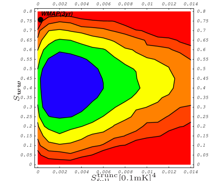
Figure 5: Scatter contour of pairs of $S_{{\bm{w}}{\bm{w}}}$ and $S_{\rm full}^{\rm trunc}$ after an axial modification of $a_{\ell 0}=70\mu$K has been applied; this is the contribution involving maximal improvement in $S_{{\bm{w}}{\bm{w}}}$ (see Figure 2). The total number of Monte Carlo pairs is $N=10^{5}$. Note that the horizontal axis now runs from zero to $1.4\times 10^{-6}{\rm mK}^{4}$, whereas in Figure 3 the maximal displayed value is $4\times 10^{-7}{\rm mK}^{4}$. The inclusion of a preferred axis leaves all-sky multipole power and intrinsic alignment totally uncorrelated and inconsistent with the WMAP(3yr) data. Contour lines are defined as in Figure 3.

On the other hand the $S_{{\bm{w}}{\bm{w}}}$ statistic additionally measures the modulus of the sin of the angles between the multipole vectors themselves. As can be seen from Figure 1 multipole vectors are all moving toward the north pole clustering more and more as the axial contribution is enhanced. The $S_{{\bm{w}}{\bm{w}}}$ statistic measures the average of the modulus of the products of the sin of angles between quadrupole vectors, octopole vectors and the cos of the angle between the area vectors. Therefore on top of the information already contained in $S_{{\bm{n}}{\bm{n}}}$ the $S_{{\bm{w}}{\bm{w}}}$ statistic is able to go to zero for highest zonal contamination as the closeness of the multipole vectors in that case dampens the product of sines and cosines quadratically to arbitrary small values. Thus we find that $S_{{\bm{w}}{\bm{w}}}$ is the more convenient statistic for further analyses, as it does contain more information than the $S_{{\bm{n}}{\bm{n}}}$ statistic and additionally shows a simple and clear asymptotic behavior. In the case of this statistic the anomaly is significant at $99.5\%$C.L. with respect to $S_{{\bm{w}}{\bm{w}}}^{\rm ILC(3yr)}=0.7604$. Similarly to before the maximal improvement is reached with an axial contribution of $a_{\ell 0}=70\mu$K, which degrades the anomaly in $S_{{\bm{w}}{\bm{w}}}$ to $99.2\%$C.L.

Now we return to the correlation analysis of the alignment with the pure multipole power $C_{\ell}$. When introducing an axial effect, say $a_{\ell 0}=100\mu$K, we improve the fit to the $S_{{\bm{w}}{\bm{w}}}$ statistic, but interestingly the multipole power anomaly becomes much more pronounced. This behaviour is expected rse1 ; rse2 for the $C_{\ell}$-distribution (being a modified $\chi^{2}$-distribution) when the axial contribution is enhanced, but it is unexpected that exactly the same happens for a multipole power distribution ‘that knows of the intrinsic alignment of quadrupole and octopole’. This indicates that there is no correlation at all between multipole power and the phase alignment even when they are tuned to each other.

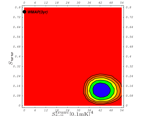
Figure 6: Contour plot of the scatter of pairs $(S_{{\bm{w}}{\bm{w}}},S_{\rm full}^{\rm trunc})$ after a strong axial contingent of $a_{\ell 0}=1000\mu$K is induced to the multipole vectors (see also Figures 1,2). The total number of Monte Carlo pairs is $N=10^{5}$. The all-sky power statistic reacts heavily as the scale on the $S_{\rm full}^{\rm trunc}$-axis is shifted by four orders of magnitude with respect to the case of $a_{\ell 0}=70\mu$K (Figure 5). The likelihood maximum departs very articulately from the WMAP(3yr) data. The contour lines are defined like in Figure 3.

Proceeding with the analysis of correlations between alignment and the full-sky power statistic, again we try to provoke correlation with the help of axial symmetry in the CMB. In fact we apply an axial effect of the ideal magnitude ($a_{\ell 0}=70\mu$K) in order achieve larger values in $S_{{\bm{w}}{\bm{w}}}$. The negative result is shown in Figure 5: As $S_{\rm full}^{\rm trunc}$ is a linear combination of squared $C_{\ell}$ distributions it is a sharply peaked $\chi^{2}$-like distribution being very sensitive to axial contributions. Therefore the contour in Figure 6 is fairly shifted to the right (to higher values in $S_{\rm full}^{\rm trunc}$) and broadened with respect to the axially unmodified case, obviating any correlation with the intrinsic alignment. The shape of the overall contour is roughly left invariant by the scale shift in $S_{\rm full}^{\rm trunc}$.

Figure 6 illustrates the pure zonal case. Here a whole $a_{\ell 0}=1000\mu$K has been induced into the multipole vectors. Again, due to the sensitivity of $S_{\rm full}^{\rm trunc}$ to axial contamination this pushes the allowed region in the scatter plot to very high values in full-sky power squared, degenerating the contour to a ‘small’ area far away from the measured three-year WMAP values. No change in correlation is observable.

Obviously, no coupling of the multipole power statistic and the intrinsic alignment can be driven in favor of the anomalous experimental CMB data by an additional axisymmetric effect on top of the primordial fluctuations.

V Conclusions

We have shown that a literal interpretation of the ‘Axis of Evil’ as an axisymmetric effect is highly incompatible with the observed microwave sky at the largest angular scales. The formalism of multipole vectors was used to separate directional information from the absolute power of multipoles on the CMB sky. Considered were two choices of statistic, measuring the intrinsic cross-alignment between the quadrupole and octopole: the $S_{{\bm{n}}{\bm{n}}}$ and the $S_{{\bm{w}}{\bm{w}}}$ statistic. We confirm that the $S_{{\bm{w}}{\bm{w}}}$ statistic contains more information on the multipoles and that it has more discriminative power as an axial effect is included. The presence of an axial symmetry in the CMB would excite zonal modes which are, in the frame of the axis, additional $a_{\ell 0}$ contributions in the language of the harmonic decomposition. Both statistics ($S_{{\bm{n}}{\bm{n}}}$ and $S_{{\bm{w}}{\bm{w}}}$) reach slightly better agreement with the measured values from the ILC(3yr) map at amplitudes of roughly $a_{\ell 0}=100\mu$K. Further enhancement of the axial effect only reduces consistency with WMAP(3yr) data.

Especially we have assayed in what way the alignment anomaly between quadrupole and octopole can affect the respective multipole power. We made several tests where we identified and selected the ‘anomalous $a_{\ell m}$’ that are still consistent with data and checked whether the resulting distribution from these $a_{\ell m}$ for either power or alignment shows any change with respect to the unbiased case. For the all-sky multipole power we make use of the statistic $S_{\rm full}^{\rm trunc}$. We demonstrated that the correlation between $S_{\rm full}^{\rm trunc}$ and intrinsic alignment is only marginal (correlation coefficient of $-0.0027$). Thus a factorisation of the probability for the joint case into a product of the respective probabilities is allowed.

We argued that the combined case of the measured all-sky power and the quadrupole-octopole alignment is anomalous at $>99.95\%$ C.L. with respect to the WMAP three-year data. The correlation picture leaves no space for an axisymmetric effect in the large-angle CMB.

These findings complement our previous studies rse1 of the interplay of an axisymmetric effect and the extrinsic CMB anomalies (correlation with the motion and orientation of the Solar system schwarz04 ). In that work it was shown that an axisymmetric effect might help to explain a Solar system alignement. Finally, this study rules out that possibility.

But there is a loophole. Here and in rse1 we only considered additive modifications of the $a_{\ell m}$. Still, a preferred axis could also induce multiplicative modifications in all $a_{\ell m}$ huhu06 . This could avoid the problem of additional multipole power. However, multiplicative effects could only be achieved by non-linear physics, like systematics of the measurement or the map making process.

A modelling that would be able to consistently remove both the power and the intrinsic alignment problem for low-$\ell$ must mobilize a more complex pattern of modifications than the one induced by an axisymmetric effect. As already indicated by e.g. the odd extrinsic alignment with the ecliptic schwarz04 ; copi05 ; copi06 ; rse1 ; rse2 the CMB anomalies do rather require a special plane than a preferred axis. The so called ‘Axis of Evil’ appears as just the normal vector of that plane, but no axial symmetry is present within that plane.