Superfluid neutron star turbulence

Abstract

We analyse the implications of superfluid turbulence for neutron star physics. We begin by extending our previous results for the mutual friction force for a straight vortex array to account for the self-induced flow which arises when the vortices are curved. We then discuss Vinen’s phenomenological model for isotropic turbulence, and derive the associated (Gorter-Mellink) form for the mutual friction. We compare this derivation to a more recent analysis of Schwarz, which sheds light on various involved issues. Having discussed isotropic turbulence, we argue that this case is unlikely to be relevant for neutron stars. Instead we expect a rotating neutron star to exhibit polarised turbulence, where relative flow drives the turbulence and rotation counteracts it. Based on recent results for superfluid Helium, we construct a phenomenological model that should have the key features of such a polarised turbulent system.

1 Introduction

Turbulence in superfluid Helium has been exciting experimenters and theorists in low temperature physics for the last 50 years. Not surprisingly, the literature on the subject is vast, and the research has reached the level where theoretical models represent experimental data relatively well (Donnelly, 1991). Meanwhile, the possibility that turbulence may be relevant for neutron star superfluidity has hardly been discussed at all (although see the recent work by Peralta et al (2005, 2006)). This is quite surprising because the standard models for neutron stars are strongly inspired by the two-fluid model for superfluid Helium. There may be differences between the two problems, but the underlying multifluid dynamics is essentially the same (Mendell, 1991a; Prix, 2004; Andersson & Comer, 2006). One would expect this to be particularly true for the vortex dynamics and the processes that lead to vortex tangles and turbulent behaviour.

The aim of this paper is to discuss turbulence in superfluid neutron stars. In particular, we want to extend the description of the mutual friction force (Alpar, Langer & Sauls, 1984; Mendell, 1991b; Andersson, Sidery & Comer, 2006), that couples the two components in a superfluid neutron star core, in such a way that we can account for vortex tangles. This is an important first step along a road that should eventually lead to an improved description of superfluid neutron star dynamics. The mutual friction coupling enters in the analysis of three important astrophysics problems. First of all, it sets the timescale on which the two core fluids are coupled following a pulsar glitch (or any event that involves a velocity difference) (Alpar & Sauls, 1988; Jahan Miri, 1998; Andersson, Sidery & Comer, 2006). Secondly, it is one of the key mechanisms that determine the damping rate of neutron star free precession (Jones & Andersson, 2001). Finally, the mutual friction is one of the main damping agents for superfluid neutron star oscillations. In particular, it has been argued that the mutual friction damping completely suppresses the gravitational-wave driven instability of the fundamental f-modes (Lindblom & Mendell, 1995). It is also one of the key damping mechanisms affecting the analogous instability of the inertial r-modes (Lindblom & Mendell, 2000), see Andersson (2003) for a review. However, all existing results have been obtained by making use of the form of the mutual friction first suggested by Hall & Vinen (1956) for Helium. Since this model is based on the assumption on a straight vortex array it is not relevant when the vortices form a disorganised tangle. The mutual friction force that applies in this case is known to be rather different (Vinen, 1957). This suggests that, if neutron stars exhibit turbulent behaviour, then much of the generally accepted thinking about the interior superfluid dynamics may be wrong.

2 The straight vortex case

We have recently discussed the mutual friction force, and the associated coefficients, that should apply when the vortices are straight (Andersson, Sidery & Comer, 2006). This should be the relevant case for uniformly rotating systems, provided that the vortex array is dynamically stable (which may not be the case). Our analysis was based on the standard two-fluid model (Prix, 2004; Andersson & Comer, 2006) where the superfluid neutrons, with mass density $\rho_{\rm n}$ and velocity $v^{i}_{\rm n}$, are distinguished from a conglomerate of all charged components, represented by $\rho_{\rm p}$ and $v^{i}_{\rm p}$ and loosely refered to as the “protons”. In absence of dissipation the equations of motion for the two fluids can be written

$$\left(\frac{\partial{}}{\partial{t}}+{v}^{j}_{{\mathrm{x}}}\nabla_{j}\right)\left[{v}_{i}^{{\mathrm{x}}}+\varepsilon_{{\mathrm{x}}}w_{i}^{{\mathrm{y}}{\mathrm{x}}}\right]+\nabla_{i}(\Phi+\tilde{\mu}_{{\mathrm{x}}})+\varepsilon_{{\mathrm{x}}}w_{j}^{{\mathrm{y}}{\mathrm{x}}}\nabla_{i}v^{j}_{{\mathrm{x}}}=0\ .$$ (1)

where the contituent indices ${\mathrm{x}}$ and ${\mathrm{y}}\neq{\mathrm{x}}$ can be either ${\rm n}$ or ${\rm p}$. The relative velocity is defined as

$$w_{i}^{{\mathrm{y}}{\mathrm{x}}}={v}_{i}^{{\mathrm{y}}}-{v}_{i}^{{\mathrm{x}}}\ .$$ (2)

Furthermore,

$$\tilde{\mu}_{\mathrm{x}}={\mu_{\mathrm{x}}\over m_{\mathrm{x}}}={1\over m_{\mathrm{x}}}{\partial E\over\partial n_{\mathrm{x}}}\ ,$$ (3)

where $E$ is an energy functional (which represents the equation of state in this formalism) and $\tilde{\mu}_{\mathrm{x}}$ is the relevant chemical potential per unit mass. The coefficients

$$\varepsilon_{\mathrm{x}}={2\alpha\over\rho_{\mathrm{x}}}\qquad\mbox{ where }\qquad\alpha={\partial E\over\partial w_{{\rm n}{\rm p}}^{2}}\ ,$$ (4)

encode what is known as the entrainment effect, and $\Phi$ represents the gravitational potential. For a detailed discussion of these equations, see Prix (2004) and Andersson & Comer (2006). Since the equations of motion represent momentum balance, we see that the momentum per fluid element is

$$p_{i}^{\mathrm{x}}=m_{\mathrm{x}}[{v}_{i}^{{\mathrm{x}}}+\varepsilon_{{\mathrm{x}}}w_{i}^{{\mathrm{y}}{\mathrm{x}}}]\ ,$$ (5)

This illustrates the main impact of the entrainment. The momentum of the each fluid need not be parallel with that fluids transport velocity. This effect is important for neutron star cores because the strong force endowes each neutron with a cloud of protons (and vice versa). This affects the effective mass of the particle and, when it moves, alters the momentum. As discussed by, for example, Andersson, Sidery & Comer (2006) the entrainment can be related to the effective proton mass $m_{\rm p}^{*}$ via

$$2\alpha=\rho_{\rm p}\varepsilon_{\rm p}=n_{\rm p}(m_{\rm p}-m_{\rm p}^{*})=n_{\rm p}\delta m_{\rm p}^{*}\ .$$ (6)

Formally, the above equations represent a macroscopic average over a large number of individual fluid elements (in the standard way). This is a natural approach for neutron stars where one is interested in fluid dynamics at lengthscales vastly larger than the inter-particle separation. However, in order to assign values to the various parameters (like the entrainment $\alpha$) one must regularly resolve the problem at the microscopic level. This then raises issues concerning the averaging procedure which is required to make contact with the macroscopic level. In problems involving vortex dynamics, the situation is made even more complex. It is then natural to introduce an intermediate “mesoscopic” level which is sufficiently large that one can average over a large collection of particles (and hence discuss “fluid” dynamics in a sensible way) and yet small enough that one can resolve the individual vortices. The macroscopic equations then derive from an averaging over a large set of vortices, leading to the smooth equations of motion (1). As we will see, this averaging is one of the key problems that must be overcome in a description of superfluid turbulence.

On the mesoscopic level, the motion of a neutron vortex is affected by fluid flow past it (via the Magnus “force”). At the same time, the circulation associated with the vortex induces circular flow in the protons because of the entrainment. This in turn generates a magnetic field on the vortex, and the scattering of electrons off of this field acts resistively on the vortex motion (Alpar, Langer & Sauls, 1984). Taking this resistive force to be proportional to the difference in velocity between the vortex ($v_{\rm L}^{i}$) and the charged fluid flow we have

$$f_{i}^{\mathrm{e}}={\cal R}(v^{{\rm p}}_{i}-v^{{\rm L}}_{i})\ .$$ (7)

acting per unit length of the vortex. Neglecting the inertia of the vortex core, and balancing $f_{i}^{\mathrm{e}}$ to the Magnus “force” we arrive at the mutual friction acting on the neutrons (per unit length of vortex)

$$f^{\rm mf}_{i}={\cal B}^{\prime}\rho_{\rm n}\epsilon_{ijk}\kappa^{j}w_{{\rm n}{\rm p}}^{k}+{\cal B}\rho_{\rm n}\epsilon_{ijk}\epsilon^{klm}\hat{\kappa}^{j}\kappa_{l}w^{{\rm n}{\rm p}}_{m}\ ,$$ (8)

(correcting an overall sign error resulting from Andersson, Sidery & Comer (2006) writing the consitutent indices in the wrong order). The same force acts on the vortex and an equal and opposite force affects the protons. The vector $\kappa^{i}$ determines the orientation of the vortex (see later) and its magnitude (the quantum of circulation) is $\kappa=h/2m_{\rm n}\approx 2\times 10^{-3}$ cm²/s. Our estimated (dimensionless) mutual friction coefficients are

$${\cal B}={{\cal R}\over\rho_{\rm n}\kappa}\approx 4\times 10^{-4}\left({\delta m_{\rm p}^{*}\over m_{\rm p}}\right)^{2}\left({m_{\rm p}\over m_{\rm p}^{*}}\right)^{1/2}\left({x_{\rm p}\over 0.05}\right)^{7/6}\left({\rho\over 10^{14}\mathrm{g/cm}^{3}}\right)^{1/6}\ ,$$ (9)

and

$${\cal B}^{\prime}={\cal B}^{2}\ ,$$ (10)

where $x_{\rm p}=\rho_{\rm p}/\rho$ is the proton fraction, in agreement with previous estimates by Alpar, Langer & Sauls (1984) and Mendell (1991b).

In order to complete the description of the mutual friction force we need to note that the equations of motion (1) are relevant on the macroscopic scale. Meanwhile the analysis leading to (8) is mesoscopic, as we are considering a single vortex. The macroscopic equations of motion follow if we average over a large collection of vortices, i.e. we need to work at a sufficiently large lengthscale that such averaging is meaningful. We also need to note that the Magnus effect is already accounted for in the left-hand side of (1), which means that we only need to add the smooth averaged form of the force (8) to the right-hand side. In the particular case of a straight vortex array, the required averaging is easy. To get the required force per unit volume we simply need to multiply (8) by the local number density of vortices per unit area, $n_{v}$.

As we will face this issue again later, it is useful to discuss it in a little bit more detail here. At the fluid dynamics level, we introduce the “rotation velocity” in the standard way,

$$2\Omega_{\mathrm{x}}^{i}=\epsilon^{ijk}\nabla_{j}v_{k}^{\mathrm{x}}\ ,$$ (11)

This means that, on the macroscopic level we identify (assuming that the lengthscale considered is sufficiently small that we can treat $\varepsilon_{\rm n}$ as constant)

$$\epsilon^{ijk}\nabla_{j}p^{\rm n}_{k}=2m_{\rm n}[\Omega_{\rm n}^{i}+\varepsilon_{\rm n}(\Omega_{\rm p}^{i}-\Omega_{\rm n}^{i})]\ .$$ (12)

Meanwhile, at the mesoscopic level the circulation of neutron momentum (not velocity) is quantised. Representing the mesoscopic “momentum” by $\bar{p}_{\rm n}^{k}$, we have

$${1\over m_{\rm n}}\epsilon_{ijk}\nabla^{j}\bar{p}_{\rm n}^{k}=\kappa_{i}={h\over 2m_{\rm n}}\hat{\kappa}_{i}\ .$$ (13)

Strictly speaking, we should arrive at the first equation by averaging the second. Denoting the average by angular brackets we have (in the case of straight vortices)

$$\langle\epsilon^{ijk}\nabla_{j}\bar{p}^{\rm n}_{k}\rangle=n_{v}m_{\rm n}\kappa^{i}=\epsilon^{ijk}\nabla_{j}p^{\rm n}_{k}$$ (14)

Hence we see that

$$n_{v}\kappa=2[\Omega_{\rm n}+\varepsilon_{\rm n}(\Omega_{\rm p}-\Omega_{\rm n})]\ .$$ (15)

3 Are superfluid neutron stars likely to be turbulent?

We want to extend our description of the mutual friction force to the more complicated situation where the vortices are curved and may reconnect to form a turbulent tangle. Before we try to do this, it is useful to have some guidance as to whether one would expect turbulence to be relevant for superfluid neutron stars. After all, virtually every discussion of neutron star vortex dynamics has made the assumption that the vortex array is straight. Should this basic tenet fall, a possibility that has been hinted at by, for example, Packard (1972) and Chevalier (1995), we might have to reassess much of our current “wisdom”.

To get an idea of the possible relevance of superfluid turbulence, let us adapt a recent argument due to Finne et al (2003). They consider the problem for superfluid ³He, and argue that an intrinsic parameter determines the onset of turbulence. In our case, the argument would proceed as follows. First assume that the motion of the “normal fluid” can be neglected, i.e. take $v_{i}^{\rm p}=0$. This is convenient becase we then do not have to worry about the effects of entrainment. In the Helium case it may also be quite reasonable because one can assume that the normal fluid is viscous and essentially immobile with respect to the walls of the container (at least on a timescale large compared to the viscous timescale), In our case, the equation of motion for the neutrons can then be written

$$(\partial_{t}+v_{\rm n}^{j}\nabla_{j})v_{i}^{\rm n}+\nabla_{i}[\ldots]={1\over\rho_{\rm n}}f^{\mathrm{mf}}_{i}$$ (16)

This is easily rewritten as

$$\partial_{t}v_{i}^{\rm n}+\nabla_{i}[\ldots]=\epsilon_{ijk}v_{\rm n}^{j}\omega_{\rm n}^{k}+{1\over\rho_{\rm n}}f^{\mathrm{mf}}_{i}$$ (17)

where $\omega_{\rm n}^{i}=\epsilon^{ijk}\nabla_{j}v^{\rm n}_{k}$, Taking the curl of this equation, and using (8), we arrive at (assuming that the various parameters are constant)

$$\partial_{t}\vec{\omega}^{\rm n}=(1-\mathcal{B}^{\prime})\nabla\times(\vec{v}_{\rm n}\times\vec{\omega}_{\rm n})+\mathcal{B}\nabla\times[\hat{\omega}_{\rm n}\times(\vec{\omega}_{\rm n}\times\vec{v}_{\rm n})]$$ (18)

Comparing to the standard fluid case, Finne et al (2003) argues that the first term on the right hand side (the inertial term) induces the transfer of energy to smaller length scales, i.e. drives the turbulence. Meanwhile, the second term leads to damping that serves to stabilise the flow. The relative importance of the two effects is determined by the parameter

$$q={\mathcal{B}\over 1-\mathcal{B}^{\prime}}$$ (19)

If $q<1$ one might expect the flow to become turbulent. This is in quite good agreement with the experimental evidence provided by Finne et al (2003). They show that turbulence sets in for $q\leq 1.3$ or so. Further quantitative evidence for this idea has been provided by Henderson & Barenghi (2004). They analyse the spectrum of Kelvin waves in the vortex array, and argue that $q=1$ represents the crossover point at which these waves change from being overdamped (damping out before completing a full oscillation) to propagating. The idea would be that the vortex oscillations can then lead to reconnections with neighbouring vortices. This is obviously more likely to happen if the waves propagate along the vortex array. Anyway, in the neutron star case we have already shown that $\mathcal{B}^{\prime}\approx\mathcal{B}^{2}\ll 1$. Hence, we would always have $q\ll 1$, and according to the above criterion one would expect a superfluid neutron star core to be extremely susceptible to becoming turbulent. Of course, there are a number of caveats. Most importantly, the argument does not account for the stabilising effect of rotation. Nevertheless, it is clear that we must take the possibility of superfluid turbulence seriously.

4 Accounting for vortex curvature

The mutual friction force (8) is only relevant when the vortices are straight. This should be the case in a star that is uniformly rotating, assuming that the vortex array is dynamically stable. This has generally been taken to be the case for neutron stars. However, work on the analogous problem for superfluid Helium indicates that there will exist a critical relative flow above which oscillations are induced in the vortices rendering the array unstable (Glaberson, Johnson & Ostermeier, 1974). This leads to the formation of a complex vortex tangle and a state of turbulence. As a first step towards understanding the implications of this for neutron stars we will generalise the mutual friction force to the case of isotropic turbulence. To do this, we need to move away from the assumption that the vortices are straight.

The induced flow due to the vortex curvature will play a key rôle in our discussion. The analysis of this problem for superfluid Helium (Donnelly, 1991) is easily extended to the neutron star case. This is not surprising since the basic nature of the rotational vortices is the same. Nevertheless, the derivation is provided in Appendix A. It should be useful for readers that are unfamiliar with the Helium results. Moreover, our analysis accounts for the entrainment effect which has (as far as we know) not been considered in previous work. Yet we know that it is important for neutron star dynamics. In fact, one would not be at all surprised if (at the end of the day) it were relevant for the Helium problem as well.

As demonstrated in Appendix A, the vortex curvature induces a contribution to the (mesoscopic) neutron momentum

$${\bar{p}^{\mathrm{ind}}_{i}\over m_{\rm n}}=\nu\epsilon_{ijk}s^{\prime j}s^{\prime\prime k}$$ (20)

where

$$\nu={\kappa\over 4\pi}\log\left({b\over a_{0}}\right)$$ (21)

and we also know that

$$s^{\prime}_{i} = \hat{\kappa}_{i}$$ (22)

$$s^{\prime\prime}_{i} = \hat{\kappa}^{j}\nabla_{j}\hat{\kappa}_{i}$$ (23)

To get an idea of the value of the parameter $\nu$, which determines the tension in the vortex array, we note that a typical value of the size of the vortex core would be $a_{0}\approx 100$ fm, while we can let $b$ be given by the inter-vortex spacing. This would mean that (for the usual triangular vortex configuration) we would have

$$b\approx 3.4\times 10^{-3}\left({\Omega_{\rm n}\over 100\mbox{ rad/s}}\right)^{-1/2}\mbox{ cm}$$ (24)

Combining these we see that

$$\log\left({b\over a_{0}}\right)\approx 20-{1\over 2}\log\left({\Omega_{\rm n}\over 100\mbox{ rad/s}}\right)$$ (25)

In other words, for superfluid rotation rates at the opposite ends of the range of observed pulsar periods, $P=10^{-3}-10$ s (say) the value of $\nu$ only varies by about 30%. It is also worth noting that $\nu$ is similar in the Helium case. Typical values would then be $a_{0}\approx 10^{-8}$ cm and $b\approx 10^{-2}$ cm, leading to $\log(b/a_{0})\approx 14$.

Having derived the curvature-induced momentum for a single vortex, we can apply the result to the two-fluid model for a neutron star core. As discussed by Andersson, Sidery & Comer (2006), the presence of a neutron vortex will affect the flow of both neutrons and protons. The induced flow makes a contribution

$${\bar{p}_{i}^{\rm n}\over m_{\rm n}} = v_{i}^{\rm n}+\varepsilon_{\rm n}(v_{i}^{\rm p}-v_{i}^{\rm n})={\bar{p}^{\mathrm{ind}}_{i}\over m_{\rm n}}$$ (26)

$${\bar{p}_{i}^{\rm p}\over m_{\rm p}} = v_{i}^{\rm p}+\varepsilon_{\rm p}(v_{i}^{\rm n}-v_{i}^{\rm p})=0$$ (27)

Solving these equations for the individual velocities, we find

$$v^{{\rm n}}_{i}=\frac{1-\varepsilon_{{\rm p}}}{1-\varepsilon_{{\rm n}}-\varepsilon_{{\rm p}}}\nu\epsilon_{ijk}s^{\prime j}s^{\prime\prime k}$$ (28)

$$v^{{\rm p}}_{i}=-\frac{\varepsilon_{{\rm p}}}{1-\varepsilon_{{\rm n}}-\varepsilon_{{\rm p}}}\nu\epsilon_{ijk}s^{\prime j}s^{\prime\prime k}$$ (29)

That is, the difference between the two induced velocities is

$$v^{{\rm n}}_{i}-v^{{\rm p}}_{i}=\tilde{\nu}\epsilon_{ijk}s^{\prime j}s^{\prime\prime k}$$ (30)

where we have defined

$$\tilde{\nu}=\frac{1}{1-\varepsilon_{{\rm n}}-\varepsilon_{{\rm p}}}\nu$$ (31)

How do these additional contributions to the flow affect the mutual friction force? The answer is quite intuitive. The induced velocities simply add to the general flows $v_{\mathrm{x}}^{i}$ in the expression for the force (8). Adding the velocity difference (30) to the overall relative velocity in (8), and noting that

$$\vec{s}^{\prime}\times(\vec{s}^{\prime}\times\vec{s}^{\prime\prime})=-\vec{s}^{\prime\prime}\ ,$$ (32)

we find that the additional contribution to the mutual friction force can be written

$$f^{\rm ind}_{i}=-\rho_{\rm n}\kappa\tilde{\nu}\left[{\cal B}^{\prime}s_{i}^{\prime\prime}+{\cal B}\epsilon_{ijk}s^{\prime j}s^{\prime\prime k}\right]\ ,$$ (33)

or equivalently

$$f^{\rm ind}_{i}=-\rho_{\rm n}\kappa\tilde{\nu}\left[{\cal B}^{\prime}\hat{\kappa}^{j}\nabla_{j}\hat{\kappa}_{i}+{\cal B}\epsilon_{ijk}\hat{\kappa}^{j}\hat{\kappa}^{l}\nabla_{l}\hat{\kappa}^{k}\right]$$ (34)

To get an expression for the total mutual friction force, these terms should be added to (8). Thus we get the force per unit length

$$f^{\rm mf}_{i}={\cal B}^{\prime}\rho_{\rm n}\epsilon_{ijk}\kappa^{j}w_{{\rm n}{\rm p}}^{k}+{\cal B}\rho_{\rm n}\epsilon_{ijk}\epsilon^{klm}\hat{\kappa}^{j}\kappa_{l}w^{{\rm n}{\rm p}}_{m}-\rho_{\rm n}\tilde{\nu}\left[{\cal B}^{\prime}\hat{\kappa}^{j}\nabla_{j}\kappa_{i}+{\cal B}\epsilon_{ijk}\kappa^{j}\hat{\kappa}^{l}\nabla_{l}\hat{\kappa}^{k}\right]\ .$$ (35)

Finally, we determine the macroscopic mutual friction by averaging over a collection of vortices. If we assume that the vortex curvature is sufficiently small that there are no vortex intersections, i.e. we ignore possible reconnections and turbulent tangles, then the total force is simply arrived at by multiplying the above expression by $n_{v}$ (as in Section 2). Thus we arrive at the final result

$$f^{\rm mf}_{i}={\cal B}^{\prime}\rho_{\rm n}n_{v}\epsilon_{ijk}\kappa^{j}w_{{\rm n}{\rm p}}^{k}+{\cal B}\rho_{\rm n}n_{v}\epsilon_{ijk}\epsilon^{klm}\hat{\kappa}^{j}\kappa_{l}w^{{\rm n}{\rm p}}_{m}-\rho_{\rm n}\tilde{\nu}n_{v}\left[{\cal B}^{\prime}\hat{\kappa}^{j}\nabla_{j}\kappa_{i}+{\cal B}\epsilon_{ijk}\kappa^{j}\hat{\kappa}^{l}\nabla_{l}\hat{\kappa}^{k}\right]\ .$$ (36)

5 Turbulence

The curvature contributions to the mutual friction are of key importance for the development of superfluid turbulence. In principle, one might expect the above result to remain valid (to some extent) also when the vortices are in a tangle. At least as long as the separation between different vortex segments is large enough that the local analysis leading to (say) the induced flow remains valid, and as long as it is legitimate to ignore reconnections. However, when the vortices are in a tangle it is far from easy to extend the mesoscopic result to the macroscopic fluid dynamics level. The key issue concerns the averaging procedure. In the case of a straight vortex array, this issue was trivial. We simply needed to know the number of vortices per unit area. Once we allow for a tangle it is no longer obvious how one should average over a collection of vortices. This difficulty was recognized already by Feynman in his seminal description of superfluid turbulence (Feynman, 1955). One has to be wary of the need to account for vortex loops on a scale smaller than that of the “fluid elements”. These vortex loops need to be accounted for even if the “resolution” of the averaged equations is too coarse to identify them. There are a number of seriously challenging questions here.

To make some progress we adopt a phenomenological approach, following the pioneering work of Vinen (1957). We will then contrast the results with a more recent analysis due to Schwarz (1982, 1988). The results of the two approaches agree qualitatively, even if there are differences at the level of interpretation.

5.1 Vinen’s approach

In one of his many key papers in this area, Vinen (1957) discussed superfluid turbulence and the associated mutual friction force. He argued that, in the case of an isotropic vortex tangle the mutual friction should be proportional to the cube of the relative velocity in the flow. This general form for the force had previously been postulated by Gorter & Mellink (1949). In this section we will reproduce Vinen’s argument for the neutron star problem. This leads to an expression for the mutual friction force that can be used when the neutron superfluid is in a homogeneous turbulent state. The analysis is essentially phenomenological, but it has the advantage that it leads to an explicit expression for the force in terms of the parameters from the straight vortex case, cf. Eq. (8).

We start from the assumption that the resistive force (7) still applies in the case of a vortex tangle. This seems reasonable provided that the vortex segments remain well separated, and we focus on a local part of the vortex . Let $L$ be the total vortex line length per unit volume and assume that the vortex tangle moves (on average) with the superfluid, i.e. use $\langle v_{i}^{\rm L}\rangle\approx v_{i}^{\rm n}$. In the case of isotropic turbulence we then have a force per unit volume (Vinen, 1957)

$$f_{i}^{\mathrm{mf}}={2L\over 3}{\cal R}(v_{i}^{\rm p}-v_{i}^{\rm n})$$ (37)

To estimate $L$, Vinen balances the growth rate due to the Magnus effect (which in turn balances $f_{i}^{\rm e}$ in the equation of motion for the vortex) to dissipation. To get the growth rate one assumes that it is proportional to (7), i.e. use $f_{e}\approx{\cal R}w_{{\rm p}{\rm n}}=\rho_{\rm n}\kappa{\cal B}w_{{\rm p}{\rm n}}$. Then the fact that it should in addition only depend on $\rho_{\rm n}$, $L$ and $\kappa$, together with a dimensional analysis leads to

$${dL_{+}\over dt}={\chi_{1}f_{\rm e}L^{3/2}\over\rho_{\rm n}\kappa}$$ (38)

where $\chi_{1}$ is a dimensionless parameter (assumed to be of order unity). Vinen next assumes that the vortex tangle decays in the same fashion as ordinary turbulence (i.e. through a Kolmogorov cascade). This leads to an overall decay according to

$${dL_{-}\over dt}={\chi_{2}\kappa L^{2}\over 2\pi}$$ (39)

where $\chi_{2}$ is another dimensionless parameter. Combining the growth and the decay, we have

$${dL\over dt}={dL_{+}\over dt}-{dL_{-}\over dt}={\chi_{1}f_{\rm e}L^{3/2}\over\rho_{\rm n}\kappa}-{\chi_{2}\kappa L^{2}\over 2\pi}$$ (40)

For obvious reasons, this has become known as “Vinen’s equation”. We see that a steady state solution requires

$$L=\left({2\pi\over\kappa}\right)^{2}\left({\chi_{1}\over\chi_{2}}\right)^{2}{\cal B}^{2}w_{{\rm p}{\rm n}}^{2}$$ (41)

The final expression for the turbulent mutual friction force is obtained by using this value for $L$ in (37). Hence, we arrive at

$$f_{i}^{\mathrm{mf}}={8\pi^{2}\rho_{\rm n}\over 3\kappa}\left({\chi_{1}\over\chi_{2}}\right)^{2}{\cal B}^{3}w_{{\rm p}{\rm n}}^{2}w^{{\rm p}{\rm n}}_{i}$$ (42)

This analysis leads to a mutual friction force that depends on the cube of the relative velocity $w^{{\rm p}{\rm n}}_{i}$. This behaviour was first suggested by Gorter & Mellink (1949), which is why (42) is sometimes refered to as the “Gorter-Mellink” force. It is not clear how useful one should expect this representation of the turbulent mutual friction to be, given the various assumptions that went into the analysis. Nevertheless, it has been compared to experimental results in a variety of contexts and appears to describe the main phenomena rather well (with typical parameters $\chi_{1}\approx 0.3$ and $\chi_{2}\approx 1$, see Fig. 2 in Vinen (1957)). This indicates that the key assumptions must be “at least approximately true” (Vinen, 1957).

5.2 Schwarz’s approach

In a more recent series of papers, Schwarz (1982, 1988) used numerical simulations to investigate the vortex dynamics. It is useful to repeat some of Schwarz’s theoretical analysis here, since it highlights the issue of averaging over a vortex tangle. It also provides a complement to Vinen’s more phenomenological discussion.

We start by recalling that the complete mutual friction force (per unit length of a vortex) can be written

$$\vec{f}=\kappa\rho_{\rm n}{\cal B}\left[\vec{s}^{\prime}\times\vec{s}^{\prime}\times\vec{w}_{{\rm n}{\rm p}}-\tilde{\nu}\vec{s}^{\prime}\times\vec{s}^{\prime\prime}\right]+\kappa\rho_{\rm n}{\cal B}^{\prime}\left[\vec{s}^{\prime}\times\vec{w}_{{\rm n}{\rm p}}-\tilde{\nu}\vec{s}^{\prime\prime}\right]$$ (43)

We want to consider an isotropic turbulent state. To do this we focus on a small volume of fluid which contains a vortex tangle and through which there is a uniform flow represented by $\vec{w}_{{\rm n}{\rm p}}$. We will take isotropic to mean that both $\vec{s}^{\prime}$ and $\vec{s}^{\prime\prime}$ are rotationally symmetric with respect to $\vec{w}_{{\rm n}{\rm p}}$. We are interested in the mutual friction force per unit volume, $V$. In principle, it follows from the integral

$$\vec{f}^{\mathrm{mf}}={1\over V}\int\vec{f}d\xi$$ (44)

where we note that the integrand only has support on the vortex lines. Given the symmetries of the assumed state it is easy to see that the terms proportional to ${\cal B}^{\prime}$ will not give a net contribution to the integral (Schwarz, 1988). We also find that

$$\int\vec{s}^{\prime}\times\vec{s}^{\prime}\times\vec{w}_{{\rm n}{\rm p}}d\xi=-\vec{w}_{{\rm n}{\rm p}}VLI_{\parallel}$$ (45)

where we have defined

$$I_{\parallel}={1\over VL}\int(1-s_{\parallel}^{2})d\xi$$ (46)

Here we have used $\vec{w}_{{\rm n}{\rm p}}=w_{{\rm n}{\rm p}}\hat{r}_{\parallel}$ and $s_{\parallel}=\vec{s}^{\prime}\cdot\hat{r}_{\parallel}$. To represent the induced flow term we will need

$$I_{l}\hat{r}_{\parallel}={1\over VL^{3/2}}\int\vec{s}^{\prime}\times\vec{s}^{\prime\prime}d\xi$$ (47)

Combining the two contributions to the force we get

$$\vec{f}^{\mathrm{mf}}=\kappa\rho_{\rm n}{\cal B}\left[LI_{\parallel}w_{{\rm p}{\rm n}}-\tilde{\nu}I_{l}L^{3/2}\right]\hat{r}_{\parallel}$$ (48)

In these expressions we have used the total line length per unit volume

$$L={1\over V}\int d\xi$$ (49)

Schwarz argues that if $L$ is independent of position and system size then it should scale as

$$L=c_{\rm L}^{2}\left({w_{{\rm n}{\rm p}}\over\tilde{\nu}}\right)^{2}$$ (50)

He further determines the scaling parameter $c_{\rm L}$ by comparing to the numerical simulations.

Finally, let us simplify the expressions somewhat by assuming that the situation is truly isotropic. Then one would expect $I_{\parallel}=2/3$ and $I_{l}=0$. This leaves us with the force expression

$${f}_{i}^{\mathrm{mf}}={2\over 3}\kappa\rho_{\rm n}{{\cal B}c_{\rm L}^{2}\over\tilde{\nu}^{2}}w_{{\rm n}{\rm p}}^{2}{w}_{i}^{{\rm p}{\rm n}}$$ (51)

If we compare this expression to (42) we see that the two expressions would be identical if

$$c_{\rm L}={2\pi\over\kappa}\left({\chi_{1}\over\chi_{2}}\right){\cal B}\tilde{\nu}$$ (52)

This analysis highlights the central rôle of the averaging, i.e. the integration over all vortex segments in the sample volume. In order to be able to analyse less symmetric situations one would have to devise a practical way of carrying out the integration.

6 Digression: Potential implications for neutron stars

It is interesting to pause at this point and discuss the implications that a mutual friction force of form (42) might have for neutron star dynamics. It is natural to first compare the relative strength of the alternative mutual friction forces. In the case of a straight vortex array we have the Hall-Vinen type force

$$f_{\mathrm{HV}}\approx\mathcal{B}\rho_{\rm n}\kappa n_{v}w_{{\rm p}{\rm n}}$$ (53)

per unit volume. Meanwhile, in the case of isotropic turbulence we have argued that we should use the Gorter-Mellink force

$$f_{\mathrm{GM}}\approx{8\pi^{2}\over 3\kappa}\rho_{\rm n}\left({\chi_{1}\over\chi_{2}}\right)^{2}\mathcal{B}^{3}w^{3}_{{\rm p}{\rm n}}$$ (54)

The relative magnitude of these forces is

$${f_{\mathrm{GM}}\over f_{\mathrm{HV}}}\approx{8\pi^{2}\over 3}\left({\chi_{1}\over\chi_{2}}\right)^{2}{\mathcal{B}^{2}w^{2}_{{\rm p}{\rm n}}\over n_{v}\kappa^{2}}$$ (55)

Taking $\chi_{1}/\chi_{2}\sim 1$ and recalling that $n_{v}\kappa\approx 2\Omega_{\rm n}$, where $\Omega_{\rm n}$ is the rotation rate of the superfluid, we readily arrive at

$${f_{\mathrm{GM}}\over f_{\mathrm{HV}}}\approx{4\pi^{2}\over 3}\mathcal{B}^{2}{w^{2}_{{\rm p}{\rm n}}\over\kappa\Omega_{\rm n}}\approx 10^{9}\left({r\over 10^{6}\mathrm{cm}}\right)^{2}\left({\Delta\Omega\over\Omega_{\rm n}}\right)^{2}\left({\Omega_{\rm n}\over 1\mathrm{rad/s}}\right)$$ (56)

Here we have used $w_{{\rm p}{\rm n}}=r\Delta\Omega=r(\Omega_{\rm p}-\Omega_{\rm n})$ (with $r$ the radial distance from the rotation axis) and $\kappa=h/2m_{n}\approx 2\times 10^{-3}$ cm²/s, together with the typical value $\mathcal{B}\approx 4\times 10^{-4}$. Finally, as a representative value of the relative rotation rate attainable in a neutron star we take $\Delta\Omega/\Omega_{\rm n}\approx 5\times 10^{-4}$ which is suggested by pulsar glitch data (Lyne, Shemar & Graham Smith, 2000). This leads to the final estimate

$${f_{\mathrm{GM}}\over f_{\mathrm{HV}}}\approx 250\left({r\over 10^{6}\mathrm{cm}}\right)^{2}\left({\Delta\Omega/\Omega_{\rm n}\over 5\times 10^{-4}}\right)^{2}\left({P\over 1\mathrm{s}}\right)^{-1}$$ (57)

where $P$ is the rotation period. This estimate shows that the relative strength of the two forces depends on the location in the star. Near the rotation axis the turbulent mutual friction would be significantly weaker than the force for a straight vortex array. Meanwhile, far way from the axis, eg. near the equator in the outer neutron star core, the turbulent force may actually be stronger than the standard result. That the relative magnitude of the forces is location dependent is obvious since they depend on the relative velocity in different ways. It should be noted that our estimate for the relative strength of the two forces differs significantly from that of Peralta et al (2005). They argue that the turbulent force is five orders of magnitude weaker than the straight vortex force. The difference is simply due to Peralta et al using a smaller value of the relative velocity in their estimate.

Next let us discuss the implications of fully developed superfluid turbulence for the dynamical coupling of the two fluids in a neutron star core. We have previously shown (Andersson, Sidery & Comer, 2006) that the standard mutual friction coupling leads to damping of any relative rotation on a timescale of

$$\tau_{d}\approx 10P(\mathrm{s})\left({m_{\rm p}^{*}\over\delta m_{\rm p}^{*}}\right)^{2}\left({x_{\rm p}\over 0.05}\right)^{-1/6}\left({\rho\over 10^{14}\mathrm{g/cm}^{3}}\right)^{-1/6}\ .$$ (58)

In our discussion, we noted that this estimate is about one order of magnitude smaller than the classic result of Alpar & Sauls (1988). We argued that the difference was due to the different scenarios considered. Further consideration of the problem shows that, if one imposes global conservation of angular momentum in the Alpar & Sauls (1988) scenario then one arrives at a coupling timescale very similar to ours. This point has, in fact, already been made by Jahan Miri (1998). Hence, we conclude that our estimate of the coupling timescale is reliable.

Let us now consider the turbulent mutual friction force. As in Andersson, Sidery & Comer (2006) one can show that the relative velocity evolves according to

$$\partial_{t}w_{i}^{{\rm n}{\rm p}}={1\over x_{\rm p}}\left({m_{\rm p}\over m_{\rm p}^{*}}\right){f_{i}^{\mathrm{mf}}\over\rho_{\rm n}}$$ (59)

In the present case this leads to (with $w_{{\rm n}{\rm p}}\to w$ for clarity)

$$\partial_{t}w\approx Aw^{3}\rightarrow w={w_{0}\over\sqrt{1+Aw_{0}^{2}t}}$$ (60)

where

$$A={8\pi^{2}\over 3\kappa}{1\over x_{\rm p}}\left({m_{\rm p}\over m_{\rm p}^{*}}\right)\left({\chi_{1}\over\chi_{2}}\right)^{2}{\cal B}^{3}$$ (61)

and $w_{0}=w(t=0)$. This behaviour is clearly rather different from that infered in the standard case. In particular, it is clear that the coupling is typically much slower than exponential. In fact, it is easy to show that there may be a regime where the relaxation is essentially linear (at least locally). This would be the case if

$$t\ll t_{\mathrm{linear}}\ ,\qquad\mbox{ where }\qquad t_{\mathrm{linear}}={1\over Aw_{0}^{2}}$$ (62)

For typical parameters (the same as in (58)) we find

$$t_{\mathrm{linear}}\approx 5\times 10^{-3}\left({\chi_{1}\over\chi_{2}}\right)^{-2}\left({x_{\rm p}\over 0.05}\right)\left({P\over 1\mathrm{s}}\right)^{2}\left({r\over 10^{6}\mathrm{cm}}\right)^{-2}\mathrm{s}$$ (63)

This suggests that a region near the rotation axis of the star (within a metre or so) will relax linearly on a timescale of days. This behaviour is certainly sufficiently different from the standard exponential relaxation to warrant further investigation.

7 Polarised turbulence

At this point we have achieved what we originally set out to do. We have generalised the mutual friction force to account for the fact that the vortices may not be straight. We have also shown how one can “derive” the force that would be appropriate when the vortices form an isotropic tangle and the superfluid exhibits fully developed turbulence. Our results are essentially taken over from a number of studies of the analogous problem for Helium. However, as we developed the model it became clear that the two cases we have so far considered represent extremes rather than the generic situation. In particular, the approach to superfluid turbulence that we adopted is based on “counterflow” experiments in Helium (Donnelly, 1991). In this context, all vortices are excitations generated by the flow and turbulence sets in above a critical relative velocity. This is in sharp contrast to the neutron star problem, where a dense vortex array representing the bulk rotation would be present from the outset. In this case the relevance of the turbulent mutual friction force (42) is far from clear. What is clear is that, if one assumes fully developed turbulence then there can be no large scale rotation in the superfluid. After all, we assumed that the vortex tangle is isotropic. On the macroscopic scale, each “fluid element” would then have to be irrotational. Hence, results obtained by simply replacing (8) by (42) are debatable. This casts some doubt on the relevance of the recent simulations carried out by Peralta et al (2005, 2006). On the other hand, it is entirely possible that turbulence will develop locally in a neutron star, perhaps in connection with a pulsar glitch. One should certainly consider the implications of this further. Yet it is also clear that we need to add another dimension to our analysis.

7.1 The Helium problem

In recent work on superfluid Helium, the possible interaction between relative flow and rotation has been considered. It is probably fair to say that this problem is still not well understood. There certainly does not yet exist an agreed upon model that we can adapt to suit the neutron star problem. Nevertheless, there are useful hints. Much of the recent work was inspired by an experiment carried out by Swanson, Barenghi & Donnelly (1983). The experiment concerned counterflow in a rotating cylindrical vessel (heated from below) and the results can be summarised as follows. In absence of rotation, turbulence sets in above a critical counterflow rate. Representing the relative flow by $W$, one finds that above a certain critical value $W_{c}$ the vortex line density grows as $L\sim W^{2}$. Once rotation is considered, it appears that the original $W_{c}$ is eliminated already at very slow rotation rates. Instead, Swanson, Barenghi & Donnelly (1983) find that i) for low values of $W$ there is a flat region in $L$, ii) at a first critical flow $W_{c1}$ there is a slight rise to a second flat region, and iii) beyond a second critical flow rate $W_{c2}$ one sees the anticipated rise with $L\sim W^{2}$. Nevertheless, rotation appears to add fewer than the anticipated $L=L_{R}=2\Omega/\kappa$ lines.

Simulations (analogous to those of Schwarz (1988)) aimed at understanding the experimental results have been carried out by Tsubota, Araki & Barenghi (2003) and Tsubota et al (2004). They confirm much of the phenomenology seen in the experiment. The analysis associates the lowest critical velocity $W_{c1}$ with the onset of the so-called Donnelly-Glaberson instability (Glaberson, Johnson & Ostermeier, 1974). This means that one would have $W_{c1}\approx W_{DG}=2(2\nu\Omega)^{1/2}$. Tsubota et al (2004) also observes that, even at high relative flow rates, the disordered tangle has roughly the same “rotation” as the initially ordered array. This makes some sense since the overall angular momentum should be conserved. Of course, it also suggests that the mutual friction force will not simply be described by (42) in a rotating system. Instead, one should consider a polarised turbulent state, where the force is essentially a linear combination of (36) and (42)

To get some idea of how this may work out, we consider the phenomenological model suggested by Jou & Mongiovi (2004). They generalise Vinen’s equation by noting that, when both rotation and relative flow are considered then the problem has two dimensionless parameters, $W/\kappa L^{1/2}$ and $(\Omega/\kappa L)^{1/2}$. Including terms up to quadratic order, but neglecting $W^{2}$ in anticipation of the relative flow being modest, they write down the following evolution equation for the line density,

$${dL\over dt}=-\beta\kappa L^{2}+(\alpha_{1}W+\alpha_{2}\sqrt{\kappa\Omega})L^{3/2}-\left(\beta_{1}\Omega+\beta_{2}W\sqrt{\Omega\over\kappa}\right)L$$ (64)

The coefficients $\alpha_{1}$ and $\beta$ follow from the original Vinen description, but the other coefficients are new and describe the competition between relative flow, which tends to drive the turbulence, and overall rotation, that has a stabilising influence. To find the stationary state of the system we set $dL/dt=0$. This leads to a simple quadratic for $L^{1/2}$. This quadratic is obviously straightforward to solve in general. Nevertheless, in order to reduce the number of free parameters in the model, and simplify the solutions, it is useful to impose the constraint

$${\beta_{1}\over\beta}={\beta_{2}\over\alpha_{1}}\left({\alpha_{2}\over\beta}-{\beta_{2}\over\alpha_{1}}\right)$$ (65)

Then the two roots become

$$L^{1/2}={\beta_{2}\over\alpha_{1}}\sqrt{\Omega\over\kappa}$$ (66)

and

$$L^{1/2}={\alpha_{1}\over\beta}{W\over\kappa}+\left({\alpha_{2}\over\beta}-{\beta_{2}\over\alpha_{1}}\right)\sqrt{\Omega\over\kappa}={\alpha_{1}\over\beta}\left[{W\over\kappa}+{\beta_{1}\over\beta_{2}}\sqrt{\Omega\over\kappa}\right]$$ (67)

Analysing the stability of these solutions, one finds that there exists a critical relative velocity

$$W_{c}=\left({\alpha_{2}\over\alpha_{1}}-2{\beta_{1}\over\beta_{2}}\right)\sqrt{\kappa\Omega}$$ (68)

The first solution is stable below this velocity, while the second solution is stable above it.

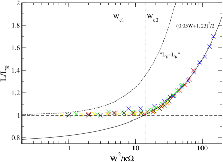
Figure 1: The experimental results of Swanson, Barenghi & Donnelly (1983), read off from their Figure 3 and represented by crosses in the figure, are compared to the phenomenological model of Jou & Mongiovi (2004) discussed in the text. The determination of the various parameters in the model is discussed in Appendix B. Clearly, the model (given by the dashed line below $W_{c2}$ and the solid curve above it) describes the experimental results quite well.

This relatively simple model turns out to describe the experimental results quite well. There is a flat region in $L$ below $W_{c}$ and the anticipated quadratic behaviour above $W_{c}$. Reading off the experimental data from Figure 3 in Swanson, Barenghi & Donnelly (1983) (see also Appendix B) and rescaling to our dimensionless quantities we find that the results for different rotation rates are well represented by the model, see Figure 1. This is, in fact, a useful sanity check since it shows that the various coefficients do not depend on $W$ or $\Omega$ in a significant way. The figure also shows that, taking $L_{H}^{1/2}={\alpha_{1}\over\beta}{W\over\kappa}$, we have $L<L_{H}+L_{R}$. The model cannot account for the small step in $L$ observed at $W_{c1}$ but for our present purposes this may not be very important.

Given the apparent success of this relatively simple model it would be interesting to apply it to the neutron star problem. Then we first of all need to be able to determine the various new coefficients. To arrive at some reasonable values is relatively easy. First compare (64) to (42) to see that

$$\alpha_{1} = \chi_{1}{\cal B}$$ (69)

$$\beta = {\chi_{2}\over 2\pi}$$ (70)

Next consider the slow-rotation limit where one would expect the vortex array to be straight. Then $L=L_{R}$ which means that

$$\beta_{2}=\sqrt{2}\alpha_{1}$$ (71)

The final two coefficients are obtained from (65) and the identification of $W_{c}$ with the critical velocity for the onset of the Donnelly-Glaberson instability $W_{DG}=2(2\nu\Omega)^{1/2}$. This leads to

$$\beta_{1} = {\chi_{2}\over\pi}-4\left({\nu\over\kappa}\right)^{1/2}\chi_{1}{\cal B}\approx 2\beta$$ (72)

$$\alpha_{2} = \sqrt{2}\left[{\chi_{2}\over\pi}-2\left({\nu\over\kappa}\right)^{1/2}\chi_{1}{\cal B}\right]\approx 2\sqrt{2}\beta$$ (73)

since ${\cal B}\ll 1$.

7.2 A phenomenological approach to the neutron star problem

Now that we have a basic picture of the combined problem of rotation and relative flow, we can try to formulate a prescription for turbulence in a rotating superfluid neutron star. By necessity, this will require a considerable leap of faith. After all, the Helium problem is not completely understood and in that case one has the luxury of being able to carry out laboratory studies. What hope do we have of making progress on the neutron star problem? We believe there are reasons to be optimistic. After all, a new perspective on superfluid dynamics is emerging and it will be quite exciting to see if even a very basic phenomenological model can help us understand observed phenomena, eg. related to glitches.

We want to work at the macroscopic fluid dynamics level, combining our description of mutual friction for a straight vortex array (8) with that for a vortex tangle (42) in a “sensible” way. To do this we will assume that we can average over the collection of vortices in each fluid element. In the presence of a turbulent vortex tangle we will assume that the averaging can be done on a lengthscale large enough that each fluid element contains an isotropic tangle as well as a “polarised” set of vortices that can be represented by a (locally) straight vortex array.

Combining what we have learned from the Helium problem, a ”workable” strategy might be as follows. First note that the turbulent vortex tangle does not contribute to $\nabla\times\vec{v}_{\rm n}$, while the polarised piece obviously does. Neglecting entrainment, which is difficult to account for in this phenomenological model, we let the average

$$\langle\nabla\times\vec{v}_{\rm n}\rangle=2\vec{\omega}_{\rm n}=n_{v}\vec{\kappa}$$ (74)

define the vorticity $\vec{\omega}_{\rm n}$ on the macroscopic scale. Taking the absolute value of this we can then identify

$$|\langle\nabla\times\vec{v}_{\rm n}\rangle|=2\omega_{\rm n}=L_{R}\kappa\ ,\quad\mbox{ that is }\quad L_{R}={1\over\kappa}|\langle\nabla\times\vec{v}_{\rm n}\rangle|\ ,\quad\mbox{ and}\quad n_{v}=L_{R}$$ (75)

We simply associate the vortex line length due to the local rotation $L_{R}$ with the density of straight vortices per unit area. Finally we make contact with the model discussed in the previous section by taking $\Omega=\omega_{\rm n}$.

Next we need the relative flow $W$ in (64). In the Helium experiment this is the counterflow along the rotation axis. Hence it seems natural to represent it by the projection of the relative flow $w^{{\rm n}{\rm p}}_{i}$ along the local rotation “axis”. This means that we would have

$$W=|\vec{w}_{{\rm n}{\rm p}}\cdot\hat{\omega}_{\rm n}|=|\vec{w}_{{\rm n}{\rm p}}\cdot\hat{\kappa}|$$ (76)

Here we have assumed that $W>0$. This is not a physical assumption, in fact, there is no reason why the flow should not be in a direction opposite to the rotation axis. However, we need to introduce this restriction to keep contact with (64).

Now we have all the ingredients required to work out the total line length $L$ per unit volume. First we should check if the relative flow exceeds the critical velocity for the onset of turbulence $W_{c}$. If it does not, then the sample is not turbulent and it is appropriate to use the Hall-Vinen form for the mutual friction (8). If, on the other hand, $W>W_{c}$ then we need a prescription for working out $L$. Provided that we can assume that the system is in “equilibrium” this is easy, and the required solution is given by (67). From this solution we readily deduce the total line length in the turbulent tangle $L_{T}=L-L_{R}$. Explicitly, we would have

$$L_{T}=\left({\alpha_{1}\over\beta}{W\over\kappa}\right)^{2}+{\alpha_{1}\beta_{1}\over\beta^{2}}{W\over\kappa}L_{R}^{1/2}+\left[{1\over 4}\left({\beta_{1}\over\beta}\right)^{2}-1\right]L_{R}$$ (77)

This allows us to work out the mutual friction due to the tangle by using $L_{T}$ in (37). Finally, the contribution from the polarised part follows from combining (8) with the deduced vortex density $n_{v}=L_{R}$. The combined mutual friction force for the polarised turbulent state (obviously only relevant above the critical velocity) can then be written

$$f_{i}^{\rm mf}=\rho_{\rm n}L_{R}\left\{{\cal B}^{\prime}\epsilon_{ijk}\kappa^{j}w_{{\rm n}{\rm p}}^{k}+{\cal B}\epsilon_{ijk}\epsilon^{klm}\hat{\kappa}^{j}\kappa_{l}w^{{\rm n}{\rm p}}_{m}-\tilde{\nu}\left[{\cal B}^{\prime}\hat{\kappa}^{j}\nabla_{j}\kappa_{i}+{\cal B}\epsilon_{ijk}\kappa^{j}\hat{\kappa}^{l}\nabla_{l}\hat{\kappa}^{k}\right]\right\}+{2L_{T}\over 3}\rho_{\rm n}\kappa{\cal B}w^{{\rm p}{\rm n}}_{i}\ .$$ (78)

This model represents what we think may be the simplest “reasonable” approach to the problem of superfluid neutron star turbulence. It has all the key ingredients, combining the standard straight vortex mutual friction with a contribution from an isotropic turbulent tangle. The main additional advantage is that all the steps can actually be worked out in a practical situation. Of course, the model is phenomenological and comes with a number of (potentially serious) caveats. Obviously, when we write down (77) we assume that the system is in equilibrium. This does not have to be the case. If one expects the timescale for reaching equilibrium to be long, then one can instead assume that $L$ evolves according to (64). The assumption that $W>0$ may also need to be relaxed. This can be done by considering the directionality in the problem in more detail. There have been some efforts to do this in the Helium case, see for instance Nemirovskii & Fiszdon (1995), Lipniacki (2001) and Jou & Mongiovi (2005). Common to the ideas discussed in these papers is the use of the Onsager symmetry principle to ensure that the second law of thermodynamics is honoured. This is important since the system is dissipative. An interesting approach to the problem was outlined in a series of papers by Geurst (1988, 1989, 1992) and Geurst & van Beelen (1994, 1995, 1996). The formalism developed in these papers seems particularly promising given that the equations for the basic two-fluid system are derived from a variational principle similar to that used by Prix (2004). An additional “fluid”, represented by the scalar density $L$ and the flow $\vec{v}_{L}$, is introduced to describe the turbulent tangle. This seems like a natural approach to take and there could be a considerable overlap with the general framework for dissipative multi-fluid systems recently developed by two of us (Andersson & Comer, 2006). We are planning to investigate this possibility in detail in the future.

8 Concluding remarks

We have discussed the problem of turbulence and the associated mutual friction force in a superfluid neutron star core. Our analysis was heavily influenced by work done on the analogous problem for superfluid Helium over the last 50 years, starting with the seminal work of Feynman (1955) and Vinen (1957). Focussing on the aspects of the problem that should be relevant for neutron stars, we have derived the form of the mutual friction force that should apply if the system becomes completely turbulent. We then argued that the neutron star case is likely to require an understanding of polarised turbulence, where rotation has a stabilising influence on the ability of relative flow to induce turbulence. In recognition of this, we formulated a phenomenological model that represents a first attempt (for neutron stars) to combine the presence of local rotation (represented by a “straight” vortex array”) and turbulence (an isotropic vortex tangle).

These results are intriguing, and possibly quite important. It will certainly be interesting to consider the effects that turbulence may have on, for example, pulsar glitch relaxation and neutron star oscillations. Having said that, we appreciate that this was our very first attempt at understanding the turbulence problem. The analysis may have taken us some way towards the solution to the problem, but more than likely we are only beginning to understand what the real questions are.

Appendix A: The induced flow for a curved vortex

Let us focus on a single vortex. In other words, we assume that the vortices are well separated, which implicitly puts some restrictions on the vortex curvature. To describe the vortex we take $s_{i}(\xi,t)$, where $\xi$ is a parameter denoting position along the vortex (essentially the arc length), as the position vector of the vortex from an arbitrary origin. The situation is illustrated in Figure 2 and it is useful to note that

$$s_{i}^{\prime} = {ds_{i}\over d\xi}=\hat{\kappa}_{i}$$ (79)

$$s_{i}^{\prime\prime} = {d^{2}s_{i}\over d\xi^{2}}={\rm s}^{\prime j}\nabla_{j}{\rm s}_{i}^{\prime}$$ (80)

A prime represents a derivative with respect to $\xi$. It is also useful to note the alternative form

$$s_{i}^{\prime\prime}=-\epsilon_{ijk}s^{\prime j}\epsilon^{klm}\nabla_{l}s^{\prime}_{m}$$ (81)

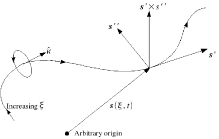
Figure 2: A schematic illustration of the variables used to describe the self-induced flow of a superfluid vortex.

To determine the self-induced velocity we must solve for the flow associated with the vortex. To do this we first note that it is the circulation of momentum $\bar{p}_{i}$ that is quantised (as in the main text, we distinguish the mesoscopic momentum by a bar), not that of velocity. As discussed in detail by Andersson, Sidery & Comer (2006) this is an important distinction to make once we include the entrainment. We need to solve (omitting for the moment any constituent indices)

$${1\over m}\epsilon_{ijk}\nabla^{j}\bar{p}^{k}=\kappa_{i}={h\over 2m}\hat{\kappa}_{i}$$ (82)

We can write down a formal solution in terms of a Green’s function by introducing a vector potential such that

$$\epsilon_{ijk}\nabla^{j}{A}^{k}={1\over m}\bar{p}_{i}$$ (83)

Using the associated gauge freedom to set

$$\nabla^{j}{A}_{j}=0$$ (84)

we see that we need to solve a vector Poisson equation;

$$\nabla_{j}\nabla^{j}{A}_{i}=-{\kappa}_{i}$$ (85)

The formal solution is given by

$$A_{i}(\vec{x})={1\over 4\pi}\int{\kappa_{i}\over|\vec{x}-\vec{y}|}d^{3}y$$ (86)

From this it follows that

$${\bar{p}_{i}(\vec{x})\over m}=-{1\over 4\pi}\int{\epsilon_{ijk}R^{j}\kappa^{k}\over R^{3}}d^{3}y$$ (87)

where $R^{i}=x^{i}-y^{i}$. To make use of this solution we note that $\kappa^{i}$ has support only on the vortex. Thus the volume integral collapses to a line integral along the vortex, in terms of $\xi$. Then we have $R^{i}=x^{i}-s^{i}$, and assuming that the vortex is only slightly bent we can make use of the Taylor expansion

$$s_{i}\approx s_{i}^{0}+s_{i}^{\prime}\xi+{1\over 2}s_{i}^{\prime\prime}\xi^{2}$$ (88)

This also leads to

$$\hat{\kappa}_{i}\approx s_{i}^{\prime}+s_{i}^{\prime\prime}\xi$$ (89)

Finally, we note that if we want to work out the corrections to the Magnus effect decribed by Andersson, Sidery & Comer (2006) we are interested in the induced flow in the vicinity of the vortex. This means that we take the limit $x^{i}\to s_{0}^{i}$, to arrive at

$$\epsilon_{ijk}R^{j}\hat{\kappa}^{k}\approx-{1\over 2}\epsilon_{ijk}s^{\prime j}s^{\prime\prime k}\xi^{2}$$ (90)

and

$${\bar{p}^{\mathrm{ind}}_{i}\over m}={\kappa\over 8\pi}\int{\epsilon_{ijk}s^{\prime j}s^{\prime\prime k}\over\xi}d\xi$$ (91)

To carry out the integration we introduce a cut-off at $\xi=a_{0}$, taken to be the size of the vortex core. This regularises the integral and also makes sense since we have not made any assumptions about the nature of the vortex core. We also introduce an upper limit $\xi=b$, assuming that the contribution to the induced flow can by localised to some part of the vortex. As a resonable value for $b$ one can use the intervortex separation. Finally, we arrive at the expression

$${\bar{p}^{\mathrm{ind}}_{i}\over m}={\kappa\over 4\pi}\log\left({b\over a_{0}}\right)\epsilon_{ijk}s^{\prime j}s^{\prime\prime k}\equiv\nu\epsilon_{ijk}s^{\prime j}s^{\prime\prime k}$$ (92)

In deriving this result we assumed symmetry with respect to $\xi=0$.

Appendix B. Determining the parameters in the phenomenological Helium model

The parameters used in Figure 1 were arrived at in the way discussed at the end of section 7.1. Specifically, we first take $L=L_{R}$ below the critical velocity. This fixes

$${\beta_{2}\over\alpha_{1}}=\sqrt{2}$$ (93)

A rough fit to the experimental results allows us to determine, cf. (67),

$${\alpha_{1}\over\beta}\approx 5\times 10^{-2}$$ (94)

and

$${\alpha_{1}\over\beta}{\beta_{1}\over\beta_{2}}\approx 1.23\rightarrow{\beta_{1}\over\beta_{2}}\approx 24.6$$ (95)

We can now combine these different estimates to get

$${\beta_{2}\over\beta}\approx 0.071$$ (96)

and then

$${\beta_{1}\over\beta}\approx 1.75$$ (97)

Next we assume that the critical velocity $W_{c2}$ corresponds to $W_{DG}$. This means that we should have $W_{c2}=2\sqrt{2\nu\Omega}$, or

$${\alpha_{2}\over\alpha_{1}}-2{\beta_{1}\over\beta_{2}}=2\sqrt{2\nu\over\kappa}$$ (98)

Combining this with the observed critical velocity $W_{c2}\approx 0.118\sqrt{\Omega}$ cm/s^1/2 we find that

$${\alpha_{2}\over\beta}\approx 2.65$$ (99)

We now have all parameters in (64) expressed in terms of $\beta$. The values we have deduced agree quite well with those used by Jou & Mongiovi (2004). Finally, we learn from Vinen (1957) that $\chi_{2}\approx 1$ which means that we could use

$$\beta={\chi_{2}\over 2\pi}\approx 0.16$$ (100)

Then all parameters in the model have been specified.

References

- Alpar, Langer & Sauls (1984) Alpar, M.A., Langer, S.A., Sauls, J.A., 1984, 282 533
- Alpar & Sauls (1988) Alpar, M.A., Sauls, J.A., 1988, Ap. J. 327 723
- Andersson (2003) Andersson, N., 2004, Class. Quantum Grav. 20 R105
- Andersson & Comer (2006) Andersson, N., Comer, G.L., 2006, Class. Quantum Grav. 23 5505
- Andersson, Sidery & Comer (2006) Andersson, N., Sidery, T., Comer, G.L., 2006, MNRAS 368 162
- Chevalier (1995) Chevalier, E., 1995, Europhys. Lett. 29 181
- Donnelly (1991) Donnelly, R.J., 1991, Quantized vortices in Helium II, Cambridge Univ. Press., Cambridge
- Feynman (1955) Feynman, R.P., 1955 in Prog. Low Temp. Phys., ed C.J. Gorter (North-Holland, Amsterdam), p. 17
- Finne et al (2003) Finne, A.P., Araki, T., Blaauwgeers, R., Eltsov, V.B., Kopnin, N.B., Krusius, M., Skrbek, L., Tsubota, M., Volovik, G.E., 2003, Nature, 424 1022
- Geurst (1988) Geurst, J.A., 1988, Physica B 153 166
- Geurst (1989) Geurst, J.A., 1989, Physica B 154 327
- Geurst (1992) Geurst, J.A., 1992, Physica A 183 279
- Geurst & van Beelen (1994) Geurst, J.A., van Beelen, H., 1994, Physica A 206 58
- Geurst & van Beelen (1995) Geurst, J.A., van Beelen, H., 1995, Physica B 205 209
- Geurst & van Beelen (1996) Geurst, J.A., van Beelen, H., 1996, Phys. Rev. B 54 6519
- Glaberson, Johnson & Ostermeier (1974) Glaberson, W.I., Johnson, W.W., Ostermeier, R.M., 1974, Phys. Rev. Lett. 33 1197
- Gorter & Mellink (1949) Gorter, C.J., Mellink, J.H., 1949, Physica 15 285
- Hall & Vinen (1956) Hall, H.E., Vinen, W.F., 1956, Proc. Roy. Soc. London A 238 215
- Henderson & Barenghi (2004) Henderson, K.L., Barenghi, C.F., 2004, Europhys. Lett. 67 56
- Jahan Miri (1998) Jahan Miri, M., 1998, Ap. J. Lett. 501 185
- Jones & Andersson (2001) Jones, D.I., Andersson, N., MNRAS 324 811
- Jou & Mongiovi (2004) Jou, D., Mongiovi, M.S., 2004, Phys. Rev. B 69 094513
- Jou & Mongiovi (2005) Jou, D., Mongiovi, M.S., 2005, Phys. Rev. B 72 144517
- Lindblom & Mendell (1995) Lindblom, L., Mendell, G., 1995, Ap. J. 444 804
- Lindblom & Mendell (2000) Lindblom, L., Mendell, G., 2000, Phys. Rev. D 61, 104003
- Lipniacki (2001) Lipniacki, T., 2001, Phys. Rev. B. 64 214516
- Lyne, Shemar & Graham Smith (2000) Lyne, A.G., Shemar, S.L., and Graham Smith, F., 2000, MNRAS 315 534
- Mendell (1991a) Mendell, G., 1991a, Ap. J. 380, 515
- Mendell (1991b) Mendell, G., 1991b, Ap. J. 380, 530
- Nemirovskii & Fiszdon (1995) Nemirovskii, S.K., Fiszdon, W., 1995, Rev. Mod. Phys. 67 37
- Packard (1972) Packard, R.E., 1972, Phys. Rev. Lett. 28 1080
- Peralta et al (2005) Peralta, C., Melatos, A., Giacobello, M., Ooi, A, 2005, Ap. J. 635 1224
- Peralta et al (2006) Peralta, C., Melatos, A., Giacobello, M., Ooi, A, 2006, Ap. J. 651 1079
- Prix (2004) Prix, R., 2004, Phys. Rev. D. 69 043001
- Schwarz (1982) Schwarz, K.W., 1982, Phys. Rev. Lett. 49 283
- Schwarz (1988) Schwarz, K.W., 1988, Phys. Rev. B 38 2398
- Swanson, Barenghi & Donnelly (1983) Swanson, C.E., Barenghi, C.F., Donnelly, R.J., 1983, Phys. Rev. Lett. 50 190
- Tsubota, Araki & Barenghi (2003) Tsubota, M., Araki, T., Barenghi, C.F., 2003, Phys. Rev. Lett. 90 205301
- Tsubota et al (2004) Tsubota, M., Barenghi, C.F., Araki, T., Mitani, A., 2004, Phys. Rev. B 69 134515
- Vinen (1957) Vinen, W.F., 1957, Proc. Roy. Soc. London A 240 493