Black Hole Shadow Image and Visibility Analysis of Sagittarius A*

Abstract

The compact dark objects with very large masses residing at the centres of galaxies are believed to be black holes. Due to the gravitational lensing effect, they would cast a shadow larger than their horizon size over the background, whose shape and size can be calculated. For the supermassive black hole candidate Sgr A*, this shadow spans an angular size of about 50 micro arc second, which is under the resolution attainable with the current astronomical instruments. Such a shadow image of Sgr A* will be observable at about 1 mm wavelength, considering the scatter broadening by the interstellar medium. By simulating the black hole shadow image of Sgr A* with the radiatively inefficient accretion flow model, we demonstrate that analyzing the properties of the visibility function can help us determine some parameters of the black hole configuration, which is instructive to the sub-millimeter VLBI observations of Sgr A* in the near future.

1 Introduction

There is compelling evidence that a $~{}4\times 10^{6}M_{\odot}$ black hole, associated with an extremely compact radio source Sagittarius A* (Sgr A*), resides at the Galactic Centre (Schödel et al., 2003; Ghez et al., 2005; Melia & Falcke, 2001). Recent Very Long Baseline Interferometry (VLBI) observations reveal that the intrinsic size of Sgr A* is only about 1 AU (Shen et al., 2005). For such a high degree of mass concentration, the relaxation time scale is much shorter than the age of our Galaxy, and thus almost all the theoretical models predict the formation of a supermassive black hole via gravitational collapse (Maoz, 1998).

However, to conclusively prove that Sgr A* is a supermassive black hole requires observations close to its event horizon, where relativistic effects can not be ignored. According to General Relativity, the photon trajectory will bend appreciably in a strong gravitational field (see, e.g., Misner, Thorne & Wheeler, 1973; Chandrasekhar, 1983). Because of this peculiar behavior, images of black holes and their immediate neighborhood we observe are highly distorted. The true physical structure in the very vicinity of the black hole must be decoded from the image via a ray tracing method (Fanton et al., 1997; Falcke, Melia & Agol, 2000; Schnittman & Bertschinger, 2004; Schnittman, Krolik & Hawley, 2006). In particular, if the impact parameter is smaller than a critical value, the photon is doomed to fall into the black hole (Chandrasekhar, 1983). As seen by a distant observer, this effect allows the black hole to cast a shadow over the background source that is larger than its event horizon.

The black hole candidate Sgr A*, at a distance of 8 kpc to us, spans an angular size of $\sim$ 20 micro arc second ($\mu$as) in diameter in the sky, which is beyond the resolution attainable with the current astronomical instruments. However, the shadow size is always of order $10GM/c^{2}$ in diameter, corresponding to an angular size of $50\mu$as for Sgr A*. In principle, this resolution can be achieved using VLBI techniques at a baseline length $\sim 4\times 10^{3}\rm{km}$ if observed at 1 mm wavelength (e.g., Falcke, Melia & Agol, 2000).

In this paper, we adopt the ray-tracing method to map the Sgr A* black hole with the radiatively inefficient accretion flow (RIAF) model (Yuan, Quataert & Narayan, 2003). We then use our simulations to estimate the visibility function to be observed by a VLBI array operating at, if can be designed in the future, sub-millimeter wavelengths. We are on the verge of resolving the shadow of the presumed supermassive black hole at the Galactic Centre.

The paper is organized as follows. Section $2$ briefly describes the formalism we use for the ray-tracing algorithm. We show the simulation results in Section $3$. Then we estimate the visibility functions in observations in Section $4$. Finally we give a discussion in Section $5$.

Throughout this paper, we will work with geometric units where $c=G=1$.

2 Hamiltonian Geodesic Ray-tracing in Black Hole Spacetime

In a given spacetime metric, the trajectory of a photon is uniquely determined by the initial conditions. To efficiently simulate the image of a black hole and its environment, we opt to impose our initial conditions at infinity, where the observer is, and integrate backwards in affine parameter toward the black hole (cf. Rauch & Blandford, 1994; Fanton et al., 1997). Starting from the standard kinetic Lagrangian, we compute the super-Hamiltonian (cf. Misner et al., 1973; Feng & Qin, 2003) in Kerr metric but with spin parameter $a=0$, since we discuss only the Schwarzschild black hole case in this work. Normal variational approach yields the Hamiltonian equations of motion in the phase space $(q^{\mu},p_{\mu})$, where $q^{\mu}$ and $p_{\mu}$ are Boyer-Linquist coordinate and the canonical momentum of the particle, respectively. If we choose the affine parameter to be proper time per unit rest mass (which has a finite limit even when the rest mass is zero in the photon case), then $p_{\mu}$ is interpreted as the covariant component of the four-momentum. Similar process can be seen in, e.g., Schnittman & Bertschinger (2004); Broderick & Loeb (2006).

As discovered by Bardeen et al. (1972), an infalling photon with its impact parameter (Chandrasekhar, 1983) less than $\sqrt{27}M$ will never escape the vicinity of the black hole. As seen by an outside observer, the black hole will cast a shadow of radius $r_{\text{shadow}}=\sqrt{27}M\approx 5.2M$ over the background light source. As reported by many numerical calculations (e.g., Falcke et al, 2000; Takahashi 2004), rotating black holes will cast shadows of approximately the same size as well.

In the following simulation, we specify initial conditions at a large distance (which we have chosen arbitrarily $r_{0}=200M$), and then integrate backward toward the black hole to obtain the full geodesic.

3 Results From Simulation

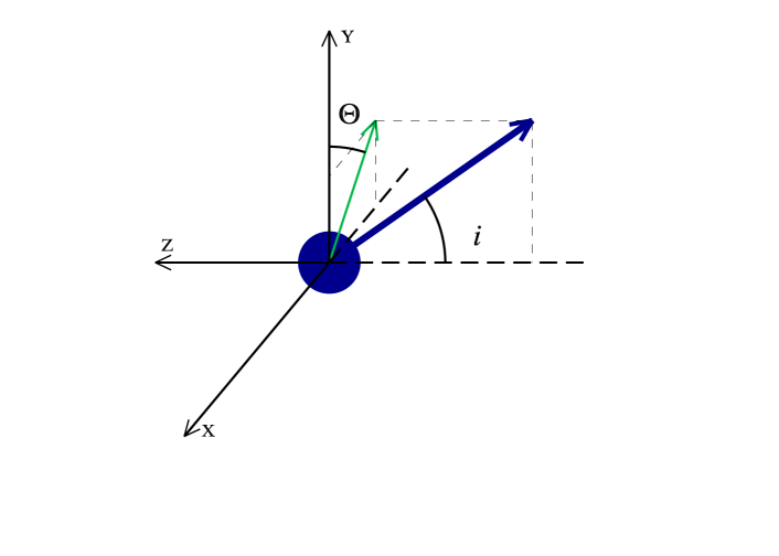
Figure 1: Sketch map of the black hole. $X$-axis is to east, $Y$-axis to north and $Z$-axis aligns with the line of sight of an observer. The blue arrow represents the direction of the black hole’s equatorial plane which is aligned with the mid-plane of the RIAF (see text), and $i$ and $\Theta$ are the inclination angle and position angle, respectively.

Fig. 1 is a sketch map, defining the inclination angle $i$ (Chandrasekhar, 1983) and position angle $\Theta$ used in our simulation. Three axes $(X,Y,Z)$ point east, north and the direction aligning with the line of sight for an observer, respectively. The thick blue arrow represents the direction of the black hole’s equatorial plane (the spin axis for the Kerr black hole). The inclination angle $i\in[-\pi/2,\pi/2]$ is the angle between the spin axis and the observer’s line of sight (Z axis), and the position angle $\Theta\in[-\pi,\pi]$ is the angle between the projection of spin axis on $X-Y$ plane and $Y$ axis, positive by east and negative by west. We limit $i\in[0,\pi/2]$ and $\Theta\in[-\pi/2,\pi/2]$ in the following discussion because of symmetry.

3.1 Black Hole Shadow of Sgr A* with the Radiatively Inefficient Accretion Flow Model

Even though there have been various theoretical models proposed to explain the observations of Sgr A* (see, e.g., Melia & Falcke, 2001), the precise structure of the dominant emitting region is still poorly known. In this paper, we only consider the RIAF model proposed by Yuan et al. (2003), which can satisfy most observational results including the observed spectrum of Sgr A* from radio to X-ray, the flaring activity at both infrared and X-ray bands, and its extremely faint luminosity.

In the RIAF model, the emission of Sgr A* from millimeter to sub-millimeter is dominated by the synchrotron radiation of thermal electrons. Thus one can determine the frequency-dependent emissivity $j_{\nu}(r,0)$ in the equatorial plane. Assuming a Gaussian distribution of electron density in the vertical direction of a RIAF, the emissivity distribution function is then:

$$j_{\nu}(r,z)=j_{\nu}(r,0)\exp(-\frac{z^{2}}{H^{2}}),$$ (1)

where $z$ is the vertical distance from the equatorial plane and $H$ is the scale height determined by:

$$H=\frac{\alpha_{s}}{\Omega_{\mathrm{K}}},$$ (2)

where $\alpha_{s}$ is the thermal sound speed and $\Omega_{\mathrm{K}}$ is the Keplerian angular velocity. The absorption coefficient $\kappa_{\nu}$ is then given by Kirchhoff’s Law. In this work, exactly the same RIAF model parameters in Yuan et al. (2003) and Yuan, Shen & Huang (2006) are adopted to preserve the good fit to the spectrum of Sgr A* and other observations.

To construct an observed emission structure, we then perform a full radiation transfer calculation using the ray-tracing method outlined in Section 2. Here, the radiative transfer equation takes the form:

$$\frac{dI_{\nu}}{ds}=j_{\nu}-\kappa_{\nu}I_{\nu}.$$ (3)

Since the frequency is red-shifted along the geodesic and $I_{\nu}/\nu^{3}$ is a Lorentz invariant (see, e.g., Chan et al., 2006; Schnittman et al., 2006; Noble et al., 2007), the observed specific intensity is related to the emitted intensity by

$$I_{\nu_{\rm{obs}}}=\delta^{3}I_{\nu_{\rm{em}}},$$ (4)

where the gravitational red-shift factor is calculated to be

$$\delta=\frac{\nu_{\rm{obs}}}{\nu_{\rm{em}}}={\sqrt{1-\frac{2M}{r}}}$$ (5)

for a non-spinning black hole. We neglect the re-emission process when solving the radiation transfer equation.

Furthermore, light rays emitted from the RIAF bend to us due to strong gravitation of the black hole, suffer absorption and in addition, suffer interstellar scattering. That means, what we can observe is a scatter-broadened image. The two-dimensional scattering structure in the direction to the Galactic Centre is determined from fitting to the angular size measurements as a function of the observing wavelength (cf. Shen et al., 2005). It is a Gaussian ellipse with full-widths at half maximum (FWHM) of major axis and minor axis in milli-arcsecond (mas) to be $(1.39\pm 0.02)\lambda^{2}$ and $(0.69\pm 0.06)\lambda^{2}$ ($\lambda$ measured in $\rm{cm}$), respectively and position angle $\sim 80^{\circ}$ (Shen et al., 2005). We take the conversion that one gravitation radius corresponds to $~{}5\mu$as angular size for Sgr A* with $4\times 10^{6}M_{\odot}$ mass at 8kpc distance.

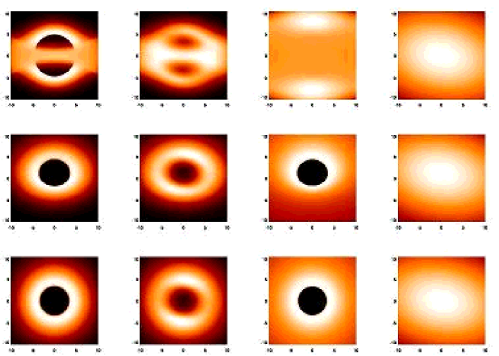
Figure 2: Simulated images of the RIAF of Sgr A* with $\Theta=0^{\circ}$ and $i=\pi/2,\pi/4,0$ (from top to bottom) at wavelengths of 1.3 mm (left two columns of panels) and 3.5 mm (right two columns of panels). For each two columns at two wavelengths, right one is obtained by convolving the left one (GR ray-tracing result) with the interstellar scattering. In each panel, the intensity is normalized to itself to show detailed structure. The units in the X- and Y-axes are gravitational radius $r_{g}$, which is 6$\times 10^{11}$ cm or 5$\mu$as for Sgr A* with $4\times 10^{6}M_{\odot}$ mass at 8 kpc distance.

In Fig. 2, we show both the un-scattered (ray-tracing only) and scatter-broadened images at wavelengths of 1.3 mm (first two columns of panels) and 3.5 mm (last two columns), respectively, obtained from our simulations with parameters $\Theta=0^{\circ}$, $i=\pi/2,\pi/4,0$ (from top to bottom). For each two columns at two wavelengths, right one is obtained by convolving the left one (GR ray-tracing result) with the interstellar scattering. We use color to show the self-normalized specific intensity of the images. The abscissa axes point to west and the ordinal axes point to north. The non-scattered (intrinsic) images are different at different wavelengths. They exhibit predicted shadows as a result of relativistic effects. The scattered image becomes more obscured as the observing wavelength increases. It indicates that gradually with the availability of the high-resolution VLBI imaging at wavelengths of 1.3 mm or shorter, we will be at a very good position to unveil the shadow structure of the black hole.

3.2 Comparison with the VLBI Observations at 7 and 3.5 mm

Currently, VLBI observations can be steadily performed at millimeter wavelengths of 3.5 and 7 mm. Attempts to determine the Sgr A* structure with the VLBI observations, however, have suffered from the angular broadening caused by the diffractive scattering by the turbulent ionized interstellar medium, which dominates the resultant images with a $\lambda^{2}$-dependence apparent size. The development of the model fitting analysis by means of the amplitude closure relation along with the careful design of the observations at millimeter wavelengths has greatly improved the accuracy of the size measurements of the observed image (e.g., Shen et al., 2003; Bower et al., 2004; Shen et al., 2005). As a result, an intrinsic source size as compact as 1 AU was first detected at 3.5 mm (Shen et al., 2005). However, for the reason discussed in Yuan et al. (2006), it is more meaningful to directly compare the observed apparent VLBI image with the scatter-broadened image obtained from the simulations. The apparent images of Sgr A* can be depicted quantitatively by an elliptical Gaussian distribution with the following parameters of the major and minor-axis sizes (Shen et al., 2005): 0.724$\pm$0.001 mas by 0.384$\pm$0.013 mas and 0.21${}^{+0.02}_{-0.01}$ mas by 0.13${}^{+0.05}_{-0.13}$ mas at wavelengths of 7 and 3.5 mm, respectively. The position angles at both wavelengths are about 80^∘, consistent with the orientation of the scattering structure.

While Yuan et al. (2006) only considered a special configuration, i.e., the RIAF is face-on ($i=0^{\circ}$ and $\Theta=0^{\circ}$), here we will do a thorough investigation on the possible geometry of the RIAF with respect to the presumed supermassive black hole in the Galactic centre based on the available VLBI measurements at both 3.5 and 7 mm. For this purpose, we first made a series of simulated after-scattering images with different geometric configuration (different combination of $i$ and $\Theta$) between the black hole and the RIAF. Then, we fit the simulated images with an elliptical Gaussian distribution to estimate the FWHMs of the major and minor axes.

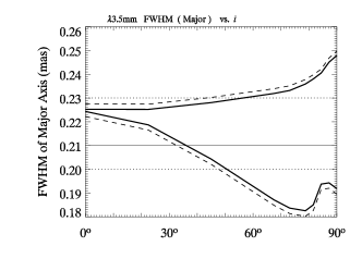
Figure 3: Comparison of the simulated sizes of Sgr A* with the real measurements at 7 mm (upper four panels) and 3.5 mm (lower four panels). Panels in left column, from top to bottom, show sizes (i.e. FWHMs) of the scatter-broadened images along directions of major axis at 7 mm, minor axis at 7 mm, major axis at 3.5 mm, and minor axis at 3.5 mm, as a function of the inclination angle ($i$) of the RIAF, while the panels in right column show these sizes as a function of the position angle ($\Theta$) of the RIAF. In each panel, the thick solid lines represent upper and lower limits of FWHMs of the images broadened by a constant scattering effect of 1.39$\lambda^{2}\times$0.69$\lambda^{2}$ with a position angle of 80^∘. The upper and lower limits to the sizes are due to different geometrical structure, i.e. different position angles at a fixed inclination angle $i$, or different inclination angles at a fixed position angle $\Theta$. After considering the uncertainties in the scattering angular sizes, the upper and lower limits are plotted with the thick dashed lines. The measured sizes and errors are represented by those straight thin solid and dotted lines.

In Fig. 3, the FWHMs of the major and minor axes of the simulated scattering-broadened images of Sgr A* are plotted as a function of the inclination angle ($i$) and the position angle ($\Theta$), respectively. Thick solid lines are the upper and lower limits of the FMHMs with the best-fit scattering angular size of 1.39$\lambda^{2}\times$0.69$\lambda^{2}$, and thick dashed lines are the upper and lower limits to account for the $\pm 1\sigma$ ($0.02\lambda^{2}\times 0.06\lambda^{2}$) in the scattering size. The measured angular sizes from high-resolution VLBA imaging (Shen et al., 2005) are indicated in Fig. 3 by the thin solid lines with the $1\sigma$ uncertainties by the thin dotted lines. As already shown in Yuan et al. (2006), within the uncertainties of the measurements and calculations, the predicted sizes from the RIAF model with $i=0^{\circ}$ and $\Theta=0^{\circ}$ are in reasonable agreement with the observations at two wavelengths. With a more thorough consideration shown in Fig. 3, it seems to suggest a geometry of the RIAF in Sgr A* to have a large inclination angle $i$ and a small position angle $\Theta$. But it should be cautious since the results in the minor axis are not accurate, especially at 3.5 mm (see, Shen et al., 2005). It is clear to us that in order to get a reliable estimate of the geometry ($i$ and $\Theta$) of the RIAF in Sgr A*, more accurate measurements are needed.

4 Visibility Functions of The Black Hole Shadow Images

As shown in Fig. 2 (also see Fig. 1 in Yuan, Shen & Huang, 2006), the simulated apparent scatter-broadened images of Sgr A* at wavelengths of 1.3 mm and shorter cannot be well fitted by one elliptical Gaussian component, indicating that the interstellar medium scattering effects at 1.3 and 0.8 mm no longer dominate the observed morphology. So, it is very promising to image the shadow of the supermassive black hole Sgr A* with the high-resolution VLBI observations at sub-millimeter wavelengths. However, there is no such a sub-millimeter VLBI array available at present for the imaging observations. Therefore, we will not focus on the comparison of the images at wavelengths of 1 mm and shorter, but try the visibility analysis to show that some useful constraints on the emission of Sgr A* can be extracted from the limited visibility data without imaging.

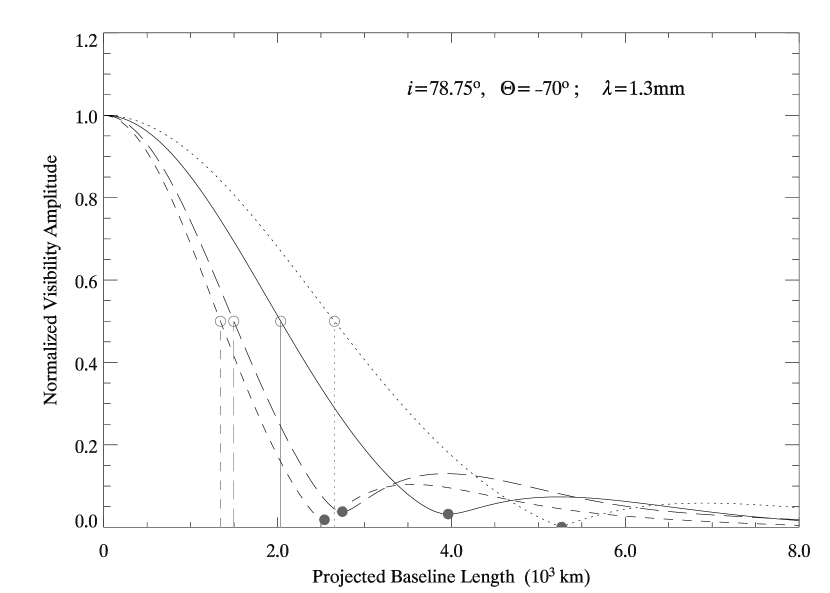
Figure 4: The predicted visibility function of Sgr A* (in this case, at 1.3 mm, with $i$=78.75^∘ and $\Theta$= $-70^{\circ}$). The four curves represent the normalized visibility amplitude profiles at four position angles, i.e. 80^∘ (solid line), $-10^{\circ}$ (long-dashed line), $35^{\circ}$ (short-dashed line) and $-55^{\circ}$ (dotted line). We mark where a profile reaches 0.5 (open circle) and its first valley (filled circle).

In the interferometric observation, the visibility function $V(u,v)$ measured on a baseline with coordinates $(u,v)$ is related, by the Fourier transform, to the sky brightness distribution, i.e., the shadow image in our simulation. To provide instructive information to the real observation, we first perform two-dimensional Fourier transform to obtain the visibility function of shadows like those in Fig. 2. Then we analyze the visibility distribution along four specific directions in the sky plane with position angles of (i) $80^{\circ}$ (E^′), i.e., along the major axis of the scattering structure; (ii) $-10^{\circ}$ (N^′), i.e., along the minor axis of the scattering structure; (iii) $35^{\circ}$ (NE^′); and (iv) $-55^{\circ}$ (NW^′). In Fig. 4, we show an example of such visibility slices with parameters, $i=78.75^{\circ}$ and $\Theta=-70^{\circ}$ at $\lambda=1.3\rm{mm}$. The abscissa is projected baseline length in the units of $10^{9}\lambda$ and the ordinate the normalized visibility amplitude. We plot slices in solid, long-dashed, short-dashed, and dotted line for E^′, N^′, NE^′, and NW^′ directions, respectively. To depict these visibility slices, we introduce two characteristic baseline lengths: $\Sigma$ (marked with open circle) to denote the baseline length at which a normalized visibility decreases to $0.5$, and $\sigma$ (marked with filled circle) to denote the baseline length at which the visibility reaches its first valley. Such a minimum in the visibility distribution is important because it implies that the image can no longer be described by a single Gaussian but must have an additional structure, which could be related to the black hole shadow. Visibilities at baselines longer than $\sigma$ have quite limited signal-to-noise ratio at millimeter wavelengths. The typical detection limit with the current VLBA (Very Long Baseline Array) at 3.5 mm is about $0.12$ mJy.

It is obvious that different sets of geometrical parameters ($i$ and $\Theta$) will result in different visibility profiles at different wavelengths. For a given orientation of the RIAF model at a given wavelength, we can obtain two characteristic baseline lengths ($\Sigma$ and $\sigma$) along each of the four directions (E^′, N^′, NE^′, and NW^′), i.e. ($\Sigma_{E^{\prime}}$, $\sigma_{E^{\prime}}$), ($\Sigma_{N^{\prime}}$, $\sigma_{N^{\prime}}$), ($\Sigma_{NE^{\prime}}$, $\sigma_{NE^{\prime}}$), and ($\Sigma_{NW^{\prime}}$, $\sigma_{NW^{\prime}}$). We further list these in the order of their lengths and denote them as $\Sigma_{n}$ and $\sigma_{n}$ with n=1 (the shortest) to 4 (the longest).

Our simulations show that the scattering effect at 3.5 mm is still quite large (see Fig. 2), thus we cannot get enough information of any fine structure of the shadow. To minimize the scattering effect, we consider the observations to be performed at other two shorter wavelengths 1.3 and 0.8 mm. Shown in Fig. 5 are the two characteristic baseline lengths ($\Sigma$ and $\sigma$) as a function of the inclination angle $i$ at 1.3 (upper two panels) and 0.8 mm (lower two panels). With a specific $i$, each of $\Sigma_{n}$ and $\sigma_{n}$ (n=1$-$4) can vary within a region due to the different position angle $\Theta$. These allowed regions for $\Sigma_{1}$, $\Sigma_{2}$, $\Sigma_{3}$, and $\Sigma_{4}$ (or, $\sigma_{1}$, $\sigma_{2}$, $\sigma_{3}$, and $\sigma_{4}$) are shown as the darkest grey with long-dashed border lines, lightest grey with dotted border lines, second lighter grey with short-dashed border lines, and white with solid border lines, respectively. From these plots, we summarize some useful properties as follows:

1. Most of the characteristic baseline lengths are in a range of (1$-4)\times 10^{3}~{}\rm{km}$, which should be achievable under current VLBI observation conditions. Therefore, VLBI observations of Sgr A* at sub-millimeter wavelengths are expected to provide very important results in the near future. Some extreme cases may require a project baseline length longer than 5$\times 10^{3}~{}\rm{km}$ for $\sigma_{4}$.

2. When the RIAF is nearly face-on ($i\approx 0^{\circ}$), the four $\Sigma$s (or $\sigma$s) are converged to a single similar number, suggesting that the four visibility profiles are almost identical and thus not orientation-dependent. This is mainly due to the isotropy of the intrinsic shadow image without scattering. The roughly East-West (80^∘ in position angle) elongated scattering structure is very compact, $\leq 15\mu$as along the major axis at about 1 mm wavelength, and thus will not affect the symmetry of the final scatter-broadened image.

3. With a moderate inclination angle $i$, the differences between these projected baselines at different directions are quite significant. In fact, the four $\Sigma$s (or $\sigma$s) are always range in four separate regions (as shown in Fig. 5) because of the asymmetry of the image. The possible region, caused by the different position angle $\Theta$, for each $\Sigma$ and $\sigma$ becomes larger when the inclination angle $i$ increases.

Therefore, in principle we would be able to constrain the inclination angle ($i$) of the RIAF in Sgr A* by comparing the above-mentioned characteristic baseline lengths determined from the future 1.3 and/or 0.8 mm VLBI experiments with the simulation demonstrated in this paper. It can be inferred from Fig. 5 that when the RIAF has a large inclination angle (in our simulation of Sgr A*, $i>\sim 30^{\circ}$), both $\Sigma$s and $\sigma$s become very sensitive to $\Theta$.

No wonder, the position angle $\Theta$ should have effects on the characteristic baseline lengths too. For clarity, we define here another three normalized differences in the characteristic baseline lengths:

$$S_{1} = (\Sigma_{N^{\prime}}-\Sigma_{E^{\prime}})/(\Sigma_{4}-\Sigma_{1}),$$

$$S_{2} = (\Sigma_{NE^{\prime}}-\Sigma_{NW^{\prime}})/(\Sigma_{4}-\Sigma_{1}),$$ (6)

$$S_{3} = (\Sigma_{E^{\prime}}-\Sigma_{NE^{\prime}})/(\Sigma_{4}-\Sigma_{1}).$$

Note that $\Sigma_{4}$ and $\Sigma_{1}$ represent the longest and shortest characteristic baseline lengths, respectively. If the RIAF is nearly face-on ($i\approx 0^{\circ}$), the scatter-broadened image of Sgr A* is roughly E-W elongated, resulting in the $\Sigma_{N^{\prime}}$ being the longest and $\Sigma_{E^{\prime}}$ the shortest (i.e., $\Sigma_{N^{\prime}}$=$\Sigma_{4}$ and $\Sigma_{E^{\prime}}$=$\Sigma_{1}$), and $\Sigma_{NE^{\prime}}$=$\Sigma_{NW^{\prime}}$ because of its symmetry. Therefore, it is always the case that $S_{1}=1$, $S_{2}=0$ and $-1<S_{3}<0$ for any $\Theta$. This means the face-on case is not sensitive to the position angle, consistent with the almost identical characteristic baseline lengths shown in Fig. 5 when $i\approx 0^{\circ}$.

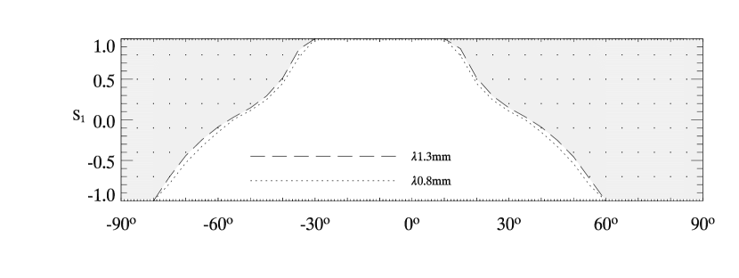
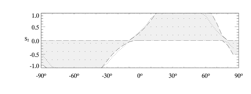
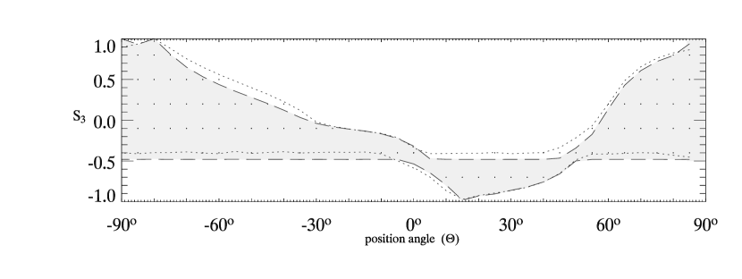
Figure 6: The normalized difference of the characteristic baseline lengths ($S_{1}$, $S_{2}$, and $S_{3}$, from top to bottom) as a function of the position angle $\Theta$. For a given position angle ($\Theta$), $S_{1}$, $S_{2}$, and $S_{3}$ can vary with the inclination angle $i$, and have a range represented by the grey region with dashed border lines and the dotted region with dotted border lines for observations at 1.3 and 0.8 mm, respectively.

Shown in Fig. 6 are plots of $S_{1}$, $S_{2}$ and $S_{3}$ as a function of the position angle ($\Theta$). At a given position angle $\Theta$, these values vary with the inclination angle $i$ and have a range represented by grey region with dashed border lines (at 1.3 mm) and dotted region with dotted border lines (at 0.8 mm).

Assuming that the RIAF model is a physically reasonable description of the observed emission of Sgr A*, our simulation indicates that starting with the limited visibility measurements on the four baselines in the directions mentioned above from the future sub-millimeter (1.3 and 0.8 mm) VLBI experiments, we have a very good chance to get tight constraints on the configuration ($i$ and $\Theta$) of the RIAF around the central supermassive black hole of Sgr A*. That is, we can understand the geometry of the radio-emitting region surrounding Sgr A* in advance, even without imaging it with a completely $(u,v)$ coverage of sub-millimeter/millimeter VLBI array. It is important to indicate that the detection of $\sigma$s, i.e., valleys in the visibility profile (see Fig. 4 and Fig. 5) , are very important to prove that there is indeed a supermassive black hole in the centre of our Galaxy.

5 Discussion and Summary

With the emissivity and absorption coefficient from the radiatively inefficient accretion flow model for the Galactic Centre black hole candidate Sgr A*, we solved the radiative transfer using the ray-tracing code to get the simulated shadow images of Sgr A* with an arbitrary set of geometrical parameters, i.e., $i$ and $\Theta$. By taking into account the interstellar scattering, we can obtain the apparent images at different wavelengths.

Comparison of the simulated image sizes with those measurements at both 7 and 3.5 mm seems to prefer a RIAF with a large inclination angle and small position angle for Sgr A*. But, large uncertainties in both the size measurements and the interstellar scattering relationship make these very uncertain at the moment. Even though, our simulations show that the future sub-millimeter VLBI images of Sgr A* would reveal a significant deviation from the single Gaussian structure, which can be used to probe the geometry of the RIAF of Sgr A*.

Analysis of the scatter-broadened images also show that an observing wavelength of 1.3 mm or shorter is needed to identify the shadow shape. However, currently it is difficult to construct a VLBI array operated at 1.3 mm to obtain such an image. We therefore first perform the Fourier transform to obtain the corresponding visibility functions of images at 1.3 and 0.8 mm, then analyze these visibility profiles along some specific directions. By introducing several characteristic baseline lengths ($\Sigma_{n}$ and $\sigma_{n}$) and the normalized differences ($S_{n}$), we demonstrate that it is possible to determine fundamental parameters ($i$ and $\Theta$) of Sgr A* from the limited detections on some baselines of VLBI observations at a wavelength of 1 mm or shorter (cf. Fig. 5 and Fig. 6). We can understand the geometry of the radio-emitting region surrounding Sgr A* even without imaging it with a completely $(u,v)$ coverage of a sub-millimeter/millimeter VLBI array.

It should be mentioned that the four directions chosen in our analysis are somehow arbitrary. Any other combinations would also provide useful constraints on the structure of Sgr A*. For example, it would be interesting to choose such two specific slices, one along the galactic plane and the other perpendicular to it. In practice, we can perform the similar simulations with the projected baselines to be exactly the same as those from the real sub-millimeter VLBI experiments in the future. Of course the RIAF model adopted here is still quite simple. We set the static black hole, use Pseudo-Newtonian potential (Yuan et al., 2003), and simply assume a Gaussian distribution of the density as the vertical structure of the accretion flow. And the possible dynamical role of an ordered magnetic field is not considered. We also neglect the Doppler effect of the radial and angular motions of the accretion flow in the radiative transfer calculation. However in principal, the visibility analysis outlined in this paper should be applicable, even if Sgr A* is a spinning black hole or with other accretion flow geometries and emission models. As a necessary first step trying to solve this complicated problem, this work definitely needs further efforts in both modelling and observations. And a more quantitative study will be required in future work.

Furthermore, that the characteristic baseline lengths are about $10^{3}$ km and the expected observing wavelength is about 1 mm encourage us to propose the development of sub-millimeter VLBI array. The image of the vicinity of the predicted black hole in Sgr A* is expected to be more easily detected than any other super-massive black hole candidates because of its closest distance to us. If the shadow image could be finally observed, it will be strong evidence for the General Relativity theory.

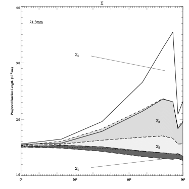
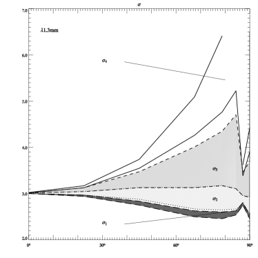
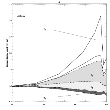
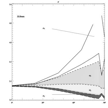
Figure 5: The projected characteristic baseline lengths versus the inclination angle $i$ at 1.3 mm (upper two panels) and 0.8 mm (lower two panels). With a specific inclination angle $i$, each of $\Sigma_{n}$ and $\sigma_{n}$ (n=1-4) can vary with the position angle $\Theta$. These allowed regions for $\Sigma_{1}$, $\Sigma_{2}$, $\Sigma_{3}$, and $\Sigma_{4}$ (or, $\sigma_{1}$, $\sigma_{2}$, $\sigma_{3}$, and $\sigma_{4}$) are shown as the darkest grey with long-dashed border lines, lightest grey with dotted border lines, second lighter grey with short-dashed border lines, and white with solid border lines, respectively.

References

- Bardeen et al. (1972) Bardeen J.M., Press W.H., Teukolsky S.A., 1972, ApJ, 178, 347
- Bower et al. (2004) Bower G. C., Falcke H., Herrnstein R. M., Zhao J., Goss W. M., Backer D. C. 2004, Sci, 304, 704
- Broderick & Loeb (2006) Broderick A.E., Loeb A., 2006, MNRAS, 367, 905
- Chan et al. (2006) Chan C.K., Liu S., Fryer C.L., Psaltis D., Özel F., Rockefeller G., Melia F., 2006, astro-ph/0611269
- Chandrasekhar (1983) Chandrasekhar S., 1983, The Mathematical Theory of Black Holes, Oxford Univ. Press, Oxford
- Falcke et al. (2000) Falcke H., Melia F., Agol E., 2000, ApJ, 528, 13
- Fanton et al. (1997) Fanton C., Calvani M., Felice F., Cadez A. 1997, PASJ, 49, 159
- Feng & Qin (2003) Feng K., Qin M.-Z., 2003, Symplectic Geometric Algorithms For Hamiltonian System, Zhejiang Science & Technology Press, Hangzhou.
- Ghez et al. (2005) Ghez A.M., Salim S., Hornstein S.D., Tanner A. Lu J.R., Morris M., Becklin E., Duchene G., 2005, ApJ, 620, 744
- Maoz (1998) Maoz E., 1998, ApJ. 494, L181
- Melia & Falcke (2001) Melia F., Falcke H., 2001, ARA&A, 39, 309
- Misner et al. (1973) Misner C.W., Thorne K.S.,Wheeler J.A., 1932, Gravitation, W.H.Freeman & Company, San Francisco
- Narayan & Yi (1994) Narayan R., Yi I., 1994, ApJ, 428, L13
- Noble et al. (2007) Noble S.C., Leung P.K., Gammie C.F., Book L.G., 2007, astro-ph/0701778
- Rauch & Blandford (1994) Rauch K.P., Blandford R.D., 1994, ApJ, 421, 46
- Schnittman & Bertschinger (2004) Schnittman J.D., Bertschinger E., 2004, ApJ, 606, 1098
- Schnittman et al. (2006) Schnittman J.D., Krolik J.H., Hawley J.F., 2006, ApJ, 651, 1031
- Schödel et al. (2003) Schödel R., Ott T., Genzel R., Eckart A., Mouawad N., Alexander T., 2003, ApJ, 596, 1015
- Shakura & Sunyaev (1973) Shakura N.I., Sunyaev R.A., 1973, A&A, 24, 337
- Shen et al. (2003) Shen Z.-Q., Liang M.C., Lo K. Y., Miyoshi M., 2003, Astron. Nachr., 324, S1, 383
- Shen et al. (2005) Shen Z.-Q., Lo K.Y., Liang M.C., Ho P.T.P., Zhao J.H., 2005, Nat, 438, 62
- Takahashi (2004) Takahashi R., 2004, ApJ, 611, 996
- Yuan et al. (2003) Yuan F., Quataert E., Narayan R., 2003, ApJ, 598, 301
- Yuan et al. (2006) Yuan F., Shen Z.-Q., Huang L., 2006, ApJ, 642, L145