The cross-correlation between galaxies of different luminosities and colors

Abstract

We study the cross-correlation between galaxies of different luminosities and colors, using a sample of 284489 galaxies selected from the Sloan Digital Sky Survey, Data Release 4. Galaxies are divided into 6 samples according to luminosity, and each of these samples is further divided into red and blue subsamples according to their $(g-r)$ colors. Projected auto-correlation is estimated for each subsample, and projected cross-correlation is estimated for each pair of subsamples. At projected separations $r_{p}\gtrsim 1\>h^{-1}{\rm{Mpc}}$, all correlation functions are roughly parallel, although the correlation amplitude depends systematically on both luminosity and color. On $r_{p}\lesssim 1\>h^{-1}{\rm{Mpc}}$, the auto- and cross-correlation functions of red galaxies are significantly enhanced relative to the corresponding power laws obtained on larger scales. Such enhancement is absent for blue galaxies and in the cross-correlation between red and blue galaxies. We estimate the relative bias factor on scales $r\gtrsim 1\>h^{-1}{\rm{Mpc}}$ for each subsample using its auto-correlation function as well as its cross-correlation functions with other subsamples. The relative bias factors obtained from different methods are similar. For blue galaxies the luminosity-dependence of the relative bias is strong over the entire luminosity range probed ($-23.0<M_{r}\leq-18.0$), while for red galaxies the dependence is weaker and becomes insignificant for luminosities below $L^{*}$. In order to examine whether a significant stochastic/nonlinear component exists in the bias relation, we study the ratio ${\cal R}_{ij}\equiv W_{ii}W_{jj}/W_{ij}^{2}$, where $W_{ij}$ is the projected correlation between subsample ‘$i$’ and ‘$j$’. We find that the values of ${\cal R}_{ij}$ are all consistent with 1 for all-all, red-red and blue-blue samples, however significantly larger than 1 for red-blue samples. For faint red - faint blue samples the values of ${\cal R}_{ij}$ are as high as $\sim 3$ on small scales ($r_{p}\lesssim 1\>h^{-1}{\rm{Mpc}}$) and decrease with increasing $r_{p}$. These results suggest that a significant stochastic/nonlinear component exists in the relationship between red and blue galaxies, particularly on small scales.

1. Introduction

In the current scenario of structure formation, galaxies are assumed to form in the cosmic density field through a series of physical processes, such as non-linear gravitational collapse, gas cooling and star formation. In this scenario the distribution of galaxies in space is expected to trace the underlying density field to some degree, but the relationship is not expected to be perfect, because many of the processes involved in galaxy formation can complicate the relationship between galaxies and the dark matter density field. Thus, the study of galaxy clustering in space is an important step both in understanding the mass distribution in the universe, and in understanding how galaxies form in the cosmic density field. The statistical tool commonly adopted to quantify galaxy clustering in space is the correlation functions of galaxies (Peebles 1980). During the last two decades, many authors have estimated the two-point correlation functions of galaxies using various redshift catalogs, to study how galaxy clustering depends on the properties of galaxies, such as luminosity (e.g. Börner, Mo & Zhou 1989; Park et al. 1994; Loveday et al. 1995; Guzzo et al. 1997; Benoist et al. 1996; Norberg et al. 2001; Zehavi et al. 2002; Zehavi et al. 2005; Li et al. 2006), color (e.g. Willmer et al. 1998; Brown et al. 2000; Zehavi et al. 2002; Zehavi et al. 2005; Li et al. 2006), spectral type (Norberg et al. 2002; Budavari et al. 2003; Madgwick et al. 2003), morphological type (e.g. Jing, Mo & Börner 1991; Guzzo et al. 1997; Willmer et al. 1998; Zehavi et al. 2002; Goto et al. 2003), stellar mass, stellar surface mass density and concentration (Li et al. 2006). All these analyses show that galaxies of different properties may have different distributions in space, indicating that galaxies are biased tracers of the underlying density field and that one has to be careful when using the observed galaxy distribution to infer the mass distribution in the universe.

The observed correlation functions of galaxies can provide important constraint on the relationship between galaxies and dark matter halos, as is demonstrated clearly in the recent halo-occupation and conditional-luminosity-function models (Jing, Mo & Börner 1998; Seljak 2000; Peacock & Smith 2000; Berlind & Weinberg 2002; Cooray & Sheth 2002; Yang, Mo & van den Bosch 2003; van den Bosch, Yang & Mo 2003). With accurate measurements of the clustering properties for galaxies of different properties, it is now possible to study in great detail how different galaxies occupy different halos and how galaxies trace the cosmic density field.

The correlation analyses carried out so far are mostly based on the auto-correlation function of galaxies. Although such analyses can provide important information about how a population of galaxies is distributed in space, they do not tell us anything about the relationship between galaxies of different properties. For example, two populations of galaxies may each be strongly clustered in space and yet be spatially segregated so that the cross-correlation between them is weak. In reality, all populations of galaxies may be biased tracers of the underlying mass distribution, and so they must all be positively correlated in space. However, the amplitude of the cross-correlation between any two populations of galaxies depends not only on the bias factors of these two populations, but also on how well each of them trace the mass density field, i.e. on the stochasticity in the bias relation. Thus, it is important to measure the cross-correlation functions between galaxies of different properties, so as to quantify the relationships between the spatial distributions of different galaxies.

In this paper, we use galaxy samples constructed from the Sloan Digital Sky Survey Data Release 4 (SDSS-DR4) to measure both the auto-correlation functions for galaxies of different luminosities and colors and the cross-correlation functions between different galaxies. We compare the shapes of the various correlation functions to check the validity of the assumption of linear bias. For each population of galaxies (i.e. for galaxies within given ranges of luminosity and color), we estimate its relative bias factors using its auto-correlation function as well all its cross-correlation functions with other populations of galaxies. These bias factors are averaged to give a mean bias factor for each population, and compared among themselves to constrain possible stochastic/nonlinear component in the bias relation (Mo & White 1996; Dekel & Lahav 1999). This paper is organized as follows. In section 2, we describe the galaxy samples to be used and how random samples are constructed. In section 3, we describe our method for estimating the correlation functions. Our results about the luminosity- and color-dependence of the correlation functions are presented in Sections 4 and 5, respectively. In Section 6 we discuss the implications of our results for the possible existence of stochastic/non-linear bias in galaxy distribution. Finally, we summarize our findings in Section 7.

Throughout this paper, galaxy distances are obtained from redshifts assuming a cosmology with $\Omega_{\rm m,0}=0.3$, $\Omega_{\Lambda,0}=0.7$. Distances are quoted in units of $\>h^{-1}{\rm{Mpc}}$, and absolute magnitudes are quoted in terms of $M-5\log h$, i.e. with $h$ set to be 1, where $h=H_{0}/(100{\rm kms^{-1}Mpc^{-1}})$.

2. The data

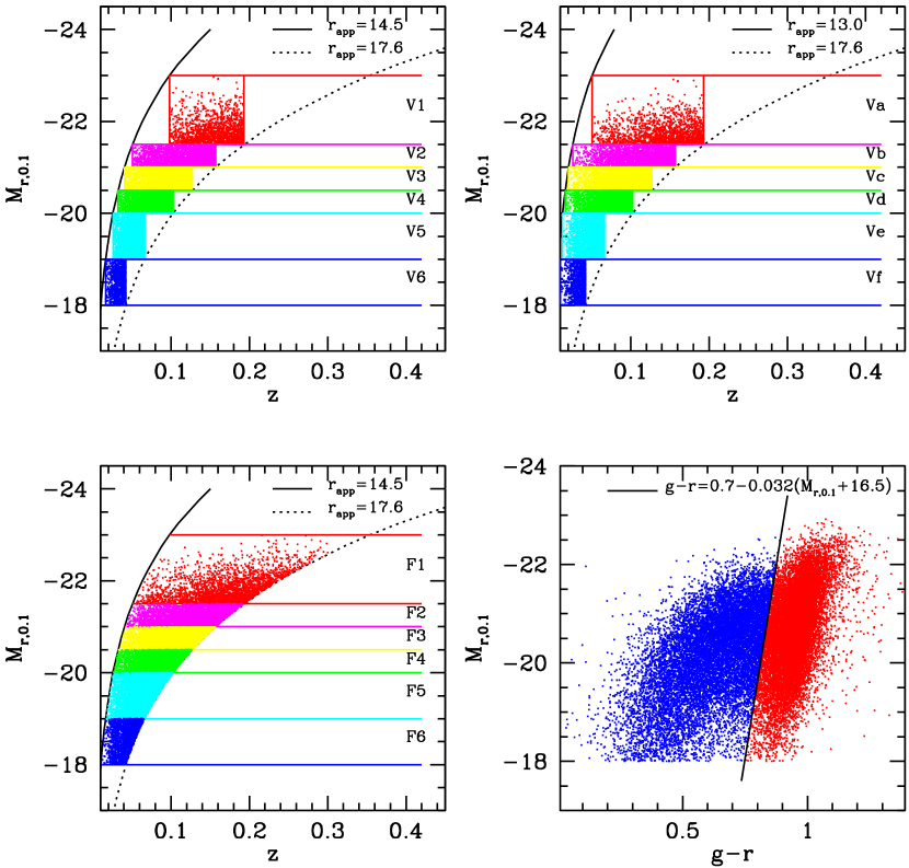
Figure 1.— The magnitude-redshift distributions of 10% galaxies in the volume-limited samples V1–V6 (upper left panel), Va – Vf (upper right panel) and flux-limited samples F1 – F6 (lower left panel). The lower right panel shows the color-magnitude distribution of $10\%$ of the main sample galaxies. The solid line $g-r=0.7-0.032(M_{r,0.1}+16.5)$ separates the galaxies into red and blue populations. See Tables  1 and  2 for more infomation.

2.1. The SDSS Data Release 4

Table 1Volume-limited samples

		Number of Galaxies
Sample	$M_{r,0.1}$	NGCE	NGCO	SGC	z
V1/Va	(-23.0, -21.5]	4670/5365	8935/10030	2704/3050	(0.098, 0.193)/(0.051, 0.193)
V2/Vb	(-21.5, -21.0]	9288/9485	16978/17442	4777/4919	(0.051, 0.157)/(0.026, 0.157)
V3/Vc	(-21.0, -20.5]	11833/12110	19987/20542	5676/5837	(0.041, 0.127)/(0.021, 0.127)
V4/Vd	(-20.5, -20.0]	10842/11158	17705/18348	5146/5317	(0.033, 0.103)/(0.017, 0.103)
V5/Ve	(-20.0, -19.0]	6493/6974	15462/16073	4317/4571	(0.026, 0.066)/(0.013, 0.066)
V6/Vf	(-19.0, -18.0]	2620/2690	5321/5485	1534/1590	(0.017, 0.043)/(0.010, 0.043)

Note. — Column 1 indicates the sample ID. Column 2 gives the absolute-magnitude range covered by each sample. Columns 3, 4 and 5 list the galaxy number in each sample in the three regions (NGCE, NGCO, SGC) of the SDSS. Column 6 lists the redshift range of each sample. Each sample is a volume-limited in the redshift range it covers. Samples V1 – V6 are for galaxies with $r$-band apparent magnitudes in the range from 14.5 to 17.6. Samples Va – Vf are constructed from all galaxies with $r$-band apparent magnitudes in the range from 13.0 to 17.6. The reason for using these two sets of volume-limited samples is given in the main text.

Table 2Flux-limited samples

		Number of Galaxies
Sample	$M$	NGCE (Red/Blue)	NGCO (Red/Blue)	SGC (Red/Blue)	$z$
F1 (${\rm F1_{red}}$/${\rm F1_{blue}}$)	(-23.0, -21.5]	8817 (7203/1614)	17012 (13745/3267)	5108 (4147/961)	(0.051, 0.300)
F2 (${\rm F2_{red}}$/${\rm F2_{blue}}$)	(-21.5, -21.0]	14189 (9173/5016)	26598 (17150/9448)	7556 (4938/2618)	(0.041, 0.193)
F3 (${\rm F3_{red}}$/${\rm F3_{blue}}$)	(-21.0, -20.5]	19025 (10968/8057)	33459 (19174/14285)	9498 (5434/4064)	(0.033, 0.157)
F4 (${\rm F4_{red}}$/${\rm F4_{blue}}$)	(-20.5, -20.0]	17214 (8979/8235)	29037 (15186/13851)	8329 (4271/4058)	(0.026, 0.127)
F5 (${\rm F5_{red}}$/${\rm F5_{blue}}$)	(-20.0, -19.0]	20252 (8949/11303)	36386 (15810/20576)	10162 (4369/5793)	(0.017, 0.103)
F6 (${\rm F6_{red}}$/${\rm F6_{blue}}$)	(-19.0, -18.0]	5597 (1409/4188)	12687 (3570/9117)	3563 (1041/2522)	(0.010, 0.066)
F*	(-20.7, -20.2]	18444	31714	8975

Note. — Similar to Table 1 but for flux-limited samples. Here again galaxies with $r$-band apparent magnitudes in the range from 14.5 to 17.6 are selected. Numbers are listed separately for all, red and blue galaxies. ${\rm F^{*}}$ is a sample of galaxies with luminosities within a $0.5$ magnitude bin around $L^{*}$.

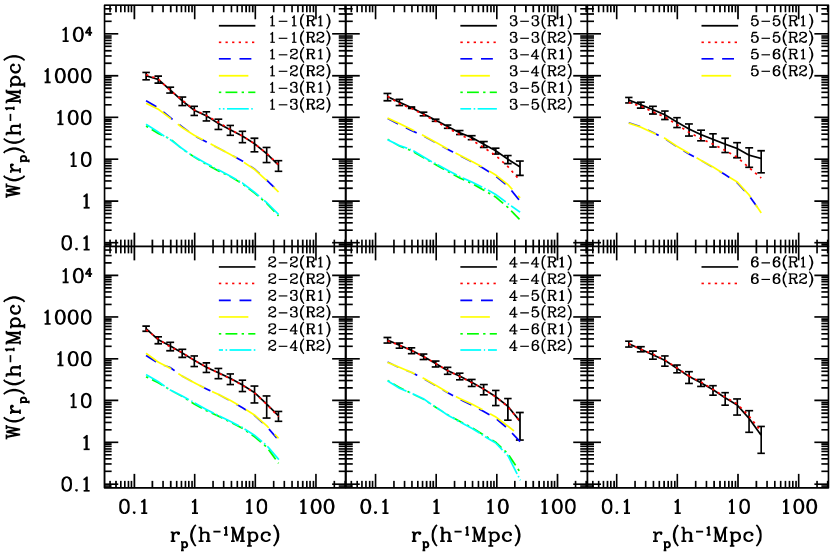
Figure 2.— The projected 2PCFs for the flux-limited samples. Here we compare the results obtained by using two different random samples, R1 and R2 (see the main text for how R1 and R2 are constructed). The error-bars in this plot represent the 1-$\sigma$ scatter among the three SDSS regions. For clarity, we only plot error-bars for the auto-correlation functions but note that the error-bars for the cross-correlation functions have similar sizes. The results for the cross-correlation functions are shifted downward by $0.5$ and $1$ dex for the cases Fi – F(i+1) and Fi-F(i+2) (i=1,2,3,4,5), respectively. Note that in most of the cases, these two types of random samples yield very similar results. However, discrepancy exists in a few cases, especially for the auto-correlation function of F5. As discussed in the main text, this discrepancy is likely caused by the supercluter at redshift $z\sim 0.08$.

In this paper we use galaxy samples constructed from the New York University Value-Added Galaxy Catalog (NYU-VAGC, see Blanton et al. 2005). The version of the NYU-VAGC used here is based on the SDSS Data Release 4 (Adelman-McCarthy et al. 2006 ) which consists of three regions: two in the Northern Galactic Cap (NGC) and one in the Southern Galactic Cap (SGC). We refer the two NGC regions separately as NGCE (which is along the celestial equator) and NGCO (which is off the equator). The SGC contains three stripes: one along the celestial equator, one to the north and one to the south. In this paper, we measure the correlation functions separately for NGCE, NGCO and SGC, and obtain the variance from these samples. While the total correlation functions of the whole samples are obtained by combining the pair counts in all these three regions. Note that these three regions have quite large angular separations which ensure us to obtain a good estimation of the cosmic variance, except for those faintest galaxies at very low redshift where the variance may be somewhat underestimated. Our main sample contains 284489 galaxies with extinction-corrected Petrosian magnitudes in the range $14.5<r<17.6$, redshifts in the range $0.01<z<0.3$ and absolute magnitudes in the range $-23.0<M_{r,0.1}<-18.0$. The $r$-band absolute magnitudes are corrected to redshift $z=0.1$ using the $K$-correction code of Blanton et al.(2003a) and the luminosity-evolution model ($E$-correction) of Blanton et al.(2003b), given by

$$M_{r,0.1}=M_{r,z}+1.62(z-0.1)\,.$$ (1)

In what follows, all absolute magnitudes and luminosities are quoted with such K- and E-corrections. In the apparent-magnitude limits adopted here, $14.5<r<17.6$, the bright end is chosen to avoid incompleteness due to the large angular sizes of galaxies, while the faint end is chosen to match the magnitude limit of the SDSS main galaxy sample. In our analysis, we will also use another apparent-magnitude criterion, $13.0<r<17.6$ to construct a supplemental sample. This sample has in total 287728 galaxies, about 3239 more than the main sample described above. Most of these additional galaxies are intrinsically bright galaxies with low redshifts, and the use of these galaxies can significantly improve the signal of the cross-correlation function between the brightest and faintest samples by increasing their overlapping volume between them. As we will see below, since we can normalize the cross-correlation function with the random sample constructed according to the faint sample that is complete, and since the incompleteness introduced by including the brightest galaxies is not expected to be correlated with the real structure, the incompleteness should not introduce significant bias in our results.

From our main sample, we first construct 6 volume-limited samples (Samples V1 – V6) in six bins of absolute-magnitude ($M_{r,0.1}$): V1 (-23.0,-21.5], V2 (-21.5,-21.0], V3 (-21.0,-20.5], V4 (-20.5,-20.0], V5 (-20.0,-19.0], V6 (-19.0,-18.0], with detailed selection criteria given in Table 1. Obviously, the redshift overlap between the brightest and faintest samples is small (and sometimes none). In order to enlarge the redshift overlap, which is necessary in order to measure the cross correlations reliably, we also construct 6 volume-limited samples, Va – Vf, from our supplemental sample. In the upper panels of Fig. 1 we show the magnitude-redshift distributions of 10% of all these volume-limited samples: V1–V6 (upper left panel) and Va – Vf (upper right panel).

In addition to the volume-limited samples described above, we also construct 6 flux-limited samples, F1 – F6. As for samples V1 – V6, these are defined by the apparent magnitude limits $14.5<r<17.6$ and by a bin in absolute magnitude. However, no limits are imposed on the redshifts, as illustrated in the lower-left panel of Fig. 1. The details of these samples are given in Table 2, where the last column indicates the minimum and maximum redshifts of the galaxies in each sample (which simply arise because of the apparent magnitude limits). The advantage of using flux-limited samples is that we have more galaxies in each sample, but the drawback is that the samples are not homogeneous in the radial direction, and so the two samples to be cross-correlated do not occupy exactly the same volume. As we will show below, the results based on the flux-limited samples are very similar to those based on the volume-limited samples. Because of this, we will focus on the flux samples to take advantage of the larger sample sizes. For each of the flux-limited sample, we further divide galaxies into two color subsamples according to their $g-r$ colors. The dividing line is given by

$$g-r=0.7-0.032(M_{r,0.1}+16.5)\,,$$ (2)

where $g$ and $r$ are the $g$-band and $r$-band magnitudes that are $K$-corrected (Blanton et al. 2003a) and $E$-corrected (Blanton et al. 2003b) to redshift $z=0.1$. Galaxies with $g-r$ color above (below) this line are called red (blue) galaxies, and the corresponding samples are denoted by $\rm F1_{red}$ – $\rm F6_{red}$ (red subsamples) and $\rm F1_{blue}$ – $\rm F6_{blue}$ (blue subsamples). The selection criteria for these subsample are listed in Table 2. In the lower right panel of Fig. 1 we show the color-magnitude relation for a random set of $10\%$ of all galaxies in our main sample, with the solid line indicating the color separation given by Eq. (2). Note that this color separation is very similar to what has been used in previous studies (e.g. Blanton et al. 2003c; Baldry et al. 2004; Bell et al. 2004; Hogg et al. 2004; Weinmann et al. 2006).

As comparison, we also construct a reference sample, F*, which includes all galaxies within a $0.5$-magnitude bin around $L^{*}$. The selection criteria for this sample are listed in the last line of Table 2.

2.2. The random samples

In order to measure the two-point correlation functions, one needs to construct random samples to normalize the galaxy-pair counts. Since we will study the clustering properties separately for all, red and blue galaxies, we need to generate random samples separately for each of them. In general, if we know the luminosity function of galaxies, we can first construct a random sample with the luminosity function and then apply the observational magnitude limits. Unfortunately, we do not have the luminosity functions for the red and blue galaxies defined according to the color criterion described above. Because of this, here we adopt a method proposed in Li et al. (2006), where a random sample is generated by assigning each galaxy in the real sample a random position in the sky while keeping all other properties (i.e., redshift, color, magnitude, etc.) unchanged. In what follows we refer to the random samples thus constructed as random samples of type R1. Note that these random samples have, by construction, exactly the same redshift distribution, $n(z)$, as the original sample. Consequently, it is not exactly ‘random’ in that it can still reveal structures in $n(z)$. Therefore, this method is only expected to work well for wide-angle surveys in which the sky coverage is much larger than the large-scale structure in question. In addition, it requires that the variation in survey depth be small across the sky coverage (Li et al. 2006).

Although Li et al. (2006) found that two-point correlation functions based on the random samples described above match well those obtained using random samples based on the luminosity function, we need to test whether or not the use of different random samples can have significant impact on our results for the smaller subsamples used here. To do this, we generate another set of random samples for all galaxies according to the luminosity function obtained by Blanton et al. (2003b). Here a large set of points are randomly distributed within the survey sky coverage and each point is assigned a redshift and a magnitude according to the luminosity function. This set of random samples will be referred to as type R2.

For both sets of random samples, the mangle software provided by A. Hamilton (Hamilton & Tegmark 2004) is used to locate the polygon ID for each random galaxy and to determine the completeness and magnitude limit (which changes slightly across the sky coverage) for this polygon using the mask provided by Blanton et al. (2005). The completeness and magnitude limit so obtained are then included in the random samples. In calculating the two-point correlation functions for all galaxies we use random samples that are 10 time bigger than the observational data. While for red or blue galaxies we use random samples that are 15 times bigger than the observational data.

3. Method to Estimate the Two-Point Correlation Function

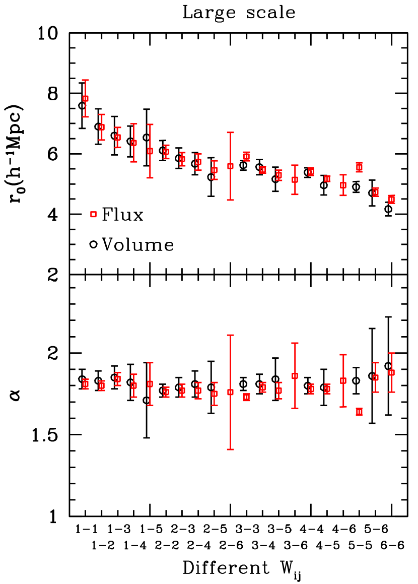
Figure 3.— The correlation length, $r_{0}$, and logarithmic slope, $\alpha$, obtained from the projected auto- and cross-correlation functions on scales $0.98\>h^{-1}{\rm{Mpc}}\leq r_{p}\leq 9.6\>h^{-1}{\rm{Mpc}}$ for various volume-limited and flux-limited samples. The error-bars are 1-$\sigma$ scatter among the three SDSS regions. In the horizontal axis we indicate the IDs ($i-j$) of the samples used in the estimate of the correlation function, $W_{i,j}$. The circles with error-bars are the results for volume-limited samples. The squares with error-bars are the results for flux-limited samples. Note that since the overlap region is too small, we do not have measurement of 1-6, 2-6, 3-6 and 4-6 data points for volume-limited samples and 1-6 for flux-limited samples. Overall, the results for volume-limited and flux-limited samples agree well. Large discrepancy exists for $W_{5,5}$, likely due to the existence of the supercluster at redshift $z\sim 0.08$.

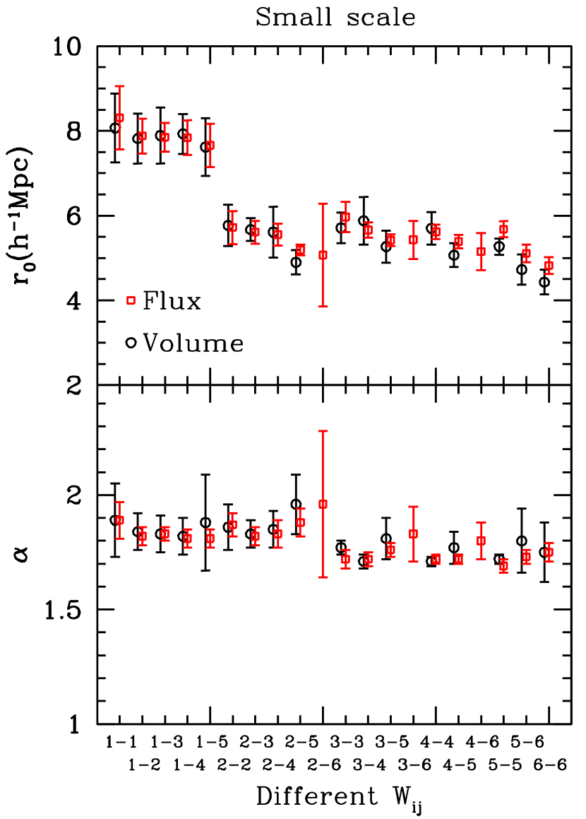
Figure 4.— The same as Fig. 3 except that the results are obtained from the fitting to the correlation functions on small scales ($0.16\>h^{-1}{\rm{Mpc}}\leq r_{p}\leq 0.98\>h^{-1}{\rm{Mpc}}$). Note again that since the overlap region is too small, we do not have measurement of 1-6, 2-6, 3-6 and 4-6 data points for volume-limited samples and 1-6 for flux-limited samples.

Table 3The correlation lengths and slopes for volume-limited samples on large scales ($0.98\>h^{-1}{\rm{Mpc}}\leq r_{p}\leq 9.6\>h^{-1}{\rm{Mpc}}$) .

Sample	Va	Vb	Vc	Vd	Ve	Vf
	$\alpha$	$\alpha$	$\alpha$	$\alpha$	$\alpha$	$\alpha$
	$r_{0}$	$r_{0}$	$r_{0}$	$r_{0}$	$r_{0}$	$r_{0}$
V1	$1.84\pm 0.06$
	$7.59\pm 0.75$
V2	$1.83\pm 0.06$	$1.77\pm 0.04$
	$6.90\pm 0.59$	$6.11\pm 0.33$
V3	$1.85\pm 0.07$	$1.79\pm 0.06$	$1.81\pm 0.04$
	$6.60\pm 0.64$	$5.85\pm 0.34$	$5.62\pm 0.16$
V4	$1.82\pm 0.11$	$1.81\pm 0.08$	$1.81\pm 0.06$	$1.80\pm 0.05$
	$6.41\pm 0.51$	$5.67\pm 0.37$	$5.56\pm 0.25$	$5.38\pm 0.16$
V5	$1.71\pm 0.23$	$1.79\pm 0.16$	$1.84\pm 0.13$	$1.79\pm 0.11$	$1.83\pm 0.08$
	$6.54\pm 0.94$	$5.23\pm 0.64$	$5.16\pm 0.40$	$4.96\pm 0.32$	$4.90\pm 0.18$
V6					$1.86\pm 0.29$	$1.92\pm 0.30$
					$4.70\pm 0.43$	$4.17\pm 0.23$
$\alpha=\overline{\alpha}=1.82$	$r_{0}$	$r_{0}$	$r_{0}$	$r_{0}$	$r_{0}$	$r_{0}$
V1	$7.57\pm 0.45$
V2	$6.89\pm 0.34$	$6.13\pm 0.18$
V3	$6.56\pm 0.38$	$5.87\pm 0.20$	$5.62\pm 0.11$
V4	$6.40\pm 0.39$	$5.67\pm 0.23$	$5.56\pm 0.14$	$5.39\pm 0.11$
V5	$6.56\pm 0.58$	$5.26\pm 0.37$	$5.14\pm 0.29$	$4.97\pm 0.21$	$4.89\pm 0.09$
V6					$4.65\pm 0.38$	$4.08\pm 0.20$

Note. — The upper part lists the best fit values of $r_{0}$ and $\alpha$ for different volume-limited samples, using data points on large scales, $0.98\>h^{-1}{\rm{Mpc}}\leq r_{p}\leq 9.6\>h^{-1}{\rm{Mpc}}$. The table is not filled up because the overlaps in volume between the faintest and bright samples are too small to allow reliable estimates of the cross correlation functions. The lower part of the table shows the correlation length obtained by setting the slope of the correlation functions, $\alpha$, to be $\overline{\alpha}=1.82$, the average of the values listed in the upper part.

Table 4The correlation lengths and slopes for volume-limited samples on small scales ($0.16\>h^{-1}{\rm{Mpc}}\leq r_{p}\leq 0.98\>h^{-1}{\rm{Mpc}}$)

Sample	Va	Vb	Vc	Vd	Ve	Vf
	$\alpha$	$\alpha$	$\alpha$	$\alpha$	$\alpha$	$\alpha$
	$r_{0}$	$r_{0}$	$r_{0}$	$r_{0}$	$r_{0}$	$r_{0}$
V1	$1.89\pm 0.16$
	$8.07\pm 0.81$
V2	$1.84\pm 0.08$	$1.86\pm 0.10$
	$7.82\pm 0.59$	$5.77\pm 0.49$
V3	$1.83\pm 0.08$	$1.83\pm 0.06$	$1.77\pm 0.03$
	$7.89\pm 0.66$	$5.67\pm 0.27$	$5.71\pm 0.36$
V4	$1.82\pm 0.08$	$1.85\pm 0.08$	$1.71\pm 0.03$	$1.71\pm 0.02$
	$7.93\pm 0.47$	$5.61\pm 0.60$	$5.88\pm 0.56$	$5.70\pm 0.38$
V5	$1.88\pm 0.21$	$1.96\pm 0.13$	$1.81\pm 0.09$	$1.77\pm 0.07$	$1.72\pm 0.02$
	$7.62\pm 0.68$	$4.90\pm 0.29$	$5.27\pm 0.38$	$5.07\pm 0.28$	$5.27\pm 0.19$
V6					$1.80\pm 0.14$	$1.75\pm 0.13$
					$4.73\pm 0.36$	$4.43\pm 0.29$
$\alpha=\overline{\alpha}=1.81$	$r_{0}$	$r_{0}$	$r_{0}$	$r_{0}$	$r_{0}$	$r_{0}$
V1	$8.16\pm 0.54$
V2	$7.21\pm 0.40$	$6.00\pm 0.13$
V3	$7.07\pm 0.36$	$5.74\pm 0.12$	$5.53\pm 0.09$
V4	$6.99\pm 0.46$	$5.76\pm 0.13$	$5.44\pm 0.08$	$5.27\pm 0.06$
V5	$6.70\pm 0.26$	$5.45\pm 0.23$	$5.25\pm 0.12$	$4.93\pm 0.09$	$4.90\pm 0.11$
V6					$4.69\pm 0.14$	$4.23\pm 0.09$

Note. — The same as Table 3, except that the results are obtained by fitting the correlation functions on small scales, $0.16\>h^{-1}{\rm{Mpc}}\leq r_{p}\leq 0.98\>h^{-1}{\rm{Mpc}}$.

We estimate both the 2-point auto- and cross-correlation functions (hereafter 2PCFs) using the definition proposed in Davis & Peebles (1983),

$$\xi_{i,j}(r_{p},r_{\pi})={D_{i}D_{j}(r_{p},r_{\pi})\over D_{i}R_{j}(r_{p},r_{\pi})}-1\,,$$ (3)

where $i,j$ denote the pair of samples for which the cross correlation function is estimated; $i=j$ corresponds to auto-correlation function. As a convention, sample $i$ always represents the brighter sample if $i\neq j$. In the above definition, $D_{i}D_{j}$ is the count of galaxy pairs between samples $i$ and $j$, $D_{i}R_{j}$ is the count of galaxy-random pairs between galaxy sample $i$ and random sample $j$, and $r_{p}$ and $r_{\pi}$ are the separations of galaxy pairs perpendicular and parallel to the line of sight, respectively. Galaxy-galaxy and galaxy-random pairs are counted in logarithmic bins in $r_{p}$, with bin width $\Delta\log_{10}(r_{p})=0.2$, and in linear bins of $r_{\pi}$, with bin width $\Delta r_{\pi}=1\>h^{-1}{\rm{Mpc}}$. Since we have galaxy samples in three different regions (NGCE, NGCO and SGC), we combine the number counts of all regions when estimating the correlation function. The scatter among the three regions are used to indicate the uncertainties (error-bars) in the measurements. Note that the errors of the 2PCFs for the faintest sample may be somewhat underestimated compared to the true cosmic variance because the volumes and separations of these three regions are too small to represent the true cosmic variance.

As mentioned in Section 2.1, the redshift overlap between some of the volume-limited samples is very small, especially between the bright and faint samples. In fact, samples V1 and V5 as well as V1 and V6 have no overlap-volume at all (cf. Fig.1). In those cases we have to use samples Va – Vf (which may be incomplete) to get better statistics. According to Eq. (3), one may circumvent the problems to some extent using combinations of complete and incomplete samples. For example, one can choose the $i$ sample from Va - Vf, and the $j$ sample and the corresponding random sample from V1 - V6. Since V1 - V6 are complete, this reduces the effects due to the incompleteness in samples Va – Vf.

In our following discussion, we will focus on the projected 2PCF, which is defined as

$$W_{i,j}(r_{p})=2\int_{0}^{\infty}\xi_{i,j}(r_{p},r_{\pi})dr_{\pi}=2\sum_{k}\xi_{i,j}(r_{p},r_{\pi,k})\Delta r_{\pi,k}\,.$$ (4)

Here the summation is made over $k=1$ to 40 corresponding to $r_{\pi}=0.5\>h^{-1}{\rm{Mpc}}$ to $r_{\pi}=39.5\>h^{-1}{\rm{Mpc}}$. If we assume that the real-space 2PCF $\xi(r)$ can be fitted by a power law,

$$\xi(r)=(r_{0}/r)^{\alpha}\,,$$ (5)

where $r_{0}$ and $\alpha$ are, respectively, the correlation length and slope of the correlation function, then the projected 2PCF is related to the real-space 2PCF as

$$W(r_{p})=r_{0}^{\alpha}r_{p}^{1-\alpha}\frac{\Gamma(1/2)\Gamma[(\alpha-1)/2]}{\Gamma(\alpha/2)}\,,$$ (6)

where $\Gamma(x)$ is the Gamma function. As we will see below, the observed 2PCFs can all be fitted reasonably well by power laws over limited ranges of $r_{p}$. We can then use $r_{0}$ to represent the correlation amplitude, and $\alpha$ the shape of the correlation function.

4. Dependence on galaxy luminosity

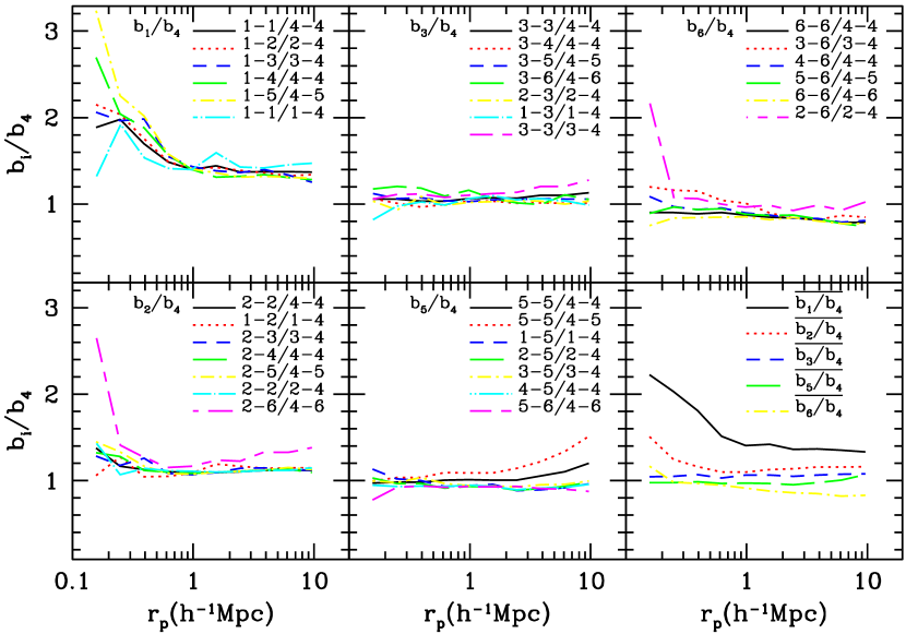
Figure 5.— The relative bias as a function of $r_{p}$ obtained from the ratios of the projected correlation functions of the flux-limited samples. In the lower-right panel, we show the mean relative bias parameters obtained by averaging the results shown in each of the five panels. In each panel, $i-j$ means that the projected two-point correlation function is for samples Fi and Fj.

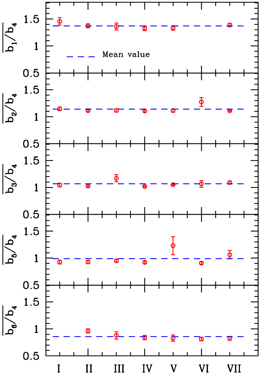
Figure 6.— The relative bias parameters obtained from the correlation functions over $0.98\>h^{-1}{\rm{Mpc}}$ to $9.8\>h^{-1}{\rm{Mpc}}$ using seven different approaches (see the main text for details). The error-bars are based on the scatter of the data points in the range $0.98\>h^{-1}{\rm{Mpc}}<r_{p}\leq 9.8\>h^{-1}{\rm{Mpc}}$. Panels from top to bottom correspond to the bias parameters for Fi ($i=1,2,3,5,6$), normalized by that of F4. The horizontal axis labels the different approaches that are used to determine the bias parameter for each subsample. One data point is missing in the first and fifth panels, because the redshift overlap between F1 and F6 is too small to measure the cross-correlation function reliably.

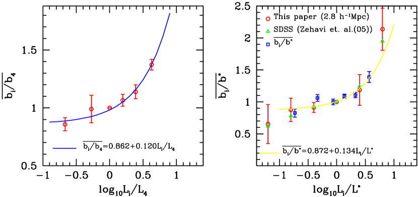
Figure 7.— Left panel: The average relative bias parameter, obtained using the correlation data in $0.98\>h^{-1}{\rm{Mpc}}<r_{p}\leq 9.8\>h^{-1}{\rm{Mpc}}$ as a function of galaxy luminosity. The results are obtained using the flux-limited samples, and both the bias parameter and the luminosity are normalized by the values for F4. For a given luminosity, the mean and error-bar are based on the different measurements shown in Fig 6. The solid curve shows the relation, $\overline{b_{i}/b_{4}}=0.862+0.120L_{i}/L_{4}$, obtained by fitting the data. Right panel: In this panel, we compare our results with those obtained by Zehavi et al. (2005). Here the bias parameters and the luminosities are normalized by the values for $L^{*}$ galaxies. In Zehavi et al., the relative bias parameters are measured using the auto-correlation functions at $r_{p}=2.7\>h^{-1}{\rm{Mpc}}$ for six volume-limited samples with luminosities in $(-23.0,-22.0)$, $(-22.0,-21.0)$, $(-21.0,-20.0)$, $(-20.0,-19.0)$, $(-19.0,-18.0)$, $(-18.0,-17.0)$, and their results are shown by triangles. Using the same method and same samples, our results (however at $r_{p}=2.8\>h^{-1}{\rm{Mpc}}$) are shown as open circles and match very well their results. The open squares show the same results as shown in the left panel, except that the normalizations are different. The curve is a fit to the results represented by the open squares.

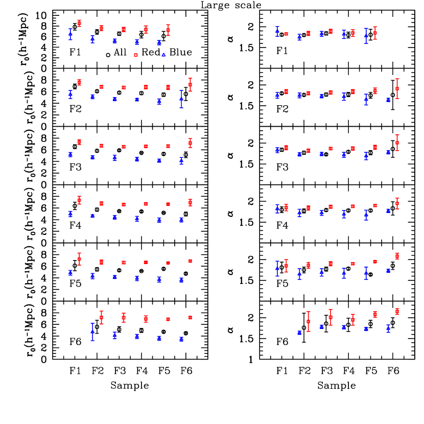
Figure 8.— Here we compare the correlation lengths ($r_{0}$) and slopes ($\alpha$) of all (circles), red (squares) and blue (triangles) galaxies using flux-limited samples (F1 – F6 for all galaxies; $\rm F1_{red}$ – $\rm F6_{red}$ for red galaxies, and $\rm F1_{blue}$ – $\rm F6_{blue}$ for blue galaxies). Here the results are based on correlation functions on large scales, $0.98\>h^{-1}{\rm{Mpc}}\leq r_{p}\leq 9.6\>h^{-1}{\rm{Mpc}}$. To avoid confusion, data points for rad and blue galaxies are shifted slightly horizontally.

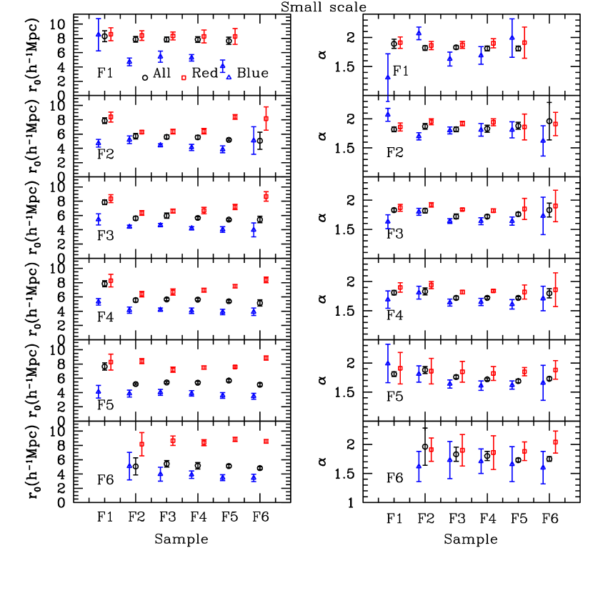
Figure 9.— The same as Fig. 8, except that the results are based on the correlation functions on small scales, $0.16\>h^{-1}{\rm{Mpc}}\leq r_{p}\leq 0.98\>h^{-1}{\rm{Mpc}}$.

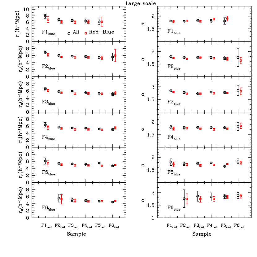
Figure 10.— The correlation lengths ($r_{0}$) and slopes ($\alpha$) of the cross-correlation functions between red and blue galaxies (squares) on large scales, $0.98\>h^{-1}{\rm{Mpc}}\leq r_{p}\leq 9.6\>h^{-1}{\rm{Mpc}}$. Panels from top to bottom correspond to flux limited samples for blue galaxies ${\rm Fi_{blue}}$ ($i=1,2...,6$). The red samples used in the cross-correlations are labeled on the horizontal axis ${\rm Fi_{red}}$ ($i=1,2...,6$). For comparison, results for all galaxies in the corresponding flux-limited samples are plotted as open circles.

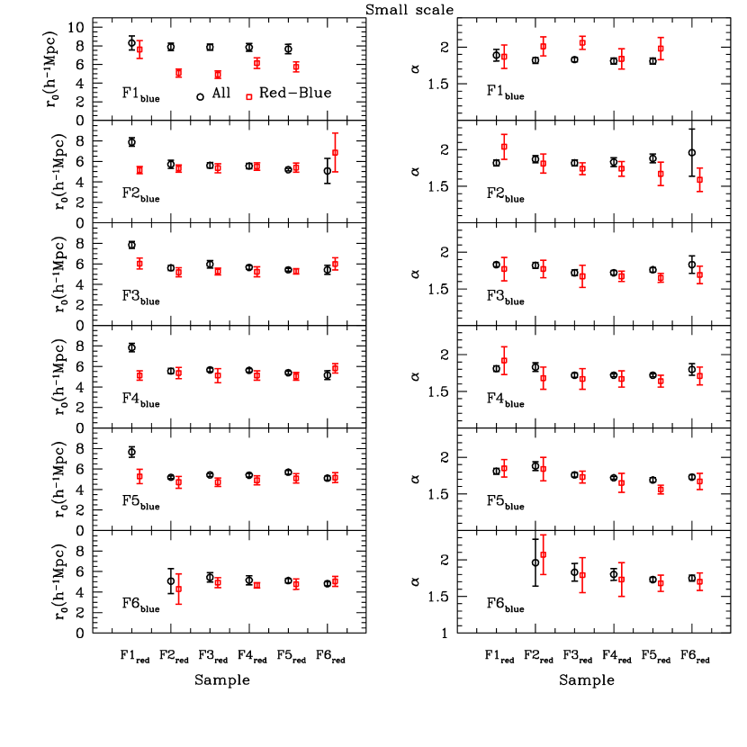
Figure 11.— The same as Fig. 10, but here results are based on correlation functions on small scales, $0.16\>h^{-1}{\rm{Mpc}}\leq r_{p}\leq 0.98\>h^{-1}{\rm{Mpc}}$.

Table 5The correlation lengths and slopes for flux-limited samples on large scales ($0.98\>h^{-1}{\rm{Mpc}}\leq r_{p}\leq 9.6\>h^{-1}{\rm{Mpc}}$)

Sample	F1	F2	F3	F4	F5	F6
	$\alpha$	$\alpha$	$\alpha$	$\alpha$	$\alpha$	$\alpha$
	$r_{0}$	$r_{0}$	$r_{0}$	$r_{0}$	$r_{0}$	$r_{0}$
F1	$1.81\pm 0.03$
	$7.83\pm 0.61$
F2	$1.80\pm 0.03$	$1.76\pm 0.03$
	$6.88\pm 0.42$	$6.06\pm 0.22$
F3	$1.84\pm 0.04$	$1.77\pm 0.04$	$1.73\pm 0.02$
	$6.54\pm 0.33$	$5.82\pm 0.22$	$5.91\pm 0.14$
F4	$1.80\pm 0.07$	$1.77\pm 0.05$	$1.79\pm 0.03$	$1.78\pm 0.03$
	$6.36\pm 0.63$	$5.73\pm 0.27$	$5.47\pm 0.11$	$5.41\pm 0.13$
F5	$1.81\pm 0.13$	$1.75\pm 0.07$	$1.77\pm 0.05$	$1.78\pm 0.03$	$1.64\pm 0.02$
	$6.09\pm 0.88$	$5.46\pm 0.31$	$5.29\pm 0.17$	$5.17\pm 0.09$	$5.55\pm 0.15$
F6		$1.76\pm 0.35$	$1.86\pm 0.20$	$1.83\pm 0.16$	$1.85\pm 0.09$	$1.88\pm 0.12$
		$5.59\pm 1.12$	$5.14\pm 0.48$	$4.96\pm 0.34$	$4.73\pm 0.14$	$4.49\pm 0.13$
$\alpha=\overline{\alpha}=1.79$	$r_{0}$	$r_{0}$	$r_{0}$	$r_{0}$	$r_{0}$	$r_{0}$
F1	$7.80\pm 0.31$
F2	$6.86\pm 0.21$	$6.09\pm 0.13$
F3	$6.49\pm 0.19$	$5.83\pm 0.12$	$5.94\pm 0.14$
F4	$6.34\pm 0.35$	$5.75\pm 0.18$	$5.48\pm 0.15$	$5.42\pm 0.14$
F5	$6.07\pm 0.56$	$5.48\pm 0.29$	$5.31\pm 0.10$	$5.17\pm 0.09$	$5.65\pm 0.11$
F6		$5.62\pm 0.46$	$5.08\pm 0.37$	$4.93\pm 0.21$	$4.68\pm 0.11$	$4.38\pm 0.12$

Table 6The correlation lengths and slopes for flux-limited samples on small scales ($0.16\>h^{-1}{\rm{Mpc}}\leq r_{p}\leq 0.98\>h^{-1}{\rm{Mpc}}$)

Sample	F1	F2	F3	F4	F5	F6
	$\alpha$	$\alpha$	$\alpha$	$\alpha$	$\alpha$	$\alpha$
	$r_{0}$	$r_{0}$	$r_{0}$	$r_{0}$	$r_{0}$	$r_{0}$
F1	$1.89\pm 0.08$
	$8.31\pm 0.75$
F2	$1.82\pm 0.04$	$1.87\pm 0.05$
	$7.88\pm 0.41$	$5.72\pm 0.39$
F3	$1.83\pm 0.03$	$1.82\pm 0.04$	$1.72\pm 0.04$
	$7.85\pm 0.34$	$5.61\pm 0.27$	$5.97\pm 0.36$
F4	$1.81\pm 0.04$	$1.83\pm 0.06$	$1.72\pm 0.03$	$1.72\pm 0.02$
	$7.84\pm 0.41$	$5.55\pm 0.26$	$5.66\pm 0.18$	$5.62\pm 0.17$
F5	$1.81\pm 0.04$	$1.88\pm 0.06$	$1.76\pm 0.03$	$1.72\pm 0.02$	$1.69\pm 0.03$
	$7.66\pm 0.51$	$5.19\pm 0.13$	$5.42\pm 0.14$	$5.39\pm 0.16$	$5.68\pm 0.19$
F6		$1.96\pm 0.32$	$1.83\pm 0.12$	$1.80\pm 0.08$	$1.73\pm 0.03$	$1.75\pm 0.04$
		$5.07\pm 1.21$	$5.43\pm 0.45$	$5.15\pm 0.44$	$5.11\pm 0.21$	$4.82\pm 0.20$
$\alpha=\overline{\alpha}=1.80$	$r_{0}$	$r_{0}$	$r_{0}$	$r_{0}$	$r_{0}$	$r_{0}$
F1	$8.21\pm 0.42$
F2	$7.17\pm 0.23$	$6.01\pm 0.19$
F3	$6.93\pm 0.11$	$5.71\pm 0.19$	$5.61\pm 0.15$
F4	$6.96\pm 0.13$	$5.69\pm 0.18$	$5.33\pm 0.06$	$5.29\pm 0.15$
F5	$6.77\pm 0.16$	$5.50\pm 0.15$	$5.25\pm 0.17$	$5.10\pm 0.18$	$5.24\pm 0.14$
F6		$5.69\pm 0.59$	$5.54\pm 0.09$	$5.13\pm 0.13$	$4.85\pm 0.17$	$4.64\pm 0.15$

Table 7The correlation lengths and slopes for flux-limited samples of red galaxies on large scales ($0.98\>h^{-1}{\rm{Mpc}}\leq r_{p}\leq 9.6\>h^{-1}{\rm{Mpc}}$)

Sample	${\rm F1_{red}}$	${\rm F2_{red}}$	${\rm F3_{red}}$	${\rm F4_{red}}$	${\rm F5_{red}}$	${\rm F6_{red}}$
	$\alpha$	$\alpha$	$\alpha$	$\alpha$	$\alpha$	$\alpha$
	$r_{0}$	$r_{0}$	$r_{0}$	$r_{0}$	$r_{0}$	$r_{0}$
${\rm F1_{red}}$	$1.83\pm 0.03$
	$8.50\pm 0.59$
${\rm F2_{red}}$	$1.84\pm 0.05$	$1.80\pm 0.04$
	$7.59\pm 0.48$	$6.82\pm 0.26$
${\rm F3_{red}}$	$1.89\pm 0.05$	$1.82\pm 0.04$	$1.87\pm 0.03$
	$7.33\pm 0.41$	$6.70\pm 0.24$	$6.53\pm 0.20$
${\rm F4_{red}}$	$1.85\pm 0.08$	$1.84\pm 0.05$	$1.87\pm 0.04$	$1.88\pm 0.03$
	$7.34\pm 0.68$	$6.78\pm 0.30$	$6.59\pm 0.18$	$6.71\pm 0.18$
${\rm F5_{red}}$	$1.85\pm 0.15$	$1.86\pm 0.07$	$1.90\pm 0.05$	$1.90\pm 0.03$	$1.95\pm 0.02$
	$7.23\pm 1.03$	$6.71\pm 0.36$	$6.63\pm 0.24$	$6.66\pm 0.12$	$6.55\pm 0.11$
${\rm F6_{red}}$		$1.91\pm 0.24$	$2.01\pm 0.19$	$1.95\pm 0.13$	$2.08\pm 0.07$	$2.15\pm 0.07$
		$7.19\pm 1.11$	$7.16\pm 0.78$	$6.93\pm 0.56$	$6.89\pm 0.18$	$7.18\pm 0.18$
$\alpha=\overline{\alpha}=1.90$	$r_{0}$	$r_{0}$	$r_{0}$	$r_{0}$	$r_{0}$	$r_{0}$
${\rm F1_{red}}$	$8.50\pm 0.44$
${\rm F2_{red}}$	$7.60\pm 0.36$	$6.82\pm 0.25$
${\rm F3_{red}}$	$7.33\pm 0.35$	$6.71\pm 0.25$	$6.52\pm 0.13$
${\rm F4_{red}}$	$7.35\pm 0.37$	$6.77\pm 0.34$	$6.59\pm 0.21$	$6.70\pm 0.14$
${\rm F5_{red}}$	$7.24\pm 0.32$	$6.70\pm 0.33$	$6.62\pm 0.23$	$6.66\pm 0.12$	$6.56\pm 0.09$
${\rm F6_{red}}$		$7.19\pm 0.78$	$7.17\pm 0.19$	$6.92\pm 0.22$	$6.97\pm 0.29$	$7.25\pm 0.31$

Table 8The correlation lengths and slopes for flux-limited samples of red galaxies on small scales ($0.16\>h^{-1}{\rm{Mpc}}\leq r_{p}\leq 0.98\>h^{-1}{\rm{Mpc}}$)

Sample	${\rm F1_{red}}$	${\rm F2_{red}}$	${\rm F3_{red}}$	${\rm F4_{red}}$	${\rm F5_{red}}$	${\rm F6_{red}}$
	$\alpha$	$\alpha$	$\alpha$	$\alpha$	$\alpha$	$\alpha$
	$r_{0}$	$r_{0}$	$r_{0}$	$r_{0}$	$r_{0}$	$r_{0}$
${\rm F1_{red}}$	$1.91\pm 0.10$
	$8.59\pm 0.90$
${\rm F2_{red}}$	$1.86\pm 0.07$	$1.95\pm 0.05$
	$8.40\pm 0.69$	$6.28\pm 0.23$
${\rm F3_{red}}$	$1.87\pm 0.06$	$1.92\pm 0.04$	$1.84\pm 0.02$
	$8.35\pm 0.55$	$6.36\pm 0.34$	$6.62\pm 0.28$
${\rm F4_{red}}$	$1.90\pm 0.08$	$1.94\pm 0.06$	$1.82\pm 0.03$	$1.84\pm 0.02$
	$8.27\pm 0.89$	$6.40\pm 0.38$	$6.69\pm 0.44$	$6.94\pm 0.27$
${\rm F5_{red}}$	$1.91\pm 0.27$	$1.86\pm 0.22$	$1.85\pm 0.18$	$1.82\pm 0.12$	$1.85\pm 0.07$
	$8.28\pm 1.12$	$8.40\pm 0.34$	$7.20\pm 0.36$	$7.50\pm 0.24$	$7.59\pm 0.16$
${\rm F6_{red}}$		$1.91\pm 0.20$	$1.90\pm 0.27$	$1.86\pm 0.29$	$1.88\pm 0.16$	$2.04\pm 0.19$
		$8.17\pm 1.64$	$8.66\pm 0.66$	$8.39\pm 0.41$	$8.85\pm 0.29$	$8.58\pm 0.26$
$\alpha=\overline{\alpha}=1.89$	$r_{0}$	$r_{0}$	$r_{0}$	$r_{0}$	$r_{0}$	$r_{0}$
${\rm F1_{red}}$	$8.52\pm 0.49$
${\rm F2_{red}}$	$7.62\pm 0.43$	$6.61\pm 0.18$
${\rm F3_{red}}$	$7.75\pm 0.33$	$6.54\pm 0.14$	$6.42\pm 0.31$
${\rm F4_{red}}$	$8.04\pm 0.23$	$6.72\pm 0.16$	$6.59\pm 0.33$	$6.76\pm 0.26$
${\rm F5_{red}}$	$8.13\pm 0.49$	$7.03\pm 0.18$	$6.97\pm 0.16$	$7.00\pm 0.24$	$7.33\pm 0.15$
${\rm F6_{red}}$		$7.63\pm 0.83$	$8.78\pm 0.36$	$8.04\pm 0.34$	$8.64\pm 0.22$	$10.12\pm 0.25$

We start our investigation by comparing the projected 2PCFs obtained using the volume-limited and flux-limited samples. When calculating the projected 2PCFs with the volume-limited samples, we use combinations of the set V1–V6 with the set Va–Vf for the reasons given in Section  3. Since the results are very similar for the volume-limited and the flux-limited samples, we show only the results for the flux-limited samples in Fig. 2, where we compare the projected 2PCFs based on random samples of type R1 with those based on random samples of type R2. As found by Li et al. (2006), the two types of random samples give almost identical results in most cases. The largest discrepancy is seen in the auto 2PCF of sample F5, This sample is significantly affected by the supercluter at redshift $z\sim 0.08$, and the points in sample R1 is not completely random due to the way it is constructed. Since overall the random samples of type R1 work quite well and since their construction does not require the luminosity function of galaxies, the results presented below will be based on this type of random samples. A comparison of the various projected 2PCFs in Fig. 2 shows that brighter galaxies are on average more strongly clustered, an effect that we will describe in more detail in the following.

To quantify the observed 2PCFs, we fit to the projected 2PCFs according to Eq. (6) with the two free parameters $r_{0}$ and $\alpha$. A larger value of $r_{0}$ implies a stronger clustering strength, while a larger $\alpha$ implies a steeper correlation function. In order to see how $r_{0}$ and $\alpha$ might change with scales, we fit the projected 2PCFs separately over two scale ranges, $0.98\>h^{-1}{\rm{Mpc}}\leq r_{p}\leq 9.6\>h^{-1}{\rm{Mpc}}$ and $0.16\>h^{-1}{\rm{Mpc}}\leq r_{p}\leq 0.98\>h^{-1}{\rm{Mpc}}$. The separation between large and small scales is made at $r_{p}\sim 1\>h^{-1}{\rm{Mpc}}$, because the correlation function on smaller scales is expected to be dominated by the one-halo term, while that on larger scales by the two-halo term, as shown in Yang et al. (2005). We use two methods to obtain $r_{0}$ and $\alpha$ from the data. In the first method, we obtain $r_{0}$ and $\alpha$ directly from the fit to the projected 2PCFs. In the second one, we first obtain an average value of $\alpha$, ${\overline{\alpha}}$, from all the correlation functions and then fit the projected 2PCF to get $r_{0}$ keeping $\alpha={\overline{\alpha}}$. The fitting parameters so obtained are listed in Tables 3, 4, 5 and 6, separately for volume-limited and flux-limited samples, and for large and small scales.

Fig. 3 compares the values of $r_{0}$ and $\alpha$ on large scales ($0.98\>h^{-1}{\rm{Mpc}}\leq r_{p}\leq 9.6\>h^{-1}{\rm{Mpc}}$) obtained from the volume-limited samples with those obtained from the corresponding flux-limited samples. Overall, the results for these two kinds of samples are similar. The only exception is $W_{5,5}$, where the values of $r_{0}$ and $\alpha$ for the volume-limited and flux-limited samples are significantly different, largely because the presence of the supercluster at $z\sim 0.08$ that makes the correlation properties quite sensitive to how the sample is exactly formed. There is a clear trend in the correlation length $r_{0}$ that brighter galaxies have larger $r_{0}$. The cross-correlations between bright and faint galaxies are also stronger than the auto correlations of faint galaxies. On the other hand the slope of the correlation function does not show any strong trend with luminosity, and the mean value of and scatter in $\alpha$ are $1.82\pm 0.04$ for the volume-limited samples and $1.79\pm 0.05$ for the flux-limited samples. The correlation lengths obtained by fixing $\alpha$ at these mean values are also listed in Tables  3, 4, 5 and 6 for comparison.

In order to investigate how the clustering strengths change on small scales, we fit the projected 2PCFs with power laws in the range $0.16\>h^{-1}{\rm{Mpc}}\leq r_{p}\leq 0.98\>h^{-1}{\rm{Mpc}}$, and the results are shown in Fig. 4 and listed in Tables 4 and 6. A comparison to the results shown in Fig. 3 shows that the clustering strengths for the samples that involve the brightest galaxies are enhanced on small scales; in particular the cross correlation between the brightest and faintest galaxies is much stronger on small scales. For faint galaxies, the clustering strengths on small scales are similar to those based on the power laws obtained on large scales. This suggests that there is a significant population of faint galaxies that are distributed around the brightest galaxies and the number drops rapidly with the increase of the distance to the brightest galaxies. As we will see below, it is likely that this population is dominated by faint red galaxies in clusters and groups.

Having investigated the clustering strengths for galaxies of different luminosities, we now study the bias factor in the distribution of galaxies as a function of galaxy luminosity. Since we do not know the two-point correlation function of the cosmic density field, we can only study the bias factor in a relative sense. To do this, we choose F4 as our fiducial sample, because it has a good overlap in volume with both the faint and bright samples. Since each sample is used in a number of projected 2PCFs, we can estimate the relative bias for each sample in a number of ways. With F4 as the reference sample, the bias factor for the $i$th sample can be estimated from one of the following definitions:

$$\frac{b_{i}}{b_{4}} = \frac{W_{i,j}}{W_{j,4}}(j=1,2,3,4,5,6)\,,$$ (7)

$$\frac{b_{i}}{b_{4}} = \sqrt{\frac{W_{i,i}}{W_{4,4}}}\,,$$

where $i=1,2,3,5,6$. Thus, each relative bias can be estimated using seven different approaches. In what follows, these seven approaches will be referred as approaches I, II, $\cdot\cdot\cdot$, VI, corresponding to $j=1,2,\cdot\cdot\cdot,6$, respectively, and approach VII, corresponding to the definition in the second line of equation (7). Note that in general the relative bias factors, $b_{i}/b_{4}$, obtained from different approaches are not expected to be the same. As we will discuss in Section 6, these relative bias factors are expected to be the same only under the assumption that the bias for galaxies of different luminosities is linear and that the stochastic component in the bias relations between different galaxies is small.

The first 5 panels in Fig. 5 show the relative bias factor as a function of $r_{p}$ for the five samples, Fi ($i=1,2,3,5,6$), and the 7 different lines within each panel show the results obtained using the 7 different approaches described above. For most cases, the bias function is almost independent of $r_{p}$ at $r_{p}>1\>h^{-1}{\rm{Mpc}}$, indicating that nonlinearity in the relative bias is small on these scales. The bias factors obtained using the 7 different approaches agree quite well with each other. Their averages are shown in the lower-right panel which clearly shows that brighter galaxies have higher relative biases.

To quantify the relative bias as a function of luminosity, we estimate a mean relative bias factor for each case by averaging the bias function over $1\>h^{-1}{\rm{Mpc}}$-$10\>h^{-1}{\rm{Mpc}}$. The results are shown in Fig. 6 for different luminosity samples using the 7 approaches. Note that there is one data point missing in the first and fifth panels, because the overlap between samples F1 and F6 is too small to have a reliable measurement of $W_{1,6}$. The dashed line in each panel is the average value of the relative bias obtained from the seven different approaches. As one can see, the relative bias factors obtained with different approaches are consistent with each other. We estimate the mean luminosity of galaxies in each sample F1–F6 as $L_{i}$, and the corresponding average absolute magnitudes thus obtained are $-21.87$, $-21.24$, $-20.76$, $-20.27$, $-19.61$, and $-18.62$, respectively. These magnitudes are then converted into luminosities to represent the characteristic luminosities of the samples in question. The left panel of Fig. 7 shows the average relative bias factor versus $L_{i}/L_{4}$ as open circles, with error-bars representing the scatter among the seven different approaches. There is a clear trend that the relative bias increases with galaxy luminosity. The solid curve is a linear fit to the data: $\overline{b_{i}/b_{4}}=0.862+0.120L_{i}/L_{4}$.

The luminosity dependence of galaxy bias in the SDSS has been investigated by Zehavi et al. (2005) using the amplitudes of the auto correlation functions at a fixed projected radius $r_{p}=2.7\>h^{-1}{\rm{Mpc}}$ obtained from six volume-limited samples with $M_{r}$ in $(-23,-22)$, $(-22,-21)$, $(-21,-20)$, $(-20,-19)$, $(-19,-18)$, $(-18,-17)$. The bias factors were normalized relative to $L^{*}$ galaxies defined to be the ones with $M_{r}$ in $(-21,-20)$. To compare our results with theirs, we show in the right panel of Fig. 7 the relative bias factors obtained by Zehavi et al. as triangles together with our results (open circles) that are obtained from the auto-correlation amplitudes at a fixed, but a slightly different, projected radius $r_{p}=2.8\>h^{-1}{\rm{Mpc}}$. Note that our results are in excellent agreement with the results obtained by Zehavi et al. (2005). For the relative bias - luminosity relation shown in the left panel of Fig. 7, we can convert it into a relation with $L/L^{*}$. The characteristic luminosity for sample F* is $-20.47$, very close to $L^{*}$. Using the projected 2PCF for F*, $W_{\star,\star}$, we can write

$$\overline{b_{i}/b^{*}}=\overline{b_{i}/b_{4}\sqrt{\frac{W_{4,4}}{W_{*,*}}}}\,,$$ (8)

where $W_{4,4}$ and $W_{*,*}$ are the projected auto 2PCFs of samples F4 and F*, respectively. We first calculate $b_{i}/b^{*}$ at different scales and then average these biases over $1\>h^{-1}{\rm{Mpc}}$-$10\>h^{-1}{\rm{Mpc}}$ to obtain the average bias $\overline{b_{i}/b^{*}}$. The resulting $\overline{b_{i}/b^{*}}$ - $L/L_{\star}$ relation is shown by the open squares in the right panel of Fig. 7. Fitted with a linear model, this relation can be described as $\overline{b_{i}/b^{*}}=0.872+0.134L_{i}/L^{*}$. As one can see, our results based on the cross-correlation match well those of Zehavi et al. (2005). The implications of this agreement will be discussed in Section 6.

5. Dependence on galaxy color

Table 9The correlation length and slope for flux-limited samples of blue galaxies on large scales ($0.98\>h^{-1}{\rm{Mpc}}\leq r_{p}\leq 9.6\>h^{-1}{\rm{Mpc}}$)

Sample	${\rm F1_{blue}}$	${\rm F2_{blue}}$	${\rm F3_{blue}}$	${\rm F4_{blue}}$	${\rm F5_{blue}}$	${\rm F6_{blue}}$
	$\alpha$	$\alpha$	$\alpha$	$\alpha$	$\alpha$	$\alpha$
	$r_{0}$	$r_{0}$	$r_{0}$	$r_{0}$	$r_{0}$	$r_{0}$
${\rm F1_{blue}}$	$1.89\pm 0.12$
	$6.45\pm 1.03$
${\rm F2_{blue}}$	$1.75\pm 0.07$	$1.75\pm 0.06$
	$5.50\pm 0.69$	$5.11\pm 0.33$
${\rm F3_{blue}}$	$1.83\pm 0.06$	$1.73\pm 0.04$	$1.74\pm 0.04$
	$5.17\pm 0.36$	$4.71\pm 0.27$	$4.63\pm 0.46$
${\rm F4_{blue}}$	$1.82\pm 0.10$	$1.72\pm 0.09$	$1.72\pm 0.06$	$1.69\pm 0.09$
	$4.97\pm 0.45$	$4.62\pm 0.21$	$4.39\pm 0.32$	$4.14\pm 0.43$
${\rm F5_{blue}}$	$1.78\pm 0.18$	$1.65\pm 0.13$	$1.69\pm 0.09$	$1.67\pm 0.12$	$1.67\pm 0.15$
	$4.85\pm 0.41$	$4.29\pm 0.46$	$4.13\pm 0.27$	$3.90\pm 0.38$	$3.71\pm 0.44$
${\rm F6_{blue}}$		$1.64\pm 0.04$	$1.78\pm 0.04$	$1.77\pm 0.04$	$1.73\pm 0.04$	$1.74\pm 0.09$
		$4.71\pm 1.49$	$4.10\pm 0.57$	$3.93\pm 0.35$	$3.61\pm 0.34$	$3.46\pm 0.33$
$\alpha=\overline{\alpha}=1.74$	$r_{0}$	$r_{0}$	$r_{0}$	$r_{0}$	$r_{0}$	$r_{0}$
${\rm F1_{blue}}$	$6.15\pm 0.58$
${\rm F2_{blue}}$	$5.47\pm 0.23$	$5.08\pm 0.26$
${\rm F3_{blue}}$	$4.99\pm 0.17$	$4.75\pm 0.21$	$4.62\pm 0.24$
${\rm F4_{blue}}$	$4.81\pm 0.21$	$4.66\pm 0.31$	$4.42\pm 0.24$	$4.22\pm 0.23$
${\rm F5_{blue}}$	$4.77\pm 0.36$	$4.47\pm 0.29$	$4.21\pm 0.21$	$4.03\pm 0.18$	$3.80\pm 0.13$
${\rm F6_{blue}}$		$4.90\pm 0.69$	$4.02\pm 0.23$	$3.89\pm 0.37$	$3.62\pm 0.19$	$3.46\pm 0.13$

Table 10The correlation length and slope for flux-limited samples of blue galaxies on small scales ($0.16\>h^{-1}{\rm{Mpc}}\leq r_{p}\leq 0.98\>h^{-1}{\rm{Mpc}}$)

Sample	${\rm F1_{blue}}$	${\rm F2_{blue}}$	${\rm F3_{blue}}$	${\rm F4_{blue}}$	${\rm F5_{blue}}$	${\rm F6_{blue}}$
	$\alpha$	$\alpha$	$\alpha$	$\alpha$	$\alpha$	$\alpha$
	$r_{0}$	$r_{0}$	$r_{0}$	$r_{0}$	$r_{0}$	$r_{0}$
${\rm F1_{blue}}$	$1.31\pm 0.41$
	$8.52\pm 2.25$
${\rm F2_{blue}}$	$2.07\pm 0.11$	$1.70\pm 0.06$
	$4.72\pm 0.55$	$5.21\pm 0.55$
${\rm F3_{blue}}$	$1.63\pm 0.12$	$1.80\pm 0.06$	$1.64\pm 0.04$
	$5.45\pm 0.78$	$4.44\pm 0.21$	$4.65\pm 0.22$
${\rm F4_{blue}}$	$1.69\pm 0.15$	$1.81\pm 0.11$	$1.64\pm 0.06$	$1.65\pm 0.06$
	$5.30\pm 0.45$	$4.14\pm 0.43$	$4.21\pm 0.23$	$4.06\pm 0.38$
${\rm F5_{blue}}$	$1.99\pm 0.33$	$1.81\pm 0.14$	$1.64\pm 0.07$	$1.61\pm 0.08$	$1.62\pm 0.07$
	$4.11\pm 0.88$	$3.86\pm 0.49$	$4.03\pm 0.41$	$3.88\pm 0.38$	$3.60\pm 0.39$
${\rm F6_{blue}}$		$1.62\pm 0.26$	$1.73\pm 0.32$	$1.71\pm 0.21$	$1.66\pm 0.30$	$1.60\pm 0.28$
		$5.10\pm 1.92$	$3.98\pm 0.97$	$3.91\pm 0.52$	$3.47\pm 0.42$	$3.45\pm 0.51$
$\alpha=\overline{\alpha}=1.70$	$r_{0}$	$r_{0}$	$r_{0}$	$r_{0}$	$r_{0}$	$r_{0}$
${\rm F1_{blue}}$	$6.13\pm 0.96$
${\rm F2_{blue}}$	$5.96\pm 0.26$	$5.22\pm 0.25$
${\rm F3_{blue}}$	$5.23\pm 0.38$	$4.71\pm 0.27$	$4.42\pm 0.28$
${\rm F4_{blue}}$	$5.33\pm 0.35$	$4.40\pm 0.22$	$4.09\pm 0.16$	$3.96\pm 0.22$
${\rm F5_{blue}}$	$4.77\pm 0.35$	$4.10\pm 0.27$	$3.92\pm 0.24$	$3.73\pm 0.23$	$3.53\pm 0.15$
${\rm F6_{blue}}$		$4.89\pm 0.66$	$4.05\pm 0.22$	$3.94\pm 0.17$	$3.44\pm 0.17$	$3.33\pm 0.13$

Table 11The correlation length and slope between red and blue galaxies on large scales ($0.98\>h^{-1}{\rm{Mpc}}\leq r_{p}\leq 9.6\>h^{-1}{\rm{Mpc}}$)

Sample	${\rm F1_{red}}$	${\rm F2_{red}}$	${\rm F3_{red}}$	${\rm F4_{red}}$	${\rm F5_{red}}$	${\rm F6_{red}}$
	$\alpha$	$\alpha$	$\alpha$	$\alpha$	$\alpha$	$\alpha$
	$r_{0}$	$r_{0}$	$r_{0}$	$r_{0}$	$r_{0}$	$r_{0}$
${\rm F1_{blue}}$	$1.79\pm 0.05$	$1.81\pm 0.04$	$1.80\pm 0.04$	$1.89\pm 0.04$	$1.91\pm 0.10$
	$6.80\pm 0.94$	$6.10\pm 0.46$	$5.99\pm 0.41$	$6.16\pm 0.55$	$6.16\pm 1.44$
${\rm F2_{blue}}$	$1.74\pm 0.03$	$1.71\pm 0.02$	$1.76\pm 0.02$	$1.73\pm 0.03$	$1.71\pm 0.06$	$1.64\pm 0.13$
	$6.20\pm 0.41$	$5.61\pm 0.18$	$5.45\pm 0.19$	$5.48\pm 0.27$	$5.34\pm 0.45$	$6.01\pm 1.76$
${\rm F3_{blue}}$	$1.79\pm 0.03$	$1.73\pm 0.02$	$1.73\pm 0.03$	$1.74\pm 0.03$	$1.75\pm 0.03$	$1.82\pm 0.14$
	$6.03\pm 0.36$	$5.49\pm 0.24$	$5.21\pm 0.22$	$5.30\pm 0.35$	$5.18\pm 0.26$	$5.43\pm 0.51$
${\rm F4_{blue}}$	$1.74\pm 0.06$	$1.76\pm 0.04$	$1.74\pm 0.03$	$1.71\pm 0.04$	$1.74\pm 0.03$	$1.85\pm 0.11$
	$5.67\pm 0.63$	$5.33\pm 0.24$	$5.04\pm 0.27$	$5.05\pm 0.25$	$5.00\pm 0.21$	$5.47\pm 0.36$
${\rm F5_{blue}}$	$1.72\pm 0.10$	$1.71\pm 0.05$	$1.68\pm 0.04$	$1.70\pm 0.03$	$1.73\pm 0.02$	$1.79\pm 0.06$
	$5.44\pm 0.72$	$5.06\pm 0.27$	$4.85\pm 0.24$	$4.87\pm 0.22$	$4.79\pm 0.18$	$5.00\pm 0.14$
${\rm F6_{blue}}$		$1.75\pm 0.20$	$1.74\pm 0.12$	$1.75\pm 0.09$	$1.83\pm 0.06$	$1.86\pm 0.08$
		$5.27\pm 1.35$	$4.90\pm 0.44$	$4.68\pm 0.24$	$4.71\pm 0.23$	$4.83\pm 0.14$
$\alpha=\overline{\alpha}=1.76$	$r_{0}$	$r_{0}$	$r_{0}$	$r_{0}$	$r_{0}$	$r_{0}$
${\rm F1_{blue}}$	$6.74\pm 0.53$	$6.02\pm 0.15$	$5.92\pm 0.18$	$6.00\pm 0.15$	$6.00\pm 0.21$
${\rm F2_{blue}}$	$6.23\pm 0.14$	$5.69\pm 0.11$	$5.44\pm 0.19$	$5.52\pm 0.16$	$5.39\pm 0.15$	$6.17\pm 0.58$
${\rm F3_{blue}}$	$5.98\pm 0.12$	$5.52\pm 0.09$	$5.25\pm 0.12$	$5.32\pm 0.15$	$5.20\pm 0.15$	$5.34\pm 0.14$
${\rm F4_{blue}}$	$5.70\pm 0.16$	$5.32\pm 0.22$	$5.06\pm 0.18$	$5.10\pm 0.17$	$5.03\pm 0.18$	$5.33\pm 0.15$
${\rm F5_{blue}}$	$5.51\pm 0.11$	$5.14\pm 0.11$	$4.94\pm 0.17$	$4.93\pm 0.13$	$4.82\pm 0.09$	$4.97\pm 0.16$
${\rm F6_{blue}}$		$5.29\pm 0.73$	$4.92\pm 0.27$	$4.69\pm 0.35$	$4.62\pm 0.19$	$4.68\pm 0.17$

Table 12The correlation length and slope between red and blue galaxies on small scales ($0.16\>h^{-1}{\rm{Mpc}}\leq r_{p}\leq 0.98\>h^{-1}{\rm{Mpc}}$)

Sample	${\rm F1_{red}}$	${\rm F2_{red}}$	${\rm F3_{red}}$	${\rm F4_{red}}$	${\rm F5_{red}}$	${\rm F6_{red}}$
	$\alpha$	$\alpha$	$\alpha$	$\alpha$	$\alpha$	$\alpha$
	$r_{0}$	$r_{0}$	$r_{0}$	$r_{0}$	$r_{0}$	$r_{0}$
${\rm F1_{blue}}$	$1.87\pm 0.16$	$2.01\pm 0.13$	$2.06\pm 0.09$	$1.84\pm 0.14$	$1.98\pm 0.15$
	$7.60\pm 0.96$	$5.08\pm 0.43$	$4.90\pm 0.41$	$6.14\pm 0.56$	$5.74\pm 0.53$
${\rm F2_{blue}}$	$2.04\pm 0.17$	$1.81\pm 0.13$	$1.74\pm 0.08$	$1.74\pm 0.10$	$1.67\pm 0.16$	$1.59\pm 0.16$
	$5.15\pm 0.35$	$5.31\pm 0.35$	$5.34\pm 0.44$	$5.50\pm 0.36$	$5.39\pm 0.44$	$6.86\pm 1.89$
${\rm F3_{blue}}$	$1.77\pm 0.16$	$1.77\pm 0.12$	$1.67\pm 0.15$	$1.67\pm 0.07$	$1.65\pm 0.06$	$1.69\pm 0.12$
	$6.03\pm 0.53$	$5.19\pm 0.44$	$5.27\pm 0.34$	$5.23\pm 0.48$	$5.28\pm 0.26$	$6.00\pm 0.59$
${\rm F4_{blue}}$	$1.92\pm 0.19$	$1.68\pm 0.15$	$1.67\pm 0.14$	$1.67\pm 0.11$	$1.64\pm 0.08$	$1.71\pm 0.12$
	$5.12\pm 0.45$	$5.36\pm 0.56$	$5.11\pm 0.68$	$5.11\pm 0.46$	$5.04\pm 0.37$	$5.82\pm 0.45$
${\rm F5_{blue}}$	$1.85\pm 0.12$	$1.84\pm 0.16$	$1.73\pm 0.08$	$1.65\pm 0.13$	$1.56\pm 0.06$	$1.67\pm 0.11$
	$5.28\pm 0.71$	$4.71\pm 0.58$	$4.71\pm 0.42$	$4.89\pm 0.45$	$5.09\pm 0.46$	$5.16\pm 0.48$
${\rm F6_{blue}}$		$2.07\pm 0.27$	$1.79\pm 0.24$	$1.73\pm 0.23$	$1.68\pm 0.11$	$1.70\pm 0.12$
		$4.29\pm 1.47$	$4.92\pm 0.48$	$4.66\pm 0.27$	$4.77\pm 0.51$	$5.04\pm 0.49$
$\alpha=\overline{\alpha}=1.76$	$r_{0}$	$r_{0}$	$r_{0}$	$r_{0}$	$r_{0}$	$r_{0}$
${\rm F1_{blue}}$	$7.22\pm 0.61$	$5.94\pm 0.28$	$5.98\pm 0.31$	$6.53\pm 0.36$	$6.77\pm 0.32$
${\rm F2_{blue}}$	$6.26\pm 0.31$	$5.52\pm 0.16$	$5.25\pm 0.13$	$5.43\pm 0.16$	$5.20\pm 0.21$	$6.02\pm 0.55$
${\rm F3_{blue}}$	$6.06\pm 0.37$	$5.22\pm 0.13$	$4.93\pm 0.12$	$5.02\pm 0.15$	$4.97\pm 0.15$	$5.74\pm 0.26$
${\rm F4_{blue}}$	$5.69\pm 0.41$	$5.11\pm 0.35$	$4.80\pm 0.34$	$4.79\pm 0.38$	$4.75\pm 0.35$	$5.61\pm 0.28$
${\rm F5_{blue}}$	$5.59\pm 0.27$	$4.98\pm 0.33$	$4.61\pm 0.25$	$4.53\pm 0.34$	$4.44\pm 0.19$	$4.91\pm 0.27$
${\rm F6_{blue}}$		$5.20\pm 0.75$	$5.01\pm 0.24$	$4.57\pm 0.19$	$4.58\pm 0.28$	$4.90\pm 0.24$

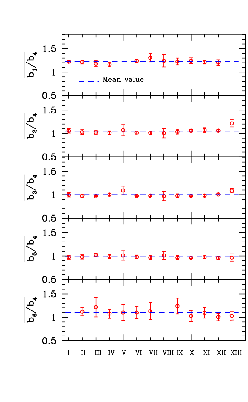
Figure 12.— The relative bias parameters for red galaxies obtained from the correlation functions over $0.98\>h^{-1}{\rm{Mpc}}$ to $9.8\>h^{-1}{\rm{Mpc}}$ using 13 different approaches (see the main text for details). The error-bars are based on the scatter of the data points in the range $0.98\>h^{-1}{\rm{Mpc}}<r_{p}\leq 9.8\>h^{-1}{\rm{Mpc}}$. Panels from top to bottom correspond to the bias parameters for ${\rm Fi_{red}}$ ($i=1,2,3,5,6$), normalized by that of ${\rm F4_{red}}$. The horizontal axis labels the different approaches that are used to determine the bias parameter for each subsamples. Some data points are missing, because the redshift overlap between F1 and F6 is too small to measure their cross-correlation function reliably.

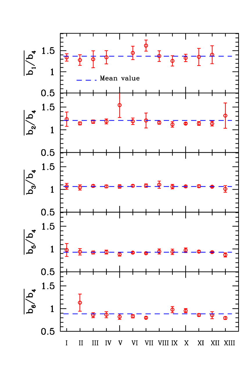
Figure 13.— The same as Fig. 12 for blue galaxies. Panels from top to bottom correspond to the bias parameters for ${\rm Fi_{blue}}$ ($i=1,2,3,5,6$), normalized by that of ${\rm F4_{blue}}$.

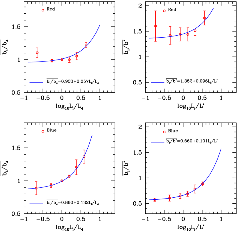
Figure 14.— Left panels: The average relative bias parameter, obtained using the correlation data in $0.98\>h^{-1}{\rm{Mpc}}<r_{p}\leq 9.8\>h^{-1}{\rm{Mpc}}$ as a function of galaxy luminosity, for red (upper panel) and blue (lower panel) galaxies. The results are obtained using the flux-limited samples, and both the bias parameters and the luminosities are normalized by the values of ${\rm F4_{red}}$ and ${\rm F4_{blue}}$, respectively. For a given luminosity, the mean and error-bar are based on the different measurements shown in Figs. 12 and 13. The solid curves show fits to the data. Right panels: The same as the left panels, except that here the bias parameters and the luminosities are normalized by the values for $L^{*}$ galaxies.

In order to study how galaxy clustering depends on both galaxy luminosity and color, we have subdivided each flux-limited sample, Fi, into a red and a blue subsample according to the criteria described in equation (2). We remind that these subsamples are referred to as ${\rm Fi_{red}}$ and ${\rm Fi_{blue}}$. We have carried out the same analyses as described in Section 4 for these color samples. Figs. 8 shows the correlation lengths $r_{0}$ and slopes $\alpha$ obtained by fitting the correlation functions in the range $0.98\>h^{-1}{\rm{Mpc}}\leq r_{p}\leq 9.6\>h^{-1}{\rm{Mpc}}$; the corresponding results for small scales, $0.16\>h^{-1}{\rm{Mpc}}\leq r_{p}\leq 0.98\>h^{-1}{\rm{Mpc}}$, are shown in Figs. 9. In both figures, we also include the results for the total samples (i.e. without color separation) for comparison. Again, the error-bars are obtained from the scatter among the three regions in the SDSS observations. To make the results accessible to others, we list all the values of $r_{0}$ and $\alpha$ in Tables 7 (red galaxies; large scales), 8 (red galaxies; small scales), 9 (blue galaxies; large scales), and 10 (blue galaxies; small scales). In all these tables, we also include the best fit values for $r_{0}$ by fixing $\alpha={\overline{\alpha}}$.

As one can see clearly from the left panels in Fig. 8, on large scales red galaxies in all cases have larger $r_{0}$ than all galaxies and blue galaxies in the same luminosity bin. Note also that the luminosity dependence of $r_{0}$ is seen in all, red and blue samples, although the dependence is stronger for blue galaxies, as to be quantified in the following. Overall, the correlation slope, $\alpha$ (shown in the right panel of Fig. 8), is larger for red galaxies, and the dependence is stronger for the cases where at least one of the two samples in cross-correlation is faint.

As shown in Fig. 9, the correlation lengths $r_{0}$ obtained from the projected 2PCFs on small scales have properties similar to those on large scales, in that red galaxies have a larger correlation length. But the trend is quite different in detail. Firstly, the difference between the correlation lengths obtained from the cross correlations of the brightest red sample ($\rm F1_{red}$) with other red samples are significantly larger here than that shown in Fig. 8. Since the brightest red galaxies are located predominately in clusters and rich groups, this suggests that many of the faint red galaxies are also in clusters and groups. Secondly, for $\rm F3_{red}$ through $\rm F5_{red}$, their cross-correlation with the faintest red galaxies has an amplitude that is significantly larger than their cross-correlation with brighter (except the brightest) red galaxies. This indicates that many red galaxies of intermediate luminosities may possess halos of red satellite galaxies that are more than 1 magnitudes fainter. Finally, on small scales, the luminosity-dependence $r_{0}$ for blue galaxies appears to be weaker.

It is also interesting to look at the cross correlation between red and blue galaxies. In Figs. 10 and 11, we compare the values of $r_{0}$ and $\alpha$ for such cross correlations on large and small scales with those for all galaxies. These values are also listed in Tables 11 and 12. As one can see, on large scales ($0.98\>h^{-1}{\rm{Mpc}}\leq r_{p}\leq 9.6\>h^{-1}{\rm{Mpc}}$) (Fig. 10), the values of $r_{0}$ and $\alpha$ for the red/blue cross-correlation functions are quite similar to those for all galaxies. However, there is a marked difference on small scales ($0.16\>h^{-1}{\rm{Mpc}}\leq r_{p}\leq 0.98\>h^{-1}{\rm{Mpc}}$) (Fig. 11). Here the cross correlation amplitudes between the brightest red galaxies ($\rm F1_{red}$) and blue galaxies are significantly lower than those for all galaxies. Since many of the brightest red galaxies are the brightest central galaxies in clusters and groups, this result suggests the satellite galaxies of these galaxies are preferentially red, in qualitative agreement with the findings by Weinmann et al. (2006).

In order to quantify how galaxies of different colors and luminosities are biased with respect to each other on large scales, we measure the relative bias factors for red and blue galaxies based on the ratios of the corresponding projected 2PCFs, as we did in Section 4 for the luminosity samples. Note that, in addition to the red-red and blue-blue cross-correlation functions among the 6 luminosity bins, one can also use the red-blue cross-correlation functions to obtain the relative bias. These are

$$\frac{b_{i}}{b_{4}}=\frac{W_{Ri,Bj}}{W_{R4,Bj}}\,$$ (9)

for red galaxies, and

$$\frac{b_{i}}{b_{4}}=\frac{W_{Bi,Rj}}{W_{B4,Rj}}\,$$ (10)

for blue galaxies, where $i=1,2,3,5,6$ and $j=1,2,3,4,5,6$, and Bi and Ri denotes ${\rm Fi_{blue}}$ and ${\rm Fi_{red}}$, respectively. In what follows, these six approaches will be referred as approaches VIII, IX, $\cdot\cdot\cdot$, XIII, corresponding to $j=1,2,\cdot\cdot\cdot,6$, respectively. Together with the previous seven approaches, we have now in total 13 approaches to measure the relative bias $b_{i}/b_{4}$ for each red or blue subsamples. Figs. 12 and 13 show the large-scale relative bias factors obtained with the 13 approaches for red and blue galaxies, respectively. Some points are missing again because the overlaps of the samples in question are too small. The dashed line in each panel is the average value of the relative bias. As one can see, most of the approaches give extremely consistent results. The biggest outlier is the one that corresponds to the cross correlation $\rm F2_{red}$-$\rm F6_{blue}$ (approach XIII in the second row of Fig 12), which deviates from the mean bias ratio by just over $2\sigma$.

In the left panels of Fig. 14 (upper panel for red galaxies and lower panel for blue galaxies), we show the average relative bias ($\overline{b_{i}/b_{4}}$ obtained from the 13 approaches) versus luminosity $L_{i}/L_{4}$, where $L_{i}$ for each sample is estimated in the same way as described in Section 4. Fitting to the data with a linear model gives $\overline{b_{i}/b_{4}}=0.953+0.057L_{i}/L_{4}$ for red galaxies, and $\overline{b_{i}/b_{4}}=0.860+0.132L_{i}/L_{4}$ for blue galaxies. As one can see, the luminosity-dependence is much stronger for blue galaxies than for red galaxies. For red galaxies, significant luminosity-dependence is seen only at the brightest end, and there is indication that the bias factor becomes larger for the faintest sample.

In order to put the bias factors for different galaxies in the same absolute scale, we normalize all bias factors relative to that for all the galaxies (blue and red) in the F* sample, i.e. we define

$$\overline{b_{i}/b^{*}}=\overline{b_{i}/b_{4}}\sqrt{\frac{W_{R4,R4}}{W^{*,*}}}$$ (11)

for red galaxies, and

$$\overline{b_{i}/b^{*}}=\overline{b_{i}/b_{4}}\sqrt{\frac{W_{B4,B4}}{W^{*,*}}}$$ (12)

for blue galaxies. Here $W_{R4,R4}$, $W_{B4,B4}$ and $W^{*,*}$ are the projected auto 2PCFs for $F4_{red}$, $F4_{blue}$ and F*, respectively. The values of $\overline{b_{i}/b^{*}}$ versus $L/L^{*}$ are shown in the right panels of Fig. 14 (upper panel for red galaxies and lower panel for blue galaxies). Normalized in this way, the bias factors for red galaxies are all larger than 1, while those for blue galaxies smaller than 1, for the luminosity range probed here. Fitting the luminosity dependence with a linear model, we get $\overline{b_{i}/b^{*}}=1.352+0.096L_{i}/L^{*}$ for red galaxies, and $\overline{b_{i}/b^{*}}=0.560+0.101L_{i}/L^{*}$ for blue galaxies. Note that the constant component in the relation is much larger for red galaxies than for blue galaxies, although the linear terms are now similar. These results are in good agreement with those obtained in Zehavi et al. (2005) based on auto-correlation functions.

6. Non-linear and stochastic bias

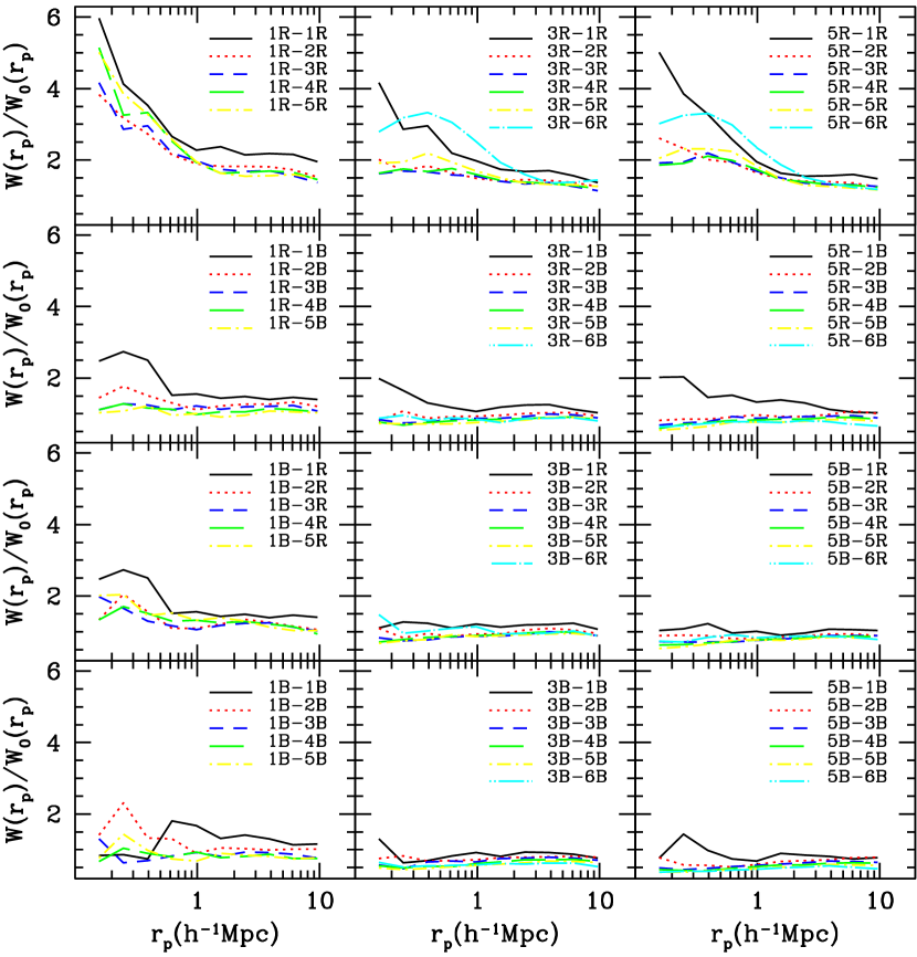
Figure 15.— The ratios between the projected correlation function $W(r_{p})$ and $W_{0}(r_{p})$ for cases with various combinations of color and luminosity, where $W_{0}(r_{p})$ is the power-law fit to the projected correlation function of sample $F^{*}$ on large scales ($r_{0}=5.49\>h^{-1}{\rm{Mpc}}$, $\alpha=1.76$). Three top panels show the results for red galaxies, six middle panels show the results between red and blue galaxies, and three bottom panels show the results for blue galaxies. In each panel, iR-jR denotes ${\rm Fi_{red}}$ with ${\rm Fj_{red}}$, iB-jB denotes ${\rm Fi_{blue}}$ with ${\rm Fj_{blue}}$, iR-jB denotes ${\rm Fi_{red}}$ with ${\rm Fj_{blue}}$.

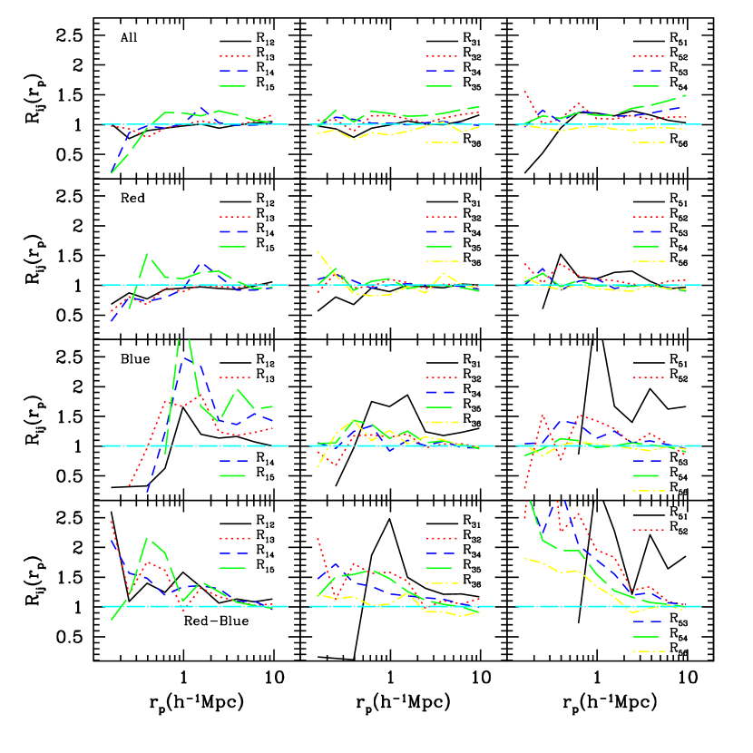
Figure 16.— The value of ${\cal R}_{ij}$ as a function of $r_{p}$ for cases with various combinations of color and luminosity. Panels from top to bottom show results for all-all, red-red, blue-blue, and red-blue samples, respectively. The straight line in each panel shows ${\cal R}_{ij}=1$.

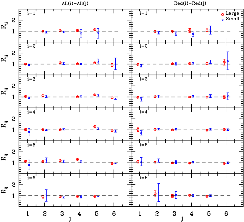
Figure 17.— The ratio ${\cal R}_{ij}$ defined in equation (18) for all (left panels) and red (right panels) galaxies. In all panels, circles show results based on data on large scales, $0.98\>h^{-1}{\rm{Mpc}}\leq r_{p}\leq 9.6\>h^{-1}{\rm{Mpc}}$, while crosses show results based data on small scales, $0.16\>h^{-1}{\rm{Mpc}}\leq r_{p}\leq 0.98\>h^{-1}{\rm{Mpc}}$. From top to bottom are results for $i=1,2,3,4,5,6$, respectively. The value of $j$ for each case is labeled on the horizontal axis. The dashed line in each panel shows ${\cal R}_{ij}=1$. The error-bars are estimated using the scatter of the data points on large scales $0.98\>h^{-1}{\rm{Mpc}}\leq r_{p}\leq 9.6\>h^{-1}{\rm{Mpc}}$ and small scales $0.16\>h^{-1}{\rm{Mpc}}\leq r_{p}\leq 0.98\>h^{-1}{\rm{Mpc}}$, respectively.

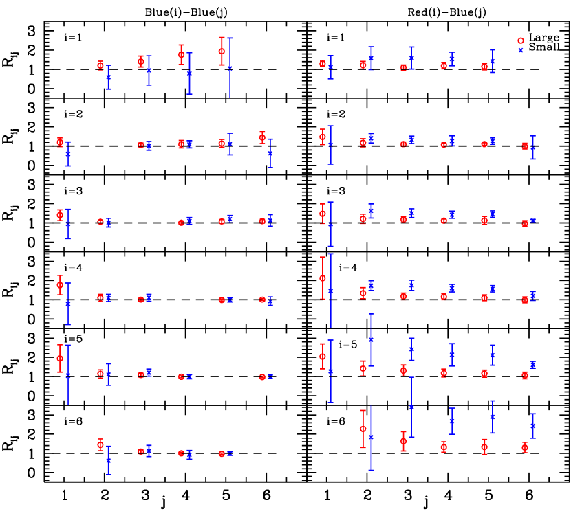
Figure 18.— The same as Fig.  17, but here results are shown for blue versus blue galaxies (left panels) and red versus blue galaxies (right panels).

Table 13The average value of ${\cal R}_{ij}$ over the large scales ($0.98\>h^{-1}{\rm{Mpc}}\leq r_{p}\leq 9.6\>h^{-1}{\rm{Mpc}}$)

Sample	${\rm F1}$	${\rm F2}$	${\rm F3}$	${\rm F4}$	${\rm F5}$	${\rm F6}$
${\rm F1}$		$1.00\pm 0.04$	$1.05\pm 0.06$	$1.05\pm 0.11$	$1.14\pm 0.08$
${\rm F2}$	$1.00\pm 0.04$		$1.13\pm 0.06$	$1.02\pm 0.03$	$1.12\pm 0.02$	$0.91\pm 0.14$
${\rm F3}$	$1.05\pm 0.06$	$1.13\pm 0.06$		$1.02\pm 0.02$	$1.20\pm 0.06$	$0.93\pm 0.08$
${\rm F4}$	$1.05\pm 0.11$	$1.02\pm 0.03$	$1.02\pm 0.02$		$1.30\pm 0.13$	$0.93\pm 0.05$
${\rm F5}$	$1.14\pm 0.08$	$1.12\pm 0.02$	$1.20\pm 0.06$	$1.30\pm 0.13$		$0.94\pm 0.02$
${\rm F6}$		$0.91\pm 0.14$	$0.93\pm 0.08$	$0.93\pm 0.05$	$0.94\pm 0.02$
	${\rm F1_{red}}$	${\rm F2_{red}}$	${\rm F3_{red}}$	${\rm F4_{red}}$	${\rm F5_{red}}$	${\rm F6_{red}}$
${\rm F1_{red}}$		$0.98\pm 0.05$	$0.98\pm 0.05$	$1.05\pm 0.19$	$1.09\pm 0.12$
${\rm F2_{red}}$	$0.98\pm 0.05$		$1.02\pm 0.05$	$1.04\pm 0.06$	$1.06\pm 0.05$	$1.17\pm 0.27$
${\rm F3_{red}}$	$0.98\pm 0.05$	$1.02\pm 0.05$		$0.99\pm 0.03$	$0.99\pm 0.07$	$0.98\pm 0.13$
${\rm F4_{red}}$	$1.05\pm 0.19$	$1.04\pm 0.06$	$0.99\pm 0.03$		$0.97\pm 0.04$	$1.03\pm 0.08$
${\rm F5_{red}}$	$1.09\pm 0.12$	$1.06\pm 0.05$	$0.99\pm 0.07$	$0.97\pm 0.04$		$0.94\pm 0.03$
${\rm F6_{red}}$		$1.17\pm 0.27$	$0.98\pm 0.13$	$1.03\pm 0.08$	$0.94\pm 0.03$
	${\rm F1_{blue}}$	${\rm F2_{blue}}$	${\rm F3_{blue}}$	${\rm F4_{blue}}$	${\rm F5_{blue}}$	${\rm F6_{blue}}$
${\rm F1_{blue}}$		$1.20\pm 0.23$	$1.41\pm 0.28$	$1.76\pm 0.51$	$1.94\pm 0.71$
${\rm F2_{blue}}$	$1.20\pm 0.23$		$1.06\pm 0.09$	$1.10\pm 0.19$	$1.14\pm 0.21$	$1.45\pm 0.31$
${\rm F3_{blue}}$	$1.41\pm 0.28$	$1.06\pm 0.09$		$1.01\pm 0.07$	$1.08\pm 0.10$	$1.10\pm 0.10$
${\rm F4_{blue}}$	$1.76\pm 0.51$	$1.10\pm 0.19$	$1.01\pm 0.07$		$0.99\pm 0.05$	$1.01\pm 0.05$
${\rm F5_{blue}}$	$1.94\pm 0.71$	$1.14\pm 0.21$	$1.08\pm 0.10$	$0.99\pm 0.05$		$0.98\pm 0.04$
${\rm F6_{blue}}$		$1.45\pm 0.31$	$1.10\pm 0.10$	$1.01\pm 0.05$	$0.98\pm 0.04$
	${\rm F1_{blue}}$	${\rm F2_{blue}}$	${\rm F3_{blue}}$	${\rm F4_{blue}}$	${\rm F5_{blue}}$	${\rm F6_{blue}}$
${\rm F1_{red}}$	$1.31\pm 0.12$	$1.22\pm 0.20$	$1.10\pm 0.13$	$1.19\pm 0.16$	$1.14\pm 0.17$
${\rm F2_{red}}$	$1.49\pm 0.40$	$1.18\pm 0.21$	$1.10\pm 0.11$	$1.08\pm 0.08$	$1.11\pm 0.06$	$1.00\pm 0.15$
${\rm F3_{red}}$	$1.48\pm 0.50$	$1.21\pm 0.24$	$1.18\pm 0.15$	$1.12\pm 0.08$	$1.13\pm 0.21$	$0.98\pm 0.14$
${\rm F4_{red}}$	$2.12\pm 1.10$	$1.35\pm 0.28$	$1.18\pm 0.17$	$1.16\pm 0.15$	$1.10\pm 0.15$	$1.00\pm 0.16$
${\rm F5_{red}}$	$2.05\pm 0.65$	$1.42\pm 0.39$	$1.31\pm 0.29$	$1.18\pm 0.20$	$1.15\pm 0.19$	$1.06\pm 0.17$
${\rm F6_{red}}$		$2.27\pm 0.96$	$1.63\pm 0.50$	$1.33\pm 0.27$	$1.33\pm 0.40$	$1.31\pm 0.28$

Table 14The average value of ${\cal R}_{ij}$ over the small scales ($0.16\>h^{-1}{\rm{Mpc}}\leq r_{p}\leq 0.98\>h^{-1}{\rm{Mpc}}$)

Sample	${\rm F1}$	${\rm F2}$	${\rm F3}$	${\rm F4}$	${\rm F5}$	${\rm F6}$
${\rm F1}$		$0.92\pm 0.10$	$0.92\pm 0.08$	$0.80\pm 0.34$	$0.81\pm 0.44$
${\rm F2}$	$0.92\pm 0.10$		$1.07\pm 0.11$	$1.00\pm 0.07$	$1.23\pm 0.23$	$1.03\pm 0.53$
${\rm F3}$	$0.92\pm 0.08$	$1.07\pm 0.11$		$1.05\pm 0.06$	$1.13\pm 0.12$	$0.84\pm 0.06$
${\rm F4}$	$0.80\pm 0.34$	$1.00\pm 0.07$	$1.05\pm 0.06$		$1.12\pm 0.07$	$0.90\pm 0.11$
${\rm F5}$	$0.81\pm 0.44$	$1.23\pm 0.23$	$1.13\pm 0.12$	$1.12\pm 0.07$		$0.95\pm 0.04$
${\rm F6}$		$1.03\pm 0.53$	$0.84\pm 0.06$	$0.90\pm 0.11$	$0.95\pm 0.04$
	${\rm F1_{red}}$	${\rm F2_{red}}$	${\rm F3_{red}}$	${\rm F4_{red}}$	${\rm F5_{red}}$	${\rm F6_{red}}$
${\rm F1_{red}}$		$0.84\pm 0.11$	$0.78\pm 0.16$	$0.73\pm 0.20$	$1.09\pm 0.38$
${\rm F2_{red}}$	$0.84\pm 0.11$		$1.03\pm 0.13$	$1.06\pm 0.08$	$1.20\pm 0.15$	$1.29\pm 0.81$
${\rm F3_{red}}$	$0.78\pm 0.16$	$1.03\pm 0.13$		$1.06\pm 0.09$	$1.08\pm 0.14$	$1.06\pm 0.32$
${\rm F4_{red}}$	$0.73\pm 0.20$	$1.06\pm 0.08$	$1.06\pm 0.09$		$1.06\pm 0.09$	$1.02\pm 0.08$
${\rm F5_{red}}$	$1.09\pm 0.38$	$1.20\pm 0.15$	$1.08\pm 0.14$	$1.06\pm 0.09$		$1.01\pm 0.08$
${\rm F6_{red}}$		$1.29\pm 0.81$	$1.06\pm 0.32$	$1.02\pm 0.08$	$1.01\pm 0.08$
	${\rm F1_{blue}}$	${\rm F2_{blue}}$	${\rm F3_{blue}}$	${\rm F4_{blue}}$	${\rm F5_{blue}}$	${\rm F6_{blue}}$
${\rm F1_{blue}}$		$0.60\pm 0.62$	$0.95\pm 0.76$	$0.79\pm 1.08$	$1.05\pm 1.58$
${\rm F2_{blue}}$	$0.60\pm 0.62$		$1.02\pm 0.22$	$1.10\pm 0.19$	$1.11\pm 0.56$	$0.63\pm 0.73$
${\rm F3_{blue}}$	$0.95\pm 0.76$	$1.02\pm 0.22$		$1.11\pm 0.18$	$1.21\pm 0.18$	$1.13\pm 0.30$
${\rm F4_{blue}}$	$0.79\pm 1.08$	$1.10\pm 0.19$	$1.11\pm 0.18$		$1.00\pm 0.11$	$0.93\pm 0.22$
${\rm F5_{blue}}$	$1.05\pm 1.58$	$1.11\pm 0.56$	$1.21\pm 0.18$	$1.00\pm 0.11$		$1.00\pm 0.09$
${\rm F6_{blue}}$		$0.63\pm 0.73$	$1.13\pm 0.30$	$0.93\pm 0.22$	$1.00\pm 0.09$
	${\rm F1_{blue}}$	${\rm F2_{blue}}$	${\rm F3_{blue}}$	${\rm F4_{blue}}$	${\rm F5_{blue}}$	${\rm F6_{blue}}$
${\rm F1_{red}}$	$1.12\pm 0.61$	$1.58\pm 0.60$	$1.59\pm 0.57$	$1.54\pm 0.35$	$1.43\pm 0.59$
${\rm F2_{red}}$	$1.07\pm 0.99$	$1.41\pm 0.25$	$1.33\pm 0.19$	$1.28\pm 0.26$	$1.26\pm 0.17$	$0.94\pm 0.60$
${\rm F3_{red}}$	$0.94\pm 1.15$	$1.63\pm 0.37$	$1.51\pm 0.23$	$1.43\pm 0.19$	$1.47\pm 0.17$	$1.12\pm 0.08$
${\rm F4_{red}}$	$1.46\pm 1.94$	$1.74\pm 0.25$	$1.75\pm 0.27$	$1.60\pm 0.20$	$1.57\pm 0.16$	$1.20\pm 0.24$
${\rm F5_{red}}$	$1.28\pm 1.62$	$2.91\pm 1.35$	$2.42\pm 0.57$	$2.13\pm 0.58$	$2.11\pm 0.52$	$1.62\pm 0.18$
${\rm F6_{red}}$		$1.85\pm 1.72$	$3.40\pm 1.55$	$2.68\pm 0.68$	$2.90\pm 0.83$	$2.43\pm 0.63$

In the last two sections we have analyzed the auto- and cross-correlation functions for galaxies of different luminosities and colors. We have seen that on scales $r_{p}\gtrsim 1\>h^{-1}{\rm{Mpc}}$ all correlation functions are roughly parallel, but on smaller scales different galaxies may have different behaviors (see Fig. 5). In order to investigate the scale-dependence of the correlation functions in more detail, we plot in Fig. 15 the ratios between the various projected correlation functions, $W(r_{p})$, and a normalization function, $W_{0}(r_{p})$, which is the power-law fit to the projected correlation function of the sample $F^{*}$ on large scales and corresponds to $r_{0}=5.49\>h^{-1}{\rm{Mpc}}$ and $\alpha=1.76$. Three top panels show results for red galaxies; six middle panels show results between red and blue galaxies; and three bottom panels show results for blue galaxies. Based on the figure, we can draw the following conclusions:

• On scales larger than $1\>h^{-1}{\rm{Mpc}}$, all the correlation functions are roughly parallel, a fact we have mentioned earlier.

• The cross-correlation functions between the brightest red galaxies and other red galaxies have enhanced clustering on scales smaller than $\sim 1\>h^{-1}{\rm{Mpc}}$, and the enhancement is the strongest for the cross-correlation between the brightest and faintest samples.

• The cross-correlation functions among faint blue galaxies, and between faint-blue and faint-red galaxies, appear to be suppressed slightly on scales $\lesssim 1\>h^{-1}{\rm{Mpc}}$ relative to the extrapolations from larger scales.

• The brightest blue galaxies show enhanced correlation with red galaxies of different luminosities on scales $\lesssim 1\>h^{-1}{\rm{Mpc}}$.

Some of these results are expected, as it is well known that red galaxies reside preferentially in rich systems, such as clusters and groups, while faint blue galaxies are distributed in the ‘field’ (i.e., in dark matter haloes of significantly lower mass). Note, however, that the cross-correlation functions between the brightest red galaxies and faint red galaxies are lower than the auto-correlation function of the brightest galaxies on scales $r_{p}\gtrsim 1\>h^{-1}{\rm{Mpc}}$, suggesting that not all faint red galaxies are associated with the brightest red galaxies. There is no enhancement in the cross-correlation functions on small scales between red galaxies and all except the brightest blue galaxies. This again can be explained by the fact that blue galaxies with low and intermediate luminosities are distributed in the field.

One surprising result is that the brightest blue galaxies are strongly correlated with red galaxies on small scales, and in many ways the clustering properties of these galaxies are similar to that of red galaxies with intermediate luminosities. In order to understand this result in more detail, we have examined the properties of this population of galaxies more closely. Using the group catalogue constructed by Yang et al. (2007, in preparation), we find that $\sim 15\%$ ($\sim 80\%$) of the brightest blue galaxies are the central galaxies of groups with masses $\gtrsim 10^{13.5}h^{-1}{\rm M}_{\odot}$ ($\gtrsim 10^{13}h^{-1}{\rm M}_{\odot}$), compared to $\sim 30\%$ ($\sim 85\%$) for the red galaxies in the same luminosity bin. It is therefore possible that a fraction of the brightest blue galaxies are in fact ‘early-type’ galaxies and their relatively blue colors are probably due to rejuvenation of star formation or AGN activities in their centers. Clearly, further analysis is required in order to understand the properties of this population of galaxies in more detail.

Next we discuss how our results may put constraints on the stochasticity/non-linearity in the bias relation. Consider the density field (smoothed on some scale) traced by a population $i$ of galaxies, $\delta_{i}$. In general we may write it in terms of the density field of another population, $\delta_{j}$, as

$$\delta_{i}=B_{ij}\delta_{j}+f_{i}(\delta_{j})+\epsilon_{ij}\,,$$ (13)

where the first term on the right-hand side describes the linear part of the correlation between the two populations, the second term is the non-linear part, and $\epsilon_{ij}$ is the stochastic, uncorrelated part: $\langle\epsilon_{ij}\delta_{j}\rangle=0$. It then follows that

$$\langle\delta_{i}\delta_{j}\rangle=B_{ij}\langle\delta_{j}^{2}\rangle+\langle\delta_{j}f_{i}(\delta_{j})\rangle\,,$$ (14)

and

$$\langle\delta_{i}^{2}\rangle=B_{ij}^{2}\langle\delta_{j}^{2}\rangle+\langle\epsilon_{ij}^{2}\rangle+\langle f_{i}^{2}(\delta_{j})\rangle+2B_{ij}\langle\delta_{j}f_{i}(\delta_{j})\rangle\,.$$ (15)

Thus, for any two populations we can define two relative bias factors, one based on the cross correlation with another population, and one based on the auto-correlation functions of the two populations:

$$B^{\rm(c)}_{ij}\equiv{\langle\delta_{i}\delta_{j}\rangle\over\langle\delta_{j}^{2}\rangle}\,;$$ (16)

$$B^{\rm(a)}_{ij}\equiv\left({\langle\delta_{i}^{2}\rangle\over\langle\delta_{j}^{2}\rangle}\right)^{1/2}\,.$$ (17)

The square of the ratio between these two bias factors is

$${\cal R}_{ij} \equiv \left({B_{ij}^{\rm(a)}\over B_{ij}^{\rm(c)}}\right)^{2}={\langle\delta_{i}^{2}\rangle\langle\delta_{j}^{2}\rangle\over\langle\delta_{i}\delta_{j}\rangle^{2}}$$ (18)

$$= 1+{\langle\epsilon_{ij}^{2}\rangle+\zeta_{ij}\over\langle\delta_{i}\delta_{j}\rangle^{2}/\langle\delta_{j}^{2}\rangle}\,,$$

where

$$\zeta_{ij}\equiv\langle f_{i}^{2}(\delta_{j})\rangle-\langle\delta_{j}f_{i}(\delta_{j})\rangle^{2}/\langle\delta_{j}^{2}\rangle$$ (19)

describes the contribution due to the non-linear part of the relative bias relation. Note that ${\cal R}$ is related to the linear correlation coefficient, $r$, defined in Dekel & Lahav (1999; their eq.[13]) as ${\cal R}=r^{-2}$. For two populations, $i$ and $j$ that are entirely uncorrelated one has that $R_{ij}\rightarrow\infty$, while $R_{ij}=1$ when $i$ and $j$ are perfectly correlated. Both the stochastic component, $\langle\epsilon_{ij}^{2}\rangle$, and the non-linear component, $\zeta_{ij}$, can cause ${\cal R}_{ij}$ to deviate from unity, and in general it is difficult to separate stochasticity from non-linearity. On large scales, however, the non-linear component in the bias relation may be neglected, and we have that

$${\cal R}_{ij}=1+{\langle\epsilon_{ij}^{2}\rangle\over B_{ij}^{2}\langle\delta_{j}^{2}\rangle}\,.$$ (20)

To examine the importance of stochasticity/non-linearity in the relative bias relations, we calculate ${\cal R}_{ij}$ for galaxies of different luminosities and colors. Based on equation (18), we estimate ${\cal R}_{ij}$ using

$${\cal R}_{ij}={W_{ii}W_{jj}\over W_{ij}^{2}}\,,$$ (21)

where $W_{ii}$ and $W_{jj}$ are the auto-correlation functions of subsamples ‘$i$’ and ‘$j$’, respectively, and $W_{ij}$ is the cross- correlation function between the two subsamples. Note that ‘$i$’ and ‘$j$’ denote not only luminosity samples but also color samples. Unlike what we did above, here we estimate $W_{ii}$, $W_{jj}$ and $W_{ij}$ all in the overlapping region of the two samples in question, so that volume effects are minimized.

In Fig 16 we show ${\cal R}_{ij}$ as a function of $r_{p}$ for various combinations of color- and luminosity-samples. The results are quite noisy in some cases, again because of the small overlap of the samples involved. As one can see, for cases where ${\cal R}_{ij}$ is well determined, it is close to 1 for all-all and red-red pairs of samples. For blue-blue pairs, ${\cal R}_{ij}$ is also close to 1 except the cases involving the brightest galaxies where at large scales ${\cal R}_{ij}$ can be significantly larger than 1. As we have discussed above, the brightest blue galaxies have clustering properties different from that of fainter blue galaxies, because a significant fraction of them are, like bright red galaxies, central galaxies of relatively massive groups. For red versus blue galaxies, ${\cal R}_{ij}$ is significantly larger than 1 on small scales. The signal is also more prominent between faint red and faint blue galaxies and can extend to a few $\>h^{-1}{\rm{Mpc}}$.

To show this more clearly, we plot the average value of ${\cal R}_{ij}$ over two different scales. The results are shown in Figs. 17 – 18 and listed in Tables  13 – 14 for all versus all, red versus red, blue versus blue, and red versus blue, respectively. In all the figures, circles show results based on clustering on large scales ($0.98\>h^{-1}{\rm{Mpc}}\leq r_{p}\leq 9.6\>h^{-1}{\rm{Mpc}}$), while crosses show results based on clustering on small scales ($0.16\>h^{-1}{\rm{Mpc}}\leq r_{p}\leq 0.98\>h^{-1}{\rm{Mpc}}$). As one can see, on large scales ($\gtrsim 1\>h^{-1}{\rm{Mpc}}$) ${\cal R}_{ij}$ is very close to 1 for red-red, blue-blue (with the exception of cases involving the brightest blue galaxies), and all-all pairs, but has a value between $1.4$ to $2.2$ for pairs between faint red and blue galaxies. On scales $\lesssim 1\>h^{-1}{\rm{Mpc}}$, the ratio is again very close to 1 for all-all, red-red and blue-blue pairs, but is significantly larger than 1 for red versus blue galaxies and is as large as $\sim 3$ for faint-red versus faint-blue galaxies.

These results suggest that red (or blue) galaxies of different luminosities trace each other almost linearly and in an almost deterministic way on both small and large scales, but there is a significant stochastic/non-linear component in the relationship between red and blue galaxies of different luminosities, and in particular on small scales. The large value of $R_{ij}$ on small scales between red and blue galaxies (except the brightest blue galaxies) is almost certainly due to the fact that blue galaxies of low and intermediate luminosities avoid dense groups and clusters while red galaxies reside preferentially in such places. The fact that such stochastic/non-linear component extends to a few $\>h^{-1}{\rm{Mpc}}$ (see Fig. 16) suggests that the clustering of clusters and groups on large scales may produce segregation of the galaxy population on large scales.

7. Summary

In this paper, we use galaxy samples constructed from the SDSS Data Release 4 (DR4) to study the cross-correlation functions between galaxies with different luminosities and colors. Galaxies are separated at $g-r=-0.7-0.032(M_{r,0.1}+16.5)$ into red and blue samples according to their colors, and each of the color samples is further divided into 6 subsamples according to luminosity. We measure the projected two-point correlation function for each subsample, and the projected cross-correlation for each pair of subsamples. Each correlation function is fitted with power laws over two different ranges of separations: $0.98\>h^{-1}{\rm{Mpc}}\leq r_{p}\leq 9.6\>h^{-1}{\rm{Mpc}}$ and $0.16\>h^{-1}{\rm{Mpc}}\leq r_{p}\leq 0.98\>h^{-1}{\rm{Mpc}}$, and each of the power laws are characterized by a correlation length, $r_{0}$, and a logarithmic slope, $\alpha$. Our main results can be summarized as follows:

1. At projected separations $r_{p}\gtrsim 1\>h^{-1}{\rm{Mpc}}$, all correlation functions are roughly parallel to each other (but see exceptions for the brightest galaxies with $-22.0\geq M_{r,0.1}\geq-23.0$ in Zehavi et al. 2005; Li et al. 2006), but on smaller scales different populations of galaxies have different behaviors.

2. The auto- and cross-correlation functions of red galaxies on $r_{p}\lesssim 1\>h^{-1}{\rm{Mpc}}$ are significantly enhanced relative to those on larger scales. The effect is the strongest between the brightest red galaxies and other red galaxies. Such enhancement is absent for blue galaxies and in the cross-correlation between red and blue galaxies.

3. For blue galaxies the luminosity-dependence of the correlation amplitude on large scales is strong over the entire luminosity range, while for red galaxies the dependence is weaker and becomes insignificant for luminosities below $L^{*}$. There is an indication that the luminosity-dependence may inverse at the faint end.

4. For a given luminosity, red galaxies are more strongly clustered than blue galaxies on both large and small scales, and the difference is larger for fainter luminosities.

5. One large scale, the bias factors of a given population of galaxies obtained from its cross correlations with other populations of galaxies are similar, and comparable to that based on the auto-correlation function.

6. On both large and small scales, the ratio ${\cal R}_{ij}$ is very close to 1 for red (or blue except the brightest) galaxies of different luminosities, suggesting that the bias relations between red (or blue) galaxies of different luminosities are close to linear and deterministic.

7. On scales $\lesssim 1\>h^{-1}{\rm{Mpc}}$, $R_{ij}$ is significantly larger than 1 between red and blue galaxies and as large as $\sim 2$ between faint red and faint blue galaxies, suggesting that a significant stochastic/non-linear component exists in the bias relations between blue and red galaxies on small scales.

8. The clustering properties of the brightest blue galaxies resemble more that of red galaxies of intermediate luminosities than that of fainter blue galaxies, indicating that a significant fraction of them are located in relative rich systems.

The results obtained in this paper provide important information about the relationships between the spatial distributions of galaxies of different properties in space. Part of our findings are consistent with previous probes (e.g. the luminosity and color dependences of SDSS galaxies based on the auto correlation functions by Zehavi et al. 2005; Li et al. 2006). Most of our findings will put new constraints on the galaxy formation models. To explore the implications of our findings for galaxy formation in the cosmic density field, the results obtained here should be combined with semi-analytical and/or halo occupation models to constrain how galaxies populate dark matter halos, and how galaxies are distributed in individual dark matter halos. We will come back to this in the future.

During the final stages of this project a paper appeared by Swanson et al. (2007), who carried out a similar investigation to study the relative biases for galaxies of different luminosities and colors. Although their analysis is based on counts-in-cells, as opposed to the correlation functions used here, their results are qualitatively similar to ours. A detailed comparison, however, is complicated because of the differences in the statistical methods and sample selections.

References

- Adelman-McCarthy et al. (2006) Adelman-McCarthy J. K., Agüeros M. A., Allam S. S., Anderson K. S. J., Anderson S. F., Annis J., Bahcall N. A., Baldry I. K., et al., 2006, ApJS, 162, 38
- (2) Baldry I.K., Glazebrook K., Brinkmann J., Ivezić Ž., Lupton R.H., Nichol R.C., Szalay A.S., 2004, ApJ, 600, 681
- (3) Bell E.F., et al., 2004, ApJ, 608, 752
- Benoist et al. (1996) Benoist, C., Maurogordato, S., da Costa, L. N., Cappi, A., & Schaeffer, R. 1996, ApJ, 472, 452
- Berlind & Weinberg (2002) Berlind A. A., Weinberg D. H., 2002, ApJ, 575, 587
- Blanton et al. (2003a) Blanton M. R., Brinkmann J., Csabai I., Doi M., Eisenstein D., Fukugita M., Gunn J. E., Hogg D. W., et al., 2003a, AJ, 125, 2348
- Blanton et al. (2003b) Blanton M. R., Hogg D. W., Bahcall N. A., Brinkmann J., Britton M., Connolly A. J., Csabai I., Fukugita M., et al., 2003b, ApJ, 592, 819
- (8) Blanton M. R., et al., 2003c, ApJ, 594, 186
- Blanton etal (2005) Blanton M. R., et al., 2005, AJ, 129, 2562
- Brown, Webster & Boyle (2000) Brown, M. J. I., Webster, R. L., & Boyle, B. J. 2000, MNRAS, 317, 782
- Boerner et al. (1989) Börner, G., Mo, H., & Zhou, Y. 1989, A&A, 221, 191
- Budavari et al. (2003) Budavari, T., et al., 2003, ApJ, 595, 59
- Cooray & Sheth (2002) Cooray A., Sheth R., 2002, PhR, 372, 1
- Peebles (1983) Davis, M., Peebles, P.J.E. 1983, ApJ 267,465
- (15) Dekel A., Lahav O., 1999, ApJ, 520, 24
- Guzzo et al. (1997) Guzzo, L., Strauss, M. A., Fisher, K. B., Giovanelli, R., & Haynes, M. P. 1997, ApJ, 489, 37
- Goto et al. (2003) Goto, T., Yamauchi, C., Fujita, Y., Okamura, S., Sekiguchi, M., Smail, I., Bernardi, M., & Gomez, P. L. 2003, MNRAS346, 601
- Hamilton & Tegmark (2004) Hamilton, A. J. S. & Tegmark, M. 2004, MNRAS, 349, 115
- (19) Hogg D.W., et al., 2004, ApJ, 601, L29
- Jing et al. (1991) Jing, Y. P., Mo, H. J., & Boerner, G. 1991, A&A, 252, 449
- Jing, Mo, & Börner (1998) Jing, Y. P., Mo, H. J., & Börner, G. 1998, ApJ, 494, 1
- Li et al. (2006) Li, C., Kauffmann, G., Jing, Y.P., White, S. D. M., Boerner, G., Cheng, F.Z. 2006, MNRAS, 368, 21
- Loveday et al. (1995) Loveday, J., Maddox, S. J., Efstathiou, G., & Peterson, B. A. 1995, ApJ, 442, 457
- Madgwick et al. (2003) Madgwick, D. S. et al. 2003, MNRAS, 344, 847
- (25) Mo H.J., White S.D.M., 1996, 282, 347
- Norberg et al. (2001) Norberg, P., et al. 2001, MNRAS, 328, 64
- Norberg et al. (2002) Norberg, P., et al. 2002, MNRAS, 332, 827
- Park et al. (1994) Park, C., Vogeley, M. S., Geller, M. J., & Huchra, J. P. 1994, ApJ, 431, 569
- Peacock & Smith (2000) Peacock J. A., Smith R. E., 2000, MNRAS, 318, 1144
- Peebles (1980) Peebles, P.J.E. 1980, The Large-Scale Structure of the Universe, Princeton University Press, Princeton
- Seljak (2000) Seljak U., 2000, MNRAS, 318, 203
- (32) Swanson M.E.C., Tegmark M., Blanton M., Zehavi I., 2007, preprint (astro-ph/0702584)
- van den Bosch, Mo, & Yang (2003) van den Bosch, F. C., Yang, X., Mo, H. J., 2003, MNRAS, 340, 771
- Weinmann (2006) Weinmann, S.M., van den Bosch, F. C., Yang, X.H., Mo, H. J., Croton, D. J., Moore, B., 2006, MNRAS, 366, 2
- Willmer, da Costa & Pellegrini (1998) Willmer, C. N. A., da Costa, L. N., & Pellegrini, P. S. 1998, AJ, 115, 869
- Yang, Mo, & van den Bosch (2003) Yang, X., Mo, H. J., van den Bosch, F. C., 2003, MNRAS, 339, 1057
- Yang, Mo, & van den Bosch (2005) Yang, X., Mo, H. J., van den Bosch, F. C., Weinmann, S.M., C., Li, Y.P., Jing, 2005, MNRAS, 362, 711
- York etal (2000) York, D. G., et al., 2000, AJ, 120, 1579
- Zehavi etal (2002) Zehavi, I., et al., 2002, ApJ, 571, 172
- Zehavi et al. (2005) Zehavi I., et al., 2005, ApJ, 630, 1