On model selection forecasting, Dark Energy and modified gravity

Abstract

The Fisher matrix approach (Fisher (1935)) allows one to calculate in advance how well a given experiment will be able to estimate model parameters, and has been an invaluable tool in experimental design. In the same spirit, we present here a method to predict how well a given experiment can distinguish between different models, regardless of their parameters. From a Bayesian viewpoint, this involves computation of the Bayesian evidence. In this paper, we generalise the Fisher matrix approach from the context of parameter fitting to that of model testing, and show how the expected evidence can be computed under the same simplifying assumption of a gaussian likelihood as the Fisher matrix approach for parameter estimation. With this ‘Laplace approximation’ all that is needed to compute the expected evidence is the Fisher matrix itself. We illustrate the method with a study of how well upcoming and planned experiments should perform at distinguishing between Dark Energy models and modified gravity theories. In particular we consider the combination of 3D weak lensing, for which planned and proposed wide-field multi-band imaging surveys will provide suitable data, and probes of the expansion history of the Universe, such as proposed supernova and baryonic acoustic oscillations surveys. We find that proposed large-scale weak lensing surveys from space should be able readily to distinguish General Relativity from modified gravity models.

1 Introduction

While the goal of parameter estimation is to determine the best fit values (and the errors) of a set of parameters within a model, model selection seeks to distinguish between different models, which in general will have different sets of parameters. Model selection has received attention in cosmology only relatively recently (starting with Jaffe (1996)). Only in recent years have cosmological data had enough statistical power to address the problem, although elsewhere in astronomy model selection has been applied for some time (e.g. Lucy & Sweeney (1971)).

For parameter estimation, the Fisher matrix approach (Fisher (1935)) has been invaluable in experimental design. It allows one to forecast how well a given experiment will be able to estimate model parameters. In the same spirit, one may want to predict how well a given experiment can distinguish between different models.

Of particular interest is the case of nested models, where the more complicated model has additional parameters, in addition to those in the simpler model. The simpler model may be interpreted as a particular case for the more complex model where the additional parameters are kept fixed at some fiducial values. The additional parameters may be an indication of new physics, thus the question one may ask is: “would the experiment provide data with enough statistical power to require additional parameters and therefore to signal the presence of new physics if the new physics is actually the true underlying model?”

Examples of this type of questions are: “does the primordial power spectrum deviate from scale invariance?”, “do the data require a running of the primordial power spectrum spectral index?”, “do observations require a dark energy that deviates from a cosmological constant with equation of state parameter $w=-1$?” etc. (e.g. Liddle et al. (2006); Bridges, Lasenby & Hobson (2006); Mukherjee et al. (2006); Parkinson, Mukherjee & Liddle (2006); Saini et al. (2004); Bridges, Lasenby & Hobson (2007); Trotta (2007) and references therein).

In this paper we present a general statistical method for rapidly calculating in advance how well a given experimental design can be expected to distinguish between competing (and in particular nested) theoretical models for the data, under the Laplace approximation.

We then present an application of the method to the cosmological context: we forecast how three proposed weak lensing experiments may distinguish between Dark Energy (e.g. Peebles & Ratra (1988); Wetterlich (1988) and modified gravity models (e.g. Dvali, Gabadaze & Porrati (2000) (DGP)).

The standard cosmological model is extremely successful: with only 6 parameters it fits a host of observations and provides a description of the Universe from z=1100 to present day. This finding is in good agreement with what can be expected of current data, based on Bayesian complexity theory ((Kunz, Trotta & Parkinson (2006)). The parameters of the model are tightly constrained, many at the percent level, and there is a considerable weight of evidence in favour of a substantial contribution of Dark Energy. Alternative explanations for the apparent Dark Energy are a Cosmological Constant, a slowly rolling scalar field or a fluid component, whose effects on the expansion history can be described by an equation of state parameter which may evolve in time, or a large-scale modification to General Relativity.

Each of these can be described as a different model. An interesting question is which of these possibilities is favoured by the data. In contrast to parameter estimation, this is an issue of model selection, which has been the subject of recent attention in cosmology (e.g. Hobson, Bridle & Lahav (2002); Saini et al. (2004); Mukherjee, Parkinson & Liddle (2006); Liddle et al. (2006); Szydlowski & Godlowski (2006a, b); Pahud et al. (2006, 2007); Serra, Heavens & Melchiorri (2007) and references therein). In particular, Mukherjee et al. (2006); Trotta (2006) compare evolving dark energy models with a cosmological constant.

Dark Energy has potentially measurable effects through its effect on both the expansion history of the Universe, and through the growth rate of perturbations. Some methods, such as study of the luminosity distance of Type Ia supernovae (SN; e.g. Riess et al. (1998)), baryonic acoustic oscillations (BAO; e.g. Eisenstein & Hu (1998)) or geometric weak lensing methods (e.g. Taylor et al. (2007)), probe only the expansion history, whereas others such as 3D cosmic shear weak lensing or cluster counts can probe both. Combinations of various probes promise very accurate determinations of the equation of state (e.g. Heavens, Kitching & Taylor (2006)).

For methods based on probing the expansion history alone, there is a difficulty in that the same expansion history of a universe where the law of gravity has been modified on large scales can also be obtained in a universe with standard General Relativity but a dark energy component with a suitable equation of state parameter $w(z)$. In general however the growth history of cosmological structures will be different in the two cases (e.g. Huterer & Linder (2006), but see Kunz & Sapone (2006)).

Therefore in principle there are advantages in using methods which also probe the growth rate, such as 3D weak lensing. It becomes a very interesting question to ask whether such methods could distinguish between the Dark Energy and modified gravity scenarios.

This question may be answered in a Bayesian context by considering the Bayesian Factor, which is the ratio of the Bayesian Evidences, i.e. the ratio of probabilities of the data given the two models. The evidence ratio may be generalised to a genuine posterior probability of the models by multiplying by a ratio of priors of the models. The evidence involves an integration of the likelihood, multiplied by priors, over the parameter space of each model, and this can be computationally expensive if the dimension of the parameter space is large. By making a simplifying assumption in the spirit of Fisher’s analysis, one can compute the expected evidence for a given experiment, in advance of taking any data, and forecast the extent to which an experiment may be able to distinguish between different models. The Fisher matrix approach in parameter estimation assumes that the expected behaviour of the likelihood $L$ near the maximum characterises the likelihood sufficiently well to be used to estimate errors on the parameters (i.e. the Taylor expansion of $\ln L$ to include second-order terms holds at least until $\ln L$ drops by $\sim 1$). The Fisher Matrix is defined by

$$F_{\alpha\beta}\equiv-\left\langle\frac{\partial^{2}\ln L}{\partial\theta_{\alpha}\theta_{\beta}}\right\rangle$$ (1)

where $\theta_{\alpha}$ are the model parameters, and $\langle\ln L\rangle\simeq\langle\ln L^{0}\rangle-F_{\alpha\beta}\left[\theta_{\alpha}-\theta_{\alpha}^{0}\right]\left[\theta_{\beta}-\theta_{\beta}^{0}\right]/2$, where $0$ indicates peak values. In this paper, we compute the expected evidence by assuming that we can ignore higher-order terms in the Taylor expansion throughout. This allows a major simplification, called the Laplace approximation, in that the expected evidence can be computed directly from the Fisher Matrix at essentially no extra cost. Of course, one must make the caveat that the quadratic expansion of $\ln L$ may be a poor approximation in some cases, but nevertheless the computation of the expected evidence may be a useful first step.

The layout of this paper is that we present the formal computation of the ratio of expected evidences (also called the Bayes factor) in Section 2, and apply the method to a combination planned and proposed data sets (3D weak lensing, microwave background measurements, supernovae and baryonic acoustic oscillations probes) in Section 3.

2 Forecasting Evidence

The aim here is to compute the Bayesian Evidence ratio for two different models, i.e. given a dataset arising from a true model, we want to know the probability with which a second model can be ruled out.

The spirit of this is very similar to the Fisher Matrix approach for parameter estimation, where one computes the expected likelihood as a function of parameters, in the absence of data.

We make the approximation that the expected likelihood is everywhere accurately described by a multivariate Gaussian, with a curvature given by a Taylor expansion at the expected peak. Thus it should be regarded as a first step; more sophisticated simulation techniques may be necessary if this assumption is not adequate. A special case of this was recently presented by Trotta (2007). However, it is worth pointing out that it is routine to compute expected marginal errors on parameters using the inverse of the Fisher matrix. This is equivalent to assuming the Laplace approximation, and doing only one fewer integration than we propose here. In some cases, the approximation works very well (see e.g. Cornish N.J., Crowder J. (2005)), but there are certainly some examples where the approximation is not particularly accurate (e.g. Wang et al. (2004)). For the Planck microwave background experiment we find reasonable agreement between Fisher and Monte Carlo Markov Chain errors (to within about 30%), if the same likelihood calculations are used for both. Note that for this paper, we follow Hu (2002) for the likelihood, which is accurate for the noise-dominated regime. For Planck, the errors will therefore be rather conservative.

The other approximations we make are that the priors on the parameters are uniform, but this could be relaxed to Gaussians if desired. We also assume that the priors on the two models are the same; this could easily be relaxed as it just adjusts the normalisation.

2.1 Models and Notation

We denote two competing models by $M$ and $M^{\prime}$. We assume that $M^{\prime}$ is a simpler model, which has fewer ($n^{\prime}<n$) parameters in it. We further assume that it is nested in Model $M^{\prime}$, i.e. the $n^{\prime}$ parameters of model $M^{\prime}$ are common to $M$, which has $p\equiv n-n^{\prime}$ extra parameters in it. These parameters are fixed to fiducial values in $M^{\prime}$.

We denote by $D$ the data vector, and by $\theta$ and $\theta^{\prime}$ the parameter vectors (of length $n$ and $n^{\prime}$).

The posterior probability of each model comes from Bayes’ theorem:

$$p(M|D)=\frac{p(D|M)p(M)}{p(D)}$$ (2)

and similarly for $M^{\prime}$. By marginalisation $p(D|M)$, known as the Evidence, is

$$p(D|M)=\int d\theta\,p(D|\theta,M)p(\theta|M),$$ (3)

which should be interpreted as a multidimensional integration. Hence the posterior relative probabilities of the two models, regardless of what their parameters are, is

$$\frac{p(M^{\prime}|D)}{p(M|D)}=\frac{p(M^{\prime})}{p(M)}\frac{\int d\theta^{\prime}\,p(D|\theta^{\prime},M^{\prime})p(\theta^{\prime}|M^{\prime})}{\int d\theta\,p(D|\theta,M)p(\theta|M)}.$$ (4)

With non-committal priors on the models, $p(M^{\prime})=p(M)$, this ratio simplifies to the ratio of evidences, called the Bayes Factor,

$$B\equiv\frac{\int d\theta^{\prime}\,p(D|\theta^{\prime},M^{\prime})p(\theta^{\prime}|M^{\prime})}{\int d\theta\,p(D|\theta,M)p(\theta|M)}.$$ (5)

Note that the more complicated model $M$ will inevitably lead to a higher likelihood (or at least as high), but the evidence will favour the simpler model if the fit is nearly as good, through the smaller prior volume.

We assume uniform (and hence separable) priors in each parameter, over ranges $\Delta\theta$ (or $\Delta\theta^{\prime}$). Hence $p(\theta|M)=(\Delta\theta_{1}\ldots\Delta\theta_{n})^{-1}$ and

$$B=\frac{\int d\theta^{\prime}\,p(D|\theta^{\prime},M^{\prime})}{\int d\theta\,p(D|\theta,M)}\,\frac{\Delta\theta_{1}\ldots\Delta\theta_{n}}{\Delta\theta^{\prime}_{1}\ldots\Delta\theta^{\prime}_{n^{\prime}}}.$$ (6)

Note that if the prior ranges are not large enough to contain essentially all the likelihood, then the position of the boundaries would influence the Bayes factor. In what follows, we will assume the prior range is large enough to encompass all the likelihood.

In the nested case, the ratio of prior hypervolumes simplifies to

$$\frac{\Delta\theta_{1}\ldots\Delta\theta_{n}}{\Delta\theta^{\prime}_{1}\ldots\Delta\theta^{\prime}_{n^{\prime}}}=\Delta\theta_{n^{\prime}+1}\ldots\Delta\theta_{n^{\prime}+p},$$ (7)

where $p\equiv n-n^{\prime}$ is the number of extra parameters in the more complicated model.

The Bayes factor in equation (6) still depends on the specific dataset $D$. For future experiments, we do not yet have the data, so we compute the expectation value of the Bayes factor, given the statistical properties of $D$. The expectation is computed over the distribution of $D$ for the correct model (assumed here to be $M$). To do this, we make two further approximations: first we note that $B$ is a ratio, and we approximate $\langle B\rangle$ by the ratio of the expected values, rather than the expectation value of the ratio. This should be a good approximation if the evidences are sharply peaked.

We also make the Laplace approximation, that the expected likelihoods are given by multivariate Gaussians. For example,

$$\langle p(D|\theta,M)\rangle=L_{0}\exp\left[-\frac{1}{2}(\theta-\theta^{0})_{\alpha}F_{\alpha\beta}(\theta-\theta^{0})_{\beta}\right],$$ (8)

which is centred on $\theta^{0}$, the correct parameters in $M$.

A similar expression is assumed for $\langle p(D|\theta^{\prime},M^{\prime})\rangle$. The Laplace approximation assumes that a Taylor expansion of the likelihood around the peak value to second order can be extended throughout the parameter space. $F_{\alpha\beta}$ is the Fisher matrix, given for Gaussian-distributed data by (see e.g. Tegmark, Taylor & Heavens (1997))

$$F_{\alpha\beta}=\frac{1}{2}{\rm Tr}\left[C^{-1}C_{,\alpha}C^{-1}C_{,\beta}+C^{-1}(\mu_{,\beta}\mu^{t}_{,\alpha}+\mu_{,\alpha}\mu^{t}_{,\beta})\right].$$ (9)

$C$ is the covariance matrix of the data, and $\mu$ its mean (no noise). Commas indicate partial derivatives w.r.t. the parameters. For the correct model $M$, the peak of the expected likelihood is located at the true parameters $\theta^{0}$. Note, however, that for the incorrect model $M^{\prime}$, the peak of the expected likelihood is not in general at the true parameters (see Fig. 1 for an illustration of this). This arises because the likelihood in the numerator of equation (6) is the probability of the dataset $D$ given incorrect model assumptions.

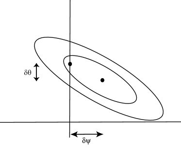
Figure 1: Illustrating how assumption of a wrong parameter value can influence the best-fitting value of other model parameters. Ellipses represent iso-likelihood surfaces, and here in the simpler model, the parameter on the horizontal axis is assumed to take the value given by the vertical line. Filled circles show the true parameters in the more complicated model, and the best-fit parameters in the simpler model.

If we assume that the posterior probability densities are small at the boundaries of the prior volume, then we can extend the integrations to infinity, and the integration over the multivariate Gaussians can be easily done. This gives, for $M$, $(2\pi)^{n/2}(\det{F})^{-1/2}$, so for nested models,

$$\langle B\rangle=(2\pi)^{-p/2}\frac{\sqrt{\det{F}}}{\sqrt{\det{F^{\prime}}}}\frac{L^{\prime}_{0}}{L_{0}}\Delta\theta_{n^{\prime}+1}\ldots\Delta\theta_{n^{\prime}+p}.$$ (10)

An equivalent expression was obtained, using again the Laplace approximation by Lazarides, Ruiz de Austri & Trotta (2004). The point here is that with the Laplace approximation, one can compute the $L^{\prime}_{0}/L_{0}$ ratio from the Fisher matrix. To compute this ratio of likelihoods, we need to take into account the fact that, if the true underlying model is $M$, in $M^{\prime}$ (the incorrect model), the maximum of the expected likelihood will not in general be at the correct values of the parameters (see Fig. 1). The $n^{\prime}$ parameters shift from their true values to compensate for the fact that, effectively, the $p$ additional parameters are being kept fixed at incorrect fiducial values. If in $M^{\prime}$, the additional $p$ parameters are assumed to be fixed at fiducial values which differ by $\delta\psi_{\alpha}$ from their true values, the others are shifted on average by an amount which is readily computed under the assumption of the multivariate Gaussian likelihood (see e.g. Taylor et al. (2007)):

$$\delta\theta^{\prime}_{\alpha}=-(F^{\prime-1})_{\alpha\beta}G_{\beta\zeta}\delta\psi_{\zeta}\qquad\alpha,\beta=1\ldots n^{\prime},\zeta=1\ldots p$$ (11)

where

$$G_{\beta\zeta}=\frac{1}{2}{\rm Tr}\left[C^{-1}C_{,\beta}C^{-1}C_{,\zeta}+C^{-1}(\mu_{,\zeta}\mu^{t}_{,\beta}+\mu_{,\beta}\mu^{t}_{,\zeta})\right],$$ (12)

which we recognise as a subset of the Fisher matrix. For clarity, we have given the additional parameters the symbol $\psi_{\zeta};\ \zeta=1\ldots p$ to distinguish them from the parameters in $M^{\prime}$.

With these offsets in the maximum likelihood parameters in model $M^{\prime}$, the ratio of likelihoods is given by

$$L^{\prime}_{0}=L_{0}\exp\left(-\frac{1}{2}\delta\theta_{\alpha}F_{\alpha\beta}\delta\theta_{\beta}\right)$$ (13)

where the offsets are given by $\delta\theta_{\alpha}=\delta\theta^{\prime}_{\alpha}$ for $\alpha\leq n^{\prime}$ (equation 11), and $\delta\theta_{\alpha}=\delta\psi_{\alpha-n^{\prime}}$ for $\alpha>n^{\prime}$.

The final expression for the expected Bayes factor is then

$$\langle B\rangle=(2\pi)^{-p/2}\frac{\sqrt{\det{F}}}{\sqrt{\det{F^{\prime}}}}\exp\left(-\frac{1}{2}\delta\theta_{\alpha}F_{\alpha\beta}\delta\theta_{\beta}\right)\prod_{q=1}^{p}\Delta\theta_{n^{\prime}+q}.$$ (14)

Note that $F$ and $F^{-1}$ are $n\times n$ matrices, $F^{\prime}$ is $n^{\prime}\times n^{\prime}$, and $G$ is an $n^{\prime}\times p$ block of the full $n\times n$ Fisher matrix $F$. The expression we find is a specific example of the Savage-Dickey ratio (Dickey (1971)); here we explicitly use the Laplace approximation to compute the offsets in the parameter estimates which accompany the wrong choice of model.

Note that the ‘Occam’s razor’ term, see Saini et al. (2004) for example, common in evidence calculations, is encapsulated in the $(2\pi)^{-p/2}\frac{\sqrt{\det{F}}}{\sqrt{\det{F^{\prime}}}}$ factor multiplied by the prior product: models with more parameters are penalised in favour of simpler models, unless the data demand otherwise. Such terms should be treated with caution, as pointed out by Linder & Miquel (2007) simpler models do not always result in the most physically realistic conclusions (but see Liddle et al. (2006) for a thorough discussion of the issues). In cases where the Laplace approximation is not a good one, other techniques must be used, at more computational expense (e.g. Trotta (2005, 2007); Beltran et al. (2005); Skilling (2004); Mukherjee, Parkinson & Liddle (2006); Parkinson, Mukherjee & Liddle (2006); Mukherjee et al. (2006)). Alternatively, a reparametrization of the parameter space can make the likelihood closer to gaussian (see e.g. Kosowsky et al. (2002) for CMB).

According to Jeffreys (1961), $1<\ln B<2.5$ is described as ‘substantial’ evidence in favour of a model, $2.5<\ln B<5$ is ‘strong’, and $\ln B>5$ is ‘decisive’. These descriptions seem too aggressive: $\ln B=1$ corresponds to a posterior probability for the less-favoured model which is 0.37 of the favoured model (Kass & Raftery (1995)). Other authors have introduced different terminology (e.g. Trotta (2005)).

3 Application: Dark Energy or Modified Gravity

To apply these results to cosmological probes of Dark Energy/modified gravity, we use the convenient Minimal Modified Gravity parametrization introduced by Linder (2005) and expanded by Linder & Cahn (2007) and Huterer & Linder (2006), where the beyond-Einstein perturbations are described by a growth factor $\gamma$. The growth rate of perturbations in the matter density $\rho_{m}$, $\delta\equiv\delta\rho_{m}/\rho_{m}$, is accurately parametrised as a function of scale factor $a(t)$ by

$$\frac{\delta}{a}\equiv g(a)=\exp\left\{\int_{0}^{a}\,\frac{da^{\prime}}{a^{\prime}}\left[\Omega_{m}(a^{\prime})^{\gamma}-1\right]\right\},$$ (15)

where $\Omega_{m}(a)$ is the density parameter of the matter. The growth factor $\gamma\simeq 0.55$ for the standard General Relativistic cosmological model, whereas for modified gravity theories it deviates from this value. For example, for the DGP braneworld model (Dvali, Gabadaze & Porrati (2000)), $\gamma\simeq 0.68$ (Linder & Cahn (2007)), on scales much smaller than those where cosmological acceleration is apparent. For this paper, we introduce $\gamma$ as an additional parameter in Model $M$ - i.e. $M$ represents extensions beyond General Relativity, whereas $M^{\prime}$ represents General Relativity with Dark Energy. Song, Hu, Sawicki (2007) show that the simplest flat DGP model demonstrates a difficulty pointed out by Ishak, Upadye & Spergel (2006), i.e. inconsistent parameter values are obtained from different datasets. Also the DGP model may be in difficulties with the CMB peak and baryon oscillations (Rydbeck, Fairbairn & Goobar (2007)), as well as theoretically through the existence of ghosts (Gorbunov, Koyama & Sibiryakov (2006)). Here we concentrate instead on distinguishing modified gravity models from GR using a different feature - that the growth factor is different from that of a quintessence model with the same expansion history. We use the DGP model as a specific example of a more general test of modified gravity models.

We make the (conservative) assumption that modification of gravity does not change the growth factor of perturbations on scales comparable to the horizon, i.e. in all cases the Integrated Sachs Wolfe (ISW) effect at large CMB angular scale is computed assuming the perturbation growth is given by standard gravity. In addition for the calculation of the CMB low $\ell$ multipoles we assume the dark energy perturbations associated to a scalar field with the same effective equation-of-state parameters as the modified gravity model. This is a conservative assumption as in a modified gravity model the ISW effect is expected to be different from standard gravity and therefore CMB observations may have some extra sensitivity to $\gamma$ which we ignore here.

The full set of parameters we explore in $M^{\prime}$ is $\Omega_{m},\Omega_{b},h,\sigma_{8},n_{s},\alpha_{n},\tau,r,w_{0},w_{a}$, being the density parameters in matter and baryons, the Hubble constant (in units of 100 km^-1Mpc^-1), the amplitude of fractional density perturbations, the primordial scalar spectral index of density fluctuations, and its running with wavenumber $k$, the reionisation optical depth, the tensor-to-scalar ratio; finally, there are two parameters characterising the expansion history of the Universe, $w(a)=w_{0}+w_{a}(1-a)$ (Chevallier & Polarski (2001)). For Dark Energy models, this is the equation of state parameter $p/(\rho c^{2})$ as a function of scale factor $a$. However, it is used here only as a means of parametrising of the expansion history, in terms of an effective Dark Energy component - $w(a)$ is not necessarily associated with a Dark Energy component. See Huterer & Linder (2006); Linder & Cahn (2007) and Kunz & Sapone (2006), For example, in the DGP model the expansion history is described well by $w_{0}=-0.78$, $w_{a}=0.32$. The Fisher matrices are almost unchanged if we take this as the fiducial model, so we present results for $w_{0}=-1$, $w_{a}=0$. $\gamma$ is an additional parameter in $M$ (set fixed at 0.55 in $M^{\prime}$), which parametrises the growth of structure For completeness, we list here the other fiducial parameters: $\Omega_{m}=0.27,\Omega_{b}=0.04,h=0.71,\sigma_{8}=0.8,n_{s}=1.0,\alpha_{n}=0.0,\tau=0.09,r=0.01$.

Thus the question we want to address is the following: assuming that the model of the Universe is a modified gravity model, is there an experimental setup which can distinguish this model from a Dark Energy model with the same expansion history? In this application we initially take the parameters of the model to be the DGP ones.

The experiments we consider are the upcoming Planck microwave background survey (Lamarre et al. (2003)), including polarisation information, three 3D weak lensing surveys and proposed SN and BAO surveys. Note that, as discussed above, we set the CMB constraint on $\gamma$ to zero. The constraint on $r$ and $\tau$ from the weak lensing is similarly zero - these are assumed fixed in the weak-lensing alone experiments; in the weak-lensing plus CMB, the constraints on $r$ and $\tau$ come from the CMB.

We consider a number of 3D weak lensing surveys: firstly a survey covering $5000$ square degrees to a median redshift of $z_{m}=0.8$ with a source density of $10$ galaxies per square arcminute, such as might be achieved with the Dark Energy Survey (DES) (Wester et al. (2005)); second a survey covering $30,000$ square degrees of the sky (Kaiser et al. (2002)) to a median depth of $z_{m}=0.75$ with $5$ galaxies per square arcminute, as might be achieved with Pan-STARRS (we consider only the single-telescope Pan-STARRS 1); third is a survey of $35$ sources per square arcminute, $z_{m}=0.90$, and an area of $20,000$ square degrees (next generation weak lensing survey, WL_NG), as might be observed by a space-based survey such as DUNE, which is a candidate for the ESA Cosmic Vision programme, or the Supernova Acceleration Probe (SNAP), a candidate of the NASA Joint Dark Energy Mission. Note that the characteristics of the Large Synoptic Survey Telescope (LSST) data set are not too dissimilar from these, so the reported numbers would be very close to those for LSST. For all surveys we assume flatness and a redshift dependence of source density $n(z)\propto z^{2}\exp\left[-(z/z*)^{1.5}\right]$, with $z*=1.4z_{m}$ and use the 3D weak shear power spectrum analysis method of Heavens (2003) and Heavens, Kitching & Taylor (2006). The modes are truncated at $k=1.5$Mpc^-1, avoiding the highly nonlinear regime where uncertainties in the power spectrum may lead to dominant systematic errors (Huterer & Linder (2006), Fig. 4).

The survey parameters are summarised in Table 1, including the photometric redshift error $\sigma_{z}$ and the number of sources per square arcminute, $n_{0}$. The Fisher matrices for the four experiments are available at http://www.roe.ac.uk/$\sim$afh. As there is a degeneracy between $w_{0}$, $w_{a}$ and $\gamma$ for Planck+WL, better constraints on the Universe expansion history lead to a better determination of $\gamma$ and therefore better model selection power. For probes of the expansion history we consider supernovae and a sample of $2000$ supernovae type 1a at $0<z\leq 1.8$ (see Virey et al. (2004) and Yeche et al. (2006)) as produced by SNAP (Aldering et al. (2004); Albert et al. (2005)) or the Advanced Dark Energy Probe Telescope (ADEPT, a candidate for the NASA Joint Dark Energy Mission; C. Bennett, private communication). For BAO we consider a wide survey contemplated by WFMOS (Bassett et al. (2005)) or ADEPT.

Survey	Area/sq deg	$z_{m}$	$n_{0}$/sq ’	$\sigma_{z}(z)$
DES	$5$,$000$	$0.80$	$10$	$0.05(1+z)$
PS1	$30$,$000$	$0.75$	$5$	$0.06(1+z)$
WLNG	$20$,$000$	$0.90$	$35$	$0.025(1+z)$

Table 1: The critical survey parameters for the Weak Lensing experiments considered. DES is the Dark Energy Survey, PS1 is the Pan-STARRS single telescope 3$\pi$ survey, and $WL_{NG}$ is a hypothetical ‘next-generation’ imaging survey, such as DUNE, SNAP, or LSST. $z_{m}$ is the median redshift, $n_{0}$ the number of sources per square arcminute, and $\sigma_{z}$ is the assumed photometric redshift error.

From these Fisher matrices (the Fisher matrix of a combination of independent data sets is the sum of the individual Fisher matrices), we compute the ratio of expected evidences assuming that the true model is a DGP braneworld, and take a prior range $\Delta\gamma=1$. Table 2 shows the expected evidence for the 3D weak lensing surveys with and without Planck.

We find that $\ln B$ obtained for the standard General Relativity model is only $\sim 1$ for DES+Planck, whereas for Pan-STARRS$+$Planck we find that $\ln B\sim 2$, for Pan-STARRS$+$Planck$+$SN$+$BAO $\ln B\sim 3.61$ and for WL_NG$+$Planck, $\ln B$ is a decisive $52.2$. Furthermore a WL_NG experiment could still decisively distinguish Dark Energy from modified gravity without Planck. The expected evidence in this case scales proportionally as the total number of galaxies in the survey. Pan-STARRS and Planck should be able to determine the expansion history, parametrised by $w(a)$ to very high accuracy in the context of the standard General Relativity cosmological model, with an accuracy of $0.03$ on $w(z\simeq 0.4)$, it will be able to substantially distinguish between General Relativity and the simplification of the DGP braneworld model considered here, although this does depend on there being a strong CMB prior.

The relatively low evidence from DES+Planck in comparison to Pan-STARRS+ Planck is due to the degeneracy between the running of the spectral index $\alpha$, and $\gamma$. The larger effect volume of Pan-STARRS, in comparison to DES, places a tighter constraint on this degeneracy. This could be improved by on-going high resolution CMB experiments.

Alternatively, we can ask the question of how different the growth rate of a modified-gravity model would have to be for these experiments to be able to distinguish the model from General Relativity, assuming that the expansion history in the modified gravity model is still well described by the $w_{0},w_{a}$ parametrization. This is shown in Fig.2. It shows how the expected evidence ratio changes with progressively greater differences from the General Relativistic growth rate. We see that a WL_NG survey could even distinguish ‘strongly’ $\delta\gamma=0.048$, Pan-STARRS $\delta\gamma=0.137$ and DES $\delta\gamma=0.179$. Note that changing the prior range $\Delta\gamma$ by a factor 10 changes the strong/decisive boundary for $\delta\gamma$ (for $WL_{NG}+$Planck) by $\sim 0.012$, so the dependence on the prior range is rather small.

If one prefers to ask a frequentist question, then a combination of WL_NG+Planck+BAO+SN should be able to distinguish $\delta\gamma=0.13$, at $10.6\sigma$. Results for other experiments are shown in Fig. 2.

Figure 2: The expected value of $|\ln B|$ from WL_NG (solid), Pan-STARRS (dot-dashed) and DES (dashed), in combination with CMB constraints from Planck, as a function of the difference in the growth rate between the modified-gravity model and General Relativity. The crossover at small $\delta\gamma$ occurs because Occam’s razor will favour the simpler (General Relativity) model unless the data demand otherwise. To the left of the cusps, GR would be likely to be preferred by the data. The dotted vertical line shows the offset of the growth factor for the DGP model. The horizontal lines mark the boundaries between ‘inconclusive’, ‘significant’, ‘strong’, and ‘decisive’ in Jeffreys’ (1961) terminology.

The case for a large, space-based 3D weak lensing survey is strengthened, as it offers the possibility of conclusively distinguishing Dark Energy from at least some modified gravity models.

Survey	$\nu$	$|\ln B|$
DES+Planck+BAO+SN	3.5	$1.28$	substantial
DES+Planck	2.2	$0.56$	inconclusive
DES	0.7	$0.54$	inconclusive
PS1+Planck+BAO+SN	2.9	$3.78$	strong
PS1+Planck	2.6	$2.04$	substantial
PS1	1.0	$0.62$	inconclusive
WLNG+Planck+BAO+SN	10.6	$63.0$	decisive
WLNG+Planck	10.2	$52.2$	decisive
WLNG	5.4	$11.8$	decisive

Table 2: The evidence ratio for the three weak lensing experiments considered with and without Planck, supernova and BAO priors. $WL_{NG}$ is a next-generation space-based imaging survey such as proposed for DUNE or SNAP. For completeness, we also list the frequentist significance $\nu\sigma$ with which GR would be expected to be ruled out, if the DGP braneworld were the correct model.

4 Conclusions

We have shown in this paper how one can compute the Bayesian Evidence under the assumption of a Gaussian likelihood surface, taking account of the fact that assuming the wrong model choice can affect the best-fitting values of parameters in the models. The assumption of a Gaussian likelihood is the same as used in the Fisher matrix approach to forecasting parameter errors, and we find that the Evidence can be calculated directly from the Fisher matrix alone, and with very little extra computation. An important caveat is that the assumption that the likelihood is a multivariate Gaussian is very strong, and deviations from this could easily change the evidence substantially. Nevertheless, the assumption is the same as is used in estimating marginal errors with Fisher matrices; for the CMB part used here we find agreement with 30% accuracy (note our Fisher matrices for Planck are conservative). However, this method should only be regarded as a first step, to identify which experimental setups are worth exploring with more detailed investigations. For the 3D weak lensing part of the study in particular, this method is extremely valuable, as simulating the surveys and subsequent analysis is an enormously time-consuming task.

We have also shown how future observations of the Cosmic Microwave Background, 3D weak lensing and probes of the expansion history of the Universe offer considerable promise of distinguishing decisively between Dark Energy models and modifications to General Relativity. In particular, a combination of Planck (CMB) and proposed space-based wide field imaging (weak lensing) surveys should be able decisively to distinguish a Dark Energy General Relativity model from a DGP modified-gravity model with natural log of the expected evidence ratio $\ln B\simeq 50$.

Surveys such as DUNE/SNAP/LSST, Pan-STARRS and DES, in combination with Planck, should be able to distinguish ‘strongly’ between General Relativity and minimally-modified gravity models with growth rates larger than 0.60, 0.69 and 0.73 respectively. The addition of probes of the expansion history of the Universe, such as supernova and baryon acoustic oscillation surveys help lift residual degeneracies and thus to distinguish ‘strongly’ models with growth rates larger than 0.59, 0.67 and 0.71 respectively.

References

- Albert et al. (2005) Albert J., et al., 2005, White paper to the Dark Energy Task Force, astroph/0507460
- Aldering et al. (2004) Aldering G. et al., 2004, “Supernova / Acceleration Probe: A Satellite Experiment to Study the Nature of the Dark Energy”, astroph/0405232
- Bassett et al. (2005) Bassett B., et al., 2005, A&G, 46e, 26
- Beltran et al. (2005) Beltran M., Garcia-Bellido J., Lesgourgues J., Liddle A. R., Slosar A., 2005, Phys, Rev., D71, 063532
- Bridges, Lasenby & Hobson (2006) Bridges M., Lasenby A. N., Hobson M. P. , 2006, MNRAS, 369, 1123
- Bridges, Lasenby & Hobson (2007) Bridges M., Lasenby A. N., Hobson M. P. , astro-ph/0607404
- Chevallier & Polarski (2001) Chevallier, Polarski D., 2001, JMPD, 10, 213
- Cornish N.J., Crowder J. (2005) Cornish N.J., Crowder J., 2005, Phys. Rev. D72, 043005
- Dickey (1971) Dickey J.M., 1971, Ann. Math. Stat., 42, 204
- Dvali, Gabadaze & Porrati (2000) Dvali G., Gabadaze G., Porrati M., 2000, Phys. Lett. B, 485, 208
- Eisenstein & Hu (1998) Eisenstein D. J., Wayne H., 1998, ApJ, 496, 605
- Fisher (1935) Fisher R.A., 1935, J. Roy. Stat. Soc., 98, 39
- Gorbunov, Koyama & Sibiryakov (2006) Gorbunov D., Koyama K., Sibiryakov S., (2006), Phys. Rev. D73, 4, 044016
- Heavens (2003) Heavens A.F., 2003, MNRAS, 343, 1327
- Heavens, Kitching & Taylor (2006) Heavens A.F., Kitching T.D., Taylor A.N., 2006, MNRAS, 373, 105
- Hobson, Bridle & Lahav (2002) Hobson M.P., Bridle S.L., Lahav O., 2002, MNRAS, 335, 377
- Hu (2002) Hu W., 2002, Phys. Rev. D, 65, 3003
- Huterer & Linder (2006) Huterer D., Linder E.V., 2006, astroph/0608681
- Ishak, Upadye & Spergel (2006) Ishak M., Upadye A., Spergel D.N., 2006, Phys Rev. D74, 4, 043513
- Jaffe (1996) Jaffe A., 1996, ApJ, 471, 24
- Jeffreys (1961) Jeffreys H., 1961, Theory of Probability, Oxford University Press (Oxford, UK)
- Kaiser et al. (2002) Kaiser N., et al., 2002, AAS, 20112207
- Kass & Raftery (1995) Kass R., Raftery A., 1995, J. Amer. Stat. Assoc., 90. 773
- Kosowsky et al. (2002) Kosowsky,A., Milosavljevic, M., Jimenez, R., 2002, Phys.Rev. D66 063007
- Kunz, Trotta & Parkinson (2006) Kunz M., Trotta R., Parkinson D., 2006, Phys. Rev. D, 74, 023503
- Kunz & Sapone (2006) Kunz M., Sapone D., 2006, astroph/0612452
- Lamarre et al. (2003) Lamarre J., et al., 2003, NewAR, 47, 1017
- Lazarides, Ruiz de Austri & Trotta (2004) Lazarides, G., Ruiz de Austri, R., Trotta, R., Phys. Rev. D70, 123527
- Liddle et al. (2006) Liddle A., Mukherjee P., Parkinson D., Wang Y., 2006, astroph/0610126
- Liddle et al. (2006) Liddle A., Corasaniti P. S., Kunz M., Mukherjee P., Parkinson D., Trotta R., 2007, astroph/0703285
- Linder (2005) Linder E.V., 2005, Phys. Rev. D, 72, 043529
- Linder & Cahn (2007) Linder E.V., Cahn R.N. 2007, astroph/0701317
- Linder & Miquel (2007) Linder E.V., Miquel, R., 2007, astroph/0702542
- Lucy & Sweeney (1971) Lucy L.B., Sweeney M.A., 1971, AJ, 76, 544
- Mukherjee, Parkinson & Liddle (2006) Mukherjee P., Parkinson D., Liddle A.R., 2006, ApJ, 638, L51
- Mukherjee et al. (2006) Mukherjee, P., Parkinson,D., Corasaniti, P. S., Liddle, A. R., Kunz, M., 2006, MNRAS, 369, 1725
- Parkinson, Mukherjee & Liddle (2006) Parkinson D.,Mukherjee P., Liddle A.R., 2006, Phys.Rev. D73, 123523
- Pahud et al. (2006) Pahud C., Liddle A., Mukherjee P., Parkinson D., 2006, Phys. Rev. D73, 123524
- Pahud et al. (2007) Pahud C., Liddle A., Mukherjee P., Parkinson D., 2007, astroph/0701481
- Peebles & Ratra (1988) Peebles P.J.E., Ratra B., 1988, ApJ, 325, L17
- Riess et al. (1998) Riess A., et al., 1998, AJ, 116, 1009
- Rydbeck, Fairbairn & Goobar (2007) Rydbeck S., Fairbairn M., Goobar A., (2007), astroph/0701495
- Saini et al. (2004) Saini T.D., Weller J., Bridle S.L., 2004, MNRAS, 348, 603
- Serra, Heavens & Melchiorri (2007) Serra P., Heavens A.F., Melchiorri A., 2007, astroph/0701338
-
Skilling (2004)
Skilling J., 2004, avaliable at
http://www.inference.phy.cam.ac.uk/bayesys - Song, Hu, Sawicki (2007) Song Y.-S., Hu W., Sawicki I., 2007, Phys. Rev. D75, 4, 044004
- Szydlowski & Godlowski (2006a) Szydlowski M., Godlowski W., 2006a, Phys. Lett. B633, 427
- Szydlowski & Godlowski (2006b) Szydlowski M., Godlowski W., 2006b, Phys. Lett. B639, 5
- Taylor et al. (2007) Taylor A.N., Kitching T.D., Bacon D.J., Heavens A.F., 2007, MNRAS, in press, (astroph/0606416)
- Tegmark, Taylor & Heavens (1997) Tegmark M., Taylor A.N., Heavens A.F., 1997, ApJ, 480, 22
- Trotta (2005) Trotta R., 2005, astroph/0504022
- Trotta (2006) Trotta R., 2006, To appear in ‘Cosmology, galaxy formation and astroparticle physics on the pathway to the SKA’, Oxford, (astroph/0607496)
- Trotta (2007) Trotta R., 2007, astroph/0703063
- Virey et al. (2004) Virey J., et al., 2004, PhRvD, 70, l1301
- Wang et al. (2004) Wang Y., Kratoshvil J.M., Linde A., Shmakova M., 2004, JCAP 12, 6
- Wester et al. (2005) Wester W., 2005, ASPC, 339, 152
- Wetterlich (1988) Wetterlich C., 1988, Nuc. Phys. B, 302, 668
- Yeche et al. (2006) Yeche C., et al., 2006, A&A, 448, 831