3D Relativistic Magnetohydrodynamic Simulations of Magnetized Spine-Sheath Relativistic Jets

Abstract

Numerical simulations of weakly magnetized and strongly magnetized relativistic jets embedded in a weakly magnetized and strongly magnetized stationary or weakly relativistic ($v=c/2$) sheath have been performed. A magnetic field parallel to the flow is used in these simulations performed by the new GRMHD numerical code RAISHIN used in its RMHD configuration. In the numerical simulations the Lorentz factor $\gamma=2.5$ jet is precessed to break the initial equilibrium configuration. In the simulations sound speeds are $\lesssim c/\sqrt{3}$ in the weakly magnetized simulations and $\lesssim 0.3~{}c$ in the strongly magnetized simulations. The Alfvén wave speed is $\lesssim 0.07~{}c$ in the weakly magnetized simulations and $\lesssim 0.56~{}c$ in the strongly magnetized simulations. The results of the numerical simulations are compared to theoretical predictions from a normal mode analysis of the linearized relativistic magnetohydrodynamic (RMHD) equations capable of describing a uniform axially magnetized cylindrical relativistic jet embedded in a uniform axially magnetized relativistically moving sheath. The theoretical dispersion relation allows investigation of effects associated with maximum possible sound speeds, Alfvén wave speeds near light speed and relativistic sheath speeds. The prediction of increased stability of the weakly magnetized system resulting from $c/2$ sheath speeds and the stabilization of the strongly magnetized system resulting from $c/2$ sheath speeds is verified by the numerical simulation results.

1 Introduction

Relativistic jets are associated with galaxies and quasars (AGN), with black hole binary star systems, and are thought responsible for the gamma-ray bursts (GRBs). In AGN and microquasar jets proper motions of intensity enhancements indicate motions that are mildly superluminal for the microquasar jets $\sim 1.2~{}c$ (Mirabel & Rodriquez 1999), and range from subluminal ($\ll c$) to superluminal ($\lesssim 6~{}c$) along the M 87 jet (Biretta et al. 1995, 1999), up to $\sim 25~{}c$ along the 3C 345 jet (Zensus et al. 1995; Steffen et al. 1995), and have inferred Lorentz factors $\gamma>100$ in the GRBs (e.g., Piran 2005). The various observed proper motions along AGN and microquasar jets imply speeds from $\sim 0.9~{}c$ up to $\sim 0.999~{}c$, and the inferred speeds for the GRBs are $\sim 0.99999~{}c$.

Jets at the larger scales may be kinetically dominated and contain relatively weak magnetic fields, e.g., equipartition between magnetic and gas pressure or less, but the possibility of much stronger magnetic fields certainly exists closer to the acceleration and collimation region. Here general relativistic magnetohydrodynamic (GRMHD) simulations of jet formation (e.g., Koide et al. 1998, 1999, 2000; Nishikawa et al. 2005; De Villiers et al. 2003, 2005; Hawley & Krolik 2006; McKinney & Gammie 2004; McKinney 2006; Mizuno et al. 2006b) and earlier theoretical work (e.g., Lovelace 1976; Blandford 1976; Blandford & Znajek 1977; Blandford & Payne 1982) invoke strong magnetic fields. Additionally, Vlahakis and Konigl have argued that magnetically dominated “Poynting flux” jets could produce the accelerations observed in AGN jets such as that in NGC 6251 and 3C 345 (Vlahakis & Konigl 2004) or provide the impetus for high Lorentz factor gamma-ray bursts outflows (Vlahakis & Konigl 2003). In these cases acceleration occurs up to the point at which Poynting fluxes and kinetic energy fluxes become comparable. In addition to strong magnetic fields, a number of GRMHD simulation studies of jet formation indicate that highly collimated high speed jets driven by the magnetic fields threading the ergosphere may themselves reside within a broader wind or sheath outflow driven by the magnetic fields anchored in the accretion disk (e.g., McKinney 2006; Hawley & Krolik 2006; Mizuno et al. 2006b). This configuration might additionally be surrounded by a less collimated accretion disk wind from the hot corona (e.g., Nishikawa et al. 2005).

Recent observations of high speed winds in several QSO’s with speeds, $\sim 0.1-0.4c$, also indicate that a highly relativistic jet could reside in a high speed wind or sheath, at least close to the central engine (Chartas et al. 2002, 2003; Pounds et al. 2003a, 2003b; Reeves et al. 2003). For some time other observational evidence such as limb brightening has been interpreted as evidence for a slower external flow surrounding a faster jet spine, e.g., Mkn 501 (Giroletti et al. 2004), M 87 (Perlman et al. 2001), and a few other radio galaxy jets (e.g., Swain et al. 1998; Giovannini et al. 2001). Additional circumstantial evidence such as the requirement for large Lorentz factors suggested by the TeV BL Lacs when contrasted with much slower observed motions has been used to suggest the presence of a spine-sheath morphology (Ghisellini et al. 2005). Siemignowska et al. (2006) have proposed a two component (spine-sheath) model to explain the broad-band emission from the PKS 1127-145 jet. Additionally, a spine-sheath jet structure has been proposed based on theoretical arguments (e.g., Sol et al. 1989; Henri & Pelletier 1991; Laing 1996; Meier 2003) and similar type structure has been investigated in the context of GRB jets (e.g., Rossi et al. 2002; Lazzatti & Begelman 2005; Zhang et al. 2003, 2004; Morsony et al. 2006).

In most jet generation numerical and theoretical work it has been necessary to assume an axisymmetric configuration. Given the helicity in the real system, e.g., helical magnetic field or outwards flow combined with rotation, there exists a potential problem with the stability of the system. Obviously, at least for most AGN jets, stability problems are surmounted and a highly collimated relatively stable flow is produced. In this paper we begin a 3D numerical study of the stability properties of highly relativistic jet flows allowing for the effects of strong magnetic fields and relativistic flow in a sheath around the highly relativistic jet. We note that observed relatively stable jet flow along with observed jet structures might then be used to constrain the configuration in the acceleration and collimation region where magnetic field strengths are high.

In the past, 3D numerical simulations of relativistic unmagnetized jets along with accompanying theoretical work (e.g., Hardee et al. 2001; Agudo et al. 2001; Hardee & Hughes 2003) has provided relatively unambiguous interpretation and understanding of structures observed in the numerical simulations. Thus, we begin our study by adopting a simple system, no radial dependence of quantities inside the jet and also no radial dependence of quantities outside the jet. This “top hat” configuration can be described exactly by the linearized RMHD equations. In general, the system consisting of a jet with “top hat” profile and magnetic field parallel to the flow along with a uniform external medium also with magnetic field parallel to the flow is more stable than a system with magnetic and flow helicity. Such a system is stable to current driven (CD) modes of instability (Istomin & Pariev 1994, 1996; Lyubarskii 1999) but can be unstable to Kelvin-Helmholtz (KH) modes of instability (Hardee 2004). This approach allows us to look at the potential KH modes without complications arising from coexisting CD modes (see Baty et al. 2004)

This paper is organized as follows. In section 2, we describe the numerical simulation setup and present the results of the three-dimensional RMHD simulations of spine-sheath relativistic jets. In section 3, we present the theoretical dispersion relation that arises from a normal mode analysis of the linearized RMHD equations, present relevant analytical approximate solutions, numerically solve the dispersion relation for the simulation parameters and compare to the simulation results. In section 4 we conclude.

2 Numerical Simulations of Spine-Sheath Jets

2.1 Numerical Method

In order to study the long-term stability of magnetized sheath-spine relativistic jets, we use the 3-dimensional GRMHD code “RAISHIN” with Cartesian coordinates in special relativity. The method is based on a 3+1 formalism of the general relativistic conservation laws of particle number and energy momentum, Maxwell equations, and Ohm’s law with no electrical resistance (ideal MHD condition) in a curved spacetime (Mizuno et al. 2006a). The RAISHIN code performs special relativistic calculations in Minkowski spacetime by changing the metric.

In the RAISHIN code, a conservative, high-resolution shock-capturing scheme is employed. The numerical fluxes are calculated using the Harten, Lax, & van Leer (HLL) approximate Riemann solver scheme. The flux-interpolated, constrained transport scheme is used to maintain a divergence-free magnetic field. The RAISHIN code has proven to be accurate to second order and has passed a number of numerical tests including highly relativistic cases, and highly magnetized cases in both special and general relativity (Mizuno et al. 2006a).

In the simulations a “preexisting” jet flow is established across the computational domain. This setup represents the case in which the jet is in equilibrium with an external medium far behind the leading edge Mach disk and bow shock. We allow the jet flow to be surrounded by a lower-density external magnetized wind medium. For all simulations, the ratio of densities is $\rho_{j}/\rho_{e}=2.0$, where $\rho$ is the mass density in the proper frame. The jet flow has $u_{j}=0.9165c$ and $\gamma\equiv(1-u^{2})^{-1/2}=2.5$. The initial magnetic field is assumed to be uniform and parallel to the jet flow. The jet is established in static total pressure balance with the external magnetized wind medium. Our choice of colder jet in a hotter wind is representative of a jet spine in a hotter sheath or cocoon as might occur as a result of astrophysical jet interaction with the surrounding medium. However, the specific parameters have been chosen for numerical and theoretical comparison convenience.

The computational domain is $6R_{j}\times 6R_{j}\times 60R_{j}$ with $60\times 60\times 600$ computational zones (10 computational zones span $R_{j}$). We impose outflow boundary conditions on all surfaces except the inflow plane at $z=0$.

A precessional perturbation is applied at the inflow by imposing a transverse component of velocity with $u_{\bot}=0.01u_{j}$. Simulations have been performed with precessional perturbations of angular frequency $\omega R_{j}/u_{j}=0.40$ (simulation A, $\omega 1$), $0.93$ (simulation B, $\omega 2$) and $2.69$ (simulation C, $\omega 3$). The simulations are halted after $\sim 60$ light crossing times of the jet radius, before the perturbation has crossed the entire computational domain.

We have performed two sets of simulations. RHD cases are weakly magnetized (see Table 1). The relevant sound speeds are $a_{e}=0.574c$ and $a_{j}=0.511c$, where the sound speed $a$ is given by

$$a\equiv\left[{\Gamma p\over\rho+(\Gamma/\Gamma-1)(p/c^{2})}\right]^{1/2}~{},$$ (1)

with $\Gamma=13/6$ as the adiabatic index appropriate to a mixture of relativistically hot electrons and cold baryons (Synge 1957). The relevant Alfvén speeds are $v_{Ae}=0.0682c$ and $v_{Aj}=0.064c$ , where the Alfvén speed $v_{A}$ is given by

$$v_{A}\equiv\left[{B^{2}\over\rho+(\Gamma/\Gamma-1)(p/c^{2})+B^{2}}\right]^{1/2}~{}.$$ (2)

Therefore the Alfvén speed is much smaller than sound speed. RMHD cases are strongly magnetized (see Table 1). The relevant sound speeds are $a_{e}=0.30c$ and $a_{j}=0.226c$. The relevant Alfvén speeds are $v_{Ae}=0.56c$ and $v_{Aj}=0.45c$. In this case the Alfvén speeds are approximately twice the sound speeds. In order to investigate the effect of an external wind, we have performed a no wind case ($u_{e}=0$, simulation ‘n’) and a mildly relativistic wind case ($u_{e}=0.5~{}c$, simulation ‘w’).

2.2 Numerical Results

Figure 1: Three-dimensional isovolume image (panels a, d) and two-dimensional axial (panels b, e) and transverse (panels c, f) slices made at $z=30R_{j}$ and simulation time $t=60$ for the weakly magnetized cases with precession frequency $\omega=0.93$. Panels a, b & c are for no wind (RHDBn) and panels d, e & f are with a wind (RHDBw). The colors show the logarithm of density, white lines indicate magnetic field lines (a, d), and arrows depict transverse velocities.

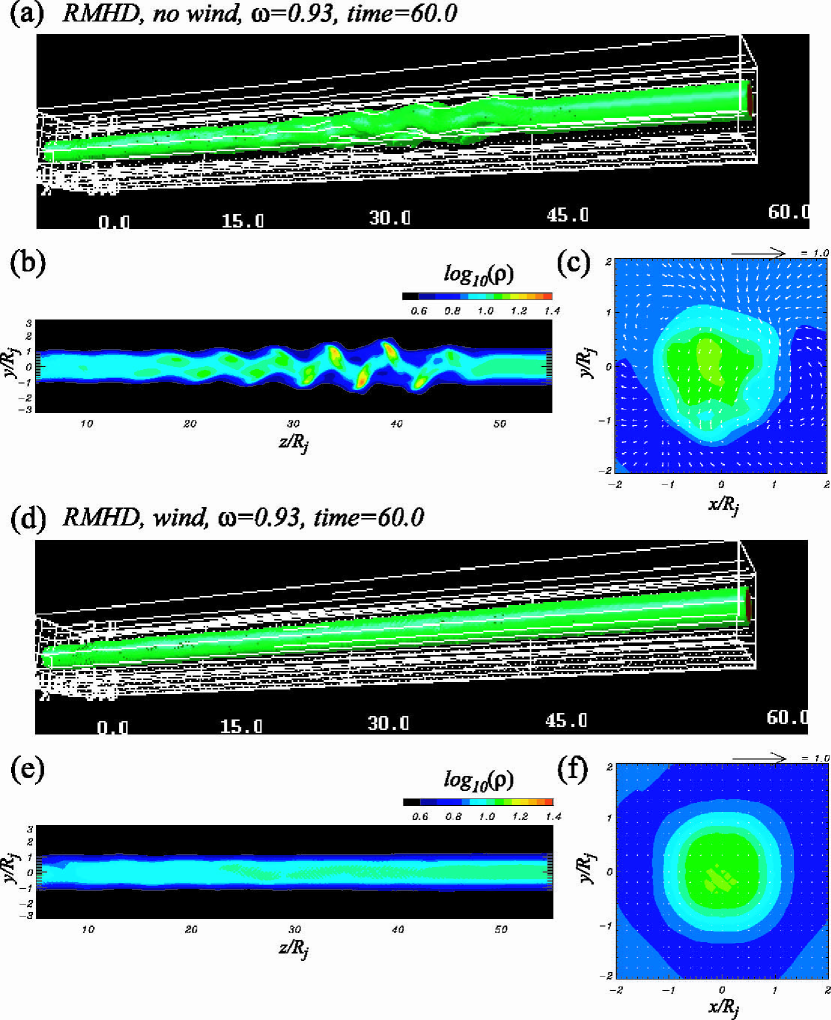
Figure 2: Three-dimensional isovolume image (panels a, d) and two-dimensional axial (panels b, e) and transverse (panels c, f) slices made at $z=30R_{j}$ and simulation time $t=60$ for the strongly magnetized cases with precession frequency $\omega=0.93$. Panels a, b & c are for no wind (RMHDBn) and panels d, e & f are with a wind (RMHDBw). The colors show the logarithm of density, white lines indicate magnetic field lines (a, d)and arrows depicts transverse velocities.

Figure 1 illustrates the difference in jet structure for weak magnetization with no wind and with an external wind. Specifically we show results from the intermediate precession frequency, $\omega 2\equiv\omega R_{j}/u_{j}=0.93$, (cases RHDBn and RHDBw) at simulation time $t=60$. Precession at the jet inflow plane excites the helical KH mode which is advected down the jet and grows. The isovolume image shows that beyond $z\sim 30R_{j}$ with no wind jet flow is disrupted, and the magnetic field is strongly bent and distorted. Transverse 2D slices through the jet axis (panels 1b & 1c) show a smaller density (pressure) fluctuation associated with the leading edge of the helix in the presence of the external wind. Transverse 2D slices perpendicular to the jet axis at $z=30R_{j}$ (panels 1c & 1f), suggest a less distorted jet in the presence of the external wind. Transverse velocities shown by the arrows indicate a circulation around the jet associated with the helical twist that is much more regular in the presence of the external wind.

Figure 2 illustrates jet structure for the strongly magnetized cases with no wind and with an external wind. As in Figure 1 we show results for the intermediate precession frequency, $\omega 2$, (cases RMHDBn and RMHDBw) at simulation time $t=60$. In the no wind case the helical KH mode grows but more slowly than in the weakly magnetized cases shown in Figure 1 and does not disrupt the jet inside $z\sim 40R_{j}$. A weakly twisted helical flow and magnetic structure develops. The transverse slice at $z=30R_{j}$ (panel 2c) indicates weak interaction between the jet and the external medium at this distance. Some circular circulation is seen. In the strongly magnetized case with the external wind (RMHDBw), the helical KH mode is damped and can just barely be seen out to $z=35R_{j}$ in the transverse axial slice (panel 2e). The transverse slice at $z=30R_{j}$ indicates negligible interaction between jet and external medium and no circular circulation (panel 2f).

It is immediately clear from Figure 1 that presence of the wind provides a stabilizing influence in the weakly magnetized case. Further comparison with Figure 2 shows that the presence of a strong magnetic field provides a stabilizing influence and complete stabilization in the presence of the strongly magnetized wind.

To investigate simulation results quantitatively, we take one-dimensional cuts through the computational box parallel to the z-axis at radial distances $x/R_{j}=0.2$, $0.5$, and $0.8$ on the transverse x-axis. The results for weakly magnetized cases with/without the external wind are shown in Figures 3, 4, & 5 for precession frequencies, $\omega R_{j}/u_{j}=0.4,~{}0.93,~{}\&~{}2.69$ respectively. The results for the strongly magnetized cases are shown in Figures 6 & 7 for precession frequencies $\omega R_{j}/u_{j}=0.93,~{}\&~{}2.69$ respectively. In the figures, $u_{x}$ and $u_{y}$ velocity components correspond to radial $u_{r}$ and azimuthal $u_{\phi}$ velocity components in cylindrical geometry.

In the weakly magnetized cases oscillation from the growing helical KH mode is seen in all cases. From the plots of radial and transverse velocities, the dominant wavelengths of oscillation are $\lambda/R_{j}\sim 13,~{}6,~{}\&~{}2$ for low, intermediate, and high frequency precession with no wind and with a measurable lengthening to $\lambda/R_{j}\sim 14$ for low frequency precession with the wind. For the high-frequency case without the external wind, the azimuthal velocity component suggests a beat pattern with wavelength, $\lambda^{n}_{beat}(\omega 3)\lesssim 20R_{j}$. From the axial velocities near the jet axis, we see that jet flow is disrupted at $z\sim 25R_{j}$, $z\sim 32R_{j}$, and possibly for $z\gtrsim 50R_{j}$ for the low, intermediate and high precession frequency no wind cases respectively. Jet flow is disrupted at $z\sim 43R_{j}$, $z\sim 35R_{j}$ and possibly for $z\gtrsim 50R_{j}$ for the low, intermediate and high frequency precession wind cases respectively. Thus, the external wind reduces the growth of KH instability and delays the onset of flow disruption. The large dips in the axial velocity near the jet surface are caused by sideways motion of the jet surface. Dips in the axial velocity occur more deeply inside the jet surface for lower frequency precession. The presence of the external wind reduces these effects somewhat.

Quantitative simulation results for the strongly magnetized cases with/without the external wind are shown in Figures 6 and 7. In the absence of the external wind (RMHDBn and RMHDCn) growing oscillation from helical KH instability is seen. However, spatial growth is much slower than for the comparable weakly magnetized cases. Comparison with the weakly-magnetized cases (RHDBn and RHDCn), shows that the magnetic field reduces the growth rate of KH instabilities such that any disruption of collimated flow will lie at $z\gg 40R_{j}$. In the presence of the external wind (RMHDBw and RMHDCw) the initial oscillation is damped. Damping is more rapid for the intermediate frequency perturbation than for the high frequency perturbation. Plots of radial and transverse velocities, and the radial magnetic field component shown in one-dimensional cuts in Figures 6 and 7 show that the dominant wavelengths of oscillation are $\lambda/R_{j}\sim 5~{}\&~{}2$ for the intermediate and high frequency perturbations, respectively with or without the external wind. There is a possible beat pattern in the azimuthal velocity component with $\lambda^{mn}_{beat}(\omega 2)\sim 10~{}R_{j}$ for $z<20~{}R_{j}$ in the no wind high frequency case. The presence of the wind results in more readily seen beat patterns accompanying the damped oscillations. The beat pattern is best seen in the radial magnetic field amplitude (Fig. 6f and Fig. 7f). At the intermediate perturbation frequency the beat wavelength is $\lambda^{mw}_{beat}(\omega 2)\gtrsim 20~{}R_{j}$. In the high-frequency case a clear beat pattern with $\lambda^{mw}_{beat}(\omega 3)\sim 10~{}R_{j}$ is seen at $z<33~{}R_{j}$ but disappears at larger $z$.

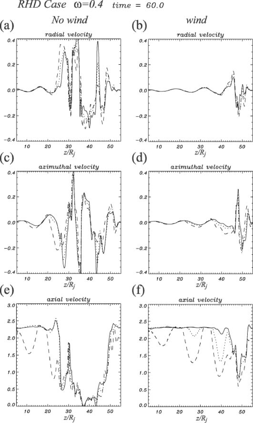
Figure 3: Radial velocity ($u_{x}$), azimuthal velocity ($u_{y}$), and axial velocity ($\gamma u_{z}$) along the one-dimensional cuts parallel to the jet axis located at $x/R_{j}=0.2$(solid line), $0.5$(dotted line) and $0.8$(dashed line) for low-frequency precession of a weakly magnetized jet for no wind (RHDAn)(left panels) and with an external wind (RHDAw)(right panels).

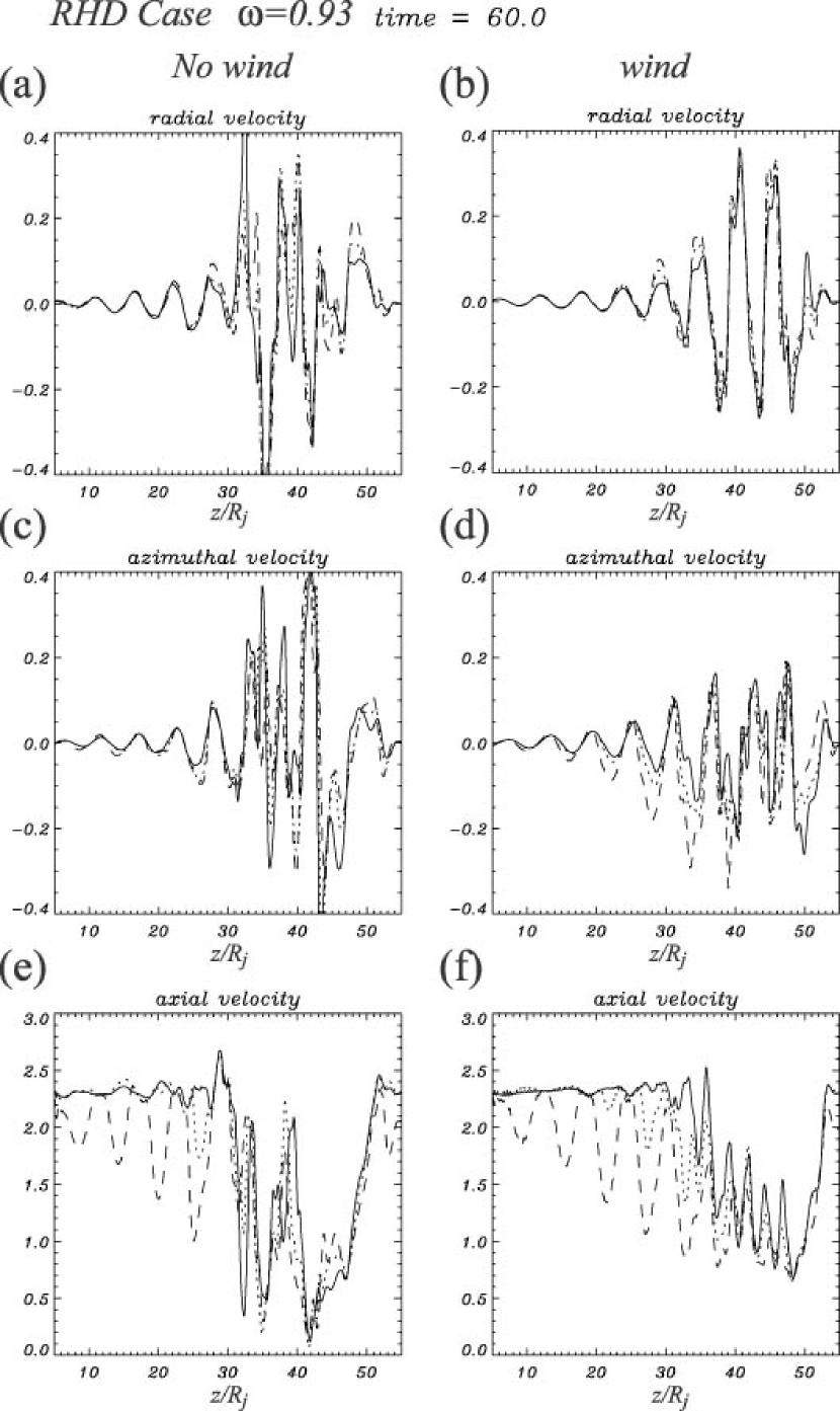
Figure 4: Radial velocity ($u_{x}$), azimuthal velocity ($u_{y}$), and axial velocity ($\gamma u_{z}$) along the one-dimensional cuts parallel to the jet axis located at $x/R_{j}=0.2$(solid line), $0.5$(dotted line) and $0.8$(dashed line) for intermediate frequency precession of a weakly magnetized jet for no wind (RHDBn)(left panels) and with an external wind (RHDBw)(right panels).

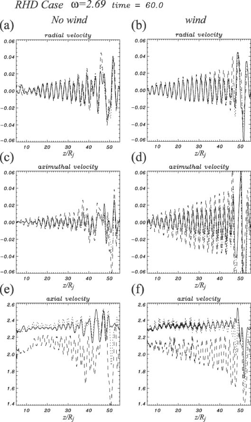
Figure 5: Radial velocity ($u_{x}$), azimuthal velocity ($u_{y}$), and axial velocity ($\gamma u_{z}$) along the one-dimensional cuts parallel to the jet axis located at $x/R_{j}=0.2$(solid line), $0.5$(dotted line) and $0.8$(dashed line) for high frequency precession of a weakly magnetized jet for no wind (RHDCn)(left panels) and with an external wind (RHDCw)(right panels).

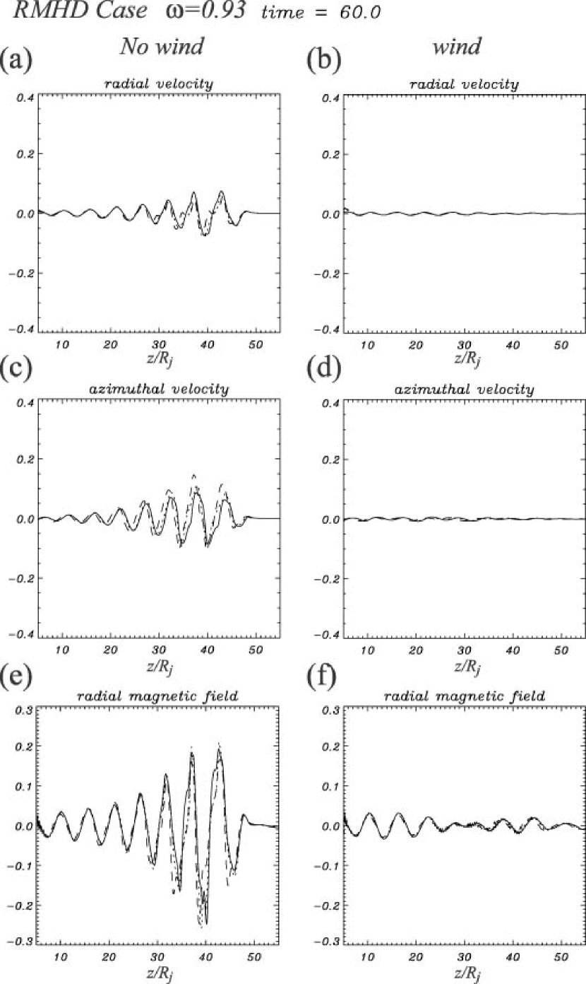
Figure 6: Radial velocity ($u_{x}$), azimuthal velocity ($u_{y}$), and radial magnetic field ($B_{x}$) along the one-dimensional cuts parallel to the jet axis located at $x/R_{j}=0.2$(solid line), $0.5$(dotted line) and $0.8$(dashed line) for intermediate frequency precession of a strongly magnetized jet for no wind (RMHDBn)(left panels) and with a strongly magnetized external wind (RMHDBw)(right panels).

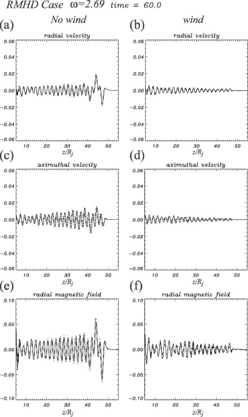
Figure 7: Radial velocity ($u_{x}$), azimuthal velocity ($u_{y}$), and radial magnetic field ($B_{x}$) along the one-dimensional cuts parallel to the jet axis located at $x/R_{j}=0.2$(solid line), $0.5$(dotted line) and $0.8$(dashed line) for high frequency precession of a strongly magnetized jet for no wind (RMHDCn) (left panels) and with a strongly magnetized external wind (RMHDCw)(right panels).

In the next section we will compare these simulation results with theoretical predictions for growth and damping of the helical wave mode excited by the inlet perturbations in our numerical simulations.

3 Theory and Analysis

3.1 Dispersion Relation

Stability of a jet spine-sheath or jet-wind configuration, where the sheath or wind is much broader than the spine or jet, can be accomplished by modeling the jet/spine as a cylinder of radius R embedded in an infinite wind/sheath.

Formally, the assumption of an infinite sheath means that the analysis could be performed in the reference frame of the sheath and numerical simulations could be performed in the reference frame of the sheath with results transformed to the source/observer reference frame. However, it is not much more difficult to derive a dispersion relation and obtain analytical expressions in the source/observer frame and analytical solutions to the dispersion relation in the source/observer frame take on simple physically revealing forms (Hardee 2007). Additionally, this approach lends itself to modeling the propagation and appearance of jet structures viewed in the source/observer frame, e.g., helical structures in the 3C 120 jet (Hardee et al. 2005).

A dispersion relation describing the growth or damping of the normal wave modes associated with this system can be derived if uniform conditions are assumed within the jet/spine, e.g., having a uniform proper density, $\rho_{j}$, a uniform axial magnetic field, $B_{j}=B_{j,z}$, and a uniform velocity, $\mathbf{u}_{j}=u_{j,z}$, and if uniform conditions are assumed within the external sheath/wind, e.g., having a uniform proper density, $\rho_{e}$, a uniform axial magnetic field, $B_{e}=B_{e,z}$, and a uniform velocity $\mathbf{u}_{e}=u_{e,z}$. Here the jet/spine is established in static total pressure balance with the external wind/sheath where the total static uniform pressure is $P_{e}^{\ast}\equiv P_{e}+B_{e}^{2}/8\pi=P_{j}^{\ast}\equiv P_{j}+B_{j}^{2}/8\pi$.

The dispersion relation is obtained from the linearized ideal RMHD and Maxwell equations, where the density, velocity, pressure and magnetic field are written as $\rho=\rho_{0}+\rho_{1}$, $\mathbf{v}=\mathbf{u}+\mathbf{v}_{1}$ (we use $\mathbf{v}_{0}\equiv\mathbf{u}$ for notational reasons), $P=P_{0}+P_{1}$, and $\mathbf{B}=\mathbf{B}_{0}+\mathbf{B}_{1}$, where subscript 1 refers to a perturbation to the equilibrium quantity with subscript 0. Additionally, the Lorentz factor $\gamma^{2}=(\gamma_{0}+\gamma_{1})^{2}\simeq\gamma_{0}^{2}+2\gamma_{0}^{4}\mathbf{u\cdot v}_{1}/c^{2}$ where $\gamma_{1}=\gamma_{0}^{3}\mathbf{u\cdot v}_{1}/c^{2}$. It is assumed that the initial equilibrium system satisfies the zero order equations. Details of the derivation for the fully relativistic case can be found in Hardee (2007).

In cylindrical geometry a random perturbation $\rho_{1}$, $\mathbf{v}_{1}$ $\mathbf{B}_{1}$ and $P_{1}$ can be considered to consist of Fourier components of the form

$$f_{1}(r,\phi,z,t)=f_{1}(r)\exp[i(kz\pm n\phi-\omega t)]$$ (3)

where the zero order flow is along the z-axis, and r is in the radial direction with the jet/spine bounded by $r=R$. In cylindrical geometry $n$ is an integer azimuthal wavenumber, for $n>0$ waves propagate at an angle to the flow direction, and $+n$ and $-n$ give wave propagation in the clockwise and counter-clockwise sense, respectively, when viewed in the flow direction. In equation (1) $n=0$, $1$, $2$, $3$, $4$, etc. correspond to pinching, helical, elliptical, triangular, rectangular, etc. normal mode distortions of the jet, respectively. Propagation and growth or damping of the Fourier components can be described by a dispersion relation of the form

$$\frac{\beta_{j}}{\chi_{j}}\frac{J_{n}^{{}^{\prime}}(\beta_{j}R)}{J_{n}(\beta_{j}R)}=\frac{\beta_{e}}{\chi_{e}}\frac{H_{n}^{(1)^{\prime}}(\beta_{e}R)}{H_{n}^{(1)}(\beta_{e}R)}~{}.$$ (4)

In the dispersion relation $J_{n}$ and $H_{n}^{(1)}$ are Bessel and Hankel functions, and the primes denote derivatives of the Bessel and Hankel functions with respect to their arguments. In equation (4)

$$\chi_{j}\equiv\gamma_{j}^{2}\gamma_{Aj}^{2}W_{j}\left(\varpi_{j}^{2}-\kappa_{j}^{2}v_{Aj}^{2}\right)~{},$$ ()

$$\chi_{e}\equiv\gamma_{e}^{2}\gamma_{Ae}^{2}W_{e}\left(\varpi_{e}^{2}-\kappa_{e}^{2}v_{Ae}^{2}\right)~{},$$ ()

and

$$\beta_{j}^{2}\equiv\left[\frac{\gamma_{j}^{2}\left(\varpi_{j}^{2}-\kappa_{j}^{2}a_{j}^{2}\right)\left(\varpi_{j}^{2}-\kappa_{j}^{2}v_{Aj}^{2}\right)}{v_{msj}^{2}\varpi_{j}^{2}-\kappa_{j}^{2}v_{Aj}^{2}a_{j}^{2}}\right]~{},$$ ()

$$\beta_{e}^{2}\equiv\left[\frac{\gamma_{e}^{2}\left(\varpi_{ex}^{2}-\kappa_{e}^{2}a_{e}^{2}\right)\left(\varpi_{e}^{2}-\kappa_{e}^{2}v_{Ae}^{2}\right)}{v_{mse}^{2}\varpi_{e}^{2}-\kappa_{e}^{2}v_{Ae}^{2}a_{e}^{2}}\right]~{}.$$ ()

In equations (5a & 5b) and equations (6a & 6b) $\varpi_{j,e}^{2}\equiv\left(\omega-ku_{j,e}\right)^{2}$ and $\kappa_{j,e}^{2}\equiv\left(k-\omega u_{j,e}/c^{2}\right)^{2}$, $\gamma_{j,e}\equiv(1-u_{j,e}^{2}/c^{2})^{-1/2}$ is the flow Lorentz factor, $\gamma_{Aj,e}\equiv(1-v_{Aj,e}^{2}/c^{2})^{-1/2}$ is the Alfvén Lorentz factor, $W\equiv\rho+\left[\Gamma/\left(\Gamma-1\right)\right]P/c^{2}$ is the enthalpy, $a$ is the sound speed, $v_{A}$ is the Alfvén wave speed, and $v_{ms}$ is a magnetosonic speed. The sound speed is defined by

$$a\equiv\left[\frac{\Gamma P}{\rho+\left(\frac{\Gamma}{\Gamma-1}\right)P/c^{2}}\right]^{1/2}~{},$$

where $4/3\leq\Gamma\leq 5/3$ is the adiabatic index. The Alfvén wave speed defined by

$$v_{A}\equiv\left[\frac{V_{A}^{2}}{1+V_{A}^{2}/c^{2}}\right]^{1/2}$$

where $V_{A}^{2}\equiv B_{0}^{2}/(4\pi W_{0})$ is equivalent to equation (2). A magnetosonic speed corresponding to the fast magnetosonic speed for propagation perpendicular to the magnetic field (e.g., Vlahakis & Königl 2003) is defined by

$$v_{ms}\equiv\left[a^{2}+v_{A}^{2}-a^{2}v_{A}^{2}/c^{2}\right]^{1/2}=\left[a^{2}/\gamma_{A}^{2}+v_{A}^{2}\right]^{1/2}~{}.$$

Each normal mode $n$ contains a single fundamental wave ($\omega\rightarrow 0$, $k\rightarrow 0$, $\omega/k>0$) and multiple body wave($\omega\rightarrow 0$, $k>0$, $\omega/k\rightarrow 0$) solutions that satisfy the dispersion relation. In the numerical simulations the jet/spine was precessed in a manner designed to trigger the $n=1$ fundamental helical mode. Previous theoretical and simulation work has shown a sufficiently close coupling between fundamental and body modes that the simulation may excite the first body mode as well. In what follows here we consider the $n=1$ helical fundamental and first body mode solutions to the dispersion relation as being relevant to the numerical simulations performed here.

3.2 The Helical Mode

In the low frequency limit the helical fundamental mode has an analytic wave solution given by

$$\frac{\omega}{k}=\frac{\left[\eta u_{j}+u_{e}\right]\pm i\eta^{1/2}\left[\left(u_{j}-u_{e}\right)^{2}-V_{As}^{2}/\gamma_{j}^{2}\gamma_{e}^{2}\right]^{1/2}}{(1+V_{Ae}^{2}/\gamma_{e}^{2}c^{2})+\eta(1+V_{Aj}^{2}/\gamma_{j}^{2}c^{2})}$$ (7)

where $\eta\equiv\gamma_{j}^{2}W_{j}\left/\gamma_{e}^{2}W_{e}\right.$ and a “surface” Alfvén speed is given by

$$V_{As}^{2}\equiv\left(\gamma_{Aj}^{2}W_{j}+\gamma_{Ae}^{2}W_{e}\right)\frac{B_{j}^{2}+B_{e}^{2}}{4\pi W_{j}W_{e}}~{}.$$ (8)

In equation (8) note that the Alfvén Lorentz factor can be written as $\gamma_{Aj,e}^{2}=1+V_{Aj,e}^{2}/c^{2}$. The jet is predicted to be stable to the helical fundamental mode when

$$\left(u_{j}-u_{e}\right)^{2}-V_{As}^{2}/\gamma_{j}^{2}\gamma_{e}^{2}<0~{}.$$ (9)

Thus, as might be anticipated, the growth rate is directly related to the difference between the magnitude of a “shear” speed, $(u_{j}-u_{e})^{2}$, and a “surface” Alfvén speed. Note that the “surface” Alfvén speed can be greater than the speed of light and is not a physical wave speed. The growth rate is also reduced by the spine Lorentz factor through $\eta$ in the denominator of eq. (7). Finally, the real part of eq. (7) directly provides an estimate of the increase in helical pattern speed resulting from the external sheath flow, and this increase when combined with a decrease in the temporal growth rate implies an increase in the spatial growth length.

In the low frequency limit the real part of the first helical body wave solution has an analytic solution given approximately by

$$kR\approx k^{\min}R\equiv\frac{5}{4}\pi\left[\frac{v_{msj}^{2}u_{j}^{2}-v_{Aj}^{2}a_{j}^{2}}{\gamma_{j}^{2}(u_{j}^{2}-a_{j}^{2})(u_{j}^{2}-v_{Aj}^{2})}\right]^{1/2}~{}.$$ (10)

In this low frequency limit the body wave solution exists only when $k^{\min}R$ has a positive real part. This requires that

$$\left[\frac{v_{msj}^{2}u_{j}^{2}-v_{Aj}^{2}a_{j}^{2}}{\gamma_{j}^{2}(u_{j}^{2}-a_{j}^{2})(u_{j}^{2}-v_{Aj}^{2})}\right]>0~{}.$$ (11)

Thus, the first helical body mode exists when the jet is supersonic and super-Alfvénic, i.e., $u_{j}^{2}-a_{j}^{2}>0$ and $u_{j}^{2}-v_{Aj}^{2}>0$, or in a limited velocity range given approximately by $a_{j}^{2}>u_{j}^{2}>[\gamma_{sj}^{2}/(1+\gamma_{sj}^{2})]a_{j}^{2}$ when $v_{Aj}^{2}\approx a_{j}^{2}$, where $\gamma_{sj}\equiv(1-a_{j}^{2}/c^{2})^{-1/2}$ is a sonic Lorentz factor.

For a supermagnetosonic jet, the helical fundamental and first body modes can have a distinct maximum in the growth rate at some resonant frequency. The resonance condition can be evaluated analytically in either the fluid limit where $a\gg V_{A}$ or in the magnetic limit where $V_{A}\gg a$. Note that in the magnetic limit, magnetic pressure balance implies that $B_{j}=B_{e}$. In these cases a necessary condition for resonance is that

$$\frac{u_{j}-u_{e}}{1-u_{j}u_{e}/c^{2}}>\frac{v_{wj}+v_{we}}{1+v_{wj}v_{we}/c^{2}}~{},$$ (12)

where $v_{wj}\equiv\left(a_{j},v_{Aj}\right)$ and $v_{we}\equiv\left(a_{e},v_{Ae}\right)$ in the fluid or magnetic limits, respectively. This necessary condition for resonance indicates that we are supersonic or super-Alfvénic when the shear speed exceeds a physical “surface” wave speed. When this condition is satisfied it can be shown that the wave speed at resonance is

$$v_{w}\approx v_{w}^{\ast}\equiv\frac{\gamma_{j}(\gamma_{we}v_{we})u_{j}+\gamma_{e}(\gamma_{wj}v_{wj})u_{e}}{\gamma_{j}(\gamma_{we}v_{we})+\gamma_{e}(\gamma_{wj}v_{wj})}$$ (13)

where $\gamma_{w}\equiv(1-v_{w}^{2}/c^{2})^{-1/2}$ is the sonic or Alfvén Lorentz factor accompanying $v_{wj}\equiv\left(a_{j},v_{Aj}\right)$ and $v_{we}\equiv\left(a_{e},v_{Ae}\right)$ in the fluid or magnetic limits, respectively. The resonant wave speed and maximum growth rate occur at a frequency given by

$$\omega R/v_{we}\approx\omega_{m}^{\ast}R/v_{we}\equiv\frac{3\pi/4+m\pi}{\left[\left(1-u_{e}/v^{\ast}_{w}\right)^{2}-\left(v_{we}/v^{\ast}_{w}-u_{e}v_{we}/c^{2}\right)^{2}\right]^{1/2}}~{}.$$ (14)

In equation (14) $m=0,1$ specifies the fundamental and first body modes, respectively. A resonant wavelength is given by $\lambda\approx\lambda_{m}^{\ast}\equiv 2\pi v_{w}^{\ast}/\omega_{m}^{\ast}$ and can be calculated from

$$\lambda_{m}^{\ast}\equiv\frac{2\pi}{3\pi/4+m\pi}\left(\frac{\gamma_{e}}{v_{we}}\right)\left\{\left(v_{w}^{\ast}-u_{e}\right)^{2}-\left[v_{we}-(v_{we}u_{e}/c^{2})v_{w}^{\ast}\right]^{2}\right\}^{1/2}R~{}.$$ (15)

The resonant frequency is found to be largely a function of the sound and Alfvén wave speeds in the sheath and the shear speed, $u_{j}-u_{e}$ (Hardee 2007). The resonant frequency increases as the sound and Alfvén wave speeds increase and as the shear speed declines. In the limit

$$\frac{u_{j}-u_{e}}{1-u_{j}u_{e}/c^{2}}\longrightarrow\frac{v_{wj}+v_{we}}{1+v_{wj}v_{we}/c^{2}}~{},$$

the resonant frequency $\omega_{m}^{\ast}R/v_{we}\rightarrow\infty$. In general, When the sound or Alfvén wave speed increases relative to the jet speed there is an increase in the growth rate at the higher resonant frequency accompanying an increase in the sound or Alfvén wave speed relative to the jet speed. On the other hand, the growth rate at resonance decreases as the shear speed, $u_{j}-u_{e}$, declines. This decline in the growth rate is also indicated by equation (8) which applies to fundamental mode frequencies up to an order of magnitude below resonance. As the resonant frequency increases equation (8) applies to increasingly higher fundamental mode frequencies.

Numerical solution of the dispersion relation is necessary to obtain accurate values for growth or damping rates as fundamental mode frequencies approach and exceed the resonant frequency. In general, the behavior of growth or damping associated with the first body mode must be obtained by numerical solution of the dispersion relation at all frequencies. In the high frequency limit the real part of the fundamental and first body mode solutions to the dispersion relation tend towards the analytic limiting form

$$\frac{\omega}{k}\approx\frac{u_{j}\pm v_{wj}}{1\pm v_{wj}u_{j}/c^{2}}~{}.$$ (16)

which describes sound waves $v_{wj}=a_{j}$ or Alfvén waves $v_{wj}=v_{Aj}$ propagating with and against the jet flow inside the jet. Note that at high frequencies waves propagate in the spine fluid with speeds that are independent of the surrounding sheath and are decoupled from the spine sheath boundary.

3.3 Numerical Solution to the Dispersion Relation

In general, equations (7) and (10) provide initial estimates at low frequencies to the helical fundamental and first body mode solutions that can then be followed by root finding techniques to higher frequencies. The results of numerical solution to the dispersion relation for the parameters appropriate to the numerical simulations shown in section 2 are displayed in Figure 8. It should be noted that not all possible solutions are shown or have necessarily been found by the root finding technique. In general, in the weakly magnetized case fundamental (S) mode solutions consist of a growing (shown) and damped (not shown) solution pair with comparable growth and damping rates (see eq. 7) and first body (B1) mode solutions consist of a real and growing or damped solution pair. The presence of the external wind flow leads to reduced growth of the S mode and weak damping of the B1 mode.

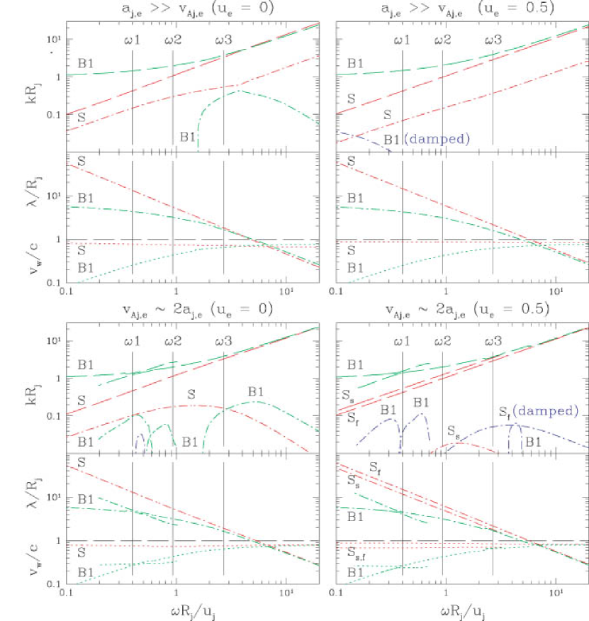
Figure 8: Solutions of the dispersion relation for helical fundamental (red lines) and first body (green lines) modes for weakly magnetized ($a_{j,e}\gg v_{Aj,e}$) and strongly magnetized ($a_{j,e}\sim v_{Aj,e}$) jet simulations without a surrounding outflow ($u_{e}=0$) and with a surrounding 0.5 c outflow ($u_{e}=0.5$). Dispersion relation solutions show the real, $k_{r}R_{j}$, (dashed lines) and imaginary, $k_{i}R_{j}$, (dash-dot lines) parts of the dimensionless wavenumber normalized by the jet radius, $R_{j}$, as a function of the dimensionless angular frequency, $\omega R_{j}/u_{j}$, normalized by the jet radius and jet speed, $u_{j}$. Where the imaginary part of the wavenumber is shown in blue, the solution is damped. Immediately under the panel showing a dispersion relation solution for fundamental (S) and first body (B1) modes is a panel that shows the wavelength, $\lambda/R_{j}$, (dash-dot lines) and wave speed, $v_{w}/c$, (dotted lines). The angular driving frequencies used in the numerical simulations are indicated by the vertical solid lines.

The solution structure is more complex in the strongly magnetized case. Comparable sound and Alfvén wave speeds have led to an increased complexity compared to the weakly magnetized case solutions or when compared to the analytically predicted results for Alfvén wave speed greatly exceeding the sound speed. In the absence of magnetized sheath flow S mode solutions again consist of a growing (shown) and damped (not shown) solution pair. Now however, we find multiple growing solutions associated with the B1 mode evident at the lower frequencies (see the lower left panel in Figure 8). A modest damping rate accompanies the crossing of the real part of these multiple body mode solutions. The complex structure of the first body mode solution shown in Figure 8 for the strongly magnetized cases has been seen previously in a non-relativistic stability analysis (see Figure 20 in Hardee et al. 1995). At the lowest frequencies, $\omega<\omega 1$, the first body mode consists of a solution pair whose real part can be identified with the descending and constant real part of the wavenumber. At frequencies above the crossing point, $\omega>\omega 1$, the rapidly rising real part of the wavenumber connects to the second body mode at a frequency $\omega>\omega 2$.

At the higher frequencies the B1 mode is similar to the weakly magnetized case. In the presence of magnetized sheath flow, there is significant difference in growth and damping rates for the S mode solution pair. Weak growth is associated with the slower, $S_{s}$, moving shorter wavelength solution and weak damping is associated with the faster, $S_{f}$, moving longer wavelength solution. At the intermediate frequency, $\omega 2$, and below the growth rate is larger than the damping rate but at the higher frequencies somewhat above $\omega 2$ the damping rate is larger than growth rate for the S mode solution pair. The presence of magnetized sheath flow leads to damping of the B1 mode at the lower frequencies where in the absence of magnetized sheath flow there was modest growth and a modest high frequency damping rate maximum is seen where B1 intersects $S_{s}$.

The wavelengths and growth/damping lengths normalized to the jet radius for the precession frequencies $\omega 1$, $\omega 2$ and $\omega 3$ used in the weakly magnetized simulations are given in Table 2. Weak damping ($wd$) indicates a damping length longer than the grid length in the numerical simulations. No entry in the growth/damping length column indicates a purely real solution. Wavelengths observed in the simulations are in excellent agreement with the theoretically predicted wavelengths.

When no external wind is present the dispersion relation solutions show growth of the fundamental (S) mode at precession frequencies $\omega 1$ and $\omega 2$ and growth of the body mode at higher frequencies. In the weakly magnetized case coupling between fundamental and first body (B1) modes is indicated by the solution structure just above precession frequency, $\omega 3$, where the real and imaginary parts of the S and B1 mode solutions are comparable. Thus, we expect to see an indication of interaction in the $\omega 3$ weakly magnetized simulation between the S and B1 modes with a beat wavelength of $\lambda_{beat}=16.8~{}R_{j}$. This agrees with the observed $\lambda^{n}_{beat}(\omega 3)\lesssim 20~{}R_{j}$ in the simulation.

External wind flow in the weakly magnetized case leads to weak damping of the B1 mode and reduces the growth rate and increases the growth length, $\ell\equiv k_{i}^{-1}$, of the S mode by about a factor of two at all frequencies. However, the numerical simulation for the high frequency precession of a weakly magnetized jet (RHDC), see Figure 5, indicates a larger perturbation growth for the wind case than for the no wind case where the dispersion relation solutions indicate faster growth for the no wind case. The most likely reason for this difference is a non-linear surface and first body mode interaction in the no wind case that is indicated by the observed beat pattern in the no wind high frequency simulation. Here the different radial structure of the fundamental and body mode, see Hardee et al. (2001), with comparable wavelength could be responsible for destructive interference and the reduced transverse velocity growth seen in the no wind simulation.

The wavelengths and growth/damping lengths normalized to the jet radius for precession frequencies $\omega 1$, $\omega 2$ and $\omega 3$ are given in Table 3 for the strongly magnetized simulation parameters. Weak damping ($wd$) or weak growth ($wg$) indicate a damping or growth length longer than the grid length in the numerical simulations. No entry in the growth/damping length column indicates a purely real solution. Wavelengths observed in the strongly magnetized simulations are also in excellent agreement with the theoretically predicted wavelengths.

When no external wind is present the dispersion relation solutions for the strongly magnetized case show growth of both the S and B1 modes. The growth rate of the S mode is reduced by about 25% at frequencies $\omega 1$ and $\omega 2$ and by over a factor of three at $\omega 3$ when compared to the weakly magnetized case. Thus, we expect to see the observed increased spatial growth length in the strongly magnetized no wind simulation when compared to the weakly magnetized case. The B1 mode now grows at frequencies $\omega 1$ and $\omega 2$ in addition to growth at frequency $\omega 3$. Growth of the B1 mode at $\omega 1$ is comparable to growth of the S mode but is much less than the S mode at $\omega 2$ so would not be expected to appear in the simulation. Note that S and B1 mode wavelengths and growth rates at $\omega 3$ are comparable so we expect an S mode and B1 mode interaction at a beat wavelength $\lambda_{beat}=10.6~{}R_{j}$. This agrees with a weak beat pattern in $v_{\phi}$ and $B_{r}$ (see Figure 7) at $\lambda^{mn}_{beat}(\omega 3)\sim 10~{}R_{j}$ seen in the strongly magnetized no wind $\omega 3$ simulation.

The strongly magnetized external wind flow leads to a reduced growth rate of the $S_{s}$ mode by over an order of magnitude at all frequencies. The damping rate of the $S_{f}$ mode at frequencies $\omega\leq\omega 2$ is reduced more than the $S_{s}$ growth rate by about a factor of two. Note that for the all the other cases the low frequency growth rate of the $S_{s}$ and damping rate (not shown) of the $S_{f}$ modes are comparable. At the lower frequencies, $\omega<\omega 2$ the B1 mode is damped. At frequencies $\omega 2<\omega<\omega 3$ the B1 mode is either purely real or is weakly growing. At the intermediate precession frequency the strongly magnetized wind case numerical simulation showed damping and a beat pattern in $B_{r}$ (see Figure 6) with $\lambda^{mw}_{beat}(\omega 2)\sim 20~{}R_{j}$. The beat pattern can be understood as interaction between the weakly growing $S_{s}$ and more weakly damped $S_{f}$ modes with predicted beat wavelength $\lambda_{beat}=23.7~{}R_{j}$. At the high precession frequency the strongly magnetized wind case simulation showed slower damping and a beat pattern in $B_{r}$ (see Figure 7) with $\lambda^{mw}_{beat}(\omega 3)\sim 10~{}R_{j}$. The beat pattern can be understood again as interaction between the weakly growing $S_{s}$ and now more strongly damped $S_{f}$ modes with predicted beat wavelength $\lambda_{beat}=10.0~{}R_{j}$.

At the intermediate and high frequencies the dispersion relation solutions indicate weak growth of the $S_{s}$ mode but the simulations suggest damping. However, the radial magnetic field component in Figures 6 & 7 show a beat pattern indicating an interaction between the weakly growing and weakly damped S modes. Normally, a high damping rate of the $S_{f}$ mode would eliminate observable interaction. We suggest that the observed damping at $\omega 2$ and the lesser damping at $\omega 3$ is partially a result of this interaction. The lesser damping at $\omega 3$ occurs as interaction is reduced because of the considerably larger damping rate of the $S_{f}$ mode at the higher frequency. It is also possible that some of the observed damping is a result of numerical dissipation given the relatively low numerical resolution of the simulations.

We can attempt to quantify the growth or damping of the perturbations seen in the numerical simulations and compare the observed rates relative to theoretical predictions. Our estimates of the growth or damping e-folding length determined from the simulations are given in Table 4. The estimates are obtained by comparing a perturbation amplitude $A_{1}$, in $v_{r}$, determined at $z_{1}$ with a perturbation amplitude $A_{2}$ determined at $z_{2}$. The e-folding growth or damping length $\ell$ is found from $A_{2}/A_{1}=\exp[(z_{2}-z_{1})/\ell]$. We always choose $z_{1}>3$ to minimize inlet effects. The range in $z$ over which a growth or damping length was estimated is included in parentheses following the e-folding length. An indication of non-linear effects such as an observed beat pattern or amplitude saturation is indicated by an asterisk. In these cases the values provide no more than qualitative guidelines. The low frequency result for the no wind case is suspect as a shorter wavelength perturbation dominates growth at $z>22$ and the high frequency cases all involve non-linear mode coupling, indicated by a beat wavelength, or appear amplitude saturated. In general, the estimates vary qualitatively like the theoretical predictions.

We can perform a more quantitative comparison of the moderate frequency, $\omega=\omega 2$, results with theoretical growth/damping rate predictions. The simulation growth lengths are $1.7-2.5$ times longer than theoretically predicted growth lengths. The weak damping observed in the magnetized wind case at $z>26$ when compared to the very weak growth predicted is consistent with this picture. Part of the difference between theory and simulation growth lengths can be the result of development of a shear layer in the simulations where a sharp boundary between spine and sheath is assumed theoretically. Additional differences can be a numerical effect resulting from both the narrow width of the computational domain and the numerical resolution. The narrow width of the computational domain means that some interaction with the domain boundary is unavoidable. Our relatively low numerical resolution of 20 computational zones across the jet diameter has the effect of increasing the numerical viscosity and resistivity. We do expect this to affect spatial growth lengths in the manner observed. We note that resolution studies in 2D RHD simulations performed by Perucho et al. (2004a, 2004b) suggest that only extremely high numerical resolution will recover correct quantitative growth or damping lengths. Excellent quantitative agreement between theoretically predicted and our numerically observed wavelengths indicates that we are not experiencing serious resolution or boundary effects.

4 Conclusion

We have performed numerical simulations of weakly and strongly magnetized relativistic jets embedded in a weakly and strongly magnetized stationary or mildly relativistic ($0.5c$) sheath using the RAISHIN code (Mizuno et al. 2006a). In the numerical simulations a jet with Lorentz factor $\gamma=2.5$ was precessed to break the initial equilibrium configuration. Results of the numerical simulations were compared to theoretical predictions from a normal mode analysis of the linearized RMHD equations describing a uniform axially magnetized cylindrical relativistic jet embedded in a uniform axially magnetized moving sheath.

In the fluid limit the present simulation results confirm earlier results obtained by Hardee & Hughes (2003), who found that the development of sheath flow around a relativistic jet spine explained the partial stabilization of the jets in their numerical simulations. Here we confirm this earlier result and have extended the investigation to the influence of magnetic fields with simulations specifically designed to test for stabilization of the relativistic jet spine by strong magnetic fields and a weakly relativistic wind. The prediction of increased stability of the weakly-magnetized system with mildly relativistic sheath flow and the stabilization of the strongly-magnetized system with mildly relativistic sheath flow is verified by the numerical simulation results.

The simulation results show that theoretically predicted wavelengths and thus wave speeds are relatively accurate. On the other hand, growth rates and spatial growth lengths derived from the linearized equations can only be used to provide broad guidelines to the rate at which perturbations grow or damp. Nevertheless, the present results can be extended to other parameter ranges with reduced growth occurring as

$$\left(u_{j}-u_{e}\right)^{2}\rightarrow V_{As}^{2}/\gamma_{j}^{2}\gamma_{e}^{2}~{},$$

and stabilization occurring when (eq. 9)

$$\left(u_{j}-u_{e}\right)^{2}<V_{As}^{2}/\gamma_{j}^{2}\gamma_{e}^{2}~{}.$$

In the above expressions

$$V_{As}^{2}\equiv\left(\gamma_{Aj}^{2}W_{j}+\gamma_{Ae}^{2}W_{e}\right)\frac{B_{j}^{2}+B_{e}^{2}}{4\pi W_{j}W_{e}}~{},$$

represents a “surface” Alfvén speed (see eqs. 7 & 8), $\gamma_{Aj,e}$ and $\gamma_{j,e}$ are Alfvén and flow Lorentz factors, respectively; $u_{j,e}$, $B_{j,e}$ and $W_{j,e}$ are the flow, axial magnetic field and enthalpy in the (j) jet or (e) external sheath.

Formally, the present results and expressions apply only to magnetic fields parallel to an axial spine-sheath flow in which conditions within the spine and within the sheath are independent of radius and the sheath extends to infinity. A rapid decline in perturbation amplitudes in the sheath as a function of radius is governed by the Hankel function’s radial dependence. This suggests that the present analysis will provide a reasonable approximation to a finite sheath provided the sheath is more than about three times the spine radius in thickness.

In the present regime where flow and magnetic fields are parallel, current driven (CD) modes are stable (Isotomin & Pariev 1994, 1996). However, in the strong magnetic field regime we expect the magnetic fields in realistic jets and sheaths to have a significant toroidal component and an ordered helical structure. Provided radial gradients in magnetic fields and other jet spine/sheath properties are not too large we might expect the present results to remain approximately valid where $u_{j,e}$ and $B_{j,e}$ refer to the axial or poloidal velocity and field components only. This conclusion is suggested by theoretical results, albeit non-relativistic and for a two dimensional slab jet, indicating that a critical parameter governing KH stabilization is the difference between the projection of the velocity shear and the Alfvén speed on the normal mode wavevector (Hardee et al. 1992). In the work presented here magnetic and flow field are parallel and project equally on the wavevector which for the helical mode lies at an angle $\theta=tan^{-1}(1/kR)$ relative to the jet axis.

If flow and magnetic fields are not parallel, the projection of flow velocity and Alfvén velocity on the wavevector is different and this will modify the stability condition somewhat. Of course, helical magnetic fields (Appl & Camenzind 1992), axially magnetized jet rotation in the subsonic limit (Bodo et al. 1996), and a radially stratified axial velocity profile (Birkinshaw 1991) do modify the KH modes. Nevertheless, in the helically twisted magnetic and flow field regime likely to be relevant to most astrophysical jets where CD modes are unstable (Lyubarskii 1999), there can be competition between CD and KH modes. At least in the force-free magnetic field regime, KH modes can dominate CD modes when both are unstable (Appl 1996).

While the normal Fourier modes, such as the helical mode that we have considered in this work, are the same in KH and CD regimes, the conditions for instability, the radial structure, the growth rate and mode motions are different. Non-relativistic simulation work (e.g., Lery et al. 2000; Baty & Keppens 2003; Nakamura & Meier 2004) suggests that CD structure is internal and moves with nearly the jet speed. On the other hand, KH structure is surface driven and can move at speeds much less than the jet speed. These differences may serve to identify the source of helical or other moving structure on relativistic jet flows and allow determination of jet properties near to the central engine required to produce such structure.

Table 1: Models and Parameters

Case	$\omega R_{j}/u_{j}$	$u_{e}$	$a_{e}/c$	$a_{j}/c$	$v_{Ae}/c$	$v_{Aj}/c$
RHDAn	0.40	0.0	0.574	0.511	0.0682	0.064
RHDBn	0.93	0.0	0.574	0.511	0.0682	0.064
RHDCn	2.69	0.0	0.574	0.511	0.0682	0.064
RHDAw	0.40	0.5	0.574	0.511	0.0682	0.064
RHDBw	0.93	0.5	0.574	0.511	0.0682	0.064
RHDCw	2.69	0.5	0.574	0.511	0.0682	0.064
RMHDBn	0.93	0.0	0.30	0.226	0.56	0.45
RMHDCn	2.69	0.0	0.30	0.226	0.56	0.45
RMHDBw	0.93	0.5	0.30	0.226	0.56	0.45
RMHDCw	2.69	0.5	0.30	0.226	0.56	0.45

Table 2: Wave & Growth/Damping lengths: Weakly Magnetized

$\omega R_{j}/u_{j}$	$\lambda_{S}(0)$	$\ell_{S}(0)$	$\lambda_{B}(0)$	$\ell_{B}(0)$	$\lambda_{S}(u_{e})$	$\ell_{S}(u_{e})$	$\lambda_{B}(u_{e})$	$\ell_{B}(u_{e})$
0.40	13.0	$6.8g$	4.3	—	14.5	$14.7g$	4.4	$wd$
0.93	5.4	$3.3g$	3.2	—	6.2	$6.9g$	3.1	$wd$
2.69	$1.83^{{\dagger}}$	$1.9g$	$1.65^{{\dagger}}$	$3.3g$	2.14	$2.7g$	1.58	$wd$

Table 3: Wave & Growth/Damping lengths: Strongly Magnetized

$\omega R_{j}/u_{j}$	$\lambda_{S}(0)$	$\ell_{S}(0)$	$\lambda_{B}(0)$	$\ell_{B}(0)$	$\lambda_{S}(u_{e})$	$\ell_{S}(u_{e})$	$\lambda_{B}(u_{e})$	$\ell_{B}(u_{e})$
0.40	12.8	$9.7g$	$\left[\begin{array}[]{c}4.65\\ 5.04\end{array}\right]$	$\left[\begin{array}[]{c}--\\ 10.9g\end{array}\right]$	$\left[\begin{array}[]{c}11.7\\ 15.1\end{array}\right]$	$\left[\begin{array}[]{c}wg\\ wd\end{array}\right]$	$\left[\begin{array}[]{c}4.2\\ 4.6\end{array}\right]$	$\left[\begin{array}[]{c}38d\\ wd\end{array}\right]$
0.93	5.4	$5.7g$	$\left[\begin{array}[]{c}2.38\\ 3.15\end{array}\right]$	$\left[\begin{array}[]{c}42g\\ --\end{array}\right]$	$\left[\begin{array}[]{c}5.1\\ 6.5\end{array}\right]{\ddagger}$	$\left[\begin{array}[]{c}62g\\ wd\end{array}\right]$	3.1	—
2.69	$1.94{\dagger}$	$6.2g$	$1.64{\dagger}$	$7.4g$	$\left[\begin{array}[]{c}1.77\\ 2.15\end{array}\right]{\ddagger}$	$\left[\begin{array}[]{c}wg\\ 19.6d\end{array}\right]$	1.69	$wg$

Table 4: Simulation Growth/Damping e-folding lengths

$\omega R_{j}/u_{j}$	RHDn	RHDw	RMHDn	RMHDw
0.40	26 (4-22)	30 (3-40)	—	—
0.93	9 (5-22)	12 (4-38)	14 (5-37)	$>$ 25∗ wd (26-43)
2.69	14∗ (11-27)	23∗ (7-27)	$>$ 25∗ wg (11-25)	$>$ 19∗ wd (18-35)

References

- Agudo et al. (2001) Agudo, I., Gómez, J.L., Martí, J.M., Ibáñez, J.M., Marscher, A.P., Alberdi, A., Aloy, M.A., & Hardee, P.E. 2001, ApJ, 549, L183
- Appl (1996) Appl, S. 1996, ASP Conf. Series 100: Energy Transport in Radio Galaxies and Quasars, eds. P.E. Hardee, A.H. Bridle & A. Zensus (San Francisco: ASP), 129
- Appl & Camenzind (1992) Appl, S., & Camenzind, M. 1992, A&A, 256, 354
- Baty & Keppens (2003) Baty, H., & Keppens, R. 2003, ApJ, 580, 800
- Baty et al. (2004) Baty, H., Keppens, R., & Comte, P. 2004, Ap&SS, 293, 131
- Biretta, Sparks & Maccetto (1999) Biretta, J. A., Sparks, W. B., & Macchetto, F. 1999, ApJ, 520, 621.
- Biretta, Zhou & Owen (1995) Biretta, J. A., Zhou, F., & Owen, F. N. 1995, ApJ, 447, 582.
- Birkinshaw (1991) Birkinshaw, M. 1991, MNRAS, 252, 505
- Blandford (1976) Blandford, R. D. 1976, MNRAS, 176, 465
- Blandford & Payne (1982) Blandford, R. D. & Payne, D. G. 1982, MNRAS, 199, 883
- Blandford & Znajek (1977) Blandford, R. D. & Znajek, R. L. 1977, MNRAS, 179, 433
- Bodo et al. (1996) Bodo, G., Rosner, R., Ferrari, A., & Knobloch, E. 1996, ApJ, 470, 797
- Chartas et al. (2003) Chartas, G., Brandt, W. N., & Gallagher, S. C. 2003, ApJ, 595, 85
- Chartas et al. (2002) Chartas, G., Brandt, W. N., Gallagher, S. C., & Garmire, G. P. 2002, ApJ, 579, 169
- De Villiers et al. (2003) De Villiers, J.-P., Hawley, J. F., & Krolik, J. H. 2003, ApJ, 599, 1238
- De Villiers et al. (2005) De Villiers, J.-P., Hawley, J. F., Krolik, J. H., & Hirose, S. 2005, ApJ, 620, 878
- Ghisellini et al. (2005) Ghisellini, G., Tavecchio, F., & Chiaberge, M. 2005, A&A, 432, 401
- Giovannini et al. (2001) Giovannini, G., Cotton, W. D., Feretti, L., Lara, L., & Venturi, T. 2001, ApJ, 552, 508
- Giroletti et al. (2004) Giroletti, M. et al. 2004, ApJ, 600, 127
- Hardee (2004) Hardee, P. E. 2004, Ap&SS, 293, 117
- Hardee (2007) Hardee, P. E. 2007, ApJ, submitted
- Hardee et al. (1995) Hardee, P.E., Clarke, D. A., & Howell, D. A. 1995, ApJ, 441, 644
- Hardee et al. (1992) Hardee, P.E., Cooper, M. A., Norman, M. L., & Stone, J. M. 1992, ApJ, 399, 478
- Hardee & Hughes (2003) Hardee, P.E., & Hughes, P.A. 2003, ApJ, 583, 116
- Hardee et al. (2001) Hardee, P.E., Hughes, P.A., Rosen, A., & Gomez, E. 2001, ApJ, 555, 744
- Hardee et al. (2005) Hardee, P.E., Walker, R.C., & Gómez, J. L. 2005, ApJ, 620, 646
- Hawley & Krolik (2006) Hawley, J. F., & Krolik, J. H. 2006, ApJ, 641, 103
- Henri & Pelletier (1991) Henri, G., & Pelletier, G. 1991, ApJ, 383, L7
- Istomin & Pariev (1994) Istomin, Y. N., & Pariev, V.I. 1994, MNRAS, 267, 629
- Istomin & Pariev (1996) Istomin, Y. N., & Pariev, V.I. 1996, MNRAS, 281, 1
- Koide et al. (1998) Koide, S., Shibata, K., & Kudoh, T. 1998, ApJ, 495, L63
- Koide et al. (1999) —–. 1999, ApJ, 522, 727
- Koide et al. (2000) Koide, S., Meier, D. L., Shibata, K., & Kudoh, T. 2000, ApJ, 536, 668
- Laing (1996) Laing, R. A. 2001, ASP Conf. Series 100: Energy Transport in Radio Galaxies and Quasars, eds. P.E. Hardee, A.H. Bridle & A. Zensus (San Francisco: ASP), 241
- Lazzati & Begelman (2005) Lazzati, D., & Begelman, M.C. 2005, ApJ, 629, 903
- Lery et al. (2000) Lery, T., Baty, H., & Appl, S. 2000, A&A, 355, 1201
- Lovelace (1976) Lovelace, R. V. E. 1976, Nature, 262, 649
- Lyubarskii (1999) Lyubarskii, Y. E. 1999, MNRAS, 308, 1006
- McKinney (2006) McKinney, J. C. 2006, MNRAS, 368, 1561
- McKinney & Gammie (2004) McKinney, J. C. & Gammie, C. F. 2004, ApJ, 977
- Meier (2003) Meier, D. L. 2003, New A Rev., 47, 667
- Mirabel & Rodriguez (1999) Mirabel, I.F., & Rodriguez, L.F. 1999, ARAA, 37, 409
- Mizuno et al. (2006a) Mizuno, Y., Nishikawa, K.-I., Koide, S., Hardee, P., & Fishman, G. J. 2006a, ApJS, submitted (astro-ph/0609004)
- Mizuno et al. (2006b) —–. 2006b, ApJ, submitted (astro-ph/0609344)
- Morsony et al. (2006) Morsony, B. J., Lazzati, D., & Begelman, M. C. 2006, ApJ, submitted (astro-ph/0609254)
- Nakamura & Meier (2004) Nakamura, M., & Meier, D.L. 2004, ApJ, 617, 123
- Nishikawa et al. (2005) Nishikawa, K.-I., Richardson, G., Koide, S., Shibata, K., Kudoh, T., Hardee, P., & Fishman, G. J. 2005, ApJ, 625, 60
- Perlman et al. (2001) Perlman, E. S., Biretta, J. A., Sparks, W. B., Macchetto, F. D., & Leahy, J. P. 2001, ApJ, 551, 206
- Perucho et al. (2004a) Perucho, M., Hanasz, M., Martí, J. M., & Sol, H. 2004a, A&A, 427, 415
- Perucho et al. (2004b) Perucho, M., Martí, J. M., & Hanasz, M. 2004b, A&A, 427, 431
- Piran (2005) Piran, T. 2005, Reviews of Modern Physics, 76, 1143
- Pounds et al. (2003a) Pounds, K. A., King, A. R., Page, K. L., & O’Brien, P. T. 2003a, MNRAS, 346, 1025
- Pounds et al. (2003b) Pounds, K. A., Reeves, J. N., King, A. R., Page, K. L., O’Brien, P. T., & Turner, M. J. L. 2003b, MNRAS, 345, 705
- Reeves et al. (2003) Reeves, J. N., O’Brien, P. T., & Ward, M. J. 2003, ApJ, 593, L65
- Rossi et al. (2002) Rossi, E., Lazzati, D., & Rees, M .J. 2002, MNRAS, 332, 945
- Siemiginowska et al. (2006) Siemiginowska, A., Stawarz, L., Cheung, C. C., Harris, D. E., Sikora, M., Aldcroft, T. L., & Bechtold, J. 2006, ApJ, in press (astro-ph/0611406)
- Sol et al. (1989) Sol, H., Pelletier, G., & Assero, E. 1989, MNRAS, 237, 411
- Steffen et al. (1995) Steffen, W., Zensus, J.A., Krichbaum, T.P., Witzel, A., & Qian, S.J. 1995, A&A, 302, 335
- Swain et al. (1998) Swain, M. R., Bridle, A. H., & Baum, S. A. 1998, ApJ, 507, L29
- Synge (1957) Synge, J. L. 1957, The Relativistic Gas, (Amsterdam: North-Holland)
- Vlahakis & Königl (2003) Vlahakis, N., & Königl, A. 2003, ApJ, 596, 1080
- Vlahakis & Königl (2004) Vlahakis, N., & Königl, A. 2004, ApJ, 605, 656
- Zhang et al. (2004) Zhang, W., Woosley, S. E., & Heger, A. 2004, ApJ, 608, 365
- Zhang et al. (2003) Zhang, W., Woosley, S. E., & MacFadyen, A. I. 2003, ApJ, 586, 356
- Zensus et al. (1995) Zensus, J. A., Cohen, M. H., & Unwin, S. C. 1995, ApJ, 443, 35