AST/RO ¹³CO(J=2$\rightarrow$1) and ¹²CO(J=4$\rightarrow$3) Mapping
of Southern Spitzer c2d Small Clouds and Cores

Abstract

Forty molecular cloud cores in the southern hemisphere from the initial Spitzer Space Telescope Cores-to-Disks (c2d) Legacy program source list have been surveyed in ¹³CO(2$\rightarrow$1), ¹²CO(4$\rightarrow$3), and ¹²CO(7$\rightarrow$6) with the Antarctic Submillimeter Telescope and Remote Observatory (AST/RO). The cores, ten of which contain embedded sources, are located mostly in the Vela, Ophiuchus, Lupus, Chamaeleon, Musca, and Scorpius complexes. ¹²CO(7$\rightarrow$6) emission was undetected in all 40 clouds. We present data of 40 sources in ¹³CO(2$\rightarrow$1) and ¹²CO(4$\rightarrow$3), significant upper limits of ¹²CO(7$\rightarrow$6), as well as a statistical analysis of the observed properties of the clouds. We find the typical ¹³CO(2$\rightarrow$1) linewidth to be 2.0 km s^-1 for cores with embedded stars, and 1.8 km s^-1 for all others. The typical ¹²CO(4$\rightarrow$3) linewidth is 2.6 to 3.7 km s^-1 for cores with known embedded sources, and 1.6 to 2.3 km s^-1 for all others. The average ¹³CO column density derived from the line intensities was found to be 1.9 $\times$ 10¹⁵ cm^-2 for cores with embedded stars, and 1.5 $\times$ 10¹⁵ cm^-2 for all others. The average kinetic temperature in the molecular cores, determined through a Large Velocity Gradient analysis of a set of nine cores, has an average lower limit of 16 K and an average upper limit of 26 K. The average molecular hydrogen density has an average lower limit of 10^2.9 cm^-3 and an average upper limit of 10^3.3 cm^-3 for all cores. For a different subset of nine cores, we have derived masses. They range from 4 to 255 M_⊙. Overall, our c2d sample of southern molecular cores has a range of properties (linewidth, column density, size, mass, embedded stars) similar to those of past studies.

1 INTRODUCTION

Star formation occurs in dense molecular clouds and their dense cores are the progenitors of protostars (di Francesco et al., 2006; Ward-Thompson et al., 2006). Such cores are compact areas ($<$ 0.5 pc) of molecular gas at relatively high density ($>$ 10³ cm^-3). Large efforts have been made in the observation and characterization of such cores. One of the biggest and most recent of these efforts is the Spitzer Space Telescope (SST) program ‘From Molecular Cores to Planet-forming Disks’ or ‘c2d’ (Evans et al., 2003). The c2d program surveyed at infrared wavelengths over 100 relatively isolated cores that span the evolutionary sequence from starless cores to protoplanetary disks (Huard et al. 2006). These sources include a wide range of cloud masses and star-forming environments. In order to understand how cores are formed and subsequently evolve into stars, it is necessary to understand the gas dynamics of the underlying molecular cloud. The primary means of studying molecular gas are observations of emission by the rotational transitions of the ground vibrational state of carbon monoxide (CO). These spectral lines occur at frequencies of $J\,\times$ 115 GHz, for transitions from the $J$ to the $J-1$ state. A realistic picture of the thermodynamic state of a molecular gas can be gained through observations of several transitions of CO isotopes. If the brightness of several of these lines is known, models of the radiative transfer, such as a Large Velocity Gradient (LVG) model (Goldreich & Kwan, 1974), can be used to determine density and temperature of the gas. In order to avoid degeneracy in this solution, it is advisable to have observations of a high-J transition line that is sufficiently high in energy to be only weakly populated.

From the initial c2d source list of Evans et al. (2003), we have observed with AST/RO all 40 molecular cores that are visible from the South Pole ($\delta\,<\,-16\hbox{${}^{\circ}$}$), in the ¹³CO(2$\rightarrow$1), ¹²CO(4$\rightarrow$3), and ¹²CO(7$\rightarrow$6) transitions. (The initial SST c2d source list was later shortened due to the time available to the c2d program. Some of the sources in this paper have not been observed with the SST.) Ten out of the 40 cores are known to have sources embedded in them according to IRAS (Evans et al., 2003; Lee & Myers, 1999). The detection threshold for star formation using IRAS is typically taken to be $\sim$0.1 L_⊙ (d/140 pc) (Myers et al., 1987). Cores in which IRAS has not detected a source, which in this paper are referred to as ‘starless’, may still contain faint sources (Young et al., 2004; Bourke et al., 2005, 2006; Huard et al., 2006; Dunham et al., 2006). The c2d team is producing a list of candidate very low luminosity objects (VeLLOs) in all cores. The multiple transitions observed allow us to perform an LVG analysis and gain information about the kinematic and thermodynamic conditions in a large sample of molecular cores. These observations and results can be used in conjunction with the c2d infrared results for further studies of these cores.

In $\S$2, we describe the observatory, the observations, and the method of data reduction. $\S$3 presents the dataset in the form of spectra, maps, tables, and a statistical analysis. The Large Velocity Gradient analysis of the radiative transfer is presented in $\S$3.1, which allows a determination of kinetic temperature and molecular hydrogen density. Masses for several cores are derived in $\S$3.2. In $\S$4, we summarize our results and present our conclusions.

2 OBSERVATIONS

The observations were performed during the austral winter of 2005 at the Antarctic Submillimeter Telescope and Remote Observatory (AST/RO), which was located at 2847 m elevation at the Amundsen-Scott South Pole Station. These are among the final observations of AST/RO prior to its decomissioning in December 2005. Low water vapor and high atmospheric stability make this site exceptionally good for submillimeter astronomy (Chamberlin et al., 1997; Lane, 1998). AST/RO is a 1.7 m diameter, offset Gregorian telescope that observes at wavelengths between 1.3 mm and 200 $\mu$m (Stark et al., 2001; Oberst et al., 2006). Emission from the 220.399 GHz $J=2\rightarrow 1$ transition of ¹³CO was mapped using an SIS receiver with 80 to 160 K double-sideband receiver noise temperature (Kooi et al., 1992). A dual-channel SIS waveguide receiver (Walker et al., 1992; Honingh et al., 1997) was used for simultaneous observation of 461 GHz and 807 GHz. Single-sideband receiver noise temperatures were 340 to 440 K during observations of the 461.041 GHz $J=4\rightarrow 3$ transition of ¹²CO and 700 to 1100 K for the $J=7\rightarrow 6$ transition of ¹²CO at 806.652 GHz.

A multiple-position-switching mode was used with emission-free reference positions at least 30^′ from the mapped area. Integration times per point were 347 seconds at 220 GHz and 220 seconds at 460/807 GHz. The beamsizes (FWHM) were 180^′′ at 220 GHz, 103^′′ at 460 GHz, and 58^′′ at 807 GHz. All maps were fully-sampled with neighbouring points 1.5^′ apart at 220 GHz and 0.5^′ apart at 461/807 GHz. Tests of the AST/RO pointing model indicate that pointing errors at the time these data were taken could in some cases be as large as 2^′ at 220 GHz and 1^′ at 461/807 GHz.

The telescope efficiency $\eta_{\ell}$ was estimated through the reduction of a series of skydips to $\approx$ 81% for the 220 GHz receiver, $\approx$ 72% at 461 GHz, and $\approx$ 80% at 807 GHz. As described in detail in Stark et al. (2001), the AST/RO main beam efficiency and telescope efficiency are identical to the level that we can measure. The telescope efficiency has been applied to the data as presented below. Atmosphere-corrected system temperatures at the three frequencies ranged from 280 to 480 K, 1000 to 2000 K, and 4000 to 10000 K, respectively. Two acousto-optical spectrometers (AOS) (Schieder et al., 1989) with 670 kHz channel width, 1.1 MHz resolution bandwidth, and 1.5 GHz total bandwidth were used as a backend, resulting in velocity resolutions of 0.91 km s^-1 at 220 GHz, 0.65 km s^-1 at 461 GHz, and 0.37 km s^-1 at 807 GHz. For observationos at ¹³CO(2$\rightarrow$1) we used a higher resolution AOS (HRAOS) (Schieder et al., 1989) in addition to the two mentioned above. The HRAOS has a channel width of 31.6 kHz and a resolution bandwidth of 64 MHz, resulting in a velocity resolution of 0.043 km s^-1at 220 GHz. The data from this spectrometer are used to derive linewidths when the lower resolution was not sufficient and to confirm linewidths close to the resolution limit at 220 GHz. These data are also marked in the tables.

A chopper wheel calibration technique was used to observe the sky and a blackbody load of known temperature (Stark et al., 2001) every few minutes during observations. Skydips were performed frequently to determine the atmospheric transmission. To monitor the pointing accuracy, bright sources (NGC 3576 and/or the moon) were mapped every few hours. After regular intervals or after changes to the receiver systems (tuning), the receiver was manually calibrated against a liquid nitrogen load and a blackbody load of known temperature. This process also corrects for the dark current of the AOS’s optical CCDs. The internal consistency of the AST/RO flux scale was estimated from a large-scale map of Lupus, also taken in 2005 with identical instrumental settings. This large map was constructed from smaller maps, with some overlap between them, yielding over a thousand points towards which more than one spectrum was measured at different times. From these data, the flux scale is reproducable at the 30% level after correction for atmospheric absorption (Tothill et al., in preparation).

The data taken for this survey were frequency calibrated in several ways. Before and during observations, we observed a comb spectrum with every automatic receiver calibration to monitor the frequency scale over the entire observing period. During measurements of the sky performed with every automated calibration, the telescope observes a mesospheric telluric line. The velocity scale of all observations was referenced to this scale, resulting in an accuracy of plus/minus one channel.

The data were reduced using the COMB data reduction package as described in Stark et al. (2001). Linear baselines were removed in all spectra at all frequencies, excluding regions where emission was expected based on previous ¹³CO($J=1\rightarrow 0$) observations (R. Otrupcek, private communication; see also Otrupcek et al. (2000)). Removal of first-order baselines proved to be generally sufficient for the ¹³CO(2$\rightarrow$1) and ¹²CO(4$\rightarrow$3) data. In very rare cases (0.01% of all data), two or three Fourier components had to be removed in addition to the linear baseline. At ¹²CO(7$\rightarrow$6) we did not detect significant ($>$ 3 $\sigma$) emission. However, we were able to deduce upper limits for the ¹²CO(7$\rightarrow$6) intensity from our data for all of the observed sources. Since we detected strong ¹²CO(7$\rightarrow$6) emission in our pointing sources, we can be certain that the non-detection of this line in the cores is not a result of receiver failure. We conclude that the ¹²CO(7$\rightarrow$6) emission from the observed cores is so faint that it lies below the detection sensitivity of our detectors. We thus deduce significant upper limits for this emission.

A list of observed sources in order of increasing R.A., coordinates of the map centers, as well as mapsizes is given in Table 1. Cores with known embedded IRAS sources are marked ($\star$). The molecular cores we observed contain all cores from the source list of the Spitzer Space Telescope c2d project (Evans et al., 2003) that are visible from the South Pole ($\delta\,<\,-16\hbox{${}^{\circ}$}$). The observed mapsizes were chosen to cover at least the areas observed by c2d, but are larger in almost all cases. ¹²CO(4$\rightarrow$3) mapping was sometimes confined to regions where previously mapped ¹³CO(2$\rightarrow$1) emission was observed.

3 RESULTS AND ANALYSIS

For each observed core, we present the highest intensity spectrum of both detected transitions in Figures 1a - 1e. Observed and derived parameters, and source information are listed in Table 2 for the ¹³CO(2$\rightarrow$1) transition and in Table 3 for the ¹²CO(4$\rightarrow$3) transition. Molecular cores with known embedded IRAS sources are marked with a ($\star$). The R.A. and Dec. coordinates in Tables 2 and 3 represent the position of the spectrum with the maximum integrated intensity in each map. The source velocity $v_{LSR}$ was obtained by fitting a Gaussian to the line with maximum intensity. $\Delta v$ corresponds to the FWHM of this fit. In cases where the linewidth is lower or close to the spectrometer’s velocity resolution of 0.91 km s^-1, we confirmed the linewidth from our higher resolution data (0.043 km s^-1). Cores for which we did this are marked in the table. $\int T_{\mathrm{MB}}(v)\,dv$ gives the intensity integrated over the brightest line in the map, and rms is the root-mean-squared noise of the channels in the spectrum.

In Table 2, the ¹³CO(2$\rightarrow$1) intensity is converted to a total column density of ¹³CO ($N_{{}^{13}CO}$) by assuming local thermodynamic equilibrium (LTE):

$$N_{{}^{13}CO}=1.51\times 10^{14}\ \frac{T_{ex}\ e^{\frac{5.3}{T}}\ \int\tau(v)\,dv}{1-e^{\frac{-10.6}{T_{ex}}}}$$ (1)

Assuming optically thin ¹³CO(2$\rightarrow$1) emission, that the source fills the main beam, that the background temperature of 2.7 K can be neglected and that the Rayleigh-Jeans correction can be neglected as well, we use the relation

$$T_{ex}\ \tau(v)=T_{\mathrm{MB}}(v)$$ (2)

where $\tau(v)$ is the optical depth of the ¹³CO(2$\rightarrow$1) line, T_MB is the main beam brightness temperature and $T_{ex}$ is the excitation temperature, which is usually taken to be the kinetic temperature in the cloud: $T_{ex}$=T_kin=10 K (Up to $T_{ex}$ = 40 K the effect of this parameter on the ¹³CO column density is less than a factor of 2).

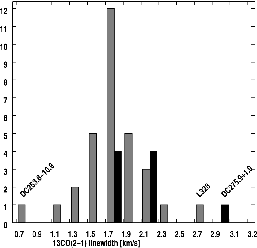
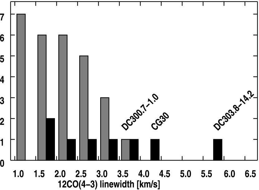
Figure 2: Histograms of the ¹³CO(2$\rightarrow$1) linewidth (left) and ¹²CO(4$\rightarrow$3) (right). Grey bars represent sources with no embedded stars, black bars represent sources with embedded IRAS sources.

In Figure 2, we show histograms of the linewidths of the two detected transitions. The distribution of the ¹³CO(2$\rightarrow$1) linewidth has a mean of 1.8 km s^-1 and a standard deviation of 0.4 km s^-1. The cores with embedded sources are represented by the black bars. It is noticeable that their distribution is generally skewed to higher values. The mean of their linewidths distribution is 2.0 km s^-1and the standard deviation is 0.4 km s^-1. Cores with embedded stars tend to be warmer and more turbulent, and their emission lines are therefore subject to more broadening, than are cores without embedded stars. If the gas kinetic temperature is typically 20 K, the corresponding optically thin thermal linewidth of CO is only 0.2 km s^-1, so the observed widths are due primarily to turbulent motions and optical depth effects. DC253.8-10.9 shows an exceptionally narrow line with only 0.8 km s^-1. It also is the weakest core in ¹³CO(2$\rightarrow$1). L328 has the broadest line of the cores with no embedded IRAS source at 2.7 km s^-1. This core has recently been found to have a VeLLO embedded (Lee, C.-W., in preparation). The widest line at 2.9 km s^-1 is emitted by DC275.9+1.9, which does have an embedded star (Bourke et al., 1995).

The distribution of the ¹²CO(4$\rightarrow$3) linewidth also shows that the lines from cores with embedded sources tend to be broader than lines from starless cores. The mean linewidth of cores with embedded stars is 3.2 km s^-1, with a standard deviation of 1.3 km s^-1. Cores with no embedded stars have a mean linewidth of 2.0 km s^-1, with a standard deviation of 0.7 km s^-1. For this histogram, we did not consider cores whose peak intensity is lower that 5$\sigma$. These omitted cores are DC302.6-15.9, L63, CB68, and L328. The widest line of all cores is found in DC303.8-14.2 at 5.8 km s^-1, which has an embedded star (Bourke et al., 1995). The widest line of cores with no embedded sources is emitted by DC300.7-1.0 with 3.5 km s^-1.

The survey of southern cores by Vilas-Boas et al. (1994) in ¹³CO(1$\rightarrow$ 0) reports an average linewidth of 0.8  km s^-1. The only source observed in both the Vilas-Boas et al. survey and this survey is CG30. Vilas-Boas et al. (1994) gives a linewidth of 1.19 km s^-1obtained with a resolution of 0.12 km s^-1. Using our high resolution spectrometer, we observed a linewidth of 1.2 $\pm$ 0.1 km s^-1, which is in good agreement with Vilas-Boas et al. (1994).

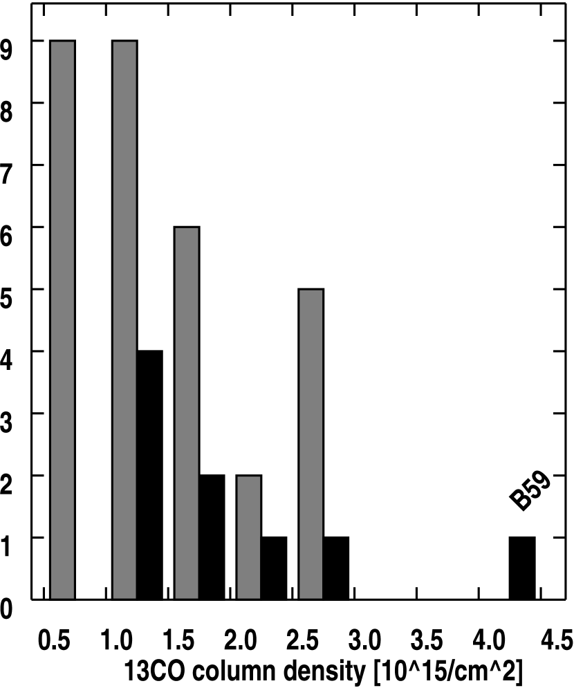
Figure 3: Histogram of the ¹³CO column density for all sources. Grey bars represent sources with no embedded stars, black bars represent sources with embedded IRAS sources.

A histogram of the ¹³CO column density is shown in Figure 3. The mean ¹³CO column density for cores with no embedded stars is 0.5 to 2.0 $\times$ 10¹⁵ cm^-2 and slightly higher, around 1.0 to 2.0 $\times$ 10¹⁵ cm^-2, for cores with embedded stars, which do not show ¹³CO column densities lower than 1.0 $\times$ 10¹⁵ cm^-2. Fifty-five percent of the cores have a ¹³CO column density between 0.5 to 1.5 $\times$ 10¹⁵ cm^-2, and 75% have column densities between 0.5 to 2.0 $\times$ 10¹⁵ cm^-2. Assuming a ¹³CO/H₂ ratio of 1.7 $\times$ 10^-6 (Wilson & Rood, 1994; Frerking et al., 1982), we can convert the ¹³CO column densities to the H₂ column density. The H₂ column density distribution has a mean of 1.9 $\times$ 10²¹ cm^-2 and a standard deviation of 0.7 $\times$ 10²¹ cm^-2 for cores with embedded sources. For all other sources the mean is 1.5 $\times$ 10²¹ cm^-2 and the standard deviation is 0.7 $\times$ 10²¹ cm^-2. Cores with embedded sources tend to have higher column densities. Seven of the observed cores lie in Ophiuchus which has a high level of star formation activity (Wilking, 1992). In these cores the H₂ column density assumes high values, with a mean of 3.7 $\times$ 10²¹ cm^-2 and a dispersion of 1.5 $\times$ 10²¹ cm^-2. Twenty-three cores lie within clouds where the star-forming activity is low (Vela, Musca, Coalsack, Chamaeleon II and III, Lupus, Scorpius). These cores have a mean H₂ column density of 2.7 $\times$ 10²¹ cm^-2 with a dispersion of 1.0 $\times$ 10²¹ cm^-2. This difference as an indicator of star-forming activity was also observed by Vilas-Boas et al. (2000) in a ¹³CO(1-0) survey of different (none of the sources in their and our survey overlap) dense condensations in dark clouds. Vilas-Boas et al. (2000) set the limit for star-formation-enabling H₂ column density to as high as 1.1 $\times$ 10²² cm^-2. This limit appears to be too high, considering our results for B59. B59 in Ophiuchus is the strongest core observed and has the exceptionally high ¹³CO column density of 4.3 $\times$ 10¹⁵ cm^-2 and H₂ column density of 7.3 $\times$ 10²¹ cm^-2, thus indicating strong star formation activity. A group of embedded sources has already been found in this core (Brooke et al., 2007).

3.1 Large Velocity Gradient Analysis

For a more detailed analysis of our data, we chose only the cores most suitable for the purpose: cores with strong ($>$ 5$\sigma$) emission in both ¹³CO(2$\rightarrow$1) and ¹²CO(4$\rightarrow$3). We also made sure there was no large pointing offset between intensity peaks at the two wavelengths. In Figures 4a to 4e, we present maps of the nine cores chosen for the LVG analysis. The AST/RO contour maps are superimposed on optical images from the Digital Sky Survey (DSS) retrieved from SkyView (McGlynn et al., 1996). The cores are shown in order of ascending R.A. We present the majority of cores superimposed on 15$\hbox{${}^{\prime}$}\times$ 15^′ images, but AST/RO map sizes vary. Maps in the same row show the same source, the left column shows the ¹³CO(2$\rightarrow$1) emission, the right column shows the ¹²CO(4$\rightarrow$3). All maps are labeled with the source name, the observed transition, and the maximum integrated intensity in K  km s^-1. Contours in all maps are in percentage of the peak intensities. We show contour levels in steps of 10% of the highest contour, whose value is given in each figure. The first maps on each page show the AST/RO effective beamsizes of 216^′′ at 220 GHz and 117^′′ at 461 GHz. Since the maps were made using Gaussian interpolation, the effective beamsizes in the maps are slightly larger than the actual telescope beamsizes.

Maps that are larger than 15$\hbox{${}^{\prime}$}\times$ 15^′ are shown in order of ascending R.A. after the set of 15$\hbox{${}^{\prime}$}\times$ 15^′ maps. The top figure shows the ¹³CO(2$\rightarrow$1) map, the bottom figure shows the ¹²CO(4$\rightarrow$3) map. In cases with more than one source per map, the sources are labeled individually.

We can estimate the kinetic temperature $T_{kin}$, and the number density of molecular hydrogen $n(H{{}_{2}})$, using a Large Velocity Gradient (LVG) analysis of the radiative transfer (Goldreich & Kwan, 1974). Our LVG radiative transfer code has been developed and applied by M. Yan and S. Kim (Kim et al., 2002) and has been implemented as a java applet . This model simulates a plane-parallel cloud geometry and uses the CO collisional rates from Turner (1995), newly-derived values for the H₂ ortho-to-para ratio ($\approx$ 2), and the collisional quenching rate of CO by H₂ impact (Balakrishnan et al., 2002). The model has two input parameters: the ratio of ¹²CO to ¹³CO abundance, and the ratio $X$(CO)/$\nabla V$, where $X$(CO) is the fractional CO abundance and $\nabla V$ denotes the velocity gradient. The abundance ratio ¹²CO/¹³CO is taken to be 60 in dense molecular clouds (Wilson & Rood, 1994). The ¹²CO/H₂ ratio is taken to be 10^-4 (Frerking et al., 1982) (leading to a ¹³CO to H₂ ratio of 1.7 $\times$ 10^-6) and the velocity gradient across the cores 1  km s^-1 pc^-1.

The ¹²CO(4$\rightarrow$3) data were convolved with a Gaussian kernel to the lower ¹³CO(2$\rightarrow$1) resolution. The resulting peak intensities are listed in Table 4.

Although we were unable to detect any significant ¹²CO(7$\rightarrow$6) emission, we can use these data to derive a significant upper limit for this emission for each source. We convolved the higher resolution ¹²CO(7$\rightarrow$6) data with a Gaussian kernel to the ¹³CO(2$\rightarrow$1) resolution and derived a 3$\sigma$ upper limit for the emission through this relation:

$$\rm{3\sigma=3\times\frac{rms\times\sqrt{N}\times channelwidth\times 0.94}{FWHM(4-3)}}$$ (3)

where ‘rms’ is the rms noise of the co-added spectrum. N is the number of channels over which the rms was measured (twice the expected linewidth of the ¹²CO(7$\rightarrow$6) line). ‘Channelwidth’ is the width of the acousto-optic spectrometer channels at this wavelength. FWHM(4-3) is the half-power width of the corresponding ¹²CO(4$\rightarrow$3) line. The factor of 0.94 comes from the relation for Gaussian profiles: FWHM $\times$ peak = 0.94 $\times$ area.

The results are shown in Table 4, where upper and lower limits are denoted u.l. and l.l. Since the line brightness temperature T${}^{12}_{7\rightarrow 6}$ of the ¹²CO(7$\rightarrow$6) line is an upper limit, the ratio $T^{12}_{7\rightarrow 6}$/$T^{12}_{4\rightarrow 3}$, the kinetic temperature and the H₂ density are also upper limits. To obtain the lower temperature and density limits, we assume no ¹²CO(7$\rightarrow$6) emission at all: T${}^{12}_{7\rightarrow 6}$ = 0.

As can be seen from Table 4, the lower temperature limits average to 16 K and are not greater than 20 K for any source. The distribution of the upper temperature limits have an average of 26 K. The H₂ density distribution is fairly uniform, ranging from 10^2.7 cm^-3 to 10^3.7 cm^-3 with an average lower limit of 10^2.9 cm^-3 and an average upper limit of 10^3.3 cm^-3 for all sources. Due to the small sample size, we cannot detect a significant difference in the mean densities of cores with and without embedded stars.

3.2 Masses

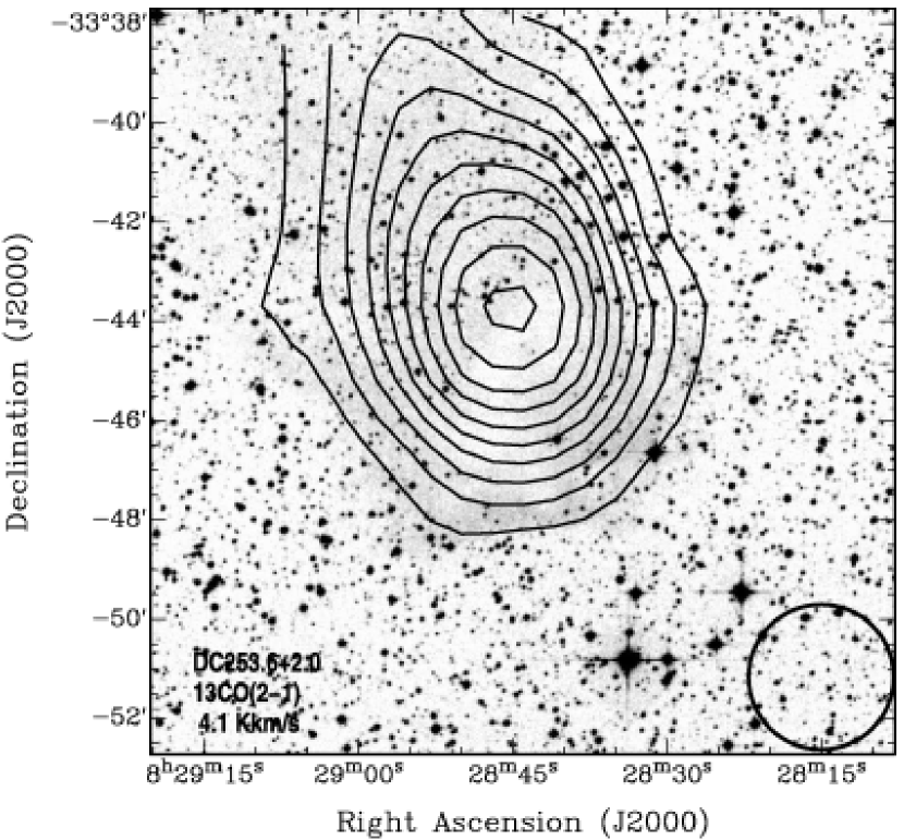
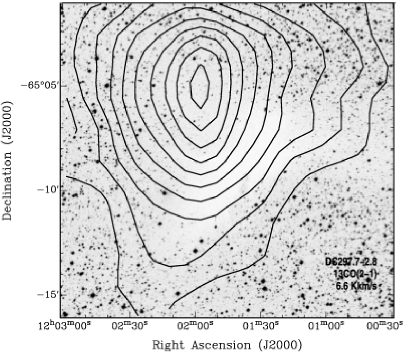
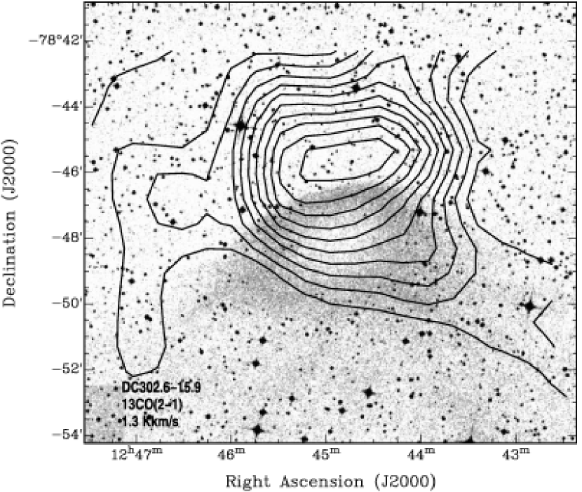
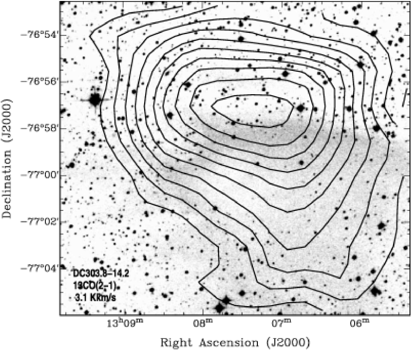
Figure 5: Maps of DC253.6+2.0, DC297.7-2.8, DC302.6-15.9, and DC303.8-14.2 in ¹³CO(2$\rightarrow$1). The effective beamsize of 216^′′ is indicated by the circle.

Nine cores were chosen for the derivation of their masses. We selected cores whose half-peak contours in ¹³CO(2$\rightarrow$1) are closed to derive the cores’ masses. These cores are also resolved. Maps of the selected sources are presented in Figures 4 and 5. We show contour levels in steps of 10% of the highest contour, whose value is given in each figure. DC302.6-15.9 and DC303.8-14.2 are at very high elevation (79^∘ and 77^∘) and possibly suffer from a systematic pointing offset as suggested from the background image. For the calculation of their masses, a potential pointing offset is irrelevant. There is no evidence that other cores show a similar pointing offset. We can obtain the total mass of the core using

$$M=\langle m\rangle\int_{A}N(H_{2})\ dA$$ (4)

where $A$ is the projected area and $\langle m\rangle$ is the mean mass per hydrogen molecule. This mean mass per hydrogen molecule $\langle m\rangle$ accounts for a helium abundance of one helium atom per five hydrogen molecules. We take into account that the sources are not spherical, but elliptical, and list their two radii (major and minor axes) in Table 5. We derive an average ¹³CO column density for the core area that is defined by the 50% peak intensity contour by co-adding all data that were taken in this area and making use of equation (1). This conversion assumes an excitation temperature of $T_{ex}$ = 10 K. Up to $T_{ex}$ = 40 K, the effect of this parameter on the ¹³CO column density is less than a factor of 2. By assuming a ratio of 1.7 $\times$ 10^-6 between ¹³CO and H₂ (Wilson & Rood, 1994; Frerking et al., 1982), we then convert the ¹³CO column densities to the H₂ column densities listed in Table 5 and use the relation above to determine their masses. Their distances are quoted from the literature: DC259.5-16.4, CG30, DC267.4-7.5, DC253.6+2.0, and DC274.2-0.4 lie within the Vela complex at 450 $\pm$ 50 pc (Woermann et al., 2001); DC297.7-2.8 is associated with the Coalsack at 150 $\pm$ 30 pc (Franco, 1995; Corradi et al., 1997); DC302.6-15.9 and DC303.8-14.2 lie in the Chamaeleon cloud complexes at distances between 150 - 180 pc (Whittet et al., 1997; Knude & Høg, 1998); L100 lies within Ophiuchus at 125 $\pm$ 25 pc (de Geus et al., 1989). The results are listed in Table 5. If the upper limit kinetic temperature was obtained through the LVG analysis, we list it again.

The derived masses range from 4 to 255 M_⊙, depending on the size of the core. The highest-mass core, DC267.4-7.5, is also the largest. The smallest and weakest core, DC302.6-15.9, does have the lowest mass. A correlation between temperature and mass cannot be established.

We have found three cores whose masses have been derived from different observations. Vilas-Boas et al. (1994) derived the mass of CG30 to be 43 M_⊙ with an uncertainty of a factor of 2.5, but they also quote a shorter distance of 300 pc. With a distance of 450 pc, this mass would be 97 M_⊙, which is within a factor of two of our value (58 M_⊙). Bourke et al. (1997) have calculated the mass of DC297.7-2.8 to be 40 M_⊙, using a larger radius and larger distance for the source. With the distance we use, 150 pc, this value becomes 23 M_⊙, which is also within a factor of two of our value (12 M_⊙). Keto & Myers (1986) calculated the mass of DC259.5-16.4 to be 41 M_⊙, but they used the much smaller distance of 100 pc. Combining their observations with a distance of 450 pc leads to a mass for DC259.5-16.4 of 830 M_⊙.

4 SUMMARY AND CONCLUSIONS

In order to study the physical conditions in small isolated molecular clouds, we have mapped 40 cores in the southern hemisphere in ¹³CO(2$\rightarrow$1), ¹²CO(4$\rightarrow$3), and ¹²CO(7$\rightarrow$6) with AST/RO. The sources cover all cores visible from the South Pole ($\delta\,<\,-16\hbox{${}^{\circ}$}$) from the initial c2d source list (Evans et al., 2003). The AST/RO survey at millimeter and submillimeter wavelengths provides a direct diagnostic of the dominant gas components in the clouds. By observing the ¹²CO and ¹³CO lines, we have obtained information about the physical conditions within the cloud. ¹³CO is a tracer of moderately dense ($\sim$ 10³ cm^-3) gas. It is generally optically thin and hence is a good tracer of column density. It probes the outer regions of dense cores (10 to 20 K), but not the densest interiors where a small percentage of the total ¹³CO mass is depleted within a small percentage of the total size ($\sim$ 10³ AU; Tafalla et al. (2002)). The most important submillimeter measurement is the ¹²CO(4$\rightarrow$3) transition: this line is the lowest-lying of the mid-J CO lines that constrain density rather strongly. These data have been used to determine meaningful conclusions about the physical properties of the molecular cores. The detection of the ¹²CO(7$\rightarrow$6) transition was unlikely, since the molecular cores are rather cold. From our data, we were able to put upper limits on the intensities in this transition, which were important for a Large Velocity Gradient (LVG) analysis.

We find typical ¹³CO(2$\rightarrow$1) linewidths to be 1.8 to 2.3 km s^-1 for cores with embedded stars and 1.6 to 1.9 km s^-1for all others. The slightly higher values for sources with embedded stars result from warmer gas whose emission is more subject to thermal and turbulent broadening of the lines. Only 10 out of 40 cores have linewidths outside the 1.5 to 2.1 km s^-1 window, the smallest being 0.8 km s^-1 and the largest being 2.7 km s^-1. The largest linewidth is found in DC275.9+1.9, a core with an embedded star; the smallest is found in the rather weak source DC253.8-10.9, with no signs of star formation.

The distribution of the ¹²CO(4$\rightarrow$3) linewidth is much broader. Typical values lie in the range of 1.6 to 2.3 km s^-1 for cores with no embedded sources, and 2.6 to 3.7 km s^-1 for cores with embedded stars. The distribution of their linewidths is rather flat, with the largest linewidth of 5.8 km s^-1 occurring in DC303.8-14.2. From the ¹³CO line intensities, we were able to derive the ¹³CO column density and the H₂ column density ($\S$ 3). The mean of the ¹³CO column density is found to be 1.9 $\times$ 10¹⁵ cm^-2 for cores with embedded stars, and 1.5 $\times$ 10¹⁵ cm^-2 for all others. Due to its exceptionally strong ¹³CO(2$\rightarrow$1) line intensity, B59 also stands out here with a ¹³CO column density of 4.3 $\times$ 10¹⁵ cm^-2 and an H₂ column density of 7.3 $\times$ 10²¹ cm^-2.

For nine cores, we determined the kinetic temperature and molecular hydrogen density through an LVG analysis. For the ¹²CO(7$\rightarrow$6) transition, we determined upper intensity limits, since we have no significant detection of this line. As a result, all temperatures and densities are also upper limits. In addition, we give a lower temperature limit, assuming the absence of ¹²CO(7$\rightarrow$6) emission. For these nine cores, four of which have embedded stars, we find an average lower temperature limit of 16 K and an average upper limit of 26 K. The lower temperature limit is smaller than 21 K for all cores. The average upper limit on the molecular hydrogen density was found to be 10^3.3 cm^-3 for all cores. The average lower limit on the molecular hydrogen density was found to be 10^2.9 cm^-3. Due to the small sample size, we cannot detect a significant difference between the mean densities of cores with and without embedded stars.

We have obtained masses for nine cores. They range from 4 to 255 M_⊙, depending on the size of the core. A correlation between temperature or density and mass cannot be established, which is mainly due to the small sample size.

In general, the sources in this survey behave rather uniformly with only very few exceptions. Cores with embedded sources tend to have larger linewidths and higher ¹³CO column density than cores with no embedded stars.

From the comparison to previously published CO surveys of molecular cores (Keto & Myers, 1986; Vilas-Boas et al., 1994, 2000), we can say that the c2d sample of molecular cores has a range of properties (linewidth, column density, size, mass, embedded stars) similar to those of past studies. Only three sources from the sample covered in this survey have previously been observed in other CO surveys, albeit in lower rotational transitions. To obtain even more accurate results with an LVG analysis, a survey of these sources at one other CO transition would be very valuable.

Table 1: Source list.

Source name	Other names	$\alpha$ [J2000]	$\delta$ [J2000]	13CO(J=2$\rightarrow$1)	12CO(J=4$\rightarrow$3)
		[ $\!\!{}^{\rm h}$  $\!\!{}^{\rm m}$  $\!\!{}^{\rm s}$]	[∘ ′ ′′]	$\alpha$[′]$\times\delta$[′]	$\alpha$[′]$\times\delta$[′]
DC259.5-16.4	BHR22	07 14 12.2	-48 29 10	9 $\times$ 9	9 $\times$ 9
DC253.8-10.9	BHR14	07 29 32.7	-41 10 30	9 $\times$ 9	9 $\times$ 9
DC255.4-3.9	BHR16	08 05 26.3	-39 08 56	9 $\times$ 9	9 $\times$ 9
$\star$ CG30, CG31A-C	BHR12, BHR9-11	08 09 04.0	-36 00 51	30 $\times$ 30	24.5 $\times$ 23
DC257.3-2.5	-	08 17 09.3	-39 52 25	9 $\times$ 15	9.5 $\times$ 15
DC266.0-7.5	-	08 21 22.9	-49 50 47	9 $\times$ 9	9 $\times$ 9
$\star$ DC267.4-7.5	BHR36	08 25 48.3	-51 01 18	12 $\times$ 15	11.5 $\times$ 12
DC267.5-7.4	BHR37	08 26 37.0	-51 02 31	9 $\times$ 9	9 $\times$ 9
DC253.6+2.9	BHR13	08 28 44.0	-33 45 12	15 $\times$ 15	14.5 $\times$ 15
DC267.6-6.4	BHR40	08 32 00.8	-50 32 51	15 $\times$ 15	9 $\times$ 9
DC269.4+3.0	BHR43	09 22 22.0	-45 50 25	12 $\times$ 9	12.5 $\times$ 9
DC274.2-0.4	BHR53	09 28 47.0	-51 36 40	9 $\times$ 9	7 $\times$ 7.5
DC272.5+2.0	BHR47	09 31 02.8	-48 38 22	9 $\times$ 9	11 $\times$ 6.5
$\star$ DC275.9+1.9	BHR55	09 46 46.0	-51 05 12	9 $\times$ 9	9.5 $\times$ 6.5
DC291.0-3.5	-	10 59 43.0	-63 43 43	15 $\times$ 15	15 $\times$ 15
DC291.1-1.7	BHR59	11 06 52.0	-62 06 43	9 $\times$ 9	9 $\times$ 9
$\star$ DC297.7-2.8	BHR71	12 01 35.9	-65 08 37	15 $\times$ 15	-
DC300.2-3.5	BHR75	12 24 19.0	-66 11 52	9 $\times$ 9	11.5 $\times$ 9
Mu8	Musca Dark Cloud	12 29 35.0	-71 09 35	15 $\times$ 21	15 $\times$ 21
DC300.7-1.0	BHR77	12 31 34.0	-63 44 32	15 $\times$ 15	15 $\times$ 15
DC301.2-0.4	BHR78	12 36 15.0	-63 11 39	15 $\times$ 15	9 $\times$ 9
DC302.6-15.9	BHR84	12 44 57.6	-78 48 21	15 $\times$ 12	15 $\times$ 9.5
$\star$ DC302.1+7.4	BHR83	12 45 38.5	-55 25 18	9 $\times$ 9	7.5 $\times$ 9
$\star$ DC303.8-14.2	BHR86	13 07 35.7	-77 00 05	15 $\times$ 15	12 $\times$ 15
DC327.2+1.8	BHR111	15 42 19.2	-52 48 09	9 $\times$ 9	9 $\times$ 9
DC339.1+11.7	BHR129	15 59 03.6	-37 36 57	15 $\times$ 12	15 $\times$ 12.5
DC338.6+9.5	BHR126	16 04 28.0	-39 37 56	9 $\times$ 9	9.5 $\times$ 7.5
DC337.6+7.6	-	16 08 21.0	-41 42 19	18 $\times$ 18	17.5 $\times$ 18
$\star$ L43	RNO91	16 34 36.2	-15 46 57	15 $\times$ 15	15 $\times$ 15
DC346.0+7.8	B231	16 36 54.7	-35 36 08	9 $\times$ 12	9.5 $\times$ 12
DC346.3+7.8	-	16 37 44.9	-35 27 53	9 $\times$ 9	9.5 $\times$ 7.5
DC346.4+7.9	BHR144	16 37 33.0	-35 14 11	9 $\times$ 9	9 $\times$ 9
L63	-	16 50 11.0	-18 04 34	15 $\times$ 15	15 $\times$ 12.5
$\star$ CB68	L146	16 57 20.5	-16 09 02	15 $\times$ 12	15 $\times$ 12
$\star$ B59	L1746	17 11 22.1	-27 24 28	21 $\times$ 18	20.5 $\times$ 18
$\star$ L100	B62	17 16 01.0	-20 57 21	15 $\times$ 15	14.5 $\times$ 12
L1772	B65	17 19 32.7	-26 44 40	15 $\times$ 15	15 $\times$ 15
B72	CB83	17 23 45.0	-23 41 28	18 $\times$ 12	17.5 $\times$ 12.5
L328	CB131	18 17 00.0	-18 01 54	9 $\times$ 9	8 $\times$ 7.5

Table 2: Observed and derived parameters of the ¹³CO(2$\rightarrow$1) lines.

Source	$\alpha$ [J2000]	$\delta$ [J2000]	$v_{LSR}$	$\Delta v$	$\int T_{\mathrm{MB}}(v)\,dv$	rms Noise	$N_{{}^{13}CO}$
	[ $\!\!{}^{\rm h}$  $\!\!{}^{\rm m}$  $\!\!{}^{\rm s}$]	[∘ ′ ′′]	[ km s-1]	[ km s-1]	[K  km s-1]	[K]	[1015 cm-2]
DC259.5-16.4	07 14 03.2	-48 27 40	4.6	1.5 $\pm$ 0.1	2.7 $\pm$ 0.2	0.1	1.1
DC253.8-10.9	07 29 32.7	-41 07 30	-0.6	0.8 $\pm$ 0.1	1.5 $\pm$ 0.2	0.2	0.6
DC255.4-3.9	08 05 26.3	-39 07 26	9.8	2.4 $\pm$ 0.1	2.2 $\pm$ 0.2	0.2	0.9
CG31A-C	08 08 41.8	-35 54 51	6.7	1.9 $\pm$ 0.1	6.0$\pm$ 0.2	0.2	2.4
$\star$ CG30	08 09 26.3	-36 02 21	6.5	1.2 $\pm$ 0.1	4.0 $\pm$ 0.2	0.1	1.6
DC257.3-2.5	08 17 17.1	-39 47 55	8.8	2.0 $\pm$ 0.2	6.8 $\pm$ 0.5	0.6	2.7
DC266.0-7.5	08 21 22.9	-49 47 47	4.4	1.7 $\pm$ 0.1	4.8 $\pm$ 0.2	0.1	1.9
$\star$ DC267.4-7.5	08 25 48.3	-50 59 48	5.8	1.7 $\pm$ 0.1	5.3 $\pm$ 0.2	0.2	2.1
DC267.5-7.4	08 26 46.5	-51 04 01	6.5	1.5 $\pm$ 0.1	2.8 $\pm$ 0.2	0.2	2.9
DC253.6+2.9	08 28 44.0	-33 43 42	7.3	1.7 $\pm$ 0.1	4.7 $\pm$ 0.2	0.2	1.9
DC267.6-6.4	08 32 10.2	-50 31 21	6.3	1.6 $\pm$ 0.1	2.8 $\pm$ 0.2	0.1	1.1
DC269.4+3.0	09 22 22.0	-45 54 55	-2.9	1.3 $\pm$ 0.2	1.9 $\pm$ 0.1	0.1	0.9
DC274.2-0.4	09 28 47.0	-51 35 10	6.4	2.2 $\pm$ 0.2	2.5 $\pm$ 0.2	0.2	1.0
DC272.5+2.0	09 31 02.8	-48 36 52	-3.9	1.6 $\pm$ 0.2	1.6 $\pm$0.2	0.1	0.6
$\star$ DC275.9+1.9	09 46 36.5	-51 00 42	-4.9	2.9 $\pm$ 0.2	3.4 $\pm$ 0.2	0.1	1.3
DC291.0-3.5	11 00 10.1	-63 40 43	-3.8	1.7 $\pm$ 0.1	2.9 $\pm$ 0.2	0.1	1.1
DC291.1-1.7	11 07 04.8	-62 03 43	-4.2	1.8 $\pm$ 0.1	3.2 $\pm$ 0.2	0.1	1.3
DC297.7-2.8	12 01 57.0	-65 05 19	-3.9	2.1 $\pm$ 0.1	7.4 $\pm$ 0.2	0.2	2.9
DC300.2-3.5	12 25 03.5	-66 08 52	-5.2	1.9 $\pm$ 0.2	2.3 $\pm$ 0.2	0.2	0.9
Mu8	12 30 30.5	-71 03 35	3.8	1.7 $\pm$ 0.1	4.4 $\pm$ 0.2	0.1	1.7
DC300.7-1.0	12 31 20.5	-63 41 32	-5.5	1.1 $\pm$ 0.2	2.0 $\pm$ 0.1	0.2	0.8
DC301.2-0.4	12 36 01.7	-63 08 39	-4.4	1.6 $\pm$ 0.1	1.8 $\pm$ 0.2	0.1	0.7
DC302.6-15.9	12 44 26.8	-78 45 21	4.1	1.8 $\pm$ 0.1	1.8 $\pm$ 0.2	0.1	0.7
$\star$ DC302.1+7.4	12 45 49.1	-55 22 18	-14.7	2.1 $\pm$ 0.2	2.6 $\pm$ 0.2	0.1	1.0
$\star$ DC303.8-14.2	13 07 35.7	-76 57 05	4.3	2.1 $\pm$ 0.1	3.6 $\pm$ 0.2	0.1	1.4
DC327.2+1.8	15 42 49.0	-52 49 39	-0.4	2.0 $\pm$ 0.2	2.3 $\pm$ 0.2	0.1	0.9
DC339.1+11.7	15 59 11.2	-37 36 57	5.7	1.7 $\pm$ 0.1	4.3 $\pm$ 0.2	0.1	1.7
DC338.6+9.5	16 04 43.6	-39 36 26	5.2	1.0 $\pm$ 0.1	3.1 $\pm$ 0.2	0.1	1.2
DC337.6+7.6	16 08 21.0	-41 40 49	5.4	1.7 $\pm$ 0.1	7.1 $\pm$ 0.1	0.2	2.8
$\star$ L43	16 34 23.7	-15 49 57	1.0	1.8 $\pm$ 0.1	6.6 $\pm$ 0.2	0.1	2.6
DC346.0+7.8	16 36 54.7	-35 37 38	4.1	2.2 $\pm$ 0.1	5.4 $\pm$ 0.2	0.2	2.1
DC346.3+7.8	16 37 37.5	-35 30 53	3.8	1.8 $\pm$ 0.1	4.7 $\pm$ 0.2	0.2	1.9
DC346.4+7.9	16 37 47.7	-35 14 11	4.1	1.7 $\pm$ 0.1	4.0 $\pm$ 0.2	0.2	1.6
L63	16 49 52.1	-18 03 04	6.3	2.0 $\pm$ 0.1	7.3 $\pm$ 0.1	0.2	2.9
$\star$ CB68	16 56 49.3	-16 04 32	5.1	1.7 $\pm$ 0.1	3.2 $\pm$ 0.1	0.2	1.3
$\star$ B59	17 11 26.6	-27 25 58	3.7	2.1 $\pm$ 0.1	10.9 $\pm$ 0.2	0.2	4.3
$\star$ L100	17 16 01.0	-20 57 21	2.1	2.2 $\pm$ 0.1	4.1 $\pm$ 0.3	0.1	1.6
L1772	17 19 32.7	-26 41 40	3.9	1.8 $\pm$ 0.1	3.5 $\pm$ 0.2	0.2	1.4
B72	17 23 38.5	-23 38 28	5.4	1.7 $\pm$ 0.1	3.4 $\pm$ 0.2	0.2	1.3
L328	18 16 53.7	-18 03 24	7.4	2.7 $\pm$ 0.2	2.8 $\pm$ 0.2	0.2	1.1

Table 3: Observed parameters of the ¹²CO(4$\rightarrow$3) lines.

Source	$\alpha$ [J2000]	$\delta$ [J2000]	$v_{LSR}$	$\Delta v$	$\int T_{\mathrm{MB}}(v)\,dv$	rms Noise
	[ $\!\!{}^{\rm h}$  $\!\!{}^{\rm m}$  $\!\!{}^{\rm s}$]	[∘ ′ ′′]	[ km s-1]	[ km s-1]	[K  km s-1]	[K]
DC259.5-16.4	07 14 06.2	-48 28 10	4.2	3.0 $\pm$ 0.4	3.9 $\pm$ 0.4	0.4
DC253.8-10.9	07 29 32.7	-41 10 00	-1.1	3.1 $\pm$ 0.3	4.1 $\pm$ 0.3	0.3
DC255.4-3.9	08 05 18.6	-39 11 26	9.7	2.1 $\pm$ 0.3	3.2 $\pm$ 0.3	0.4
CG31A-C	08 09 01.5	-35 59 21	6.7	2.2 $\pm$ 0.1	14.4 $\pm$ 0.5	0.3
$\star$ CG30	08 09 33.7	-36 04 51	6.5	4.2 $\pm$ 0.3	11.0 $\pm$ 0.3	0.6
DC257.3-2.5	08 17 11.9	-39 51 25	8.6	1.4 $\pm$ 0.1	5.9 $\pm$ 0.4	0.4
DC266.0-7.5	08 21 13.6	-49 54 47	3.8	2.0 $\pm$ 0.2	4.9$\pm$ 0.3	0.3
$\star$ DC267.4-7.5	08 25 45.1	-50 59 18	5.5	1.8 $\pm$ 0.1	10.9 $\pm$ 0.2	0.2
DC267.5-7.4	08 26 56.1	-51 04 31	6.0	2.7 $\pm$ 0.2	5.9 $\pm$ 0.3	0.3
DC253.6+2.9	08 28 58.4	-33 47 12	6.3	1.3 $\pm$ 0.1	6.4 $\pm$ 0.3	0.3
DC267.6-6.4	08 32 03.9	-50 32 21	5.8	1.6 $\pm$ 0.1	5.2 $\pm$ 0.3	0.3
DC269.4+3.0	09 22 16.3	-45 47 25	-1.4	2.0 $\pm$ 0.2	3.3 $\pm$ 0.2	0.3
DC274.2-0.4	09 28 50.2	-51 36 40	5.9	2.2 $\pm$ 0.2	2.6 $\pm$ 0.2	0.2
DC272.5+2.0	09 31 11.9	-48 37 52	-3.8	2.7 $\pm$ 0.9	1.5 $\pm$ 0.2	0.3
$\star$ DC275.9+1.9	09 46 30.1	-51 01 12	-5.7	2.6 $\pm$ 0.3	4.2 $\pm$ 0.4	0.4
DC291.0-3.5	10 59 02.4	-63 40 43	-4.8	1.0 $\pm$ 0.1	5.0 $\pm$ 0.4	0.6
DC291.1-1.7	11 06 13.6	-62 03 13	-4.3	1.2 $\pm$ 0.1	3.5 $\pm$ 0.2	0.3
DC300.2-3.5	12 24 19.0	-66 12 52	-5.7	1.1 $\pm$ 0.1	2.7 $\pm$ 0.2	0.2
Mu8	12 28 07.6	-71 19 05	3.25	2.5 $\pm$ 0.3	6.4 $\pm$ 0.5	0.7
DC300.7-1.0	12 31 29.5	-63 44 32	-4.9	3.5 $\pm$ 0.1	5.9 $\pm$ 0.1	1.3
DC301.2-0.4	12 36 19.4	-63 11 09	-4.7	2.6 $\pm$ 0.5	2.4 $\pm$ 0.3	0.3
DC302.6-15.9	12 45 38.7	-78 47 21	3.8	1.7 $\pm$ 0.1	2.2 $\pm$ 0.1	0.5
$\star$ DC302.1+7.4	12 45 38.5	-55 24 48	-14.7	2.2 $\pm$ 0.3	3.7 $\pm$ 0.4	0.4
$\star$ DC303.8-14.2	13 07 26.8	-77 01 35	3.4	5.8 $\pm$ 0.5	6.7 $\pm$ 0.3	0.2
DC327.2+1.8	15 42 32.4	-52 48 09	-0.8	3.2 $\pm$ 0.5	3.1 $\pm$ 0.3	0.3
DC339.1+11.7	15 59 31.4	-37 36 57	5.1	1.3 $\pm$ 0.1	6.6 $\pm$ 0.5	0.5
DC338.6+9.5	16 04 33.2	-39 38 56	4.4	1.0 $\pm$ 0.1	3.6 $\pm$ 0.3	0.3
DC337.6+7.6	16 07 46.2	-41 43 49	4.7	1.7 $\pm$ 0.1	9.5 $\pm$ 0.1	0.5
$\star$ L43	16 34 25.8	-15 48 27	0.4	3.0 $\pm$ 0.3	14.8 $\pm$ 1.0	1.0
DC346.0+7.8	16 36 57.2	-35 36 38	3.3	1.8 $\pm$ 0.2	6.8 $\pm$ 0.4	0.4
DC346.3+7.8	16 37 47.4	-35 28 53	3.4	1.8 $\pm$ 0.1	7.1 $\pm$ 0.3	0.3
DC346.4+7.9	16 37 57.5	-35 15 11	3.3	1.6 $\pm$ 0.1	4.8 $\pm$ 0.2	0.3
L63	16 50 04.7	-18 01 04	5.8	1.2 $\pm$ 0.1	6.7 $\pm$ 0.2	1.4
$\star$ CB68	16 57 03.8	-16 03 32	5.6	3.4 $\pm$ 0.4	7.5 $\pm$ 0.4	1.2
$\star$ B59	17 11 17.6	-27 26 28	4.0	3.6 $\pm$ 0.3	18.1 $\pm$ 0.7	0.9
$\star$ L100	17 16 16.0	-21 01 51	1.4	1.8 $\pm$ 0.3	14.2 $\pm$ 1.6	0.4
L1772	17 19 50.6	-26 44 40	3.5	2.1 $\pm$ 0.2	5.1 $\pm$ 0.3	0.4
B72	17 23 04.7	-23 42 28	5.1	1.9 $\pm$ 0.3	6.0 $\pm$ 0.5	0.8
L328	18 17 02.1	-18 04 24	6.9	1.2 $\pm$ 0.3	3.3 $\pm$ 0.7	0.9

Table 4: Results from the LVG model.

Source	$\alpha$ [J2000]	$\delta$ [J2000]	T${}^{13}_{2\rightarrow 1}$	T${}^{12}_{4\rightarrow 3}$	T${}^{12}_{7\rightarrow 6}$	$\frac{T^{12}_{7\rightarrow 6}}{T^{12}_{4\rightarrow 3}}$	$\frac{T^{12}_{4\rightarrow 3}}{T^{13}_{2\rightarrow 1}}$	Tkin	Tkin	log n(H2)	log n(H2)
	[ $\!\!{}^{\rm h}$  $\!\!{}^{\rm m}$  $\!\!{}^{\rm s}$]	[∘ ′ ′′]	[K]	[K]	[K]			[K]	[K]	[cm-3]	[cm-3]
					u.l.	u.l.		u.l.	l.l.	u.l.	l.l.
DC259.5-16.4	07 14 03.2	-48 27 40	1.6	0.8	0.5	0.6	0.5	22	14	3.2	2.9
CG31A-C	08 08 49.2	-35 57 51	3.1	4.3	1.4	0.3	1.4	28	17	3.2	2.8
$\star$ CG30	08 09 26.3	-36 03 51	1.6	1.8	0.8	0.4	1.2	30	18	3.3	2.9
$\star$ DC267.4-7.5	08 25 48.3	-50 59 48	2.5	2.8	0.3	0.1	1.1	22	14	3.2	2.9
DC267.5-7.4	08 26 46.5	-51 04 01	1.6	1.5	0.4	0.3	0.9	26	15	3.2	2.9
DC274.2-0.4	09 28 47.0	-51 35 10	1.0	0.6	0.2	0.4	0.6	18	12	3.7	3.0
DC339.1+11.7	15 59 11.2	-37 36 57	2.3	3.4	1.3	0.4	1.5	34	19	3.1	2.8
$\star$ B59	17 11 19.8	-27 25 58	4.0	4.1	1.9	0.5	1.0	28	16	3.3	2.9
$\star$ L100	17 16 07.4	-20 57 21	1.7	2.3	0.6	0.3	1.4	30	20	3.1	2.7

Table 5: Masses derived from the H₂ column densities.

Source	Distance	Radius1	Radius2	N(H2)	Mass	Tkin
	[pc]	[pc]	[pc]	[1021 cm-2]	[M⊙]	u.l. [K]
DC259.5-16.4	450 $\pm$ 50	0.9	0.7	1.3	48 $\pm$ 12	22
$\star$ CG30	450 $\pm$ 50	0.8	0.7	1.8	58 $\pm$ 14	30
$\star$ DC267.4-7.5	450 $\pm$ 50	1.4	1.2	2.9	255 $\pm$ 60	22
DC253.6+2.0	450 $\pm$ 50	0.9	0.7	2.4	103 $\pm$ 26	$\cdots$
DC274.2-0.4	450 $\pm$ 50	0.8	0.7	1.5	56 $\pm$ 14	18
DC297.7-2.8	150 $\pm$ 30	0.2	0.3	3.3	12 $\pm$ 4	$\cdots$
DC302.6-15.9	150 $\pm$ 30	0.2	0.3	0.9	4 $\pm$ 2	$\cdots$
$\star$ DC303.8-14.2	178 $\pm$ 18	0.5	0.4	1.5	19 $\pm$ 4	$\cdots$
$\star$ L100	125 $\pm$ 25	0.4	0.4	1.9	14 $\pm$ 6	30

Figure 1a: ¹³CO(2$\rightarrow$1) (left) and ¹²CO(4$\rightarrow$3) (right) spectra with the highest integrated intensities. Coordinates of the spectra are given in Tables 2 and 3.

Fig. 1b. —

Fig. 1c. —

Fig. 1d. —

Fig. 1e. —

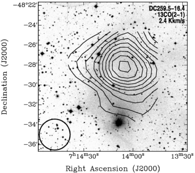
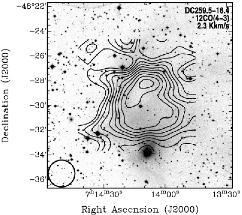
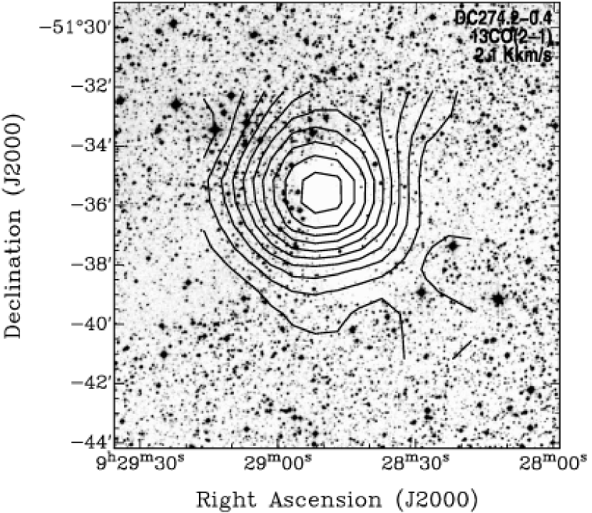
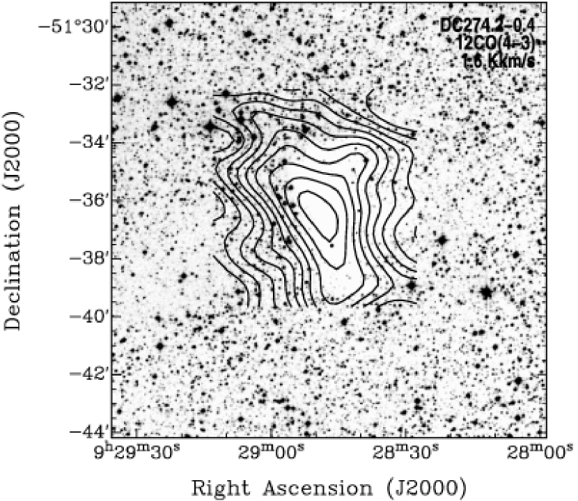
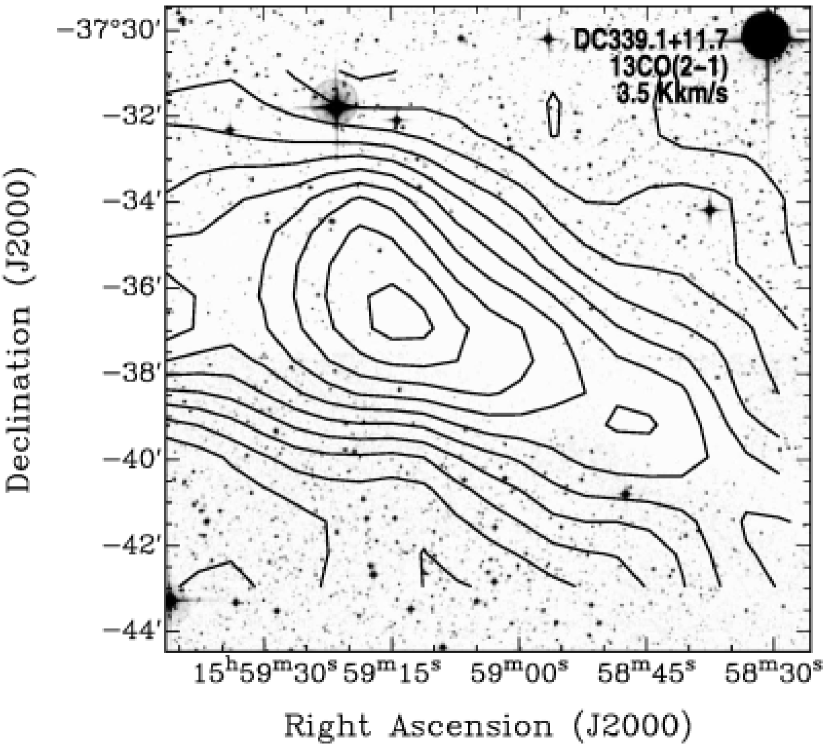
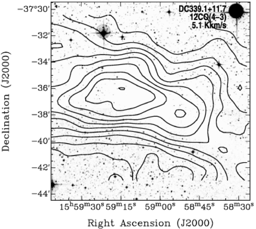
Figure 4a: Maps in 2 transitions of sources chosen for LVG analysis: ¹³CO(2$\rightarrow$1) (left/top) and ¹²CO(4$\rightarrow$3) (right/bottom). Contours are in steps of 10% of the peak intensity, listed in each map. The effective beamsizes are indicated by the circles and are 216^′′ in ¹³CO(2$\rightarrow$1) and 117^′′ in ¹²CO(4$\rightarrow$3). (a) DC259.5-16.4, DC274.2-0.4, DC339.1+11.7, (b) L100, (c) CG31A-C, CG30, (d) DC267.5-7.4, DC267.4-7.5, (e) B59

Fig. 4c. —

Fig. 4d. —

Fig. 4e. —

References

- Balakrishnan et al. (2002) Balakrishnan, N., Yan, M., & Dalgarno, A. 2002, ApJ, 568, 443
- Bourke et al. (2005) Bourke, T. L., Crapsi, A., Myers, P. C., Evans, N. J., Wilner, D. J., Huard, T. L., Jørgensen, J. K., & Young, C. H. 2005, ApJ, 633, L129
- Bourke et al. (1995) Bourke, T. L., Hyland, A. R., & Robinson, G. 1995, MNRAS, 276, 1052
- Bourke et al. (1997) Bourke, T. L., et al. 1997, ApJ, 467, 781
- Bourke et al. (2006) Bourke, T. L., et al. 2006, ApJ, 649, L37
- Brooke et al. (2007) Brooke, T. Y. et al., 2007, ApJ, 655, 364
- Chamberlin et al. (1997) Chamberlin, R. A., Lane, A. P., & Stark, A. A. 1997, ApJ, 476, 428
- Corradi et al. (1997) Corradi, W. J. B., Franco, G. A. P., & Knude, J. 1997, A&A, 216, 44
- Dunham et al. (2006) Dunham, M. M., et al. 2006, ApJ, 651, 945
- Evans et al. (2003) Evans, N. J., et al. 2003, PASP, 115, 965
- di Francesco et al. (2006) Di Francesco, J., Evans, N. J., Caselli, P., Muers, P., C., Shirley, Y., Aikawa, Y., & Tafalla, M. 2006, Protostars and Planets V review, (astro-ph/0602379)
- Franco (1995) Franco, G. A. P. 1995, A&AS, 114, 105
- Frerking et al. (1982) Frerking, M. A., Langer, D. W., & Wilson, R. W. 1982, ApJ, 262, 590
- de Geus et al. (1989) de Geus, E. J., de Zeeuw, P. T., & Lub, J. 1989, A&A, 216, 44
- Goldreich & Kwan (1974) Goldreich, P., & Kwan, J. 1974, ApJ, 189, 441
- Honingh et al. (1997) Honingh, C. E., Haas, S., Hottgenroth, D., Jacobs, K., & Stutzki, J. 1997, in 8th Int. Symp. on Space Terahertz Technology, eds. R. Blundell & E. Tong (Cambridge: Harvard Univ.), 92
- Huard et al. (2006) Huard, T. L., et al. 2006, ApJ, 640, 391
- Keto & Myers (1986) Keto, E. R., & Myers, P. C. 1986, ApJ, 304, 466
- Kim et al. (2002) Kim, S., Martin, C. L., Stark, A. A., & Lane, A. P. 2002, ApJ, 580, 896
- Knude & Høg (1998) Knude, J., & Høg 1998, A&A, 338, 897
- Kooi et al. (1992) Kooi, J. W., Man, C., Phillips, T. G., Bumble, B., & LeDuc, H. G. 1992, IEEE Trans. Microwave Theory and Techniques, 40, 812
- Lane (1998) Lane, A. P. 1998, in ASP Conf. Ser. 141, Astrophysics From Antarctica, eds. G. Novack & R. H. Landsberg (San Francisco: ASP), 289
- Lee & Myers (1999) Lee, C. W., & Myers, P. C. 1999, ApJS, 123, 233
- McGlynn et al. (1996) McGlynn, T., Scollick, K., & White, N. 1996, SkyView: The Multi-Wavelength Sky on the Internet, McLean, B.J. et al., New Horizons from Multi-Wavelength Sky Surveys, Kluwer Academic Publishers, IAU Symposium No. 179, p465.
- Myers et al. (1987) Myers, P. C., Fuller, G. A., Mathieu, R. D., Beichman, C. A., Benson, P. J., Schild, R. E., & Emerson, J. P. 1987, ApJ, 319, 340
- Myers et al. (1983) Myers, P. C., Linke, R. A., & Benson, P. J. 1983, ApJ, 264, 517
- Nielsen et al. (1998) Nielsen, A. S., Olberg, M., Knude, J., & Booth, R. S. 1998, A&A, 336, 329
- Oberst et al. (2006) Oberst, T. E., et al. 2006, ApJ, 652, L1250
- Otrupcek et al. (2000) Otrupcek, R. E., Hartley, M., & Wang, J.-S. 2000, Publ. Ast. Soc. of Australia, 17, 92
- Schieder et al. (1989) Schieder, R., Tolls, V., & Winnewisser, G. 1989, Exp. Astron., 1, 101
- Stark et al. (2001) Stark, A. A., et al. 2001, PASP, 113, 567
- Tafalla et al. (2002) Tafalla, M., Myers, P. C., Caselli, P., Walmsley, C. M., & Comito, C. 2002, ApJ, 569
- Turner (1995) Turner, B. E. 1995, ApJ, 455, 556
- Vilas-Boas et al. (1994) Vilas-Boas, J. W. S., Myers, P. C., & Fuller, G. A. 1994, ApJ, 433, 96
- Vilas-Boas et al. (2000) Vilas-Boas, J. W. S., Myers, P. C., & Fuller, G. A. 2000, ApJ, 532, 1038
- Walker et al. (1992) Walker, C. K., Kooi, J. W., Chan, M., Leduc, H. G., Schaffer, P. L., Carlstrom, J. E., & Phillips, T. G. 1992, Int. J. Infrared MM Waves, 13, 785
- Ward-Thompson et al. (2006) Ward-Thompson, D., Andr, P., Crutcher, R., Johnstone, D., Onishi, T., & Wilson, C. 2006, Protostars and Planets V review, (astro-ph/0603475)
- Wilking (1992) Wilking, B. A. 1992, in Low Mass Star Formation in Southern Molecular Clouds, ESO Scientific Report No. 11, ed. B. Reipurth, (ESO: Garching), p.159
- Whittet et al. (1997) Whittet, D. C. B., Prusti, T., Franco, G. A. P. Gerakines, P. A., Kilkenny, D., Larson, K. A. & Wesselius, P. R. 1997, A&A, 327, 1194
- Wilson & Rood (1994) Wilson, T. L., & Rood, R. T. 1994, ARA&A, 191
- Woermann et al. (2001) Woermann, B., Gaylard, M. J., & Otrupcek, R. 2001, MNRAS, 325, 1213
- Young et al. (2004) Young, C. H., et al. 2004, ApJS, 154, 396