The COSMOS Survey: Hubble Space Telescope / Advanced Camera for Surveys (HST/ACS) Observations and Data Processing

Abstract

We describe the details of the Hubble Space Telescope (HST) Advanced Camera for Surveys / Wide Field Channel (ACS/WFC) observations of the COSMOS field, including the data calibration and processing procedures. We obtained a total of 583 orbits of HST ACS/WFC imaging in the F814W filter, covering a field that is 1.64 degrees² in area, the largest contiguous field ever imaged with HST. The median exposure depth across the field is 2028 seconds (one HST orbit), achieving a limiting point-source depth AB(F814W) = 27.2 (5 sigma). We also present details about the astrometric image registration, distortion removal and image combination using MultiDrizzle, as well as motivating the choice of our final pixel scale (30 milliarcseconds per pixel), based on the requirements for weak lensing science. The final set of images are publicly available through the archive sites at IPAC and STScI, along with further documentation on how they were produced.

1 Introduction

The Cosmic Evolution Survey (COSMOS: Scoville et al. 2007a) is the largest contiguous survey ever undertaken with the Hubble Space Telescope (HST), imaging a $\sim 2$ degree² equatorial field with the primary goal of addressing the coupled evolution of large-scale structure, star formation and galaxy activity. A key requirement for this type of cosmological survey is sensitive imaging at the highest possible angular resolution, particularly for all sources above $z\sim 0.5-1$ where $\lesssim 0\farcs 1$ angular resolution becomes crucial to resolving structure on sub-kpc scales. This approach was pioneered in the Hubble Deep Fields North and South (HDF: Williams et al. 1996, 2000) which achieved this level of angular resolution, albeit over a relatively small 5 arcminute² field. Subsequent surveys included the Hubble Ultra Deep Field (UDF: Beckwith et al. 2006) which went deeper over a somewhat larger 11 arcminute² area; the Great Observatories Origins Deep Survey (GOODS: Giavalisco et al. 2004) which was shallower but covered a larger 360 arcminute² area; and two larger and shallower surveys, each covering $\sim 700$ arcmin² (GEMS: Rix et al. 2004; AEGIS: Davis et al. 2006). COSMOS provides an additional factor $\sim 10$ increased coverage in area, and uses broader filters to reach deeper sensitivities which are crucial for obtaining the accurate galaxy morphology measurements required to construct mass maps based on weak lensing.

In addition to the HST data, the COSMOS survey also contains a wealth of ancillary data obtained at other ground-based and space-based telescopes, including X-ray, infrared, sub-mm and radio imaging, as well as comprehensive spectroscopic programs, which are all summarized in Scoville et al. (2007a). The present paper describes the details of the HST observations and data processing that we used to construct the imaging datasets which form the foundation for the majority of the work in the COSMOS survey; see also Scoville et al. (2007b) for an overview.

2 ACS Observations

2.1 ACS Tiling Strategy for the Full COSMOS Mosaic

The COSMOS survey was awarded a total of 590 orbits of HST observations to cover a large, contiguous field of “tiles” centered at 10:00:28.6, +02:12:21.0 (J2000) using the Advanced Camera for Surveys (ACS) Wide-Field Channel (WFC) detector, together with the F814W (“Broad I”) filter. The ACS/WFC is a mosaic detector consisting of two 2048x4096-pixel CCDs with 15$\,\mu$m pixels, corresponding to a spatial scale of $\sim 0\farcs 05$/pixel and a field of view of $\sim 202\arcsec\times 202\arcsec$. The detectors have a read noise of 5 e^-/pixel and a dark current rate of 0.0038 e^-/s/pixel; the observations were all obtained with a gain of 1, corresponding to a full-well depth of 84,700 electrons (thus above the maximum A-to-D conversion limit of 65,535 counts per pixel). The camera is mounted $\sim 6\arcmin$ off-axis from the principal optical axis of HST and is also tilted with respect to the focal plane of HST, resulting in a significant amount of skew distortion across the field, $\sim 7-10\%$ of the detector size. Hence the pixels are projected as skew trapezoids on the sky, with their shapes changing across the detector, and this distortion is removed during post-observation processing described further down.

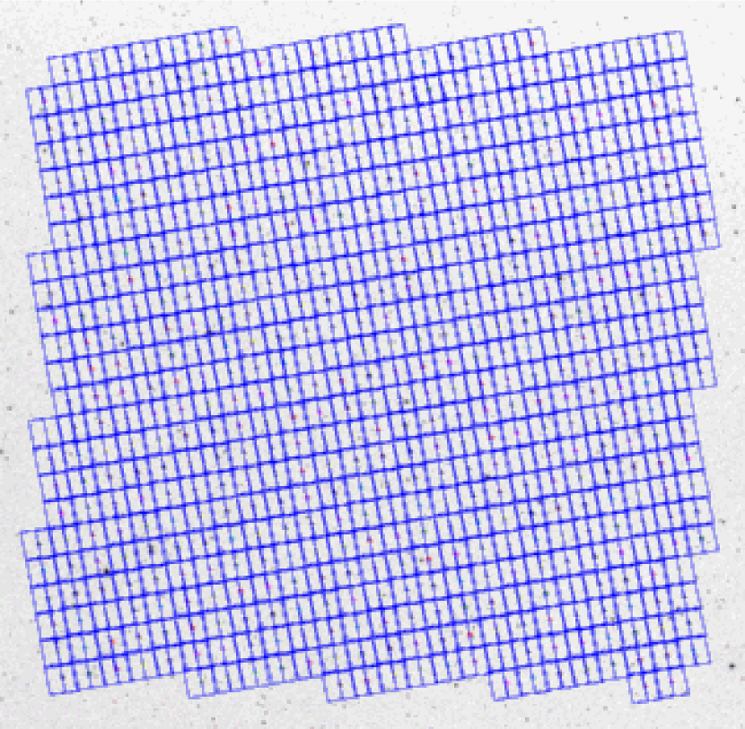
Figure 1: The final layout of the full mosaic of all the ACS/WFC F814W pointings, covering a total area of 1.64 degrees², or about $77\arcmin$ on a side. The field is centered at 10:00:28.6, +02:12:21.0 (J2000); the rectangle fully enclosing all the ACS imaging has lower left and upper right corners (RA,DEC J2000) at (150.7988^∘,1.5676^∘) and (149.4305^∘, 2.8937^∘).

Due to HST scheduling constraints, the observing program had to be divided between two HST observing cycles from May 2003 to June 2005, with 270 orbits allocated during Cycle 12 (HST Program ID 9822) and 320 orbits allocated during Cycle 13 (HST Program ID 10092). In order to maximize the amount of contiguous area coverage, it was required that all the tiles be obtained at the same orientation, thereby minimizing the amount of overlap between tiles to less than a few percent. Combining this with additional constraints on the orientation of HST with respect to the sun led to all the tiles being tilted about 10 degrees from North. In order to maintain the edges of the full field oriented approximately north-south and east-west (to maximize overlap with ancillary observations from other observatories) this led to slightly staggered edges, as shown in Figure 1. There are typically up to 16 orbits available per day on HST; since the allowable roll angles of HST change throughout the year, this meant that not all the tiles could be obtained at the same orientation, but that some of them had to be obtained at orientations that were rotated at 180^∘ relative to the default orientation. In addition, approval was granted to use 9 of the 590 orbits to obtain F475W observations (SDSS $g$) of a $3\times 3$ grid at the field center, as a pilot program to provide a demonstration of the value that two-filter HST ACS/WFC imaging would have for the main scientific goals of the project. Finally, two of the tile pointings failed due to problems with guide stars and were repeated, while two more tiles had severe problems with scattered light from adjacent stars and had to be repeated using slightly different pointings, offset from the original pointing by half a field in both directions (for which we used other orbits from the original total allocation). Thus the final contiguous area is 1.64 degrees², or approximately 77$\arcmin$ along each side, and contains data from a total of 583 orbits of HST ACS/WFC F814W imaging (including 2 additional orbits for repeat observations), with an additional 9 orbits of F475W imaging at the field center.

2.2 Cosmic Ray Splitting and Dither Strategy for each Tile

The total ACS/WFC exposure time obtained in F814W for each tile was 2028 seconds. Since cosmic rays impact between $\sim 2-6\%$ of the pixels on the ACS detectors during this length of exposure time, the observations for each tile were split into four equal-length exposures, each 507 seconds in duration, ensuring that $<1$ pixel out of 4096² would be impacted by cosmic rays in all four exposures according to statistical binomial probability. The exposure time of 507 seconds was the maximum that could be achieved within the nominal orbital duration of HST, after accounting for overheads due to readout, telescope motion and guidestar acquisition.

The four 507 second exposures for each tile were obtained using a “dither” pattern designed to improve the sampling of the point spread function (PSF), as well as covering the $\sim$3$\arcsec$ gap that is present between the two CCDs of the ACS/WFC. In the F814W filter, the intrinsic width of the PSF that is produced by the HST optics is $\sim 0\farcs 085$. However, this is significantly undersampled by the $0\farcs 05$ pixels of the ACS/WFC detector, and the final measured PSF in the combined images tends to be closer to $\sim 0\farcs 1$ as a result of convolution by the detector pixels as well as the pixel size of the final image. The undersampling can be mitigated to some extent by offsetting the detector in a dither pattern that provides subsampling of the PSF in different parts of each pixel during each exposure. As a consequence of the changing pixel size produced by the strong distortion of the ACS/WFC detectors, a given dither offset in arcseconds actually corresponds to different offsets in terms of pixels, and these offsets gradually vary across the detector, thereby further modulating the subsampling pattern achieved with four exposures.

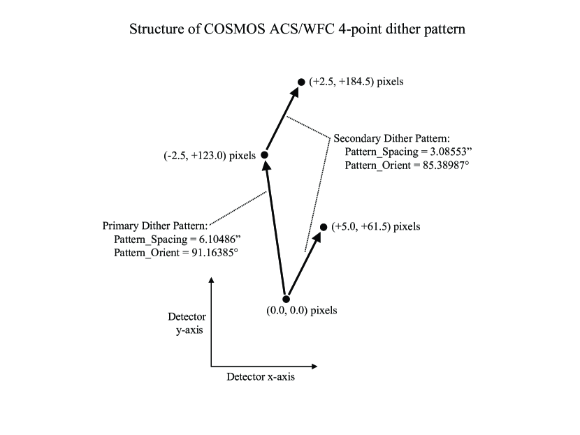
Figure 2: Schematic diagram of the dither pattern that we used for each set of four exposures that were obtained for each tile. By combining a 2-point primary dither pattern with a 2-point secondary pattern at each of the two primary dither points, along a slightly different orientation, each of the four pointings was thereby separated in increments of $\sim$3$\arcsec$ along the y-axis of the detector and increments of $\sim 0\farcs 25$ along the x-axis of the detector. The Pattern_Spacing and Pattern_Orient parameters shown are those that were used in the phase II file to construct these offsets. This pattern provided a combination of integer-pixel and half-pixel offsets, thereby ensuring that all four pointings would yield good sampling of any point on the sky by all four quadrants of a detector pixel. The distorted geometry of the detector provides an additional modulation of the phase of this half-pixel subsampling across the image, once all four exposures are combined.

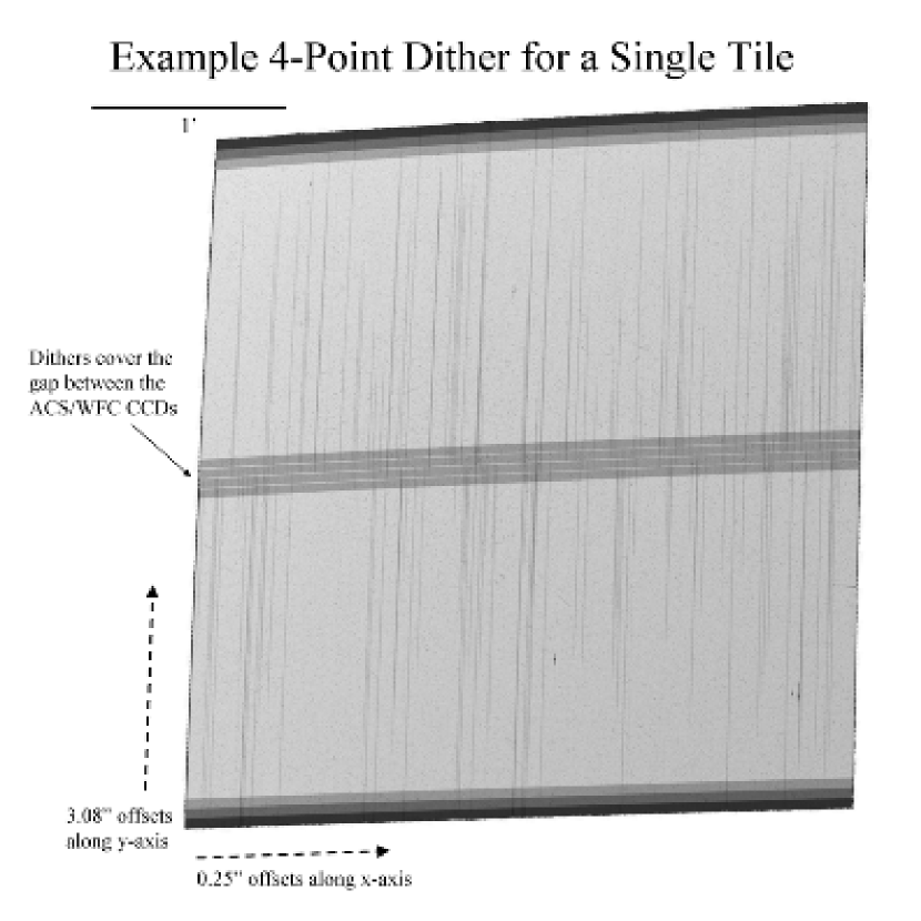
Figure 3: Example of a “weight” image corresponding to the combination of four ACS/WFC exposures of a single pointing, after initial processing through the pipeline. The image is equivalent to effective exposure time, with lighter regions indicating a longer combined exposure time on the final output pixels. Vertical dark lines correspond to bad columns, while the horizontal bands across the centre of the image correspond to the $\sim$3$\arcsec$ gap between the two detectors. This image demonstrates that the dither pattern successfully provided coverage of the gap by at least three exposures, as well as moving bad columns along the x-direction sufficiently to ensure that they were always covered by good pixels in the other exposures.

We chose a dither pattern designed to produce optimal subsampling of the PSF by ensuring that any given point would always be sampled by a different part of each detector pixel in the four exposures. This is achieved by offsetting the telescope in integer-pixel and half-pixel increments along both the x and y axes of the detector, thus the combination of four such offsets ensures that any given point on the sky is sampled by all four quadrants of a pixel during the four exposures. In addition, we added a $\sim$3$\arcsec$ offset along the y-direction of the dither pattern in order to cover the gap between the chips, as well as an offset of a few pixels along the x-direction of the dither pattern in order to ensure that bad columns and other defects were moved to a different part of the sky during each of the four exposures. The resulting dither pattern is shown in Figure 2, demonstrating how we implemented this using a combination of a primary 2-point dither pattern with an offset of $\sim$6$\arcsec$, together with a secondary 2-point dither pattern at each of the primary dither pattern points, providing an offset of $\sim$3$\arcsec$ along a slightly different orientation. The dither offset spacings and orientations in the two patterns provided the required pattern of half-pixel steps that was needed to ensure good subsampling to the level of $\sim$0.5 pixel across the entire detector. In Figure 3 we show the effective exposure time obtained after combining all four exposures for an example tile pointing, demonstrating the relatively uniform coverage across the detectors. Specifically, bad columns are moved around along the x-axis of the detectors, thereby ensuring that these points on the sky are covered by good pixels in three other exposures, and in addition the gap between the chips is always successfully covered by at least three exposures.

2.3 ACS Filter Selection

The primary scientific goal of the COSMOS HST ACS/WFC observations is to obtain the best possible rest-frame optical morphological information on $z\gtrsim 1$ galaxies, thereby necessitating observations at red wavelengths. We chose the broadest available filter on ACS in this wavelength range, namely the F814W (“Broad I”) filter. This filter is characterized by having a combination of exceptionally high transmission ($>90-95\%$) across an extremely wide wavelength range ($\sim\,$7300Å$\,-\,$9500Å); coupled with the red-sensitive ACS/WFC CCDs this provided optimal sensitivity to faint rest-frame visible morphological information at the redshifts of interest ($z\gtrsim 1$).

More specifically, the use of the F814W filter provides an additional $\sim 0.5\,$magnitude of depth relative to the narrower F775W (SDSS $i$) filter, for a given exposure time. This is important when comparing the depth of COSMOS to other surveys such as GEMS (Rix et al., 2004), GOODS (Giavalisco et al., 2004) or the UDF (Beckwith et al., 2006), all of which used the SDSS filter set, in particular F775W (SDSS $i$) and F850LP (SDSS $z$) at the red end of the spectrum, to provide sharp color discrimination through the use of certain spectral break features. This comes at the cost of a shallower depth per unit exposure time compared with the F814W filter, even though these other fields might be observable for a larger fraction of time with HST, since the total system throughput with the F814W filter is approximately equal to the sum of the F775W and F850LP filters. For this reason we chose the F814W filter for the COSMOS survey, to ensure the deepest possible morphological coverage with HST, while photometry using the SDSS filter set was obtained from ancillary ground-based observations using Subaru (Taniguchi et al., 2007).

For the pilot observations of the central $3\times 3$ tiles using a bluer filter, we chose the F475W (SDSS $g$) filter, motivated by the need to separate extinction-related effects from shape changes introduced by weak lensing. The F475W filter provides optimal throughput in the rest-frame near-UV for our target galaxies at $z\gtrsim 1$, for which weak lensing studies are the primary goal of the survey.

3 Data Reduction and Processing

We processed all the ACS data at STScI on a special-purpose computing cluster purchased especially for the project, consisting of 6 linux CPU nodes running pipeline scripts in parallel. As each observation was obtained, the individual exposures were delivered to the computing cluster where they were run through an IRAF/STSDAS pipeline that performed calibration, astrometric registration and cosmic ray cleaning, as well as final mosaic combination using MultiDrizzle (Koekemoer et al., 2002), which makes use of the Drizzle software (Fruchter & Hook, 2002) to remove the geometric distortion and map the input exposures onto a rectified output frame. Here we describe the details of each of these steps.

3.1 Initial Data Calibration

Each of the individual 507 second exposures was first run through the basic steps of ACS calibration using the IRAF/STSDAS task calacs, which performs bias and dark subtraction, gain correction, flat fielding, and identification of bad pixels. Each dataset was retrieved and run through this pipeline as soon as possible after the observation in order to make the data available quickly; this generally necessitated a second-pass calibration a few weeks later with more accurate reference files, in particular using dark and bias reference files that could be created using dark and bias exposures obtained contemporaneously with the data.

After basic calibration, several additional effects also had to be corrected in the data. In many cases, low-level residual background was present in the images, typically due to scattered light, and this was removed by constructing a master scattered-light image for the entire dataset through medianing, and then scaling and subtracting this from each individual exposure. In addition, the ACS/WFC CCDs are read out by four amplifiers (two for each CCD), and their bias levels often vary by a few tenths of a count which is not accounted for in the overscan bias calibration, therefore this was measured and corrected for each exposure.

Finally, the charge transfer efficiency (CTE) of the detectors is gradually deteriorating over time, as a result of charge traps in the pixels created by cosmic ray hits. This results in lost flux as the charge from each pixel is transferred down the CCD columns during readout, as well as producing trails as the traps release their charge after it has passed through. This effect is most severe for pixels that are furthest from the amplifiers, and for faint sources with minimal sky background. Its severity is reduced for sources on higher backgrounds (since there are a finite number of traps in a given pixel, thereby losing a progressively smaller fraction of the flux for brighter pixels). Ideally this effect would be corrected for on a pixel-by-pixel basis in the raw images but this requires a complete physical understanding of the effect, which is still under development. However, the effect can be quantified sufficiently well that it can be used to apply a post-processing correction to measured morphological and photometric properties of sources in the images, particularly relevant to the COSMOS weak lensing studies (Rhodes et al., 2007), based on a knowledge of the source positions and fluxes, together with the sky background values for the exposures involved.

3.2 Astrometric Image Registration

After calibration, the next step involved registering the images onto an astrometric grid. The process of aligning the astrometry of HST ACS/WFC images can be separated into two components: (1) ensuring that all four exposures for each tile, obtained during a single orbit, are aligned, and (2) ensuring that adjacent tiles are aligned. Given the small angular scale of the ACS/WFC pixels ($0\farcs 05$), it is crucial to align images to better than $\sim 2-5$ milliarcseconds in order to achieve accurate cosmic ray rejection among the separate exposures within a tile, and to ensure accurate combination of pixels in overlapping regions between adjacent tiles. In addition, it is important to accurately remove the strong distortion that is present in the ACS/WFC images ($\sim 7-10\%$); this was done using the MultiDrizzle software (Koekemoer et al., 2002) using distortion solutions provided by Anderson (2005), which are accurate to better than $\sim 0.05-0.1$ pixel across the 4096² pixel extent of the ACS/WFC.

Since each tile was observed during a single orbit, with dither offsets less than $\sim 9\arcsec$ in total, there was no need for the telescope to change guidestars during the orbit. HST generally requires two guidestars for accurate tracking; if both guidestars were acquired successfully at the start of the orbit then those are retained throughout the orbit, and the resulting positional accuracy of small dither offsets is generally known to be better than $\sim 2-3$ milliarcseconds. This was verified by our processing pipeline which measured the locations of sources on each of the four exposures obtained during each orbit and compared the resulting calculated shifts with those which were commanded. It was verified that the r.m.s. accuracy of relative offsets within an orbit is typically $\lesssim 2$ mas ($\lesssim 0.04$ pixels), hence there was generally no significant correction required for these relative offsets within an orbit.

However, a larger astrometric correction is required when aligning adjacent tiles, which is fundamentally due to limitations in the knowledge of the positions of the guidestars. During the cycles when the COSMOS data were obtained (Cycles 12 and 13), all the guidestar positions were still based on the Guide Star Catalog v1.0 which had no correction for proper motion of guidestars (improved guidestar positions were incorporated into the system after Cycle 14), in addition to many other errors being present in the guidestar catalog. These effects generally lead to an uncertainty of $\sim 1-2\arcsec$, or more, in the guidestar positions, which is a well-known problem for HST data obtained before Cycle 14. Since the guidestar positions are used to calculate the astrometric information of the exposures, this means that the absolute astrometry of each tile could initially be in error by up to $\sim 1-2\arcsec$ or more, even though the relative alignment of the four exposures of each tile were accurate to $\lesssim 2$ mas. Moreover, since the two guidestars are typically observed in two different Fine Guidance Sensors (FGSs) separated by $\sim 25\arcmin$, the uncertainty in their absolute astrometry can translate into an error in the calculated orientation of HST by as much as $0.01-0.03$ degrees in the worst cases, corresponding to a few pixels across the scale of the ACS/WFC detectors in addition to the error introduced by the uncertainty in the absolute astrometry.

In order to correct the absolute astrometry of the HST ACS/WFC datasets, we defined a COSMOS astrometric grid (Aussel et al., 2007) based on two ancillary datasets: (1) the first epoch of VLA imaging (Schinnerer et al., 2004), to provide a robust fundamental astrometric frame by means of a sufficiently large number of unresolved radio sources across the entire field; (2) the CFHT $i^{*}$ band imaging dataset (Capak et al., 2007), which was placed onto the VLA astrometric frame by matching unresolved sources detected in both datasets. The CFHT data in turn provided the best combination of depth and area to enable large numbers of sources to be identified on each ACS/WFC tile for astrometric correction.

On each ACS/WFC tile, there were generally a total of $\sim 300-600$ sources identified that were also detected on the CFHT $i^{*}$ band image. The measured RA and Dec positions of the sources were cross-correlated and matched, in order to solve for the transformation between them. Since all the higher-order components of the ACS/WFC distortion are removed by the MultiDrizzle software (Koekemoer et al., 2002), the ACS/WFC tiles can be treated as rectified images, with the only remaining unknown terms being purely linear transformations, specifically an offset in RA,Dec combined with a possible small rotation, due to the uncertainties in the guidestar positions. Given that the typical astrometric uncertainty in the CFHT images is $\sim 0.1\arcsec$ for a single source, this can be reduced in quadrature by using as many source as possible to solve for the transformations, yielding a combined accuracy of $\sim 5$ milliarcseconds for the resulting shifts when we used the full set of $\sim 300-600$ sources on each ACS image that had counterparts in the CFHT images.

The above process ensured that all the ACS/WFC exposures and tiles were registered with an absolute astrometric accuracy of $\sim 5\,$milliarcseconds across the entire COSMOS field. These images were placed onto an astrometric frame defined as a tangent plane projection, centered at the nominal COSMOS pointing of 10:00:28.6, +02:12:21.0 (J2000). The tangent plane projection is the standard projection used for all astronomical images that have a uniform projected pixel size on the sky across the entire image; one of its consequences is that the projected location of a source in the image is slightly further away from the center than its true angular separation on the sky. For example, at a distance of $30\arcmin$ from the center, the projected distance of a source in the image is $0\farcs 046$ further away from the center than its true distance. Since all the ancillary COSMOS datasets also use the tangent plane projection, this effect cancels out and is only relevant when comparing the measured position of a source in the COSMOS field to other data that are not on the COSMOS tangent plane, in which case the effect due to the tangent plane projection can be accounted for using simple trigonometry. Throughout this paper, we assume use of the tangent plane projection as described here.

3.3 Cosmic Ray Rejection

Cosmic ray rejection was carried out primarily among the four exposures within each tile; adjacent information from overlapping tiles was generally not used due to the small amount of overlap. Since each exposure was dithered to a different position on the sky, simple stacking was inadequate to remove cosmic rays so we used MultiDrizzle to perform the cosmic ray rejection. This process first used Drizzle to remove the distortion from each of the input exposures, mapping them onto four separate output images that were aligned to the same pixel grid and are rectified, with all the distortion removed, so that all the pixels subtended the same area on the sky.

Once the four drizzled images were created, we used MultiDrizzle to combine them using a median process to create a clean approximation to the final output image. For each 507 second exposure, $\sim 80,000-250,000$ pixels out of 4096² were affected by cosmic rays, therefore it was rare for a pixel to be affected by cosmic rays during all four exposures ($\ll 1$ pixel out of 4096²). However, the number of pixels affected by only 3 cosmic rays out of 4 exposures was significantly higher (up to $\sim 60$ pixels out of 4096²), and in addition there were many cases where 2 pixels were affected by cosmic rays, while the third may lie on a chip defect or the gap between the chips. In such cases where 3 pixels were affected by a defect while the fourth remaining pixel was valid, the median was replaced by the value of the valid pixel if the median value exceeded the valid pixel value by a 5$\sigma$ threshold. This process successfully ensured that we minimized the number of pixels in the resulting median image that might be affected by cosmic rays or chip defects.

Once the clean median image was created for each tile, it was then transformed back to the distorted CCD frame of each of the input exposures, to create a clean version of the input exposure aligned to the original CCD pixel grid. Cosmic rays were then identified using sigma-clipping, by comparing the input exposure with the median and calculating the full r.m.s. by combing the source counts, background sky counts and read noise in quadrature. In order to avoid clipping bright stars, the sigma-rejection criterion was softened using a derivative image, which was constructed from the median such that the value of each pixel represents the largest gradient from that pixel to its surrounding neighbors. Pixels are then only rejected as cosmic rays if the difference between the input exposure and the median exceeds the sum of the sigma-criterion and the derivative, scaled by an appropriate factor (thus the derivative component is only significant in bright unresolved sources where it prevents the cores from being clipped, and becomes insignificant in extended or faint sources). The rejection was done in two passes, with the first pass using a 4$\sigma$ clipping combined with a scale factor of 1.2 for the derivative image. The second pass was only performed on pixels surrounding cosmic rays identified during the first pass and was aimed at rejecting fainter pixels associated with the cosmic ray that were not rejected on the first pass, so a more stringent clipping criterion was used (3$\sigma$, combined with a scale factor of 0.7). The values for this clipping procedure were arrived at through extensive exploration of parameter space, and are detailed further in Koekemoer et al. (2002).

4 Construction of the Final Combined Tiles and Mosaic Images

Once the cosmic ray masks had been created, we then used MultiDrizzle again, this time combining all the input exposures onto a final combined image. For each exposure, we first created a variance map that contained all the components of noise in the image except for the sources themselves, thus containing the sky background (modulated by the flatfield and the geometric projection of the detector on the sky), the read-out noise, and the dark current, using the measured values applicable to each of the four amplifiers on the ACS/WFC chips. The variance image for each exposure was then inverted and used as a weight map associated with the exposure; inverse variance has the appealing property of scaling linearly with exposure time, as well as the ability to exclude bad pixels from the drizzle combination by setting their inverse variance weight to zero.

The core of the Drizzle algorithm consists of transforming each input detector pixel onto the output image plane, which may have a different pixel scale and orientation, and distributing the flux from the input pixel among all the output pixels that it may overlap. The PSF in the resulting image is thus convolved three times: by the detector pixel scale (in the original exposure), by the output pixel scale, and again by the detector pixel scale when the pixels are mapped from the input to the output frame. This third convolution can be minimized by shrinking the input pixels by an arbitrary factor (the pixfrac parameter) which ranges between 0 and 1; a pixfrac value of 1 corresponds to simple shift-and-add, thus adding a full convolution by the input pixel size, while a value of 0 corresponds to interlacing where each input pixel is mapped to a delta function and introduces no additional convolution in the output image plane. After experimentation with different values of pixfrac, we chose a value of 0.8 which was well matched to our output pixel scale and the degree of subsampling achieved by our dither pattern.

We chose an output pixel scale of $0\farcs 03$/pixel (0.6 times the input CCD detector pixel scale) which not only reduced the convolution by the output pixel size, but also reduced the effects of aliasing that would otherwise result when the input and output pixel scales are comparable. Reducing the aliasing effects had the benefit of providing a more stable PSF for the weak lensing studies; we also used a Gaussian kernel to produce the images for the lensing studies which further stabilized the PSF, at the expense of adding some additional correlated noise to the images. For the lensing studies (Rhodes et al., 2007), we produced a combined version of each tile separately, oriented not with North up but rather in the default unrotated frame of the ACS/WFC CCDs, to facilitate processing with the PSF matching procedures.

For the rest of the COSMOS science projects, we ran MultiDrizzle again to produce additional images, this time oriented with North up, using a square kernel with pixfrac set to 0.8, and registered with $\sim 5$ milliarcsecond precision onto the corresponding images created from the Subaru and CFHT data (Capak et al., 2007) to facilitate direct comparison between the HST ACS/WFC data and all the other ground-based ancillary data for COSMOS. These images were created at two pixel scales, $0\farcs 03$/pixel and $0\farcs 05$/pixel; we also used the latter set of images to create a single monolithic mosaic file extending for 100,800 pixels along its x and y axes, thus $1.4{{}^{\circ}}$ on a side; this image is displayed in Figure 4. These data products are publicly available through the IPAC/IRSA and STScI/MAST data archive interfaces.

5 Summary

We have presented in this paper the details of the HST ACS/WFC COSMOS observations and data processing that we used to produce the imaging datasets which form the basis for the majority of the scientific work in the COSMOS project. A more general discussion of the HST ACS dataset is presented in Scoville et al. (2007b). The relative astrometry of all the HST images is accurate to $\sim 5$ milliarcseconds, with an absolute astrometric accuracy determined fundamentally by the accuracy of the radio reference frame which is $\sim 55$ milliarcseconds. The images reach a point-source limiting depth AB(F814W) = 27.2 (5$\sigma$) in a $0\farcs 24$ diameter aperture, and have been projected onto output grids of $0\farcs 03$/pixel and $0\farcs 05$/pixel. The $0\farcs 03$/pixel data was drizzled using a Gaussian kernel with a FWHM of 40 milliarcseconds, and the average width of the PSF in these images is $0\farcs 095$; these images are optimized for weak lensing studies, and are available as unrotated tiles (one for each ACS orbit) and also as combined sections oriented with North up, registered to the pixel frame of the ground-based optical datasets. The $0\farcs 05$/pixel data was drizzled using a square kernel with a pixfrac of 0.8 and has an average PSF width of $0\farcs 097$. This dataset is available in sections that are registered to the pixel frame of the ground-based optical datasets, and is also available as a single monolithic mosaic 100800 pixels on a side (80 Gb). The COSMOS HST datasets are publicly available through the web sites for IPAC/IRSA (http://irsa.ipac.caltech.edu/data/COSMOS/) and STScI-MAST (http://archive.stsci.edu/). IRSA also supplies a cutout capability derived from the full field mosaic, which can be made with any field center and size.

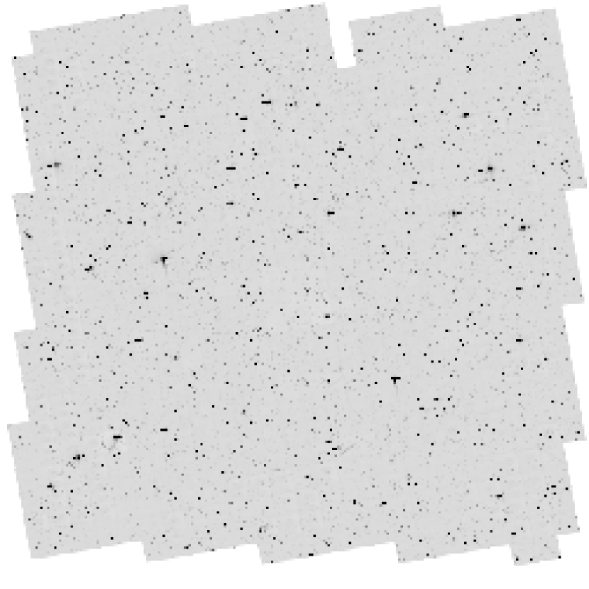
Figure 4: The final combined mosaic of all the ACS pointings. At a pixel scale of $0\farcs 05$/pixel, this image has 100800 pixels on a side ($\sim 84\arcmin$), with the observations covering an area of 1.64 degree². The field is centered at 10:00:28.6, +02:12:21.0 (J2000); the rectangle fully enclosing all the ACS imaging has lower left and upper right corners (RA,DEC J2000) at (150.7988^∘,1.5676^∘) and (149.4305^∘, 2.8937^∘).

Table 1: COSMOS HST ACS/WFC Observations

Range of dates	PA (Deg)	Number of pointings
2003-Oct-15 — 2004-Jan-07	100	42
2004-Mar-02 — 2004-May-21	280	303
2004-Oct-13 — 2005-Jan-07	100	103
2005-Mar-02 — 2005-May-21	280	142
2005-Oct-28 — 2005-Nov-24	100	2

References

- Anderson (2005) Anderson, J. 2005, HST Calibration Workshop, eds. A. M. Koekemoer, P. Goudfrooij, L. L. Dressel (Baltimore: STScI), 11
- Aussel et al. (2007) Aussel, H. et al.2007, ApJS, this volume
- Beckwith et al. (2006) Beckwith, S. V. W., Stiavelli, M., Koekemoer, A. M., Caldwell, J. A. R., Ferguson, H. C., Hook, R., Lucas, R. A., Bergeron, L. E., Corbin, M., Jogee, S., Panagia, N., Robberto, M., Royle, P., Somerville, R. S., Sosey, M. 2006, AJ, 132, 1729
- Capak et al. (2007) Capak, P. et al.2007, ApJS, this volume
- Davis et al. (2006) Davis, M.. et al.. 2006, ApJ, submitted
- Fruchter & Hook (2002) Fruchter, A. S. & Hook, R. N. 2002, PASP, 114, 144
- Giavalisco et al. (2004) Giavalisco, M., Ferguson, H. C., Koekemoer, A. M., Dickinson, M., Alexander, D. M., Bauer, F. E., Bergeron, J., Biagetti, C., Brandt, W. N., Casertano, S., Cesarsky, C., Chatzichristou, E., Conselice, C., Cristiani, S., Da Costa, L., Dahlen, T., de Mello, D., Eisenhardt, P., Erben, T., Fall, S. M., Fassnacht, C., Fosbury, R., Fruchter, A., Gardner, J. P., Grogin, N., Hook, R. N., Hornschemeier, A. E., Idzi, R., Jogee, S., Kretchmer, C., Laidler, V., Lee, K. S., Livio, M., Lucas, R., Madau, P., Mobasher, B., Moustakas, L. A., Nonino, M., Padovani, P., Papovich, C., Park, Y., Ravindranath, S., Renzini, A., Richardson, M., Riess, A., Rosati, P., Schirmer, M., Schreier, E., Somerville, R. S., Spinrad, H., Stern, D., Stiavelli, M., Strolger, L., Urry, C. M., Vandame, B., Williams, R., Wolf, C. 2004, ApJ, 600, 99
- Koekemoer et al. (2002) Koekemoer, A. M., Fruchter, A. S., Hook, R. N. & Hack, W. 2002, HST Calibration Workshop, eds. S. Arribas, A. M. Koekemoer, B. Whitmore (Baltimore: STScI), 337
- Rhodes et al. (2007) Rhodes, J. R. et al.2007, ApJS, this volume
- Rix et al. (2004) Rix, H.-W., Barden, M., Beckwith, S. V. W., Bell, E. F., Borch, A., Caldwell, J. A. R., Häussler, B., Jahnke, K., Jogee, S., McIntosh, D. H., Meisenheimer, K., Peng, C. Y., Sanchez, S. F., Somerville, R. S., Wisotzki, L., Wolf, C. 2004, ApJS, 152, 163
- Schinnerer et al. (2004) Schinnerer, E., Carilli, C. L., Scoville, N. Z., Bondi, M., Ciliegi, P., Vettolani, P., Le Fèvre, O., Koekemoer, A. M., Bertoldi, F., Impey, C. D. 2004, AJ, 128, 1974
- Scoville et al. (2007a) Scoville, N. Z.et al.2007a, ApJS, this volume
- Scoville et al. (2007b) Scoville, N. Z. et al.2007, ApJS, this volume
- Taniguchi et al. (2007) Taniguchi, Y. et al.2007, ApJS, this volume
- Williams et al. (1996) Williams, R. E., Blacker, B., Dickinson, M., Dixon, W. V. D., Ferguson, H. C., Fruchter, A. S., Giavalisco, M., Gilliland, R. L., Heyer, I., Katsanis, R., Levay, Z., Lucas, R. A., McElroy, D. B., Petro, L., Postman, M., Adorf, H.-M., Hook, R. 1996, AJ, 112, 1335
- Williams et al. (2000) Williams, R. E., Baum, S., Bergeron, L. E., Bernstein, N., Blacker, B. S., Boyle, B. J., Brown, T. M., Carollo, C. M., Casertano, S., Covarrubias, R., de Mello, D. F., Dickinson, M. E., Espey, B. R., Ferguson, H. C., Fruchter, A. S., Gardner, J. P., Gonnella, A., Hayes, J., Hewett, P. C., Heyer, I., Hook, R., Irwin, M., Jones, D., Kaiser, M. E., Levay, Z., Lubenow, A., Lucas, R. A., Mack, J., MacKenty, J. W., Madau, P., Makidon, R. B., Martin, C. L., Mazzuca, L., Mutchler, M., Norris, R. P., Perriello, B., Phillips, M. M., Postman, M., Royle, P., Sahu, K., Savaglio, S., Sherwin, A., Smith, T. E., Stiavelli, M., Suntzeff, N. B., Teplitz, H. I., van der Marel, R. P., Walker, A. R., Weymann, R. J., Wiggs, M. S., Williger, G. M., Wilson, J., Zacharias, N., Zurek, D. R. 2000, AJ, 120, 2735