On the effect of helium enhancement on bolometric corrections and $T_{\rm eff}$-colour relations

We evaluate the effects that variations in He content have on bolometric corrections and $T_{\rm eff}$-colour relations. To this aim, we compute ATLAS9 model atmospheres and spectral energy distributions for effective temperatures ranging from 3500 K to 40000 K for dwarfs and from 3500 K to 8000 K for giants, considering both “He-non enhanced” and “He-enhanced” compositions. The considered variations in He content are of $\Delta Y=+0.1$ and $+0.2$ for the metallicity $\mbox{\rm[{\rm M}/{\rm H}]}=+0.5$ and $\Delta Y=+0.1$ for $\mbox{\rm[{\rm M}/{\rm H}]}=-0.5$ and $-1.5$. Then, synthetic photometry is performed in the $UBVRIJHK$ system. We conclude that the changes in bolometric corrections, caused by the adopted He-enhancements are in general too small (less than 0.01 mag), for both dwarfs and giants, to be affecting present-day tables of bolometric corrections at a significant level. The only possible exceptions are found for the $U$-band at $T_{\rm eff}$ between 4000 K and 8000 K, where $|\Delta BC_{U}|$ amounts to $\sim 0.02$ mag, and for $T_{\rm eff}$ equal to 3500 K, where $|\Delta BC_{S_{\lambda}}|$ values become clearly much higher (up to 0.06 mag for passbands from $U$ to $V$). However, even in the latter case the overall uncertainty caused by variations in the He content may be not so significant, because the ATLAS9 results are still approximative at their lowest temperature limit.

1 Introduction

Over the last years, many different problems have prompted the computation of stellar evolutionary tracks for different values of initial He content. Just to mention a few of them:

1) Evidence has been found for significant variations in He content in some globular cluster like $\omega$ Cen, NGC 2808 and M 13 (Piotto et al. 2005; Lee et al. 2005; D’Antona et al. 2005; Caloi & D’Antona 2005). These variations suggest that the relationship between He and metal content was not univocal during the first period of chemical enrichemnt of the universe. A univocal relationship, instead, has so far been assumed in most grids of stellar models applied to the study of old stellar populations.

2) The primordial He content has been recently revised upward, from $Y_{\rm p}\sim 0.235$ to $Y_{\rm p}=0.248\pm 0.001$, after the WMAP mission (Spergel et al. 2003, 2006). Many grids of models for population II stars have been computed for $Y$ values lower than the WMAP one.

3) On one side the helium content in five Hyades binary systems ($Y=0.255$) is lower than expected from their supersolar metallicity, pointing to a value $dY/dZ$ of the order of 1 (Lebreton et al, 2001), whereas other observations either indicate higher values, $dY/dZ\sim 2-2.5$ (e.g Jimenez et al. 2003 from K dwarf stars in the Hipparcos catalog; Peimbert et al. 2002 from extragalactic HII regions), or fail to constrain it to a significant level ($dY/dZ=3\pm 2$, Pagel & Portinari 1998). Grids of stellar models for population synthesis (e.g. Bertelli et al. 1994; Girardi et al 2000), instead, in general use high $dY/dZ$ values in order to fit both the primordial and the solar initial He content.

These aspects have prompted us to start a large project for the computation of stellar tracks covering a large region of the $Y-Z$ plane (Bertelli et al. in preparation). Once ready, these tracks will allow us to model stellar populations at any intermediate $Y$, thus taking into account the changes in lifetimes, luminosities and $T_{\rm eff}$ that follow from a varying $Y$.

However, before stellar evolutionary tracks and isochrones are compared with observations, they have to be converted to magnitudes and colours via bolometric corrections (BC) and colour-$T_{\rm eff}$ relations. The latter may also be affected by the changes in He content, and the purpose of this paper is exactly to evaluate how much. To do so, we first compute energy distributions for a few selected chemical mixtures with different $Y$ (Sect. 2), and then perform synthetic photometry on them (Sect. 3). The results, in terms of changes in BCs and colours, are discussed in Sect. 4.

2 Synthetic spectra for He-enhanced compositions

Small grids of ATLAS9 model atmospheres and energy distributions (Castelli & Kurucz 2003) were generated for different sets of metallicities and enhanced helium contents. For consistency reasons between continuous and line opacities, new opacity distribution functions (ODFs) were computed for each chemical composition having enhanced helium abundance. The DFSYNTHE code (Kurucz 2005; Castelli 2005) was used to this purpose.

The solar and scaled-solar abundances selected for this study are based on the solar chemical composition from Grevesse & Sauval (1998). They are the same ones used by Castelli & Kurucz (2003) for the ODFNEW grids of models and fluxes. In terms of fractional mass, the abundances are $X=0.735,Y=0.248,Z=0.0170$ for the solar case. The solar and scaled-solar abundances will hereafter be mentioned as the $\Delta Y=0$ case. Then, for 3 different values of metal content, we have computed energy distributions for the following mixtures:

• for $\mbox{\rm[{\rm M}/{\rm H}]}=-1.5$: $\Delta Y=0$ and $\Delta Y=0.1$.

• for $\mbox{\rm[{\rm M}/{\rm H}]}=-0.5$: $\Delta Y=0$ and $\Delta Y=0.1$.

• for $\mbox{\rm[{\rm M}/{\rm H}]}=+0.5$: $\Delta Y=0$, $\Delta Y=0.1$ and $\Delta Y=0.2$.

The $\mbox{\rm[{\rm M}/{\rm H}]}=-1.5$ and $\mbox{\rm[{\rm M}/{\rm H}]}=-0.5$ spectra aim to probe the effect of He at globular cluster metallicities, whereas the $\mbox{\rm[{\rm M}/{\rm H}]}=+0.5$ ones serve to probe the potential effect at the supersolar metallicities found in giant ellipticals, for which measurements of the He content do not exist. The effects at solar metallicities are of course derivable by interpolation between the $\mbox{\rm[{\rm M}/{\rm H}]}=-0.5$ and $\mbox{\rm[{\rm M}/{\rm H}]}=+0.5$ cases.

Then, for each one of these chemical mixtures, we compute energy distributions for a sequence of dwarfs and giants at several $T_{\rm eff}$ values. They are:

• Dwarfs: with $\log g=4.5$, and for $T_{\rm eff}$=3500, 4000, 5000, 6000, 8000, 12000, 20000, and 40000 K.

• Giants: with $\log g=1.5$, and for $T_{\rm eff}$=3500, 4000, 5000, 6000, and 8000 K.

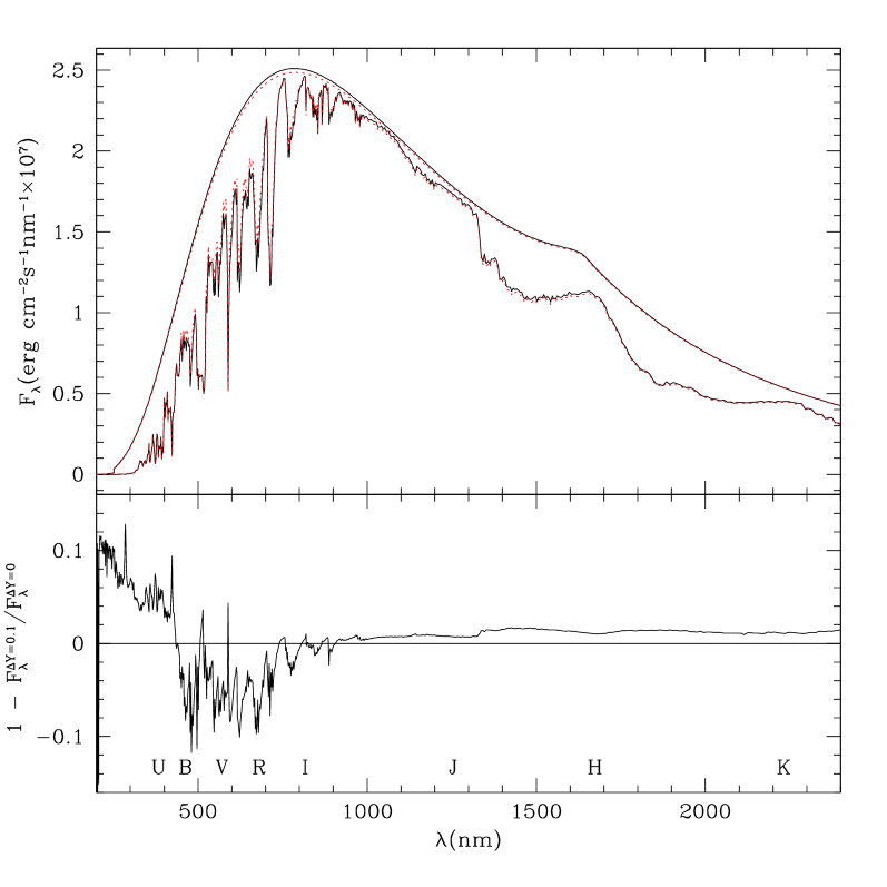
Figure 1: Top panel: Spectral energy distribution for a star with $\mbox{$T_{\rm eff}$}=3500$ K, $\log g=4.5$, and $\mbox{\rm[{\rm M}/{\rm H}]}=-0.5$, for both the $\Delta Y=0$ and $\Delta Y=0.1$ cases (full and dotted lines, respectively). The two upper lines compare the continua, the two lower lines compare the emergent fluxes ($F_{\lambda}^{\Delta Y=0.1}$ and $F_{\lambda}^{\Delta Y=0}$). Bottom panel: the relative difference between the above spectral energy distributions, illustrated by means of $1-F_{\lambda}^{\Delta Y=0.1}/F_{\lambda}^{\Delta Y=0}$. The plot also indicates the approximate location of Johnson-Cousins $UBVRIJHK$ pass-bands.

As an example, Figure 1 compares spectral energy distributions, differing only for the He content, for a relatively cool dwarf of intermediate metallicity. In the top panel, the upper continous lines indicate the emergent flux due to the only continous opacities, while the lower lines are the emergent flux due to both continous and line opacities. The He-enhancement has a modest impact on the emergent spectra. This is evident in the bottom panel of Fig. 1, where the quantity $1-F_{\lambda}^{\Delta Y=0.1}/F_{\lambda}^{\Delta Y=0}$ is plotted. The differences between the two spectra amount to just a few percent, which translate in maximum changes of just a few hundredths of magnitude in bolometric corrections (see Sect. 3 below).

Moreover, some of the differences seen in the bottom panel of Fig. 1 are of no concern because they appear at spectral regions where the emergent flux is very small (for instance, for $\lambda<400$ nm in the figure). In order to better illustrate the differences in the computed spectra which are due only to the variation in the He content, Fig. 2 presents a complete series of plots of the quantity $\delta F_{\lambda}$, defined as

$$\delta F_{\lambda}=\frac{F_{\lambda}^{\Delta Y=0}-F_{\lambda}^{\Delta Y=0.1}}{F_{{\rm max}}^{\Delta Y=0}}$$ (1)

where $F_{{\rm max}}^{\Delta Y=0}$ is the maximum flux of the $F_{\lambda}^{\Delta Y=0}$ spectrum. By plotting the quantity $\delta F_{\lambda}$, we evidence only the differences that occur in the spectral region which is more relevant in terms of flux. This allows a quick evaluation of the changes that are potentially more important to the photometry. Of course, differences between the $\Delta Y=0$ and $\Delta Y>0$ cases occur over the complete range of $\lambda$.

Figure 2: The quantity $\delta F_{\lambda}$ (see eq. 1) as a function of $\lambda$, as derived for the $\mbox{\rm[{\rm M}/{\rm H}]}=-0.5$ spectra with $\Delta Y=0$ and $\Delta Y=0.1$. The top and bottom panels show sequences of decreasing $T_{\rm eff}$ for both dwarfs and giants, respectively. Similar figures are available also for $\mbox{\rm[{\rm M}/{\rm H}]}=-1.5$ and $\mbox{\rm[{\rm M}/{\rm H}]}=+0.5$, and can be provided upon request.

3 Synthetic photometry and results

We have performed synthetic photometry for the above-mentioned energy distributions using the same formalism as in Bessell et al. (1998) and Girardi et al. (2002). Since we are just interested in the changes that the enhanced He can have in the synthetic photometry, the equation to be used is:

$$\Delta BC_{S_{\lambda}}=-2.5\,\log\left(\frac{\int_{\lambda_{1}}^{\lambda_{2}}\lambda F_{\lambda}^{\Delta Y>0}\,S_{\lambda}\mbox{${\rm d}$}\lambda}{\int_{\lambda_{1}}^{\lambda_{2}}\lambda F_{\lambda}^{\Delta Y=0}\,S_{\lambda}\mbox{${\rm d}$}\lambda}\right)$$ (2)

where $S_{\lambda}$ is the total throughput in the filter under consideration, defined in the interval $[\lambda_{1},\lambda_{2}]$. These $\Delta BC_{S_{\lambda}}$ directly tell us the effect of He-enhancement on the absolute magnitudes. The effect on colours can be simply derived by the differences in $\Delta BC_{S_{\lambda}}$ for two filters.

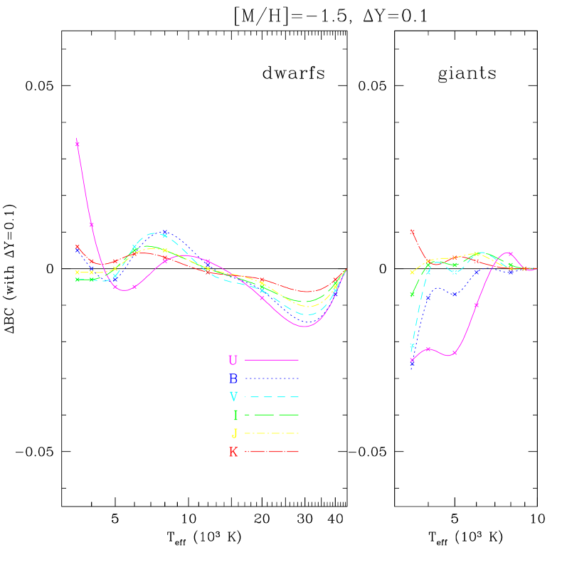
Figure 3: The $\Delta BC_{S_{\lambda}}$ quantities as a function of $T_{\rm eff}$, for both dwarfs and giants of metallicity $\mbox{\rm[{\rm M}/{\rm H}]}=-1.5$ and $\Delta Y=0.1$, and for some of the Johnson-Cousins-Glass $UBVRIJHK$ filters. The small crosses are the $\Delta BC_{S_{\lambda}}$ values effectively computed in this work; they are linked by natural spline curves just for the sake of a better distinction between the different filters.

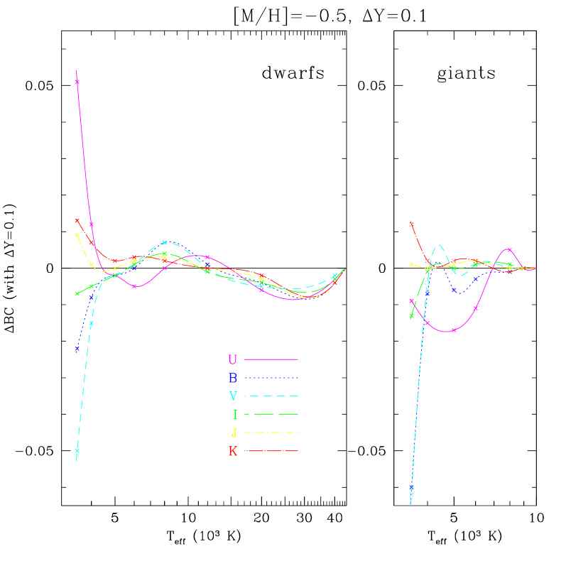
Figure 4: The same as Fig. 3, but for $\mbox{\rm[{\rm M}/{\rm H}]}=-0.5$ and $\Delta Y=0.1$.

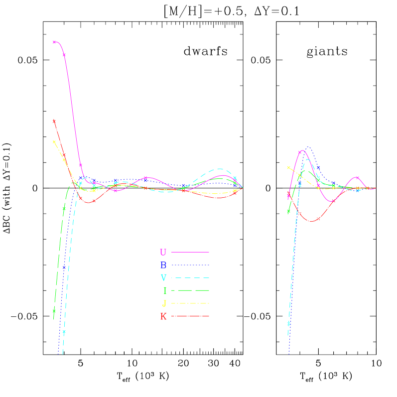
Figure 5: The same as Fig. 3, but for $\mbox{\rm[{\rm M}/{\rm H}]}=+0.5$ and $\Delta Y=0.1$.

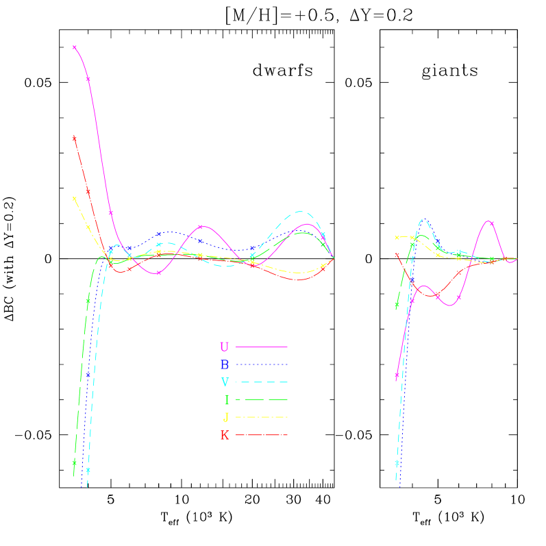
Figure 6: The same as Fig. 3, but for $\mbox{\rm[{\rm M}/{\rm H}]}=+0.5$ and $\Delta Y=0.2.$

Figures 3 to 6 illustrate the behaviour of $\Delta BC_{S_{\lambda}}$ as a function of $T_{\rm eff}$, for both dwarfs and giants, for all [M/H] and $\Delta Y$ values considered in this work, and for the specific case of Johnson-Cousins-Glass $UBVRIJHK$ filters. The filter curves were taken from Bessell (1990) and Bessell & Brett (1988). The same data are tabulated in Table 1, and is provided in electronic form at http://pleiadi.oapd.inaf.it.

4 Discussion and conclusions

As can be readily seen in Figs. 3 to 6, the effect of He-enhancement in the BC is overall quite modest. The most remarkable result for all cases considered here is that $|\Delta BC_{S_{\lambda}}|$ are smaller than 0.009 mag for all stars with $\mbox{$T_{\rm eff}$}\geq 5000$ K and for all pass-bands redder than $U$. The typical $|\Delta BC_{S_{\lambda}}|$ values in these cases are even smaller, of the order of 0.005 mag. In general the corresponding shifts in absolute magnitude are well below the typical errors in photometric observations. Since in most cases the $\Delta BC_{S_{\lambda}}$ behave in a similar way for different filters, the effects in colours are of even smaller magnitude. It is clear to us that the effect of He-enhancement is small enough to be neglected in these cases.

Significant values of $|\Delta BC_{S_{\lambda}}|$ are met just in a few situations; namely for the $U$ filter and at intermediate values of $T_{\rm eff}$  i.e. between 4000 and 8000 K, $|\Delta BC_{S_{\lambda}}|$ become slightly higher but anyway still of the order of 0.02 mag. This is already an effect that could be detected in the (as far as we know, rare) case of high-precision photometry in the $U$ passband. The considered range of $T_{\rm eff}$ is high enough to include the turn-off region of metal-poor globular clusters, and part of their horizontal branch. Therefore, in very specific cases the effect of He-enhancement may have to be considered in globular clusters.

On the other hand for $T_{\rm eff}$ approaching the value of 3500 K and for most filters in the blue part of the spectrum (from $U$ to $V$), $|\Delta BC_{S_{\lambda}}|$ become significantly larger and can amount to as much as 0.06 mag at $\mbox{\rm[{\rm M}/{\rm H}]}\leq-0.5$, and 0.15 mag at $\mbox{\rm[{\rm M}/{\rm H}]}=+0.5$. These low $T_{\rm eff}$ values are those typical of early-M giants, including for instance the tip of the RGB (TRGB) at old ages and moderately low metallicities ($\mbox{\rm[{\rm Fe}/{\rm H}]}\sim-0.7$). Fortunately in the same range of low $T_{\rm eff}$ the red and infrared passbands present small $\Delta BC_{S}$ corrections, in particular in the $I$ band $\Delta BC_{I}$ becomes smaller than $0.015$ mag. We notice that distance determinations of resolved galaxies via the TRGB $I$-band magnitude should not be affected by possible galaxy-to-galaxy changes in the mean He content, since they usually refer to stars hotter than $\sim 4000$ K, for which the possible $\Delta BC_{I}$ corrections are even smaller than at 3500 K.

However, we remark that it is not at all clear whether the significant values of $|\Delta BC_{S_{\lambda}}|$ at $\mbox{$T_{\rm eff}$}\sim 3500$ K are a serious problem owing to the well-known uncertainties of the ATLAS9 models for $\mbox{$T_{\rm eff}$}\leq 4000$ K. For instance, at $\mbox{$T_{\rm eff}$}\sim 3500$ K starts the formation of strong molecular bands in the stellar spectra, which are not accurately reproduced – at least not at the level of a few percent – by present-day ATLAS9 models (see for instance Fluks et al. 1994). Among the reasons there is the lack in the line opacity computations of both triatomic molecules (with exception for H₂O which is considered) and of numerous diatomic molecular transitions.

Therefore, the significant changes in $\Delta BC_{S_{\lambda}}$ that we find at low $T_{\rm eff}$ may be just one additional – and secondary – problem in a field that is already complicated in itself, and for which synthetic photometry has always been recognized not to provide accurate answers.

In conclusion, we find that the effects of changes in He abundances among stellar populations are quite modest when we look at the stellar atmospheres and their predicted bolometric corrections. Therefore, the use of tables of BCs computed for a single $Y(Z)$ relation, is an acceptable approximation in most cases. We provide tables for $\Delta BC_{S_{\lambda}}$ in a series of [M/H], $\Delta Y$, and $T_{\rm eff}$ values, that may help the reader to evaluate whether this is an issue in the interpretation of their observations. The effects of changing $Y$ by as much as 0.1, instead, may have a quite high impact on the stellar evolutionary tracks, and have to be considered whenever it is suspected, as in the case of $\omega$ Cen.

References

Bertelli, G., et al., 1994, A&AS, 106, 275

Bessell, M.S., 1990, PASP, 102, 1181

Bessell, M.S., & Brett J.M., 1988, PASP, 100, 1134

Bessell, M.S., Castelli F., & Plez B., 1998, A&A. 333, 231

Caloi, V., & D’Antona, F., 2005, A&A, 435, 987

Castelli, F., 2005, MSAIS, 8, 34

Castelli, F., Gratton, R.G., & Kurucz R.L., 1997, A&A, 318, 841

Castelli, F., & Kurucz, R. L., 2003, IAU Symposium, 210, 20P

D’Antona, F. et al., 2005 ApJ, 631, 868

Fluks, M.A, Plez, B., The, P.S., et al., 1994, A&AS, 105, 311

Girardi, L., Bressan, A., Bertelli, G., Chiosi, C., 2000, A&AS, 141,371

Grevesse, N., & Sauval, A. J., 1998, SSR 85, 161

Jimenez, R. et al., 2003, Science, 299, 1552

Kurucz, R.L., 1993, in IAU Symp. 149: The Stellar Populations of Galaxies, eds. B. Barbuy, A. Renzini, Dordrecht, Kluwer, p. 225

Kurucz, R. L,. 2005, MSAIS, 8, 14

Lebreton, Y. et al.., 2001, A&A, 374, 540

Lee, Y.-W., et al., 2005, ApJ, 621, L57

Pagel, B.E.J., & Portinari, L., 1998, MNRAS,298,747

Peimbert, M. et al. ., 2000, ApJ, 541, 688

Piotto, G., et al., 2005, ApJ, 621, 777

Spergel, D.N., et al., 2003, ApJS, 148, 175

Spergel, D.N., et al., 2006, astro-ph/0603449

[x]rr—rrrrrrrrr $\Delta BC_{S_{\lambda}}$ values (in mag) for the $UBVRIJHK$ system of Bessell (1990) and Bessell & Brett (1988).
$T_{\rm eff}$ $\log g$ $U$ $BX$ $B$ $V$ $R$ $I$ $J$ $H$ $K$
continued.
$T_{\rm eff}$ $\log g$ $U$ $BX$ $B$ $V$ $R$ $I$ $J$ $H$ $K$
$\mbox{\rm[{\rm M}/{\rm H}]}=-1.5,\Delta Y=0.1$
3500 4.50 0.034 0.005 0.005 -0.003 -0.006 -0.003 -0.001 0.000 0.006
4000 4.50 0.012 0.000 0.000 -0.003 -0.004 -0.003 -0.001 0.001 0.002
5000 4.50 -0.005 -0.003 -0.003 -0.002 -0.001 0.000 0.000 0.002 0.002
6000 4.50 -0.005 0.004 0.004 0.006 0.005 0.005 0.004 0.005 0.004
8000 4.50 0.002 0.010 0.010 0.009 0.007 0.005 0.005 0.003 0.003
12000 4.50 0.002 0.001 0.001 -0.001 0.000 0.000 0.000 0.000 -0.001
20000 4.50 -0.008 -0.006 -0.006 -0.006 -0.005 -0.005 -0.004 -0.003 -0.003
40000 4.50 -0.007 -0.007 -0.007 -0.006 -0.004 -0.004 -0.005 -0.005 -0.003
3500 1.50 -0.025 -0.027 -0.026 -0.021 -0.014 -0.007 -0.001 0.009 0.010
4000 1.50 -0.022 -0.008 -0.008 -0.001 0.000 0.001 0.002 0.001 0.002
5000 1.50 -0.023 -0.007 -0.007 -0.001 0.002 0.001 0.003 0.004 0.003
6000 1.50 -0.010 -0.001 -0.001 0.004 0.004 0.004 0.004 0.002 0.002
8000 1.50 0.004 -0.001 -0.001 0.000 0.000 0.001 0.000 -0.001 0.000
$\mbox{\rm[{\rm M}/{\rm H}]}=-0.5,\Delta Y=0.1$
3500 4.50 0.051 -0.024 -0.022 -0.050 -0.044 -0.007 0.009 0.014 0.013
4000 4.50 0.012 -0.008 -0.008 -0.015 -0.014 -0.005 0.001 0.008 0.007
5000 4.50 -0.002 -0.002 -0.002 -0.002 -0.002 -0.002 0.000 0.002 0.002
12000 4.50 0.003 0.001 0.001 0.000 0.000 -0.001 0.000 0.000 0.000
20000 4.50 -0.006 -0.005 -0.004 -0.005 -0.004 -0.004 -0.003 -0.003 -0.002
40000 4.50 -0.003 -0.004 -0.004 -0.002 -0.002 -0.003 -0.004 -0.004 -0.004
3500 1.50 -0.009 -0.061 -0.060 -0.062 -0.037 -0.013 0.001 0.009 0.012
4000 1.50 -0.015 -0.007 -0.007 -0.004 -0.003 -0.001 0.000 0.002 0.002
5000 1.50 -0.017 -0.005 -0.006 -0.001 0.000 0.000 0.001 0.002 0.002
6000 1.50 -0.011 -0.002 -0.003 0.001 0.002 0.001 0.002 0.001 0.002
8000 1.50 0.005 -0.001 -0.001 0.000 0.000 0.001 0.000 0.000 -0.001
$\mbox{\rm[{\rm M}/{\rm H}]}=+0.5,\Delta Y=0.1$
3500 4.50 0.057 -0.096 -0.092 -0.130 -0.088 -0.048 0.018 0.034 0.026
4000 4.50 0.052 -0.032 -0.031 -0.056 -0.047 -0.008 0.011 0.013 0.013
5000 4.50 0.009 0.004 0.004 0.002 0.001 0.000 0.000 -0.004 -0.004
6000 4.50 0.002 0.003 0.003 0.001 0.000 0.000 -0.001 -0.004 -0.005
8000 4.50 -0.001 0.003 0.003 0.002 0.002 0.001 0.001 0.000 0.001
12000 4.50 0.004 0.002 0.003 0.000 0.000 0.000 0.000 0.001 0.000
20000 4.50 -0.001 0.001 0.001 0.000 0.000 0.000 -0.001 -0.001 -0.001
40000 4.50 0.003 0.001 0.001 0.004 0.003 0.002 -0.001 -0.002 -0.002
3500 1.50 -0.003 -0.067 -0.067 -0.053 -0.010 -0.009 0.008 -0.002 -0.002
4000 1.50 0.014 0.002 0.002 0.001 0.003 0.005 0.005 -0.008 -0.010
5000 1.50 0.001 0.008 0.008 0.004 0.004 0.003 0.000 -0.009 -0.012
6000 1.50 -0.005 0.002 0.002 0.001 0.002 0.001 0.000 -0.004 -0.005
8000 1.50 0.004 -0.001 -0.001 -0.001 0.000 0.000 0.000 0.000 0.000
$\mbox{\rm[{\rm M}/{\rm H}]}=+0.5,\Delta Y=0.2$
3500 4.50 0.060 -0.107 -0.103 -0.147 -0.102 -0.058 0.017 0.042 0.034
4000 4.50 0.051 -0.035 -0.033 -0.060 -0.052 -0.012 0.009 0.019 0.019
5000 4.50 0.013 0.004 0.003 0.002 -0.001 -0.001 0.000 -0.002 -0.002
6000 4.50 0.001 0.003 0.003 0.001 0.000 0.000 0.000 -0.002 -0.003
8000 4.50 -0.004 0.006 0.007 0.004 0.003 0.001 0.002 0.000 0.001
12000 4.50 0.009 0.005 0.005 0.000 0.001 0.001 0.001 0.002 0.000
20000 4.50 -0.002 0.003 0.003 0.001 0.000 0.000 -0.001 -0.001 -0.002
40000 4.50 0.006 0.004 0.004 0.007 0.006 0.004 -0.002 -0.003 -0.003
3500 1.50 -0.033 -0.081 -0.081 -0.058 -0.014 -0.013 0.006 -0.002 0.001
4000 1.50 -0.012 -0.006 -0.006 0.000 0.002 0.004 0.006 -0.007 -0.007
5000 1.50 -0.011 0.005 0.005 0.004 0.004 0.003 0.001 -0.007 -0.010
6000 1.50 -0.011 0.002 0.001 0.002 0.002 0.001 0.000 -0.003 -0.004
8000 1.50 0.010 -0.001 -0.001 -0.001 0.000 0.000 -0.001 -0.001 -0.001