Coulomb Bubbles: Over-stable driving of Magnetoacoustic Waves due to the Rapid and Anisotropic Diffusion of Energy

Abstract

We perform a linear magnetohydrodynamic perturbation analysis for a stratified magnetized envelope where the diffusion of heat is mediated by charged particles that are confined to flow along magnetic field lines. We identify an instability, the “coulomb bubble instability,” which may be thought of as standard magnetosonic fast and slow waves, driven by the rapid diffusion of heat along the direction of the magnetic field. We calculate the growth rate and stability criteria for the coulomb bubble instability for various choices of equilibrium conditions.

The coulomb bubble instability is intimately related to the photon bubble instability. The bulk thermodynamic properties of both instability mechanisms are quite similar in that they require the timescale for heat to diffuse across a wavelength to be shorter than the corresponding wave-crossing time. Furthermore, over-stability occurs only as long as the driving resulting from the presence of the background heat flux can overcome diffusive Silk damping. However, the geometric and therefore mechanical properties of the coulomb bubble instability is the complete mirror opposite of the photon bubble instability.

The coulomb bubble instability is most strongly driven for weakly magnetized atmospheres that are strongly convectively stable. We briefly discuss a possible application of astrophysical interest: diffusion of interstellar cosmic rays in the hot $T\sim 10^{6}$ K Galactic corona. We show that for commonly accepted values of the cosmic ray and gas pressure as well as its overall characteristic dimensions, the Galactic corona is in a marginal state of stability with respect to a cosmic ray coulomb bubble instability. The implication being that a cosmic ray coulomb bubble instability plays a role regulating both the pressure and transport properties of interstellar cosmic rays, while serving as a source of acoustic power above the galactic disk.

1 Introduction

The idea that the diffusive flow of energy up through an atmosphere carries with it, the potential to de-stabilize acoustic motion, has been considered for quite some time (Baker & Kippenhahn 1962). The most familiar situation is where the flow of energy is transmitted by a radiative heat flux and the instability mechanism operates due to changes in the opacity that result from nearly adiabatic changes in temperature and density, along the wave. The instability mechanism, known as the $\kappa$-mechanism, is responsible for the strong observed pulsations in RR-Lyrae and Cepheid variable stars.

In the case where the instability is strong such that the pulsation amplitude is large, the overall structure and evolution of the equilibrium flow may be significantly altered. If the saturation amplitude is small, information on the overall structure of the system may be extracted.

More recently, the inclusion of magnetic fields into perturbation analyses of optically thick, radiating, stratified flows has produced some interesting results. In particular, accretion flows onto black holes and neutron stars are unstable to the photon bubble instability (Arons 1992; Gammie 1998; Blaes & Socrates 2001). Furthermore, the photon bubble instability, which can be thought of as a standard magnetosonic wave that is driven over-stable by the presence of a stratified radiation field, may operate in equilibria that are weakly magnetized and/or highly sub-Eddington (Blaes & Socrates 2003).

Balbus (2001) showed that incompressible Brunt-Vaisalla oscillations are unstable when horizontally-separated fluid elements are thermally-connected by coulomb conduction along field lines of relatively little dynamical importance. This “magneto-thermal instability” operates as long as the diffusion of heat along the field lines is rapid in comparison to the Brunt-Vaisalla frequency. For sufficiently weak fields, instability occurs for atmospheres with an outward decreasing temperature profile, rather than an outward decreasing entropy profile – as in the case of convective stability (see e.g. Parrish & Stone 2005; Chandran & Dennis 2006).

In this work we explore the possibility that magnetoacoustic waves may be secularly driven when the envelope’s flux of heat is mediated by anisotropic thermal diffusion that occurs solely along magnetic field lines. The stability of magnetized neutron stars, cosmic ray diffusion in the interstellar medium and the thermal structure of cluster-scale cooling flows are some examples of where the following instability analysis may be be relevant.

The plan of this work is as follows. In §2 we express our basic assumptions, write down the necessary conservation laws and then specify the parameters of the simple equilibria, which we then perturb. Furthermore, in §2.2 we place our analysis within the context of previous work on linear MHD theory where the effects of rapid heat diffusion was taken into account. In §3 our linear analysis begins, with an emphasis on the thermodynamics of the coulomb bubble instability. In §4, our linear analysis continues with an emphasis on the mechanics of the coulomb bubble instability. In §4.4, we present a physical description of the coulomb bubble driving mechanism in juxtaposition with the photon bubble instability. In §5, we discuss the possibility that the Coulomb Bubble instability might play a role in determining the nature of interstellar cosmic ray diffusion. In §6 we summarize our results and discuss possibilities for further research.

2 Assumptions, Fundamental Equations and Perturbations

2.1 Conservation Laws and the Background

We assume that the basic equations of ideal MHD apply. Also, the only source term in the first law of thermodynamics is provided by a diffusive heat flux. The conservation laws given below are the same as those found in Balbus (2001); they are

$$\frac{\partial\rho}{\partial t}+\hbox{{\syvec\char 114\relax}}\cdot\left(\rho{\bf v}\right)=0$$ (1)

$$\rho\left(\frac{\partial{\bf v}}{\partial t}+{\bf v}\cdot\hbox{{\syvec\char 114\relax}}{\bf v}\right)=-\hbox{{\syvec\char 114\relax}}P+\rho\,{\bf g}+\frac{1}{4\pi}\left(\hbox{{\syvec\char 114\relax}}\times{\bf B}\right)\times{\bf B},$$ (2)

$$\rho\,T\left(\frac{\partial s}{\partial t}+{\bf v}\cdot\hbox{{\syvec\char 114\relax}}s\right)=-\hbox{{\syvec\char 114\relax}}\cdot{\bf Q},$$ (3)

$${\bf Q}=-\chi{\hat{\bf b}}{\hat{\bf b}}\cdot\hbox{{\syvec\char 114\relax}}T,$$ (4)

$$\frac{\partial{\bf B}}{\partial t}=\hbox{{\syvec\char 114\relax}}\times\left({\bf v}\times{\bf B}\right),$$ (5)

and

$$\hbox{{\syvec\char 114\relax}}\cdot{\bf B}=0.$$ (6)

Eqs. (1)-(3) enforce conservation of mass, momentum, and energy, respectively while eq. (5) enforces magnetic flux-freezing. Furthermore, eq. (4) constrains that the flow of heat follows a diffusion law along magnetic field lines and eq. (6) enforces ${\bf B}$ to be purely solenoidal. Definitions of the various symbols in the expressions above, as well as others used throughout, are listed in Table 1.

Table 1: Definitions of highly-used symbols

Symbol	Quantity
$\rho$	density
${\bf v}$	velocity
$P$	pressure
$T$	temperature
$s$	entropy per unit mass
${\bf B}$	magnetic flux density
$\hat{\bf b}$	magnetic field unit vector
${\bf Q}$	heat flux
$\chi$	thermal conductivity along field lines
${\bf g}$	gravitational acceleration
$\omega$	wave frequency
${\bf k}$	wave vector
$c_{i}$	isothermal sound speed
${\bf v_{A}}$	Alfvén velocity
$\kappa$	opacity
$\omega_{\rm C,diff}$	$\omega+i\frac{\chi\left({\bf k}\cdot\hat{\bf b}\right)^{2}}{n\,T\,\left(\partial s/\partial T\right)_{\rho}}$
${\tilde{\omega}}^{2}$	$\omega^{2}-\left({\bf k}\cdot{\bf v_{A}}\right)^{2}$
$\xi$	Lagrangian displacement
$\Delta=\delta+\xi\cdot\nabla$	Lagrangian variation
$A_{0}$	asymptotic (in $k$) growthrate
$\delta{\bf Q}_{\perp}$	Eulerian heat flux perturbation $\perp{\bf B}$

The form of the heat flux given by eq. (4) is valid as long as two conditions are satisfied. First, the Larmor radius must be small in comparison to the mean free path of the particles endowed with relatively large amounts thermal mobility and therefore, ${\bf Q}\parallel\hat{\bf b}$. Second, the mean free path along ${\bf B}$ must be smaller than the characteristic scales of the problem e.g., the temperature scale height. Later on, when we consider perturbations, the mean free path along the ${\bf B}$ must be smaller than the wavelength of the perturbation in question.

We assume that the background is in hydrostatic balance and the equilibrium magnetic field ${\bf B}$ is a constant. We have

$$-\frac{1}{\rho}\hbox{{\syvec\char 114\relax}}P={\bf g},$$ (7)

where changes in the gas pressure $P$ are related to changes in density and temperature via an equation of state

$$P=\frac{\rho\,k_{B}T}{\mu m_{p}}.$$ (8)

Throughout, we assume that the mean molecular weight $\mu$ is a constant so that changes in composition are ignored. We only consider a background that may be characterized as a “stellar envelope.” That is, both the surface gravity and thermal energy flux throughout the medium is set to be a constant. In order to resemble a stellar envelope, the condition for radiative equilibrium must read

$$\hbox{{\syvec\char 114\relax}}\cdot{\bf Q}=0$$ (9)

and in addition, the mass of the atmosphere must be insignificant in comparison to the source of the gravitational field.

2.2 Nature of Perturbations in Different Regimes

Our background is simple and closely resembles a basic stellar atmosphere, threaded by an equilibrium magnetic field. The only major difference is that energy does not flow upwards via radiative diffusion, directly against the pull of gravity. Instead, the transfer of energy is mediated by charged particles of relatively high thermal mobility that drift along the equilibrium field.

Now we consider dynamical fluctuations. To keep things simple, we examine local WKB perturbations whose time and spatial dependence are $\propto e^{i\left({\bf k}\cdot{\bf x}-\omega t\right)}$. Furthermore, we only consider wavevectors that are two dimensional i.e., ${\bf k}=(k_{x},k_{z})$, where $\hat{\bf z}$ lies in the vertical direction.

2.2.1 Adiabatic Fluctuations: Alfvèn, Gravity and Magnetosonic Waves

In the limit of slow thermal diffusion, linear perturbations to the first law of thermodynamics, eq. (3), take on a simple form

$$-i\omega\rho T\left(\delta s+\hbox{{\gkvec\char 24\relax}}\cdot\hbox{{\syvec\char 114\relax}}s\right)=-i\omega\rho T\Delta s\simeq 0.$$ (10)

The Eulerian component of $\Delta s$ leads to the fluid’s acoustic response for short-wavelength perturbations, while the Lagrangian component $\propto\hbox{{\gkvec\char 24\relax}}\cdot\hbox{{\syvec\char 114\relax}}s$ leads to the incompressible gravity waves.

Including magnetic forces, compressible (${\bf k}\cdot\delta{\bf v}\neq 0$) short-wavelength perturbations obey the magnetosonic dispersion relation given by

$$\omega^{2}=k^{2}\,c^{2}_{s}\frac{{\tilde{\omega}}^{2}}{\omega^{2}}+k^{2}v^{2}_{A},$$ (11)

where $c_{s}$ is the adiabatic sound speed and all other symbols are defined in Table 1. The eigenvectors corresponding to the roots of the dispersion relation above are referred to as the fast and slow magnetosonic waves.

Incompressible perturbations, with ${\bf k}\cdot\delta{\bf v}=0$, satisfy the dispersion relation

$${\tilde{\omega}}^{2}-\frac{k^{2}_{x}}{k^{2}}N^{2}_{BV}=0$$ (12)

where $N^{2}_{BV}$ is the Brunt-Vaisalla frequency. Basically, the restoring force is provided by a combination of Alfvénic tension and buoyancy.

2.2.2 Highly Non-Adiabatic Incompressible Fluctuations: Balbus’ 2001 Analysis

The fluctuations mentioned above are quite standard and do not therefore, merit further analysis or discussion. Interesting physical effects, such as damping and instability, occur when fluctuations with respect to the flow of matter and the flow of heat separate from one another i.e., when the perturbations become non-adiabatic. Somewhat counter-intuitively, non-adiabatic effects occur when the time scale for heat flow over a wavelength is shorter than the oscillation period of the perturbation in question. That is, the flow becomes non-adiabatic once the agent of heat transfer can either inject into, or remove energy from, the flow before the fluid has time to respond.

Balbus (2001) studied incompressible waves (${\bf k}\cdot\delta{\bf v}=0$ and $c_{s}\rightarrow\infty$) in the limit where the diffusion time along the magnetic field is short in comparison to the wave crossing time. Another condition for Balbus’ (2001) instability is that the Alfvén time must be shorter than the wave crossing time so that Alfvénic tension cannot suppress the unstable growth of the perturbations. He found that Brunt-Vaisalla oscillations (or g-modes) are driven unstable if horizontally-separated fluid elements can quickly transfer heat from regions of relatively high to low temperatures, once they are perturbed in opposite directions along the background temperature gradient. The role of the magnetic field in this “magneto-thermal instability” is to serve as conduit of thermal energy between horizontally-separated fluid elements.

2.2.3 Highly Non-Adiabatic Compressible Fluctuations: This work

We now consider the manner in which compressible (slow and fast) magnetosonic waves are affected by the rapid flow of heat along magnetic field lines. In a sense, the instability and damping mechanisms covered in the next few sections can be viewed as a natural extension of either Balbus’ (2001) or Blaes & Socrates’ (2003) analysis of magnetoacoustic waves driven by the rapid diffusion of heat along the radiation pressure gradient.

3 Total Pressure Perturbation in the Limit of Rapid Heat Conduction

The rapid diffusion of heat alters standard magnetoacoustic motion through the pressure perturbation, which we write as

$$\delta P=\left(\frac{\partial P}{\partial\rho}\right)_{T}\delta\rho+\left(\frac{\partial P}{\partial\,T}\right)_{\rho}\delta T.$$ (13)

That is, we assume that the fluid’s pressure is a function of of $\rho$ and $T$ only such that $P=P(\rho,T)$. Furthermore, $\left({\partial P}/{\partial\rho}\right)_{T}=c^{2}_{i}$ where $c_{i}$ is the isothermal sound speed. For short-wavelength magnetosonic motion, $\delta\rho$ is constrained by the linearized expression for conservation of mass, while $\delta T$ is constrained by the linearized first law of thermodynamics, which reads

$$-i\,\omega\,n\,T\left(\delta s+\hbox{{\gkvec\char 24\relax}}\cdot\hbox{{\syvec\char 114\relax}}s\right)=-i{\bf k}\cdot\delta{\bf Q},$$ (14)

where $s$ and $\delta{\bf Q}$ is the specific entropy and the perturbed coulombic heat flux, respectively. Later on, we show that the manner in which $\delta{\bf Q}$ responds to changes in magnetofluid variables ultimately determines the nature of the various driving and damping mechanisms. Below, we carefully discuss the form of $\delta{\bf Q}$.

3.1 The Heat Flux Perturbation

The equilibrium coulombic heat flux is given by

$${\bf Q}=-\chi\hat{\bf b}\hat{\bf b}\cdot\hbox{{\syvec\char 114\relax}}T=-{\bf X}\cdot\hbox{{\syvec\char 114\relax}}T.$$ (15)

Here, $\chi$ is the conductivity along field lines which lie in the direction ${\bf B}/B=\hat{\bf b}$ and ${\bf X}={\bf X}(\chi,\hat{\bf b})$ is the thermal conductivity tensor. Upon perturbation, we have

$$\delta{\bf Q}=-\delta{\bf X}\cdot\hbox{{\syvec\char 114\relax}}T-{\bf X}\cdot\hbox{{\syvec\char 114\relax}}\delta T=-\chi\left[\frac{\delta\chi}{\chi}\hat{\bf b}\left(\hat{\bf b}\cdot\hbox{{\syvec\char 114\relax}}T\right)+\delta\hat{\bf b}\left(\hat{\bf b}\cdot\hbox{{\syvec\char 114\relax}}T\right)+\hat{\bf b}\left(\delta\hat{\bf b}\cdot\hbox{{\syvec\char 114\relax}}T\right)+i\,\hat{\bf b}\left({\bf k}\cdot\hat{\bf b}\right)\delta T\right]$$ (16)

where the coulombic conductivity $\chi$ is not taken to be a constant. We choose to parameterize the conductivity $\chi$ in the following way,

$$\chi=\chi_{0}T^{n}\rho^{m}\kappa^{p}$$ (17)

where $\chi_{0}$ is a constant and $\kappa$ may be thought of as an “opacity” or in other words, a cross section per unit mass. Comparison with thermally diffusive damping and driving mechanisms for backgrounds in which radiation mediates the flow of energy is facilitated if we choose $n=3$, $m=-1$, and $p=-1$ as in the case of radiative diffusion. In a way, we absorb the micro-physical differences (such as cross section) between radiative and coulombic diffusion into an opacity law – or a mean free path – for the particles that possess relatively large amounts of thermal mobility.

From the above considerations, the expression for the conductivity perturbation is given by

$$\frac{\delta\chi}{\chi}=-\frac{\delta\rho}{\rho}+3\frac{\delta T}{T}-\frac{\delta\kappa}{\kappa}.$$ (18)

For now, we somewhat artificially set $\delta\kappa=0$, which momentarily prevents us from studying a potential $\kappa-$mechanism that results from coulomb diffusion. With this, the expression for the heat flux perturbation becomes

$$\delta{\bf Q}=-\chi\left[-\frac{\delta\rho}{\rho}\,\hat{\bf b}\left(\hat{\bf b}\cdot\hbox{{\syvec\char 114\relax}}T\right)+\delta\hat{\bf b}\left(\hat{\bf b}\cdot\hbox{{\syvec\char 114\relax}}T\right)+\hat{\bf b}\left(\delta\hat{\bf b}\cdot\hbox{{\syvec\char 114\relax}}T\right)+i\,\hat{\bf b}\left({\bf k}\cdot\hat{\bf b}\right)\delta T\right].$$ (19)

Note that we have dropped the term in $\delta\chi\propto 3\,\delta T$ since it contributes at a lower order in $(kH)^{-1}$ relative to the last term in the above expression, within the context of our WKB approximation. We do this with hindsight earned from Blaes & Socrates’ (2003) analysis. The rapid diffusion (high-$k$ limit) of heat along temperature gradients necessarily implies that the temperature perturbation is relatively small by a factor of $1/k$ in comparison perturbations of other magnetofluid quantities such as $\delta\rho$, $\delta\hat{\bf b}$ and $\delta{\bf v}$.

3.2 The Temperature Perturbation

By expanding eq. (14), the first law of thermodynamics, with the help of the expression for the heat flux perturbation $\delta{\bf Q}$ given by eq. (19), we have

$$-\omega\,n\,T\left[\left(\frac{\partial s}{\partial\rho}\right)_{T}\delta\rho+\left(\frac{\partial s}{\partial\,T}\right)_{\rho}\delta\,T+\hbox{{\gkvec\char 24\relax}}\cdot\hbox{{\syvec\char 114\relax}}s\right]=\chi\left[-\frac{\delta\rho}{\rho}\left({\bf k}\cdot\hat{\bf b}\right)\left(\hat{\bf b}\cdot\hbox{{\syvec\char 114\relax}}T\right)+\left({\bf k}\cdot\delta\hat{\bf b}\right)\left(\hat{\bf b}\cdot\hbox{{\syvec\char 114\relax}}T\right)+\left({\bf k}\cdot\hat{\bf b}\right)\left(\delta\hat{\bf b}\cdot\hbox{{\syvec\char 114\relax}}T\right)+i\left({\bf k}\cdot\hat{\bf b}\right)^{2}\delta T\right]$$ (20)

It is useful to define a characteristic diffusion frequency, $\omega_{\rm C,diff}$, which quantifies the rate at which heat diffuses over a wavelength,

$$\omega_{\rm C,diff}\equiv\omega+i\frac{\chi\left({\bf k}\cdot\hat{\bf b}\right)^{2}}{n\,T\,\left(\partial s/\partial T\right)_{\rho}}.$$ (21)

With this, we temperature perturbation becomes

$$\delta T=-\frac{\omega}{\omega_{\rm C,diff}}\frac{\left(\partial s/\partial\rho\right)_{T}}{\left(\partial s/\partial T\right)_{\rho}}\delta\rho-\frac{\omega}{\omega_{\rm C,diff}}\frac{\hbox{{\gkvec\char 24\relax}}\cdot\hbox{{\syvec\char 114\relax}}s}{\left(\partial s/\partial T\right)_{\rho}}-\frac{\chi\left[-\frac{\delta\rho}{\rho}\left({\bf k}\cdot\hat{\bf b}\right)\left(\hat{\bf b}\cdot\hbox{{\syvec\char 114\relax}}T\right)+\left({\bf k}\cdot\delta\hat{\bf b}\right)\left(\hat{\bf b}\cdot\hbox{{\syvec\char 114\relax}}T\right)+\left({\bf k}\cdot\hat{\bf b}\right)\left(\delta\hat{\bf b}\cdot\hbox{{\syvec\char 114\relax}}T\right)\right]}{\omega_{\rm C,diff}\,n\,T\left(\partial s/\partial T\right)_{\rho}}.$$ (22)

By knowing beforehand that the magnetosonic waves of interest can be treated to lowest order as standard fast and slow magnetoacoustic waves tells us that $\omega\simeq v_{\rm ph}\,k$, where $v_{\rm ph}$ is the phase velocity of the given wave. Therefore, in the rapidly diffusing limit,

$$|\omega_{\rm C,diff}|\rightarrow\frac{\chi\left({\bf k}\cdot\hat{\bf b}\right)^{2}}{n\,T\left(\partial s/\partial T\right)_{\rho}}\gg\omega.$$ (23)

Now, the temperature perturbation reduces to

$$\delta T \simeq \frac{i}{\left({\bf k}\cdot\hat{\bf b}\right)^{2}}\left[\frac{n\,\rho\,T\omega}{\chi}\left(\frac{\partial s}{\partial\rho}\right)_{T}\frac{\delta\rho}{\rho}-\frac{\delta\rho}{\rho}\left({\bf k}\cdot\hat{\bf b}\right)\left(\hat{\bf b}\cdot\hbox{{\syvec\char 114\relax}}T\right)+\left({\bf k}\cdot\delta\hat{\bf b}\right)\left(\hat{\bf b}\cdot\hbox{{\syvec\char 114\relax}}T\right)+\left({\bf k}\cdot\hat{\bf b}\right)\left(\delta\hat{\bf b}\cdot\hbox{{\syvec\char 114\relax}}T\right)\right]$$ (24)

The form of the temperature perturbation given by eq. (24) is remarkably similar to the case of rapid radiative diffusion, which potentially leads to photon bubble-like phenomena i.e.,

$$\delta T \simeq \frac{i}{\,k^{2}}\left[\frac{n\,\rho\,T\omega}{\chi}\left(\frac{\partial s}{\partial\rho}\right)_{T}\frac{\delta\rho}{\rho}-\frac{\delta\rho}{\rho}\,\left({\bf k}\cdot\hbox{{\syvec\char 114\relax}}T\right)\right]\,\,\,\,\,\,\,\,{\rm RADIATIVE\,\,\,\,DIFFUSION}.$$ (25)

In both cases, the first term which is $\propto\left(\partial s/\partial\rho\right)_{T}$ leads to diffusive thermal damping. For the specialized case of radiative diffusion, this effect is known as Silk damping (Silk 1968; Weinberg 1971). The remaining terms in eq. (24) and eq. (25) – the one that contain gradients in temperature – lead to secular over-stable driving. For photon bubbles driven by rapid radiative diffusion, the term $\propto{\bf k}\cdot\hbox{{\syvec\char 114\relax}}T\,\delta\rho/\rho$ in the temperature perturbation represents “shadowing” or “pile up.” More specifically, immediately downstream a density maximum, radiation piles up due to the local increase in extinction and since photon number is conserved, a deficit of radiation, or a shadow, occurs. Thus, the resulting radiation pressure differential across the density maxima allows for the possibility of work being performed on the fluid by the radiation field. In the case of anisotropic coulomb conductivity, a local change in the orientation of the magnetic field either permits or deters the flow of heat across a local density maximum. The orientation of $\delta\hat{\bf b}$ relative to constant density surfaces (that are $\perp{\bf k}$) ultimately determine whether or not the change in heat flow drives or damps the oscillation.

It follows that the total pressure perturbation is divided into two parts; one which yields a standard acoustic response $\propto\delta\rho$ while the other component $\propto i\,k^{-1}\delta\rho$ leads to conductive driving and damping. That is,

$$\delta P=\delta P_{\rm ac}+\delta{\tilde{P}}$$ (26)

where

$$\delta P_{\rm ac}=\left(\frac{\partial P}{\partial\rho}\right)_{T}\,\delta\rho=c^{2}_{i}\delta\rho\,\,\,\,\,\,\, {\rm and} \,\,\,\,\,\,\,\delta{\tilde{P}}=\left(\frac{\partial P}{\partial T}\right)_{\rho}\,\delta T.$$ (27)

4 Coupling of Magnetosonic Motion to the Background Coulomb Flux

In what follows, we calculate the growth rates and stability criteria for the fast and slow coulomb bubble instability. We start with a brief overview of standard magnetosonic waves, where background gradients are ignored. We derive the basic properties and reveal the nature of the coulomb bubble instability by determining the ratio of the work done upon a magnetosonic wave by the driving mechanism to the wave energy (or wave action), which is equal to the ratio of the growth/damping rate to the oscillation frequency of the wave. We first arrive at this “work integral”-like ratio by examining the product of the Lagrangian pressure and density perturbation $\Delta P\Delta\rho$, which closely resembles the $-PdV$ work done on the wave. Then, we derive the work done on the wave through the quantity $\hbox{{\gkvec\char 24\relax}}\cdot\delta{\bf f}$, where $\delta{\bf f}$ is the linear driving force resulting from rapid coulomb diffusion.

4.1 Basic Magnetosonic Waves

Linearizing the continuity, momentum, and induction equations, as well as Gauss’ Law, yields

$$-i\omega\delta\rho+i\rho\left({\bf k}\cdot\delta{\bf v}\right)+\delta{\bf v}\cdot{\hbox{{\syvec\char 114\relax}}}\rho=0,$$ (28)

$$-i\omega\rho\delta{\bf v}=-i{\bf k}\,\delta P+{\bf g}\,\delta\rho+{i\over 4\pi}({\bf k}\times\delta{\bf B})\times{\bf B},$$ (29)

$$-i\omega\delta{\bf B}=i{\bf k}\times(\delta{\bf v}\times{\bf B}),$$ (30)

and

$${\bf k}\cdot\delta{\bf B}=0,$$ (31)

respectively.

Blaes and Socrates (2003) provide the mathematical apparatus for ascertaining the growth rate, stability criteria and basic physics of magnetosonic waves that are either driven or damped by the rapid diffusion of energy (see Socrates et al. 2005 and Turner et al. 2005 as well). Solutions of the entire dispersion relation – for the case of radiative diffusion – show that in the high-k limit, the growth rate $A_{0}$ of the fast and slow wave, resulting from photon bubble driving, is a constant. Since the oscillation frequency for standard magnetosonic waves $\omega\propto k$ the ratio of the magnitude of the driving force to the magnitude of the magnetosonic restoring force is $\propto A_{0}/k\propto 1/k$. It follows that the terms responsible for driving and damping in the linearized Euler equation are those that are $\propto\delta T$, the buoyancy force $\propto{\bf g}\,\delta\rho$ and the component of the Lagrangian density perturbation $\propto\hbox{{\gkvec\char 24\relax}}\cdot\hbox{{\syvec\char 114\relax}}{\rm ln}\,\rho$, since all of these quantities belong to linear forces that are $1/k$ times smaller than the components responsible for the linear magnetosonic restoring force. In order to evaluate the growth rate, we insert the magnetosonic eigenvector into the $\mathcal{O}\left(k^{-1}\right)$ linear forces, giving us the desired correction to the oscillation frequency. The technique outlined above is quite similar to the work integral approach in classic stellar pulsation theory (Unno 1989) for obtaining growth rates due to non-adiabatic driving of nearly adiabatic pulsations or to the method of calculating shifts in eigenfrequency in the linear perturbation theory of particles in quantum mechanics.

We start by obtaining the form of the basic magnetosonic eigenvectors and their respective eigenfrequencies. In the high$-k$ limit, the dominant terms of the Euler equation are

$$-i\omega\rho\,\delta{\bf v}=-i\,{\bf k}\left[\delta P_{\rm ac}+\frac{{\bf B}\cdot\delta{\bf B}}{4\pi}\right]+i\frac{{\bf k}\cdot{\bf B}}{4\pi}\delta{\bf B},$$ (32)

where $\delta P_{\rm ac}\equiv c^{2}_{\rm i}\delta\rho$ measures the acoustic pressure response to a perturbation in density $\delta\rho$. Furthermore,

$$\delta\rho=\rho\frac{{\bf k}\cdot\delta{\bf v}}{\omega}\,\,\,\,\,\,\,\,{\rm and}\,\,\,\,\,\,\,\,\delta{\bf B}=\frac{{\bf B}}{\omega}\left({\bf k}\cdot\delta{\bf v}\right)-\frac{{\bf k}\cdot{\bf B}}{\omega}\delta{\bf v},$$ (33)

to leading order. With this, we write $\delta{\bf B}$ in terms of $\delta\rho$ and $\delta{\bf v}$ so that

$$-i\rho\frac{{\tilde{\omega}}^{2}}{\omega}\delta{\bf v}=-i{\bf k}\left[\left(c^{2}_{i}+v^{2}_{A}\right)\delta\rho-c^{2}_{i}\frac{\left({\bf k}\cdot{\bf v_{A}}\right)^{2}}{\omega^{2}}\delta\rho\right]+i\left({\bf k}\cdot{\bf v_{A}}\right){\bf v_{A}}\,\delta\rho,$$ (34)

where ${\bf v_{A}}={\bf B}/\sqrt{4\pi\rho}$ is the Alfvén velocity and ${\tilde{\omega}}^{2}\equiv\omega^{2}-({\bf k}\cdot{\bf v_{A}})^{2}$. In the short-wavelength limit, changes in temperature resulting from coulomb conduction force the gas via a pressure gradient, which is $\parallel$ to ${\bf k}$ in the short wave-length limit. Therefore, the fluctuations of interest must possess some longitudinal, or compressible, component which automatically rules out purely incompressible shear Alfvén wave as a candidate for over-stable coulombic driving. We define a mode polarization ${\hat{\bf\epsilon}}(\omega,k)$ such that $\delta{\bf v}={\hat{\mathbb{\epsilon}}}(\omega,k)\psi(\omega,k)$ where $\psi$ is some complex-valued amplitude. We arbitrarily choose $\psi=\delta\rho/\rho$ for the magnetosonic eigenvectors

$${\hat{\bf\epsilon}}(\omega,k)=\frac{\omega}{{\tilde{\omega}}^{2}}\left[\left(\frac{{\tilde{\omega}}^{2}}{\omega^{2}}\,c^{2}_{i}+v^{2}_{A}\right){\bf k}-\left({\bf k}\cdot{\bf v_{A}}\right){\bf v_{A}}\right]$$ (35)

where the two magnetosonic waves must satisfy the dispersion relation

$$\omega^{2}=k^{2}\,c^{2}_{i}\frac{{\tilde{\omega}}^{2}}{\omega^{2}}+k^{2}v^{2}_{A}.$$ (36)

In principle, the fast and slow waves posses components both $\parallel$ and $\perp$ to ${\bf b}={\bf B}/B={\bf v_{A}}/v_{A}$.

4.2 The Magnetosonic Wave Equation Subject to Rapid Coulombic Diffusion: Asymptotic Growth Rate

By taking the divergence of eq. (29), we immediately restrict our analysis to compressible short-wavelength perturbations i.e., the waves that can be driven unstable by the effects of thermal diffusion. We write

$$-i\omega{\bf k}\cdot\delta{\bf v}=-ik^{2}\left[\frac{\delta P}{\rho}+\frac{{\bf B}\cdot\delta{\bf B}}{4\pi\rho}\right]+\left({\bf k}\cdot{\bf g}\right)\frac{\delta\rho}{\rho}$$ (37)

where we have made use of eq. (31). We eliminate $\delta{\bf B}$ in favor of $\delta{\bf v}$ with the help of eq. (30), which allows us to write

$$-i\omega\left({\bf k}\cdot\delta{\bf v}\right)=-i\,k^{2}\left[\frac{\delta P}{\rho}+v^{2}_{A}\frac{\left({\bf k}\cdot\delta{\bf v}\right)}{\omega}-\frac{\left({\bf k}\cdot{\bf v_{A}}\right)^{2}}{\omega^{2}}\frac{\delta P}{\rho}-i\frac{\left({\bf g}\cdot{\bf v_{A}}\right)\left({\bf k}\cdot{\bf v_{A}}\right)}{\omega^{2}}\frac{\delta\rho}{\rho}\right]+\left({\bf k}\cdot{\bf g}\right)\frac{\delta\rho}{\rho}.$$ (38)

By expanding the pressure perturbation into its acoustic $\delta P_{\rm ac}$ and driving/damping $\tilde{\delta P}$ contributions and by utilizing eq. (28), we separate the standard magnetosonic wave equation from terms that may lead to driving and damping

$$\left[\omega^{2}-k^{2}\frac{{\tilde{\omega}}^{2}}{\omega^{2}}c^{2}_{i}-k^{2}v^{2}_{A}\right]\frac{\delta\rho}{\rho}\simeq-i\,\omega\delta{\bf v}\cdot\hbox{{\syvec\char 114\relax}}{\rm ln}\rho+k^{2}\Biggl{\{}\frac{{\tilde{\omega}}^{2}}{\omega^{2}}\frac{\delta{\tilde{P}}}{\rho}+iv^{2}_{A}\frac{\delta{\bf v}}{\omega}\cdot\hbox{{\syvec\char 114\relax}}{\rm ln}\rho-i\frac{\left({\bf g}\cdot{\bf v_{A}}\right)\left({\bf k}\cdot{\bf v_{A}}\right)}{\omega^{2}}\frac{\delta\rho}{\rho}\Biggr{\}}+i\left({\bf k}\cdot{\bf g}\right)\frac{\delta\rho}{\rho}.$$ (39)

The left hand side of eq. (39) is the magnetosonic wave equation for a uniform background. The terms on the right hand side of eq. (39) produce ${\mathcal{O}}(k^{-1})$ corrections to the magnetosonic wave eigenvectors and oscillation frequencies as they are responsible for driving and damping. In order to evaluate the frequency correction arising from coulombic diffusion, we let $\omega\rightarrow\omega+A_{0}$, where $A_{0}$ is the damping or driving rate that is independent of the wavenumber $k$.

The condition for hydrostatic balance, eq. (7), allows us to recast the gravitational acceleration ${\bf g}$ in the following useful form

$${\bf g}=\frac{1}{\rho}\hbox{{\syvec\char 114\relax}}P=c^{2}_{i}\hbox{{\syvec\char 114\relax}}{\rm ln}\rho+\frac{1}{\rho}\left(\frac{\partial P}{\partial T}\right)_{\rho}\hbox{{\syvec\char 114\relax}}T.$$ (40)

Together with the expression for the magnetosonic polarization vector given by eq. (35), we eliminate all of the terms $\propto\hbox{{\syvec\char 114\relax}}{\rm ln}\rho$ in eq. (39). The perturbative prescription for the eigenvalues motivates conversion of the altered magnetosonic wave equation, given by eq. (39), into an expression for the damping or driving rate. After a bit of algebra, we have

$$\frac{2\,A_{0}}{\omega}\left[2\omega^{2}-k^{2}\left(c^{2}_{i}+v^{2}_{A}\right)\right]\frac{\delta\rho}{\rho}\simeq k^{2}\Biggl{\{}\frac{{\tilde{\omega}}^{2}}{\omega^{2}}\frac{\delta{\tilde{P}}}{\rho}-i\frac{\left({\bf k}\cdot{\bf v_{A}}\right)}{\omega^{2}\rho}\,{\bf v_{A}}\cdot\left[\left(\frac{\partial P}{\partial T}\right)_{\rho}\hbox{{\syvec\char 114\relax}}T\right]\frac{\delta\rho}{\rho}\Biggr{\}}+i\frac{{\bf k}}{\rho}\cdot\left[\left(\frac{\partial P}{\partial T}\right)_{\rho}\hbox{{\syvec\char 114\relax}}T\right]\frac{\delta\rho}{\rho}.$$ (41)

By noting the form of the magnetosonic polarization vector given by eq. (35), we may write

$$\frac{2\,A_{0}}{\omega}\left[2\omega^{2}-k^{2}\left(c^{2}_{i}+v^{2}_{A}\right)\right]\frac{\delta\rho}{\rho}\simeq\frac{k^{2}{\tilde{\omega}}^{2}}{\omega^{2}}\frac{1}{\rho}\left(\frac{\partial P}{\partial T}\right)_{\rho}\Delta T$$ (42)

where $\Delta T=\delta T+\hbox{{\gkvec\char 24\relax}}\cdot\hbox{{\syvec\char 114\relax}}T$ is the Lagrangian temperature perturbation. The expression for the growth rate given above may be written into a more a revealing form if we realize that

$$\frac{{\bf k}\cdot\hat{\bf\epsilon}}{\hat{\bf\epsilon}\cdot\hat{\bf\epsilon}}=\frac{{\tilde{\omega}}^{2}k^{2}}{\omega\left[2\omega^{2}-k^{2}\left(v^{2}_{A}+c^{2}_{i}\right)\right]},$$ (43)

which allows us to write

$$\frac{A_{0}}{\omega}\simeq\frac{1}{2}\frac{\frac{\Delta\rho}{\rho}\left(\frac{\partial P}{\partial T}\right)_{\rho}\Delta T}{\rho\,\delta{\bf v}\cdot\delta{\bf v}}$$ (44)

since $\delta{\bf v}=\hat{\bf\epsilon}\delta\rho/\rho$ and $\left({\bf k}\cdot\hbox{{\gkvec\char 24\relax}}\right)=i\Delta\rho/\rho$. Eq. (44) has a straightforward interpretation. The ratio of the growth rate to the oscillation frequency, $A_{0}/\omega$, is equal to the work done upon a nearly isothermal perturbation by changes in the flow’s coulombic flux of energy, divided by the energy of that perturbation.

Before we complete our calculation of the growth rate $A_{0}$, we recast the perturbation of the magnetic field unit vector in the following helpful forms

$$\delta\hat{\bf b}=\hat{\bf b}\times\left(\frac{\delta{\bf B}}{B}\times\hat{\bf b}\right)=\frac{\delta{\bf B}}{B}\cdot\left({\bf 1}-\hat{\bf b}\hat{\bf b}\right)=\frac{\delta{\bf B}_{\perp}}{B}=i\left({\bf k}\cdot\hat{\bf b}\right)\hbox{{\gkvec\char 24\relax}}\cdot\left({\bf 1}-\hat{\bf b}\hat{\bf b}\right)=-\frac{\left({\bf k}\cdot\hat{\bf b}\right)}{{\tilde{\omega}}^{2}}\frac{\omega^{2}}{k^{2}}\,{\bf k}\cdot\left({\bf 1}-\hat{\bf b}\hat{\bf b}\right)\frac{\delta\rho}{\rho},$$ (45)

where eqs. (33) and (35) were put to use. The Lagrangian temperature perturbation $\Delta T$ may be broken into a part that is responsible for diffusive Silk-like damping, which we denote as $\Delta T^{\rm damp}$ and a portion $\Delta T^{\rm drive}$ which may lead to over-stable driving. We have

$$\Delta T^{\rm damp}=\delta T^{\rm damp}\simeq i\frac{n\,\rho\,T\omega}{\left({\bf k}\cdot\hat{\bf b}\right)^{2}\chi}\left(\frac{\partial s}{\partial\rho}\right)_{T}\frac{\delta\rho}{\rho}$$ (46)

and

$$\Delta T^{\rm drive} = \delta T^{\rm drive}+\hbox{{\gkvec\char 24\relax}}\cdot\hbox{{\syvec\char 114\relax}}T\simeq\frac{i}{\left({\bf k}\cdot\hat{\bf b}\right)^{2}}\left[-\frac{\delta\rho}{\rho}\left({\bf k}\cdot\hat{\bf b}\right)\left(\hat{\bf b}\cdot\hbox{{\syvec\char 114\relax}}T\right)+\left({\bf k}\cdot\delta\hat{\bf b}\right)\left(\hat{\bf b}\cdot\hbox{{\syvec\char 114\relax}}T\right)+\left({\bf k}\cdot\hat{\bf b}\right)\left(\delta\hat{\bf b}\cdot\hbox{{\syvec\char 114\relax}}T\right)\right]+\hbox{{\gkvec\char 24\relax}}\cdot\hbox{{\syvec\char 114\relax}}T$$ (47)

$$\simeq -\frac{1}{\left({\bf k}\cdot\hat{\bf b}\right)^{2}}\left[\left({\bf k}\cdot\hbox{{\gkvec\char 24\relax}}\right)\left({\bf k}\cdot\hat{\bf b}\right)\left(\hat{\bf b}\cdot\hbox{{\syvec\char 114\relax}}T\right)+\left({\bf k}\cdot\hat{\bf b}\right){\bf k}\cdot\left(\hbox{{\gkvec\char 24\relax}}\cdot\left({\bf 1}-\hat{\bf b}\hat{\bf b}\right)\right)\left(\hat{\bf b}\cdot\hbox{{\syvec\char 114\relax}}T\right)+\left({\bf k}\cdot\hat{\bf b}\right)^{2}\hbox{{\gkvec\char 24\relax}}\cdot\left({\bf 1}-\hat{\bf b}\hat{\bf b}\right)\cdot\hbox{{\syvec\char 114\relax}}T\right]+\hbox{{\gkvec\char 24\relax}}\cdot\hbox{{\syvec\char 114\relax}}T$$

$$\simeq -2\frac{\left(\hat{\bf b}\cdot\hbox{{\syvec\char 114\relax}}T\right)}{\left({\bf k}\cdot\hat{\bf b}\right)^{2}}\left[\left({\bf k}\cdot\hbox{{\gkvec\char 24\relax}}\right)\left({\bf k}\cdot\hat{\bf b}\right)-\left({\bf k}\cdot\hat{\bf b}\right)^{2}\left(\hat{\bf b}\cdot\hbox{{\gkvec\char 24\relax}}\right)\right]=2\frac{{\tilde{\omega}}^{2}k^{2}}{\omega^{2}}\frac{\left(\hat{\bf b}\cdot\hbox{{\syvec\char 114\relax}}T\right)}{\left({\bf k}\cdot\hat{\bf b}\right)^{2}}\frac{\hbox{{\gkvec\char 24\relax}}\cdot\delta\hat{\bf b}}{\delta\rho/\rho}=-2\frac{{\tilde{\omega}}^{2}k^{2}}{\omega^{2}}\frac{\hbox{{\gkvec\char 24\relax}}\cdot\delta{\bf Q}_{\perp}}{\chi\left({\bf k}\cdot\hat{\bf b}\right)^{2}\delta\rho/\rho}\simeq\Delta T^{\rm drive}$$

where we have made extensive use of eq. (45). In above expression for $\Delta T^{\rm drive}$, the term $\delta{\bf Q}_{\perp}\equiv\delta{\bf Q}\cdot\left({\bf 1}-\hat{\bf b}\hat{\bf b}\right)$ is the component of the heat flux perturbation $\delta{\bf Q}$ that is perpendicular to the direction of the equilibrium field $\hat{\bf b}$ (and thus ${\bf Q}$). As eq. (47) implies, the perpendicular heat flux perturbation $\delta{\bf Q}_{\perp}$ takes the form

$$\delta{\bf Q}_{\perp}\equiv\left({\bf 1}-\hat{\bf b}\hat{\bf b}\right)\cdot\delta{\bf Q}=-\chi\left({\bf 1}-\hat{\bf b}\hat{\bf b}\right)\cdot\left[\delta\hat{\bf b}\left(\hat{\bf b}\cdot\hbox{{\syvec\char 114\relax}}T\right)\right]=-\chi\left({\bf 1}-\hat{\bf b}\hat{\bf b}\right)\cdot\left[i\left({\bf k}\cdot\hat{\bf b}\right)\hbox{{\gkvec\char 24\relax}}\cdot\left({\bf 1}-\hat{\bf b}\hat{\bf b}\right)\right]\left(\hat{\bf b}\cdot\hbox{{\syvec\char 114\relax}}T\right)=-\chi\,\delta\hat{\bf b}\left(\hat{\bf b}\cdot\hbox{{\syvec\char 114\relax}}T\right),$$ (48)

since by construction, $\delta\hat{\bf b}$ is $\perp$ to $\hat{\bf b}$. Thus, the form of $\Delta T^{\rm drive}$ tells us that work done upon a fluid element by $\delta{\bf Q}$ is proportional to the projection of the heat flux perpendicular to the equilibrium field, which is parallel to the perturbation of the magnetic field direction vector $\delta\hat{\bf b}$, upon the fluid displacement ¸. Ultimately, the perpendicular heat flux $\delta{\bf Q}_{\perp}$ must correspond to the linear driving force – a point that we further consider in the following section.

Finally, we are in the position to write the growth rate $A_{0}$ in terms of background quantities and the wave vector ${\bf k}$ of the oscillation

$$A_{0} \simeq \frac{i\,{\tilde{\omega}}^{2}\,k^{2}}{2\omega\left[2\omega^{2}-k^{2}\left(c^{2}_{i}+v^{2}_{A}\right)\right]}\frac{1}{\rho}\left(\frac{\partial P}{\partial T}\right)_{\rho}\times\Biggl{\{}\frac{\rho\,n\,T\omega}{\chi\left({\bf k}\cdot\hat{\bf b}\right)^{2}}\left(\frac{\partial s}{\partial\rho}\right)_{T}-2\,\frac{\omega^{2}}{{\tilde{\omega}}^{2}}\frac{\left(\hat{\bf b}\cdot\hbox{{\syvec\char 114\relax}}T\right)}{\left({\bf k}\cdot\hat{\bf b}\right)}\left[1-\frac{\left({\bf k}\cdot\hat{\bf b}\right)^{2}}{k^{2}}\right]\Biggr{\}}$$ (49)

and in terms of the background coulombic heat flux, the growth rate is given given by

$$A_{0} \simeq \frac{i\,{\tilde{\omega}}^{2}\,k^{2}}{2\omega\left[2\omega^{2}-k^{2}\left(c^{2}_{i}+v^{2}_{A}\right)\right]}\left(\frac{\partial P}{\partial T}\right)_{\rho}\times\frac{1}{\rho\,\chi\left({\bf k}\cdot\hat{\bf b}\right)^{2}}\Biggl{\{}{\rho\,n\,T\omega}\left(\frac{\partial s}{\partial\rho}\right)_{T}+2\,\frac{\omega^{2}}{{\tilde{\omega}}^{2}}\left({\bf k}\cdot{\bf Q}\right)\left[1-\frac{\left({\bf k}\cdot\hat{\bf b}\right)^{2}}{k^{2}}\right]\Biggr{\}}.$$ (50)

As previously mentioned, the first term, which contains the differential $\left(\partial s/\partial\rho\right)_{T}<0$, is responsible for diffusive Silk damping. The second term may contribute to either damping or driving, depending upon the direction of propagation relative to the vertical. Upon inspection, eq. (49) indicates that for a given ${\bf k}$, only one of the compressible magnetosonic waves is driven unstable, similar to the photon bubble instability.

The relationship between the pressure and density perturbation of compressible MHD waves has allowed us to calculate the damping and growth rates arising from the action of rapid thermal energy transfer in a stratified background, resulting from coulomb diffusion along magnetic field lines. At the same time, we realized that the work done upon a fluid element by the background heat flux is proportional to the overlap between the fluid displacement ¸ and the component of the perturbed heat flux that is $\perp\hat{\bf b}$. This clearly implicates $\delta{\bf Q}_{\perp}$ as the driving force responsible for the over-stability. In what follows, we elaborate upon this point.

4.3 The Perpendicular Heat Flux, $\delta{\bf Q}_{\perp}$, as the Linear Driving Force and the Geometry of the Driving Mechanism

Instead of examining the relationship between changes in pressure and volume for a driven magnetosonic wave, we consider the overlap of the driving force with the fluid motion itself. To isolate the linear driving force, it is convenient to work with the Lagrangian displacement ¸. The Euler equation reads

$$\frac{\partial^{2}\hbox{{\gkvec\char 24\relax}}}{\partial t^{2}}\simeq-\left({\bf k}\cdot{\bf v}_{A}\right)^{2}\hbox{{\gkvec\char 24\relax}}-\left(c^{2}_{i}+v^{2}_{A}\right){\bf k}\left({\bf k}\cdot\hbox{{\gkvec\char 24\relax}}\right)+{\bf v}_{A}\left({\bf k}\cdot{\bf v}_{A}\right)\left({\bf k}\cdot\hbox{{\gkvec\char 24\relax}}\right)+{\bf k}\left({\bf k}\cdot{\bf v}_{A}\right)\left(\hbox{{\gkvec\char 24\relax}}\cdot{\bf v}_{A}\right)-i\,{\bf k}\left(\frac{1}{\rho}\left(\frac{\partial P}{\partial T}\right)_{\rho}\delta T-c^{2}_{i}\,\hbox{{\gkvec\char 24\relax}}\cdot\hbox{{\syvec\char 114\relax}}{\rm ln}\rho\right)-i\,{\bf g}\left({\bf k}\cdot\hbox{{\gkvec\char 24\relax}}\right).$$ (51)

On the right hand side, the first four terms are responsible for the standard magnetosonic restoring forces while the other terms on the right hand side are responsible for secular driving and damping. Explicitly,

$$\left({\bf k}\cdot{\bf v}_{A}\right)^{2}\hbox{{\gkvec\char 24\relax}}+\left(c^{2}_{i}+v^{2}_{A}\right){\bf k}\left({\bf k}\cdot\hbox{{\gkvec\char 24\relax}}\right)-{\bf v}_{A}\left({\bf k}\cdot{\bf v}_{A}\right)\left({\bf k}\cdot\hbox{{\gkvec\char 24\relax}}\right)-{\bf k}\left({\bf k}\cdot{\bf v}_{A}\right)\left(\hbox{{\gkvec\char 24\relax}}\cdot{\bf v}_{A}\right)=k^{2}v^{2}_{\rm ph}\hbox{{\gkvec\char 24\relax}},$$ (52)

where $v^{2}_{\rm ph}=\omega^{2}/k^{2}$ is the magnetosonic phase velocity given by eq. (36). This allows us to write

$$\left(-\omega^{2}+k^{2}v^{2}_{\rm ph}\right)\hbox{{\gkvec\char 24\relax}}\simeq-\frac{i}{\rho}\left(\frac{\partial P}{\partial T}\right)_{\rho}\left[{\bf k}\,\delta T+\left({\bf k}\cdot\hbox{{\gkvec\char 24\relax}}\right)\hbox{{\syvec\char 114\relax}}T\right]+i\,c^{2}_{i}\,\hbox{{\gkvec\char 24\relax}}\times\left({\bf k}\times\hbox{{\syvec\char 114\relax}}{\rm ln}\rho\right).$$ (53)

Note that the last term that is $\propto\hbox{{\syvec\char 114\relax}}{\rm ln}\rho$ is $\perp\hbox{{\gkvec\char 24\relax}}$ and therefore does not factor into the secular forcing of a given magnetosonic wave. It follows that

$$\left(-\omega^{2}+k^{2}v^{2}_{\rm ph}\right)\hbox{{\gkvec\char 24\relax}}\simeq\delta{\bf f}$$ (54)

where $\delta{\bf f}$ is responsible for secular driving and damping and is given by

$$\delta{\bf f}=-\frac{i}{\rho}\left(\frac{\partial P}{\partial T}\right)_{\rho}\left[{\bf k}\,\delta T+\left({\bf k}\cdot\hbox{{\gkvec\char 24\relax}}\right)\hbox{{\syvec\char 114\relax}}T\right].$$ (55)

As expected from eq. (44), forcing occurs as a result of changes in temperature. If we look at the projection of $\delta{\bf f}$ along the fluid displacement ¸, we see that

$$\hbox{{\gkvec\char 24\relax}}\cdot\delta{\bf f}=\frac{1}{\rho}\frac{\Delta\rho}{\rho}\left(\frac{\partial P}{\partial T}\right)_{\rho}\Delta T.$$ (56)

The connection between $\delta{\bf f}$ and the Lagrangian pressure perturbation $\Delta P$ is clear and apparent. The left hand side of eq. (56) is the work done upon a fluid element irrespective of whether or not the motions involved are compressible or not. For the physics considered here, the driving force may be thought of as arising from changes in pressure due to changes in temperature, dictated by the flow of heat as prescribed by the first law of thermodynamics. In the previous section we found it useful to divide the Lagrangian pressure perturbation into a component solely responsible for diffusive Silk-like damping and one that may potentially lead to over-stable driving. Likewise, it is equally useful to decompose the secular driving force $\delta{\bf f}$ into its analogous portions. With the help of eqs. (46) and (47) we have

$$\delta{\bf f}_{\rm damp}\simeq-\frac{i}{\rho}\left(\frac{\partial P}{\partial T}\right)_{\rho}{\bf k}\,\delta T^{\rm damp}=\frac{1}{\rho}\left(\frac{\partial P}{\partial T}\right)_{\rho}\frac{n\,\rho\,T\omega}{\left({\bf k}\cdot\hat{\bf b}\right)^{2}\chi}\left(\frac{\partial s}{\partial\rho}\right)_{T}{\bf k}\,\frac{\delta\rho}{\rho}$$ (57)

and

$$\delta{\bf f}_{\rm drive} \simeq -\frac{i}{\rho}\left(\frac{\partial P}{\partial T}\right)_{\rho}\Biggl{\{}{\bf k}\,\delta T^{\rm drive}+\left({\bf k}\cdot\hbox{{\gkvec\char 24\relax}}\right)\hbox{{\syvec\char 114\relax}}T\Biggl{\}}$$ (58)

$$\simeq -\frac{i}{\rho}\left(\frac{\partial P}{\partial T}\right)_{\rho}\Biggl{\{}-{\bf k}\left[\frac{\left({\bf k}\cdot\hbox{{\gkvec\char 24\relax}}\right)\left(\hat{\bf b}\cdot\hbox{{\syvec\char 114\relax}}T\right)}{\left({\bf k}\cdot\hat{\bf b}\right)}+\frac{{\bf k}\cdot\left(\hbox{{\gkvec\char 24\relax}}\cdot\left({\bf 1}-\hat{\bf b}\hat{\bf b}\right)\right)\left(\hat{\bf b}\cdot\hbox{{\syvec\char 114\relax}}T\right)}{\left({\bf k}\cdot\hat{\bf b}\right)}+\hbox{{\gkvec\char 24\relax}}\cdot\left({\bf 1}-\hat{\bf b}\hat{\bf b}\right)\cdot\hbox{{\syvec\char 114\relax}}T\right]+\left({\bf k}\cdot\hbox{{\gkvec\char 24\relax}}\right)\hbox{{\syvec\char 114\relax}}T\Biggr{\}}$$

$$\simeq \frac{i}{\rho}\left(\frac{\partial P}{\partial T}\right)_{\rho}\Biggl{\{}2\,{\bf k}\left[\frac{\left({\bf k}\cdot\hbox{{\gkvec\char 24\relax}}\right)\left(\hat{\bf b}\cdot\hbox{{\syvec\char 114\relax}}T\right)}{\left({\bf k}\cdot\hat{\bf b}\right)}-\left(\hat{\bf b}\cdot\hbox{{\gkvec\char 24\relax}}\right)\left(\hat{\bf b}\cdot\hbox{{\syvec\char 114\relax}}T\right)\right]+{\bf k}\,\hbox{{\gkvec\char 24\relax}}\cdot\hbox{{\syvec\char 114\relax}}T-\left({\bf k}\cdot\hbox{{\gkvec\char 24\relax}}\right)\hbox{{\syvec\char 114\relax}}T\Biggr{\}}.$$

The last two terms in the $\{\}$ are equal to $\hbox{{\gkvec\char 24\relax}}\times\left({\bf k}\times\hbox{{\syvec\char 114\relax}}T\right)$, which is $\perp\,\hbox{{\gkvec\char 24\relax}}$ and cannot therefore, drive the fluctuations. Now, the linear driving force may be written as

$$\delta{\bf f}_{\rm drive} \simeq \frac{2i}{\rho}\left(\frac{\partial P}{\partial T}\right)_{\rho}\frac{{\bf k}{\bf k}}{\left({\bf k}\cdot\hat{\bf b}\right)}\cdot\hbox{{\gkvec\char 24\relax}}\cdot\left({\bf 1}-\hat{\bf b}\hat{\bf b}\right)\left(\hat{\bf b}\cdot\hbox{{\syvec\char 114\relax}}T\right)=\frac{2}{\rho}\left(\frac{\partial P}{\partial T}\right)_{\rho}\frac{{\bf k}{\bf k}}{\left({\bf k}\cdot\hat{\bf b}\right)^{2}}\cdot\delta\hat{\bf b}\left(\hat{\bf b}\cdot\hbox{{\syvec\char 114\relax}}T\right)=-\frac{2}{\rho}\left(\frac{\partial P}{\partial T}\right)_{\rho}\frac{{\bf k}{\bf k}\cdot{\bf\delta Q}_{\perp}}{\chi\left({\bf k}\cdot\hat{\bf b}\right)^{2}}.$$ (59)

The form of $\delta{\bf f}_{\rm drive}$ in terms of the perturbed heat flux $\perp$ to $\hat{\bf b}$, given by $\delta{\bf Q}_{\perp}=\delta{\bf Q}\cdot\left({\bf 1}-\hat{\bf b}\hat{\bf b}\right)$, allows us to plainly interpret the driving resulting from anisotropic coulomb diffusion. That is, $\delta{\bf f}_{\rm drive}$ results from the flux of energy that is $\perp$ to $\hat{\bf b}$, but projected along the wave vector ${\bf k}$.

4.4 Essence of the Driving Mechanism and a Comparison with Photon Bubbles

The growth rate for photon-bubble driving can identically be found by using eq. (44), but with an Eulerian temperature perturbation $\delta T$ given by eq. (25) rather than eq. (24). In a sense, the thermodynamics of compressible waves being driven by rapid thermal diffusion is similar in both cases. However, the mechanics and geometry of the respective driving mechanisms draws a definite distinction between the two instabilities.

Previously, we compared the temperature perturbation in the limit of rapid coulomb diffusion to that of rapid radiative diffusion in order to distinguish between the physics of photon bubbles and of the coloumb bubble instability whose growth rate is given by eq. (49). For comparison, the photon bubble growth rate reads

$$A_{0}=\frac{i\,{\tilde{\omega}}^{2}}{2\omega\left[2\omega^{2}-k^{2}\left(c^{2}_{i}+v^{2}_{A}\right)\right]}\times\Biggl{\{}\frac{1}{\rho\chi}\left(\frac{\partial P}{\partial T}\right)_{\rho}\left[\rho\,n\,T\,\omega\left(\frac{\partial s}{\partial\rho}\right)_{T}+\frac{\left({\bf k}\cdot{\bf v_{A}}\right)}{{\tilde{\omega}}^{2}}\left({\bf k}\times{\bf v_{A}}\right)\cdot\left({\bf k}\times{\bf F}\right)\right]\Biggr{\}},$$ (60)

which is completely equivalent to the one-temperature MHD growth rates given by eqs. (93) and (107) of BS03. Note that the above expression is quite similar to the growthrate given by eq. (49). However, the difference between the driving mechanism of the photon bubble instability and the coulomb bubble instability is clear upon examination of the driving component of the temperature perturbation for photon bubbles

$$\Delta T^{\rm drive}\simeq-\frac{\hbox{{\gkvec\char 24\relax}}\cdot\delta{\bf F}_{\perp}}{\chi\delta\rho/\rho}\,\,\,\,\,\,{\rm PHOTON\,\,\,\,BUBBLES}.$$ (61)

In this case, $\delta{\bf F}_{\perp}=\left({\bf 1}-{\bf k}{\bf k}/k^{2}\right)\cdot\delta{\bf F}$ represents the component of radiative (heat) flux perturbation that is $\perp$ to the wave vector ${\bf k}$.

Figures 1 and 2 display the geometry of the coulomb bubble instability and its relation to the photon bubble instability. Consider a fast magnetosonic wave in a stratified plasma where $B^{2}/8\pi\ll P$ in the limit of rapid anisotropic conduction. That is, the wave can be roughly thought of as a standard isothermal hydrodynamic sound wave with polarization vector $\hat{\bf\epsilon}\left(\omega\,,k\right)\parallel{\bf k}$ with an oscillation frequency $\omega\simeq k\,c_{i}$. As this acoustic disturbance propagates throughout the atmosphere, the fluid motion along with the constraint of magnetic flux freezing induces a magnetic field perturbation $\delta{\bf B}$. In general, $\delta{\bf B}$ possesses a component that is $\perp$ to the equilibrium field ${\bf B}$, which then leads to a component of the heat flux $\delta{\bf Q}_{\perp}$ that is $\perp{\hat{\bf b}}$. It is this component of the linear heat flux $\delta{\bf Q}$ that is responsible for the over-stable driving mechanism of the coulomb bubble instability. As long as the component of the velocity perturbation $\delta{\bf v}$ along ${\bf k}$ is endowed with a component that is $\perp$ to the equilibrium field, then driving may ensue in the event that Silk damping is overcome.

Compare the geometry of the coulomb bubble mechanism described above with that of the photon bubble instability. Furthermore, consider Table 2, which compares the growth rates of both the coulomb bubble and photon bubble instability under various equilibrium conditions. Apparently, the coulomb bubble instability may be thought of as the mirror image of the photon bubble instability. The prime mover for coulomb bubbles i.e., the physical quantity responsible for the driving, is the component of the heat flux perturbation $\delta{\bf Q}_{\perp}$ that is $\perp$ to the equilibrium field ${\bf B}$. For photon bubbles, driving originates from the component of the radiative heat flux perturbation $\delta{\bf F}_{\perp}$ that is $\perp$ to the wave vector ${\bf k}$. Coulomb bubbles require that the component of the velocity perturbation $\delta{\bf v}$ that is $\parallel$ to ${\bf k}$ possess some finite projection with the perpendicular heat flux $\delta{\bf Q}_{\perp}$, which is $\perp$ to ${\bf B}$. For photon bubbles, the requirement is that a component of the velocity perturbation $\delta{\bf v}$ that is $\parallel$ to ${\bf B}$ possess some finite projection with the perpendicular radiative heat flux $\delta{\bf F}_{\perp}$, which is $\perp$ to ${\bf k}$. The most strongly-driven coulomb bubble wave is the fast wave in the limit where $p\gg B^{2}/8\pi$ (roughly a standard hydrodynamic sound wave) such that the velocity perturbation $\delta{\bf v}$ is almost purely $\parallel$ to the wave vector ${\bf k}$. Finally, the most strongly-driven photon bubble wave is the slow wave in the limit where $p\ll B^{2}/8\pi$ such that the velocity perturbation $\delta{\bf v}$ is almost purely $\parallel$ to equilibrium field ${\bf B}$.

Table 2: Physical Properties and Conditions for Driving for both Coulomb Bubbles and Photon Bubbles.

Mode Branch	Diffusion Law	Plasma Beta	Instability Criterion	Asymptotic Growth Rate
FAST	${\bf Q}=-\chi\hat{\bf b}\hat{\bf b}\cdot\hbox{{\syvec\char 114\relax}}T$	$p\gg B^{2}/8\pi$	$Q\mathrel{\hbox to0.0pt{\lower 3.0pt\hbox{$\mathchar 536\relax$}\hss}\raise 2.0pt\hbox{$\mathchar 318\relax$}}p\,c_{i}$	$\left(\frac{g}{c_{i}}\right)$
SLOW	${\bf Q}=-\chi\hat{\bf b}\hat{\bf b}\cdot\hbox{{\syvec\char 114\relax}}T$	$p\gg B^{2}/8\pi$	$Q\mathrel{\hbox to0.0pt{\lower 3.0pt\hbox{$\mathchar 536\relax$}\hss}\raise 2.0pt\hbox{$\mathchar 318\relax$}}\left(\frac{v^{2}_{A}}{c^{2}_{i}}\right)\,p\,v_{A}$	$\left(\frac{v_{A}}{c_{i}}\right)\left(\frac{g}{c_{i}}\right)$
FAST	${\bf Q}=-\chi\hat{\bf b}\hat{\bf b}\cdot\hbox{{\syvec\char 114\relax}}T$	$p\ll B^{2}/8\pi$	$Q\mathrel{\hbox to0.0pt{\lower 3.0pt\hbox{$\mathchar 536\relax$}\hss}\raise 2.0pt\hbox{$\mathchar 318\relax$}}p\,v_{A}$	$\left(\frac{c_{i}}{v_{A}}\right)\left(\frac{g}{c_{i}}\right)$
SLOW	${\bf Q}=-\chi\hat{\bf b}\hat{\bf b}\cdot\hbox{{\syvec\char 114\relax}}T$	$p\ll B^{2}/8\pi$	$Q\mathrel{\hbox to0.0pt{\lower 3.0pt\hbox{$\mathchar 536\relax$}\hss}\raise 2.0pt\hbox{$\mathchar 318\relax$}}\left(\frac{v^{2}_{A}}{c^{2}_{i}}\right)\,p\,c_{i}$	$\left(\frac{c^{2}_{i}}{v^{2}_{A}}\right)\left(\frac{g}{c_{i}}\right)$
FAST	${\bf F}=-\chi\hbox{{\syvec\char 114\relax}}T$	$p\gg B^{2}/8\pi$	$F\mathrel{\hbox to0.0pt{\lower 3.0pt\hbox{$\mathchar 536\relax$}\hss}\raise 2.0pt\hbox{$\mathchar 318\relax$}}\left(\frac{c^{2}_{i}}{v^{2}_{A}}\right)p\,c_{i}$	$\left(\frac{v^{2}_{A}}{c^{2}_{i}}\right)\left(\frac{g}{c_{i}}\right)$
SLOW	${\bf F}=-\chi\hbox{{\syvec\char 114\relax}}T$	$p\gg B^{2}/8\pi$	$F\mathrel{\hbox to0.0pt{\lower 3.0pt\hbox{$\mathchar 536\relax$}\hss}\raise 2.0pt\hbox{$\mathchar 318\relax$}}\left(\frac{v^{2}_{A}}{c^{2}_{i}}\right)\,p\,v_{A}$	$\left(\frac{v_{A}}{c_{i}}\right)\left(\frac{g}{c_{i}}\right)$
FAST	${\bf F}=-\chi\hbox{{\syvec\char 114\relax}}T$	$p\ll B^{2}/8\pi$	$F\mathrel{\hbox to0.0pt{\lower 3.0pt\hbox{$\mathchar 536\relax$}\hss}\raise 2.0pt\hbox{$\mathchar 318\relax$}}p\,v_{A}$	$\left(\frac{c_{i}}{v_{A}}\right)\left(\frac{g}{c_{i}}\right)$
SLOW	${\bf F}=-\chi\hbox{{\syvec\char 114\relax}}T$	$p\ll B^{2}/8\pi$	$F\mathrel{\hbox to0.0pt{\lower 3.0pt\hbox{$\mathchar 536\relax$}\hss}\raise 2.0pt\hbox{$\mathchar 318\relax$}}p\,c_{i}$	$\left(\frac{g}{c_{i}}\right)$

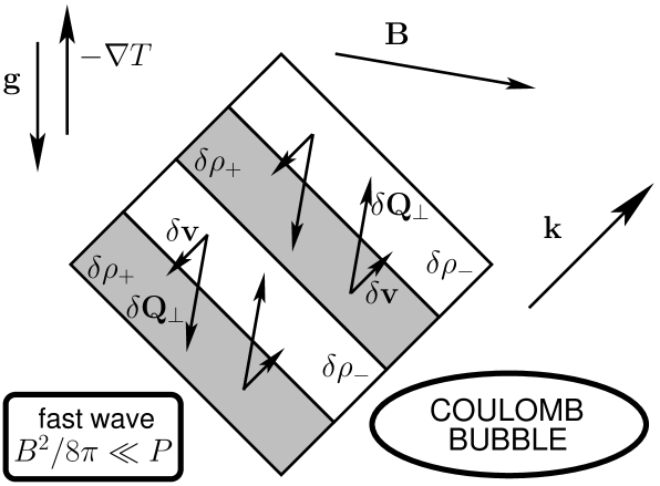
Figure 1: Geometry of the coulomb bubble instability. Here, the eigenfunction for a fast wave in a plasma with $B^{2}/8\pi/P\ll 1$ – nearly a standard hydrodynamic sound wave – is depicted. The velocity perturbation is perpendicular to surfaces of constant density and the perturbation of the perpendicular heat flux $\delta{\bf Q}_{\perp}$ lies along $\delta\hat{\bf b}$, the perturbation of field direction. Secular driving occurs because the wave in question possesses a finite projection along $\delta\hat{\bf b}$, which is $\perp$ to ${\bf B}$. Thus, both the fast and slow waves are driven by the coulomb bubble mechanism whether or not the plasma is weakly magnetized or not. The most strongly driven case corresponds to the example above i.e., a fast wave in a weakly magnetized plasma.

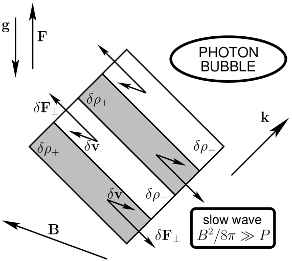
Figure 2: Geometry of the photon bubble instability. Both the fast and slow waves are driven by photon bubble driving. The most strongly driven case – represented above – is the slow wave in a strongly magnetized plasma.

5 An example: Interstellar Cosmic ray diffusion

We now understand the inner workings of the coulomb bubble driving mechanism and the equilibrium conditions in which such driving can operate. Now, we put our analysis to use with the example of interstellar cosmic ray diffusion.

5.1 Interstellar Cosmic Ray Diffusion and the “Two-Temperature” Approximation

Throughout the analysis above, we assert that the thermodynamics of the coulomb bubble instability is identical to that of the photon bubble instability. Though this statement is valid, it is not entirely complete. Blaes & Socrates (2003) considered the possibility of photon bubble driving in two distinct thermodynamic regimes. If the micro-physical processes responsible for absorption and emission act quickly enough to maintain thermal equilibrium between the fluctuating radiation and gaseous particle field, then the thermodynamics of photon driving and damping are encapsulated by a common temperature. In other words, absorption and emission occur rapidly in comparison to the dynamical time so that the radiation and gas temperature are locked to one another. So far, our analysis of the coulomb bubble has taken place under this “one-temperature” approximation.

If the particles endowed with a relatively high level of thermal mobility cannot come into close thermal contact with the bath of gaseous particles on a dynamical time, then the thermodynamics of radiative driving and damping is best described by a “two-temperature” approximation. An example of a system that is susceptible to photon bubble driving in the two-temperature limit is a magnetized envelope that is optically thick and whose only source of opacity is Thomson scattering.

Interstellar cosmic ray diffusion is another example of where the transfer of a radiative energy is best described in a two-temperature approximation. That is, the Galactic distribution of cosmic rays cannot come into local thermal equilibrium with the distribution of gaseous particles due to the absence of absorption and emission processes between the two species. Therefore, the thermodynamic state of the combined matter + cosmic ray fluid is constrained by the first law of thermodynamics for the matter gas given by eq. (A3) in addition to eq. (A4), the cosmic ray energy equation.

Though cosmic rays cannot directly exchange energy with the matter gas, they certainly can exchange momentum via resonant scattering with magnetic irregularities on the Larmor scale. For $\sim 1-10$ GeV cosmic ray protons – the energy range that is responsible for the majority of the Galactic cosmic ray pressure – the Larmor radius $r_{{}_{L}}$ is given by

$$r_{{}_{L}}\simeq 3\times 10^{12}\frac{\left(E_{{}_{\rm CR}}/{\rm GeV}\right)}{\left(B/\mu{\rm G}\right)}\,\,{\rm cm},$$ (62)

where $E_{{}_{\rm CR}}$ and $B$ is the cosmic ray energy and the large scale magnetic field strength, respectively. It follows that the length scale $r_{{}_{L}}$ of the resonant magnetic irregularities are much smaller than the inferred energy-weighted cosmic ray mean free path $\lambda_{{}_{\rm CR}}\sim 1$ pc (Ginzburg et al. 1980; Strong & Moskalenko 1998) and the scale height of the Galactic corona, which is $\sim$ a few kpc.

The cosmic ray pressure perturbation $\delta P_{{}_{\rm CR}}$ governs the exchange of momentum between fluctuations in the cosmic ray distribution and magnetofluid perturbations. The linearized Euler with the inclusion of the cosmic ray pressure force reads

$$-i\,\omega\rho\delta{\bf v}=-i\,{\bf k}\left[\delta P+\delta P_{{}_{\rm CR}}\right]+{\bf g}\,\delta\rho+\frac{i}{4\pi}\left({\bf k}\times\delta{\bf B}\right)\times{\bf B}=-i\,{\bf k}\left[\left(\frac{\partial P}{\partial\rho}\right)_{T}\delta\rho+\left(\frac{\partial P}{\partial T}\right)_{\rho}\delta T+\delta P_{{}_{\rm CR}}\right]+{\bf g}\,\delta\rho+\frac{i}{4\pi}\left({\bf k}\times\delta{\bf B}\right)\times{\bf B}.$$ (63)

If Galactic cosmic rays were a “normal” radiation species that could come into close thermal contact the matter through absorption and emission processes, then local thermal equilibrium between the radiation and matter distribution may occur and then both radiation and matter distributions may be characterized by a common temperature $T$. Upon perturbation, both radiation and particle species share the same temperature perturbation $\delta T$ as long as emission and absorption processes act quickly on dynamical timescales of interest (Blaes & Socrates 2003). For interstellar cosmic ray diffusion, the absence of any absorption and emission opacity necessarily implies that cosmic ray pressure perturbation $\delta P_{{}_{\rm CR}}$ and gas temperature perturbation $\delta T$ are separate and decoupled.

Below, we discuss the possibility that the diffusion of interstellar cosmic rays in the Galactic corona leads to a “two-temperature” version of the coulomb bubble instability.

5.2 Pressure Perturbation, Stability Criteria and Growth Rate

The diffusion of interstellar cosmic rays in the galactic disk and halo may lead to the two-temperature analogue of the photon bubble instability. In this case, cosmic rays, rather than photons, are responsible for the diffusive radiative transfer of energy. The action of cosmic rays scattering off of resonant magnetic irregularities leads to an “opacity” responsible for mediating momentum exchange between the radiation species and the gas. In the photon case, the relevant interaction is governed by Thomson scattering of photons with electrons. Rather than the radiation field diffusing along the gradient in the radiation pressure, cosmic rays diffuse along the projection of the cosmic ray pressure gradient that coincides with the equilibrium magnetic field. In what follows, we produce an abbreviated derivation of the growth rate $A_{0}$ for the coulomb bubble instability resulting from cosmic ray diffusion in the galactic corona.

The perturbation of the cosmic ray conductivity is given by

$$\frac{\delta\chi_{{}_{\rm CR}}}{\chi_{{}_{\rm CR}}}=-\frac{\delta\rho}{\rho}-\frac{\partial{\rm ln}\kappa_{{}_{\rm CR}}}{\partial{\rm ln}\rho}\frac{\delta\rho}{\rho}.$$ (64)

In Appendix A, we take note that $\partial{\rm ln}\kappa_{{}_{\rm CR}}/\partial{\rm ln}\rho\simeq-1$ for the Galactic halo. The implication being that $\delta\chi_{{}_{\rm CR}}\simeq 0$. However, we maintain the parameterization of $\delta\chi_{{}_{\rm CR}}$ given by eq. (64) in order to separate the effects of a “cosmic ray $\kappa$-mechanism” and coulomb bubbles.

The perturbation to the cosmic ray energy flux may be written as

$$\delta{\bf Q}_{{}_{\rm CR}}=-\chi_{{}_{\rm CR}}\left[-\frac{\delta\rho}{\rho}\hat{\bf b}\left(\hat{\bf b}\cdot\hbox{{\syvec\char 114\relax}}P_{{}_{\rm CR}}\right)-\frac{\partial{\rm ln}\kappa_{{}_{\rm CR}}}{\partial{\rm ln}\rho}\frac{\delta\rho}{\rho}\hat{\bf b}\left(\hat{\bf b}\cdot\hbox{{\syvec\char 114\relax}}P_{{}_{\rm CR}}\right)+\delta\hat{\bf b}\left(\hat{\bf b}\cdot\hbox{{\syvec\char 114\relax}}P_{{}_{\rm CR}}\right)+\hat{\bf b}\left(\delta\hat{\bf b}\cdot\hbox{{\syvec\char 114\relax}}P_{{}_{\rm CR}}\right)+i\,\hat{\bf b}\left({\bf k}\cdot\hat{\bf b}\right)\delta P_{{}_{\rm CR}}\right],$$ (65)

which then allows us to determine the cosmic ray pressure perturbation $\delta P_{{}_{\rm CR}}$ in terms of $\delta\rho$ and $\delta\hat{\bf b}$. The linear cosmic ray energy equation reads

$$-i\,\omega\delta P_{{}_{\rm CR}}+\frac{4}{3}i\,\omega P_{{}_{\rm CR}}\frac{\delta\rho}{\rho}-i\,\omega\hbox{{\gkvec\char 24\relax}}\cdot\left(\hbox{{\syvec\char 114\relax}}P_{{}_{\rm CR}}-\frac{4}{3}\frac{P_{{}_{\rm CR}}}{\rho}\hbox{{\syvec\char 114\relax}}\rho\right)=-i\,{\bf k}\cdot\delta{\bf Q}_{{}_{\rm CR}}.$$ (66)

The second term on the left hand side in above expression leads to diffusive Silk damping, while the third term is responsible for Brunt-Vaisalla oscillations. In §3.2 we took the high-$k$ limit of rapid diffusion of the first law of thermodynamics in order to isolate the temperature perturbation $\delta T$ in terms of the density and magnetic field unit vector perturbation $\delta\rho$ and $\delta\hat{\bf b}$, respectively. In order to study coulomb bubbles in the “two-temperature” approximation appropriate for cosmic ray diffusion, we likewise isolate the cosmic ray pressure perturbation $\delta P_{{}_{\rm CR}}$ in terms of $\delta\rho$ and $\delta\hat{\bf b}$ in the limit of rapid diffusion. By combining eqs. (65) and (66), the cosmic ray pressure perturbation becomes

$$\delta P_{{}_{\rm CR}} \simeq \frac{4}{3}\frac{\omega}{\omega_{\rm CR,diff}}P_{{}_{\rm CR}}\frac{\delta\rho}{\rho}-\frac{\omega}{\omega_{\rm CR,diff}}\hbox{{\gkvec\char 24\relax}}\cdot\left(\hbox{{\syvec\char 114\relax}}P_{{}_{\rm CR}}-\frac{4}{3}\frac{P_{{}_{\rm CR}}}{\rho}\hbox{{\syvec\char 114\relax}}\rho\right)$$ (67)

$$- \frac{\chi_{{}_{\rm CR}}}{\omega_{\rm CR,diff}}\left[-\frac{\delta\rho}{\rho}\left(1+\frac{\partial\,{\rm ln}\kappa_{{}_{\rm CR}}}{\partial{\rm ln}\rho}\right)\left({\bf k}\cdot\hat{\bf b}\right)\left(\hat{\bf b}\cdot\hbox{{\syvec\char 114\relax}}P_{{}_{\rm CR}}\right)+\left({\bf k}\cdot\delta\hat{\bf b}\right)\left(\hat{\bf b}\cdot\hbox{{\syvec\char 114\relax}}P_{{}_{\rm CR}}\right)+\left({\bf k}\cdot\hat{\bf b}\right)\left(\delta\hat{\bf b}\cdot\hbox{{\syvec\char 114\relax}}P_{{}_{\rm CR}}\right)\right],$$

where $\omega_{\rm CR,diff}=\omega+i\chi_{{}_{\rm CR}}\left({\bf k}\cdot\hat{\bf b}\right)^{2}$ is the characteristic cosmic ray diffusion frequency. In the limit of rapid diffusion, we take

$$|\omega_{\rm CR,diff}|\rightarrow\,\chi_{{}_{\rm CR}}\left({\bf k}\cdot\hat{\bf b}\right)^{2}\gg\omega.$$ (68)

Above, we take advantage of the fact that to leading order, the frequency of an acoustic oscillation is $\propto k$. With this, we have

$$\delta P_{{}_{\rm CR}} \simeq- \frac{4i}{3}\frac{\omega\,P_{{}_{\rm CR}}}{\chi_{{}_{\rm CR}}\left({\bf k}\cdot\hat{\bf b}\right)^{2}}\frac{\delta\rho}{\rho}+\frac{i}{\left({\bf k}\cdot\hat{\bf b}\right)^{2}}\left[-\frac{\delta\rho}{\rho}\left(1+\frac{\partial\,{\rm ln}\kappa_{{}_{\rm CR}}}{\partial{\rm ln}\rho}\right)\left({\bf k}\cdot\hat{\bf b}\right)\left(\hat{\bf b}\cdot\hbox{{\syvec\char 114\relax}}P_{{}_{\rm CR}}\right)+\left({\bf k}\cdot\delta\hat{\bf b}\right)\left(\hat{\bf b}\cdot\hbox{{\syvec\char 114\relax}}P_{{}_{\rm CR}}\right)+\left({\bf k}\cdot\hat{\bf b}\right)\left(\delta\hat{\bf b}\cdot\hbox{{\syvec\char 114\relax}}P_{{}_{\rm CR}}\right)\right].$$ (69)

The similarity is evident between $\delta P_{{}_{\rm CR}}$ above and the two-temperature radiation pressure perturbation $\delta P_{\rm rad}$ given by Blaes & Socrates (2003)

$$\delta P_{\rm rad}=\frac{1}{3}\,\delta E=-\frac{i}{k^{2}}\left[\frac{4E}{3}\frac{\omega}{\chi_{R}}\frac{\delta\rho}{\rho}+\frac{\delta\rho}{\rho}\left({\bf k}\cdot\hbox{{\syvec\char 114\relax}}P_{\rm rad}\right)\left(1+\frac{\partial\,{\rm ln\kappa_{F}}}{\partial\,{\rm ln}\rho}\right)\right],\,\,\,\,\,\,\,\,{\rm 2-TEMP\,\,\,\,RADIATIVE\,\,\,\,DIFFUSION}$$ (70)

where $\kappa_{F}$ is the flux mean opacity as defined in Blaes & Socrates (2003). Note that the Silk damping term of eq. (69) is smaller than the one found in eq. (70) by a factor of three, which results from our choice of parameterization of the cosmic ray diffusivity $\chi_{{}_{\rm CR}}$. We are now in the position to calculate the growth rate and stability criteria for the cosmic ray coulomb bubble instability. Following the analysis that led to eq. (44), the ratio of the asymptotic growth rate to acoustic oscillation frequency becomes

$$\frac{A_{0}}{\omega}\simeq\frac{1}{2}\frac{\frac{\Delta\rho}{\rho}\Delta P_{{}_{\rm CR}}}{\rho\,\delta{\bf v}\cdot\delta{\bf v}}.$$ (71)

Note that in the two-temperature case the velocity eigenvector oscillates at magnetoacoustic frequencies that are the solution to eq. (11). The quantitative difference is that the isothermal gas sound speed $c_{i}$ is replaced with the adiabatic gas sound speed $c_{s}$, since the gas neither generates nor loses any heat itself, the gas temperature perturbation then contributes to the acoustic response. In terms of its individual constituents, the growth rate may be written as

$$A_{0}\simeq\frac{{\tilde{\omega}}^{2}k^{2}}{2\omega\left[2\omega^{2}-k^{2}\left(c^{2}_{s}+v^{2}_{A}\right)\right]}\times\left[\frac{i}{\rho\chi_{{}_{\rm CR}}\left({\bf k}\cdot\hat{\bf b}\right)^{2}}\right]\Biggl{\{}-\frac{4}{3}\omega P_{{}_{\rm CR}}+\frac{2i\,{\tilde{\omega}}^{2}k^{2}}{\omega^{2}}\frac{\hbox{{\gkvec\char 24\relax}}\cdot\delta{\bf Q}_{{}_{\rm CR,}\perp}}{\left(\delta\rho/\rho\right)^{2}}+\frac{\partial\,{\rm ln}\kappa_{{}_{\rm CR}}}{\partial{\rm ln}\rho}\,\left({\bf k}\cdot{\bf Q}_{{}_{\rm CR}}\right)\Biggl{\}}.$$ (72)

The form of $A_{0}$ not only serves as an asymptotic growth rate, but as a stability criteria as well. The first term in the $\{\}$ leads to Silk damping, the second term results in the coulomb bubble instability and the last term is responsible for a $\kappa_{{}_{\rm CR}}-$mechanism. The quantity $\delta{\bf Q}_{{}_{\rm CR},\perp}=\left({\bf 1}-\hat{\bf b}\hat{\bf b}\right)\cdot\delta{\bf Q}_{{}_{\rm CR}}$ is the cosmic ray flux perturbation that is $\perp$ to the equilibrium field ${\bf B}$ (and equilibrium cosmic ray flux ${\bf Q}_{{}_{\rm CR}}$). It follows that the geometry and mechanics of the two-temperature cosmic ray coulomb bubble instability is identical to the one-temperature coulomb bubble instability.

In terms of the wave vector and specified equilibrium parameters, the asymptotic growth rate becomes

$$A_{0}\simeq\frac{{\tilde{\omega}}^{2}k^{2}}{2\omega\left[2\omega^{2}-k^{2}\left(c^{2}_{s}+v^{2}_{A}\right)\right]}\times\left[\frac{i}{\rho\chi_{{}_{\rm CR}}\left({\bf k}\cdot\hat{\bf b}\right)^{2}}\right]\Biggl{\{}-\frac{4}{3}\omega P_{{}_{\rm CR}}+\frac{2\omega^{2}}{{\tilde{\omega}}^{2}}\left({\bf k}\cdot{\bf Q}_{{}_{\rm CR}}\right)\left[1-\frac{\left({\bf k}\cdot\hat{\bf b}\right)^{2}}{k^{2}}\right]+\frac{\partial\,{\rm ln}\kappa_{{}_{\rm CR}}}{\partial{\rm ln}\rho}\left({\bf k}\cdot{\bf Q}_{{}_{\rm CR}}\right)\Biggl{\}}.$$ (73)

5.3 Marginal Stability of the Galactic Corona

As stated in Appendix A, Galactic cosmic rays almost uniformly fill a halo (or corona) with a characteristic thickness $\sim$ a few kpc. Over these scales, the coronal gas is hot ($T\sim 10^{6}$ K) and tenuous $n\sim 10^{-3}\,{\rm cm^{-3}}\equiv n_{3}$ and the corresponding adiabatic gas sound speed $c_{s}\sim 10^{7}T^{1/2}_{6}{\rm cm/s}$, where $T_{6}$ is temperature in units of $10^{6}$ K. For our stability analysis, we take the halo equilibrium field to be uniform with a characteristic value of $B\sim 1\mu{\rm G}\equiv B_{{\mu{\rm G}}}$, corresponding to an Alfvén velocity $v_{A}\lesssim 10^{7}B_{{\mu{\rm G}}}\,n^{-1/2}_{3}{\rm cm/s}$, somewhat less than the adiabatic sound speed $c_{s}$. The average local pressure for gas and cosmic ray protons in the interstellar medium is roughly $\sim 1{\rm eV/cm^{3}}\sim 10^{-12}\,{\rm erg/cm^{3}}$. Due to the large $\sim$ a few kpc scale height for the cosmic rays, this value of pressure also corresponds to the coronal value of the cosmic ray pressure $P_{{}_{\rm CR}}\sim 1{\rm eV/cm^{3}}$. Compare this with the value of the coronal gas pressure $P\sim 10^{-1}\,n_{3}\,T_{6}\,{\rm eV/cm^{3}}$. Thus, the ratio of cosmic ray to gas pressure is $P_{{}_{\rm CR}}/P\sim 10$ in the kpc-scale galactic corona, a somewhat surprising value. In short, the Galactic corona is a cosmic ray pressure supported atmosphere.

In the diffusion approximation, the cosmic ray flux $Q_{{}_{\rm CR}}$ for a plane-parallel geometry satisfies the relation

$$\frac{\tau_{{}_{\rm CR}}}{c}Q_{{}_{\rm CR}}\sim P_{{}_{\rm CR}}.$$ (74)

For a disk-like geometry the corresponding cosmic ray luminosity $L_{{}_{\rm CR}}$ is roughly

$$L_{{}_{\rm CR}}\sim 5\times 10^{40}P_{1}\,\tau^{-1}_{3.5}\,R^{2}_{10}\,{\rm erg\,s^{-1}}$$ (75)

where $\tau_{3.5}$, $P_{1}$ and $R_{10}$ is the cosmic ray optical depth in units of $10^{3.5}$, halo cosmic ray pressure in units of $1\,{\rm eV/cm^{3}}$ and characteristic cylindrical emitting radius in units of 10 kpc, respectively. We now have the necessary ingredients to determine whether or not the kpc-scale galactic corona is over-stable to either the coulomb bubble instability or the $\kappa$-mechanism. When calculating the growth or damping rates resulting from cosmic ray diffusion, we assume that the equilibrium field is relatively uniform over a wavelength and that it does not contribute to hydrostatic balance as well.

In §4.4 we made note of the fact that the coulomb bubble instability is most strongly driven for waves that closely resemble simple propagating hydrodynamic sound waves i.e., the fast wave in the limit where $c^{2}_{s}\gg v^{2}_{A}$. In this case, the instability condition for cosmic ray coulomb bubble driving from eq. (73) is approximately

$$Q_{{}_{\rm CR}} > P_{{}_{\rm CR}}\,c_{s}\longrightarrow\frac{c}{\tau_{{}_{\rm CR}}}>c_{s}.$$ (76)

In the above expression we ignore geometrical and other factors of order unity. Interestingly, the quantity $c/\tau_{{}_{\rm CR}}$, which represents the diffusive drift velocity $v_{\rm D}$ over the coronal scale height, is close in value to the adiabatic gas sound speed i.e., $v_{D}\sim\tau^{-1}_{3.5}\,10^{7}{\rm cm/s}\sim c_{s}\sim 10^{7}T^{1/2}_{6}{\rm cm/s}$. Altogether the condition for instability is satisfied as long as $T^{1/2}_{6}\tau_{3.5}<1$. The growth rate $\Gamma_{{}_{\rm FAST}}$ for the fast wave coulomb bubble instability in the $c^{2}_{s}\gg v^{2}_{A}$ limit is given by

$$\Gamma_{{}_{\rm FAST}}\sim\frac{g}{c_{s}}\sim\frac{c_{{}_{\rm CR}}}{c_{s}}\frac{g}{c_{{}_{\rm CR}}}\sim\sqrt{\frac{P_{{}_{\rm CR}}}{P}}\frac{V_{\rm circ}}{H_{c}}\sim 3\times 10^{-7}\,\sqrt{\frac{P_{{}_{\rm CR}}/P}{10}}\,V_{300}\,H^{-1}_{3}\,{\rm yrs^{-1}},$$ (77)

where $V_{300}$ is the circular velocity $V_{\rm circ}$ in units of $300\,{\rm km/s}$ and $H_{3}$ is the coronal scale height in units of 3 kpc. The growth rate $\Gamma_{{}_{\rm FAST}}$ is dynamical and indicates that the fast wave coulomb bubble instability can transform a low amplitude propagating fast wave, with phase velocity equal to $c_{s}$, into a large amplitude sonic disturbance over a relatively few wave crossing times.

5.4 Coulomb Bubbles vs. the $\kappa$-Mechanism

The approximate stability criteria and growth rate for a $\kappa_{{}_{\rm CR}}-$ mechanism is identical to that of the cosmic ray coulomb bubble instability in the corona of the Galaxy. Fast waves in the weakly magnetized limit, with $\omega\simeq k\,c_{s}$, are the strongest growing excitations for both cases. However, eq. (73) informs us that upward propagating fast waves are driven by the coulomb bubble instability while downward propagating fast waves are driven by the $\kappa_{{}_{\rm CR}}-$mechanism, for $\partial{\rm ln}\kappa_{{}_{\rm CR}}/\partial{\rm ln}\rho\simeq-1$.

At the base of the corona, the Galactic disk is highly inhomogeneous and turbulent. The turbulence in the interstellar medium primarily results from explosive phenomena – expanding HII regions, line-driven stellar winds and core-collapse SNe – that originates, in some way, from massive stars. There are $\sim 10^{4}$ O stars in the Milky Way within a galactocentric radius of $\sim 10$ kpc. Therefore, the characteristic separation between luminous massive stars $\sim 100$ pc is roughly the scale $l_{T}$ at which the interstellar turbulence is stirred.

With respect to the Galactic corona, the dense multiphase disk serves as a source of acoustic radiation that can then be amplified in the corona by either the cosmic ray coulomb bubble instability or the $\kappa_{{}_{\rm CR}}-$mechanism. The direction of propagation for the seed $k^{-1}\sim l_{T}\sim 100$ pc-scale acoustic fluctuations is primarily upwards with respect to gravity in the Galactic corona since the dense disk lies at its base. It follows that the cosmic ray coulomb bubbles are the the relevant mechanism that amplifies propagating acoustic perturbations arising from the Galactic disk rather than a $\kappa_{\rm{}_{CR}}-$mechanism.

6 Summary

We have identified a new acoustic over-stability, which we refer to as the “coulomb bubble instability,” that is driven by the rapid diffusion of energy along magnetic field lines. From a linear instability analysis, we calculate the condition for over-stability and the growth rate of the coulomb bubble instability. Driving occurs when the ratio of heat flux to entropy is relatively large for the equilibrium, implying that the heat flux is the physical quantity that provides the free energy required for the over-stability. The coulomb bubble instability may be thought of as a standard magnetoacoustic wave that is driven by $\delta{\bf Q}_{\perp}=\left({\bf 1}-\hat{\bf b}\hat{\bf b}\right)\cdot\delta{\bf Q}$, the linear perturbation of the coulomb heat flux that is $\perp$ to the direction of the equilibrium field $\hat{\bf b}={\bf B}/B$ (and thus ${\bf Q}=-\chi\hat{\bf b}\hat{\bf b}\cdot\hbox{{\syvec\char 114\relax}}T$ as well). The growth rate of the coulomb instability is dynamical for the fast wave in the $B^{2}/8\pi\ll P$ limit – roughly a standard hydrodynamic sound wave – such that the growth time is roughly the sound crossing time over a gas pressure scale height.

The properties of the coulomb bubble instability are, at the same time, strikingly similar and starkly different from the photon bubble instability. The thermodynamic properties of both instabilities are identical in that the rapid diffusion of thermal energy in a stratified flow is needed in order for driving to occur. The work done upon the fluid by the driving force for both instabilities is proportional to the product of the Lagrangian density and temperature perturbation $\Delta\rho\,\Delta T$. Furthermore, and like the photon bubble instability, both the fast and the slow wave are susceptible to over-stability from the coulomb bubble mechanism irrespective of whether or not the background flow is strongly magnetized.

Work is done upon the wave by the coulomb bubble linear driving force provided by $\delta{\bf Q}_{\perp}$, the component of the heat flux perturbation that is $\perp\hat{\bf b}$. The fast and slow magnetosonic waves are polarized along both the wavevector ${\bf k}$ due to compression, and along the direction of the magnetic field ${\bf b}$, which results from magnetic tension. In general, $\delta{\bf Q}_{\perp}$ has some finite projection that is coincident with the wavevector ${\bf k}$ – as long as ${\bf k}\nparallel\hat{\bf b}$ – which allows driving to occur, since all compressible fluctuations exhibit motion that is in part $\parallel{\bf k}$. On the other hand, the photon bubble linear driving force originates from $\delta{\bf F}_{\perp}=\left({\bf 1}-{\bf k}{\bf k}/k^{2}\right)\cdot\delta{\bf F}$, the component of the radiative heat flux perturbation that is $\perp{\bf k}$. Since the magnetic tension force partially polarizes magnetosonic waves along $\hat{\bf b}$, the radiative driving force due to $\delta{\bf F}_{\perp}$ is coincident with the motion of the fluid, which then allows the radiation field to perform work upon the fluid. Clearly, in describing the geometry of the driving mechanisms for the coulomb bubble and photon bubble instability, the vectors ${\bf k}$ and $\hat{\bf b}$ are interchanged with one another in every possible way. From this, we conclude that the coulomb bubble instability is the mirror opposite of the photon bubble instability.

Both the fast and slow magnetosonic waves are driven over-stable by the coulomb bubble mechanism. The fast mode in the weakly magnetized limit is the most strongly driven case, with a growth rate $\sim g/c_{g}$, where $c_{g}$ is the gas sound speed. If the equilibria in question resembles a stellar envelope, then both the coulomb bubble instability and Balbus’ magnetothermal instability possess comparable growth rates. However, if the particles responsible for the transfer of thermal energy along field lines (e.g. cosmic rays) are not the particles responsible for providing the acoustic response (the gas), then the growth rate of the coulomb bubble instability is larger than the magnetothermal instability by a factor that is $\sim c_{{}_{\rm CR}}/c_{i}\sim\sqrt{P_{{}_{\rm CR}}/P}$, for the case of cosmic ray diffusion in the Galactic halo.

The coulomb bubble instability may thrive in a wide variety of astrophysical environments. For example, it is possible that coulomb bubbles play an important role in the modifying the thermal transport properties of the envelopes of magnetized neutron stars, central cooling flows of galaxy clusters and interstellar cosmic ray diffusion. In the latter case, we show that the kpc-scale galactic corona is a setting in which a cosmic ray coulomb bubble instability possibly operates. For commonly accepted values of cosmic ray and gas pressure, cosmic ray luminosity and coronal gas temperature, the Galactic corona is in a state of marginal stability with respect to a cosmic ray coulomb bubble instability. The implication being that cosmic ray coulomb bubbles self-regulates the interstellar cosmic ray pressure on Galactic scales.

6.1 What Is To Be Done?

Our local linear analysis is only the first step in realizing whether or not the coulomb bubble instability has practical applications. At this simple exploratory level, we only examine local propagating WKB waves at linear order. The next step is to perform a global linear analysis, where a linear mode is really the combination of an upward and downward propagating wave, whose properties are further augmented by the specified boundary conditions. Of course, linear theory can only tell us whether an instability exists. A MHD computer algorithm that incorporates the effects of rapid anisotropic diffusion in a stratified atmosphere is most likely the correct tool in fully studying the non-linear outcome of the coulomb bubble instability.

Appendix A An envelope partially supported by Cosmic Rays

In order to describe the physics of cosmic ray diffusion in a stratified atmosphere, we amend the conservation laws and equilibrium conditions of §2. Conservation of momentum now reads

$$\rho\left(\frac{\partial{\bf v}}{\partial t}+{\bf v}\cdot\hbox{{\syvec\char 114\relax}}{\bf v}\right)=-\hbox{{\syvec\char 114\relax}}\left(P+P_{{}_{\rm CR}}\right)+\rho\,{\bf g}+\frac{1}{4\pi}\left(\hbox{{\syvec\char 114\relax}}\times{\bf B}\right)\times{\bf B},$$ (A1)

where $P_{{}_{\rm CR}}$ is the cosmic ray pressure – dominated by $\sim 1-10$ GeV cosmic ray protons in the interstellar medium. The first law of thermodynamics for the gas

$$\rho T\left(\frac{\partial s}{\partial t}+{\bf v}\cdot\hbox{{\syvec\char 114\relax}}s\right)=0$$ (A2)

now implies that fluid-matter perturbations are adiabatic. Evolution of the cosmic ray pressure $P_{{}_{\rm CR}}$ is further constrained by a cosmic ray-energy equation

$$\frac{\partial P_{{}_{\rm CR}}}{\partial t}+{\bf v}\cdot\hbox{{\syvec\char 114\relax}}P_{{}_{\rm CR}}+\frac{4}{3}P_{{}_{\rm CR}}\hbox{{\syvec\char 114\relax}}\cdot{\bf v}=-\hbox{{\syvec\char 114\relax}}\cdot{\bf Q}_{{}_{\rm CR}},$$ (A3)

where we assume that adiabatic index of the cosmic rays is that of a relativistic ideal gas i.e., $\gamma_{{}_{\rm CR}}=4/3$. The cosmic ray energy flux ${\bf Q}_{{}_{\rm CR}}$ is given by

$${\bf Q}_{{}_{\rm CR}}=-\chi_{{}_{\rm CR}}\hat{\bf b}\hat{\bf b}\cdot\hbox{{\syvec\char 114\relax}}P_{{}_{\rm CR}},$$ (A4)

which is similar in form to the coulombic heat flux given by eq. (4).

The cosmic ray conductivity $\chi_{{}_{\rm CR}}$ deserves discussion as its prescription for the Galaxy differs from the prescription for thermal conductivity $\chi$ described in §3.1. Measurements of the cosmic ray transport in the Milky Way indicate a cosmic ray mean free path $\lambda_{{}_{\rm CR}}\sim 1$pc. Interestingly, models of Galactic cosmic ray transport are consistent with $\lambda_{{}_{\rm CR}}$ roughly being a constant over a “halo” scale height of $\sim$ a few kpc. It follows that the cosmic ray “opacity” $\kappa_{{}_{\rm CR}}$ must vary inversely with density i.e., $\kappa_{{}_{\rm CR}}\propto\rho^{-1}$. The immediate suggestion is that a “cosmic ray $\kappa$-mechanism” may operate in the galactic halo since $\partial{\rm ln}\kappa_{{}_{\rm CR}}/\partial{\rm ln}\rho\neq 0$ and is given by

$$\frac{\partial\,{\rm ln}\kappa_{{}_{\rm CR}}}{\partial\,{\rm ln}\rho}\simeq-1.$$ (A5)

Finally, the only other basic assumption that differs from those given in §2 involves hydrostatic balance

$$-\frac{1}{\rho}\hbox{{\syvec\char 114\relax}}\left(P+P_{{}_{\rm CR}}\right)={\bf g}.$$ (A6)

That is, partial support of the atmosphere is given by an equilibrium cosmic ray pressure gradient.

References

• Arons (1992) Arons, J. 1992, ApJ, 388, 561
• Baker&Kippenhanh (1962) Baker, N. & Kippenhahn, R. 1962, ZA, 54, 114
• Balbus (2001) Balbus, S.A. 2001, ApJ, 62, 909
• BS (01) Blaes, O.M. & Socrates, A. 2001, ApJ, 553, 987
• BS03 (2003) Blaes, O.M. & Socrates, A. 2003, ApJ, 596, 509 BS03
• Chan (2006) Chandran, B. & Dennis, T.J. 2006, ApJ, 642, 140
• Gammie (1998) Gammie, C.F. 1998 MNRAS, 297, 929
• Ginzburg (1980) Ginzburg, V.L., Khazan, Ia. M., & Ptuskin, V.S. 1980, Ap&SS, 68, 295
• Parrish (2005) Parrish, I.J. & Stone, J.M. 2005, ApJ, 633, 334
• Socrates (2005) Socrates, A., Blaes, O., Hungerford, A. & Fryer, C.L. 2005, ApJ, 632, 531
• Silk (1968) Silk, J. 1968, ApJ, 151, 459
• Turner (2005) Turner, N. J., Blaes, O., Socrates, A., Begelman, M. C., & Davis, S. W. 2005, ApJ, 624, 267
• Weinberg (1971) Weinberg, S. 1971, ApJ, 168, 175