Spitzer Limits On Dust Emission and Optical Gas Absorption Variability Around Nearby Stars with Edge-On Circumstellar Disk Signatures

Abstract

We present Spitzer Space Telescope infrared spectroscopic and photometric observations and McDonald Observatory Smith Telescope and Anglo-Australian Telescope high spectral resolution optical observations of 4 nearby stars with variable or anomalous optical absorption, likely caused by circumstellar material. The optical observations of Ca II and Na I cover a 2.8 year baseline, and extend the long term monitoring of these systems by previous researchers. In addition, mini-surveys of the local interstellar medium (LISM) around our primary targets provide a reconstruction of the intervening LISM along the line of sight. We confirm that the anomalous absorption detected toward $\alpha$ Oph is not due to circumstellar material, but to a small filamentary cloud $<$14.3 pc from the Sun. The three other primary targets, $\beta$ Car, HD85905, and HR10 show both short and long term variability, and little of the observed absorption can be attributed to the LISM along the line of sight. The Spitzer Space Telescope photometry and spectroscopy did not detect infrared excesses. We fit the maximum hypothetical infrared excess that is consistent with observed upper limits. We are able to place upper limits on any possible fractional infrared luminosity, which range from $L_{IR}/L_{\star}<2$–$5\times 10^{-6}$, for our three disk stars. These fractional luminosities are significantly less than that found toward $\beta$ Pic, but comparable to other nearby debris disks. No stable gas absorption component centered at the radial velocity of the star is detected for any of our targets, consistent with no infrared excess detections. Based on simple assumptions of the variable gas absorption component, we estimate limits on the circumstellar gas mass causing the variable absorption, which range from 0.4–20 $\times 10^{-8}M_{\oplus}$. These multiwavelength observations place strong limits on any possible circumstellar dust, while confirming variable circumstellar gas absorption, and therefore are interesting targets to explore the origins and evolution of variable circumstellar gas.

1 Introduction

The presence of circumstellar gas around mature stars presents an interesting diagnostic of the formation and evolution of stars and their immediate environments. A collection of “shell” stars, including stars that exhibit strong and sharp absorption features (e.g., in Ca II) and sometimes hydrogen emission lines (i.e., Be stars), include many examples of stars in which gas from the stellar atmosphere is deposited in the circumstellar environment via winds (Slettebak, 1988; Porter & Rivinius, 2003). Slettebak (1975) identified $\beta$ Pic as an object that displayed strong and sharp absorption in Ca II that they postulated might be circumstellar. Indeed, observations with the Infrared Astronomical Satellite (IRAS) led to the discovery of dust disks around $\beta$ Pic ($L_{\rm dust}/L_{\star}\sim 3\times 10^{-3}$; Backman & Paresce 1993), and other nearby stars, including Vega, $\epsilon$ Eri, and $\alpha$ PsA (Aumann, 1985). The gas and dust in the circumstellar environment of $\beta$ Pic have been shown to be distributed in an edge-on disk by Brandeker et al. (2004) and Smith & Terrile (1984), respectively. Although $\beta$ Pic shares some diagnostic characteristics of “shell” stars, it has become clear that its observed gas and dust are the secondary products left from the final stages of stellar formation, which has resulted in a debris disk. Therefore, two possible mechanisms exist for depositing substantial amounts of circumstellar gas, one is associated with debris disks and stellar formation and the other with shell stars and stellar winds.

In the process of studying the properties of the circumstellar gas in the dusty edge-on disk surrounding $\beta$ Pic, high resolution optical (Ca II and Na I) spectra showed night-to-night absorption line variability, evidence of a variable circumstellar gas component located close to the star (Hobbs et al., 1985; Vidal-Madjar et al., 1986). Of the four major dust disks discovered by IRAS, (i.e., $\beta$ Pic, Vega, $\alpha$ PsA, and $\epsilon$ Eri), only $\beta$ Pic shows Ca II absorption line variability. $\beta$ Pic is also the only one to have an edge-on orientation, which allows for a detectable optical depth along the line of sight through the midplane of the circumstellar disk, and may explain why it is the only one of the four major dust disks to show gas phase absorption. Indeed, if the three-dimensional density profile of Na I in the disk around $\beta$ Pic, derived by Brandeker et al. (2004), is observed from inclinations consistent with the other three major dust disks, the resulting observable Na I column density falls well below the threshold of detectability.

The formation of stars and planets appears to necessarily include the construction (and subsequent dispersal) of disks comprised of gas and dust. Therefore, it is likely that every star has experienced a transitory phase in which the secondary gas and dust products of stellar and planetary formation lead to a debris disk. Understanding the process of disk formation, evolution, and dissipation is critical to placing known stellar and planetary systems, including our own, into context. Observations with the Spitzer Space Telescope (Spitzer) are finding much fainter debris disks than observed toward $\beta$ Pic, around much older stars. Spitzer has detected dusty material in stars similar in age to the Sun, with $L_{\rm dust}/L_{\star}\sim 3\times 10^{-6}$ (e.g., Chen et al., 2005; Silverstone et al., 2006; Beichman et al., 2006; Chen et al., 2006), whereas our solar system zodiacal dust emits $\sim$10${}^{-7}L_{\odot}$. In particular, Su et al. (2006) find that such disks are quite common, with $\sim$1/3rd of a sample of $\sim$160 A stars showing infrared (IR) excesses due to a debris disk.

If we use $\beta$ Pic as a prototypical debris disk, the structure of dust and gas in the circumstellar disk can be characterized by three distinct components. (1) The large-scale bulk dust disk, which causes an IR excess (e.g., Aumann, 1985) and scattered light emission (e.g., Smith & Terrile, 1984). (2) The large-scale bulk gas disk, which causes a stable gas absorption feature (Brandeker et al., 2004). (3) The variable gas component of the disk, which is located very close to the star and causes gas absorption line variability over short (e.g., night-to-night) timescales (e.g., Petterson & Tobin, 1999). For reviews of the various properties of all the components of the $\beta$ Pic debris disk, see Zuckerman (2001), Lagrange, Backman, & Artymowicz (2000), and Vidal-Madjar, Lecavelier des Etangs, & Ferlet (1998).

The source of the variable gas absorption component of the $\beta$ Pic disk has received particular attention. Long Ca II monitoring campaigns of $\beta$ Pic (e.g., Petterson & Tobin, 1999), support the theory that the short-term spectral variability is due to gas clouds caused by evaporating, star-grazing, kilometer-sized, cometary-like bodies, simply referred to as, Falling Evaporating Bodies (FEB’s; Thébault & Beust, 2001; Beust, 1994). The dynamics and frequency of these events, potentially originating from a mean-motion resonance with a giant planet, can constrain the structure of the disk and even the geometry of a young planetary system (Beust & Morbidelli, 2000).

No detailed study, comparable to the work on $\beta$ Pic, on the variability of gas absorption in an edge-on disk toward a shell or Be star has been made to date. Despite the fact that gas may be deposited irregularly in the circumstellar environment of rapidly rotating, early type stars via weak stellar winds, like a scaled down version of the disks that form around Be stars. Abt, Tan, & Zhou (1997) describe three epochs of observations toward shell stars taken over a 20 year baseline, and note the long term variations in the strength of the gas absorption. In order to understand the origins and structure of circumstellar gas around mature stars it is critical to increase the sample of known edge-on circumstellar gas absorption systems and measure as comprehensively as possible the properties of gas and any dust in the circumstellar environment.

Researchers have tried to find other circumstellar gas disks or $\beta$ Pic-like systems (i.e., edge-on debris disks) through IR excesses from IRAS (Cheng et al., 1992) and Ca II variability (Lagrange-Henri et al. 1990b; Holweger, Hempel, & Kamp 1999). To date, several other main sequence edge-on circumstellar disk systems have been studied, including $\beta$ Car (Lagrange-Henri et al., 1990b; Hempel & Schmitt, 2003), HD85905 (Welsh et al., 1998), HR10 (Lagrange-Henri et al., 1990a; Welsh et al., 1998), AU Mic (Kalas, Liu, & Matthews 2004; Roberge et al. 2005), and HD32297 (Schneider, Silverstone, & Hines 2005, Redfield 2007).

We selected three of the Ca II and Na I variable objects (i.e., $\beta$ Car, HD85905, and HR10) together with $\alpha$ Oph, which has an anomalously high absorption signature in these ions (Crawford, 2001), to study any gas and dust in their circumstellar environments. We monitored their optical absorption properties to probe the stable and variable components of the gas disk (see Section 3.1). Observations of their IR emission were also made in order to look for any excess due to a dusty debris disk (see Section 4).

In addition, we conducted mini-surveys of a handful of stars in close angular proximity to our program stars to look for absorption due to intervening interstellar gas. Measuring the interstellar medium (ISM) along the line of sight and in the locality directly surrounding a circumstellar disk candidate, is critical to reconstructing the distribution of possible “contaminating” ISM absorption (Crawford, 2001; Redfield, 2007). In particular, the Sun resides in a large scale structure known as the Local Bubble, whose boundary at $\sim$100 pc is defined by a significant quantity of interstellar material (Lallement et al., 2003). These mini-surveys allow us to differentiate between a stable circumstellar absorption component and an interstellar absorption feature (see Section 3.2).

Our program stars are all rapidly rotating, and therefore likely close to edge-on (i.e., their $v\sin i$ places them on the high velocity tail of the distribution of predicted equatorial rotational velocities, and therefore $\sin i\sim 1$; Abt & Morrell, 1995). They are relatively mature systems, with ages of several hundreds of millions of years, based on isochronal fitting (see Section 4). Although they are older than $\beta$ Pic, which is $\sim$12 Myr, they are comparable in age to other stars with debris disks, such as Vega and $\alpha$ PsA (Barrado y Navascues, 1998), as well as our solar system during the Late Heavy Bombardment (Gomes et al., 2005). Therefore, with evidence that these systems have an edge-on orientation, and ages consistent with the final stages of planetary system formation, our program stars are inviting targets with which to makes observations of secondary gas and dust products that may still reside in their circumstellar environments.

2 Observations

Our sample was determined with the intent to investigate $\beta$ Pic like systems, that is, edge-on circumstellar disks that are in the evolutionary transition period of clearing their dusty debris disks. These edge-on transitional systems provide an opportunity to probe properties of both the dust, via IR spectral energy distributions (SEDs), and gas, through atomic absorption lines. We selected 4 systems, see Table 1, that were suspected of having gas disks, from absorption line variability on timescales of days to years, or anomalous Ca II absorption features that have been difficult to attribute solely to local interstellar medium (LISM) absorption. Three of the four targets (HR10, HD85905, and $\beta$ Car) show Ca II and/or Na I absorption variability (Lagrange-Henri et al., 1990a; Welsh et al., 1998; Hempel & Schmitt, 2003). The fourth target, $\alpha$ Oph, has an anomalously large Ca II column density compared to observations of other nearby stars (Redfield & Linsky, 2002). Crawford (2001) observed 8 angularly close stars and detected Ca II absorption in 2 stars which were significantly more distant (120–211 pc) than $\alpha$ Oph (14.3 pc), leaving open the possibility that the absorption toward $\alpha$ Oph is circumstellar in origin. None of our targets had significant IR excess detections with IRAS, although these observations were not sensitive enough to reach the stellar photospheres.

Our observational strategy included (1) continued high resolution optical spectroscopy of our primary targets to monitor the short term variability of atomic absorption lines, Section 3.1, (2) observations of several stars close in angle and distance to our primary targets in order to reconstruct the LISM absorption profile along the line of sight, and to be able to distinguish between interstellar absorption and a stable circumstellar feature, Section 3.2, and (3) Spitzer observations of the IR SED to search for excess emission from dust and bulk gas emission lines in a circumstellar disk, Sections 4 and 5.

2.1 Optical Spectroscopy

High resolution optical spectra were obtained using the Coudé Spectrometers on the 2.7m Harlan J. Smith Telescope at McDonald Observatory and the Ultra High Resolution Facility (UHRF) on the 3.9m Anglo-Australian Telescope (AAT) at the Anglo-Australian Observatory (AAO). Observations began in October 2003 and continued until July 2006, a temporal baseline of 2.8 years. The observational parameters for our primary targets are given in Table 2 and stars proximate to our primary targets in Table 3. During this interval, repeated observations of our primary targets monitored absorption variability on timescales from days to years, and observations of close neighbors surveyed the spatial and radial variations in the interstellar medium around our primary targets. Two atomic doublets were monitored: Ca II H and K (3968.4673 and 3933.6614 Å, respectively) and Na I D₁ and D₂ (5895.9242 and 5889.9510 Å, respectively). These are among the strongest transitions in the optical wavelength band, appropriate for observing absorption toward nearby stars (Redfield, 2006).

The McDonald spectra were obtained with a range of resolving powers. High resolution spectra ($R\,\equiv\,\lambda/\Delta\lambda\,\sim\,$400,000) were obtained using the CS12 double-pass configuration (Tull, 1972). The detector was TK4, a 1024 $\times$ 1024 Tektronix CCD chip, with 24 $\mu$m pixels. The resolution was confirmed using the HeNe laser line at 6328 Å, at $R\,=\,$520,000. Only a single order falls on the detector, and therefore the spectral range in this configuration is very small, $\sim$1.4 Å near Ca II at 3934 Å, and $\sim$2.0 Å near Na I at 5896 Å, too small to observe both transitions in the doublet simultaneously. We also utilized the 2dcoudé Spectrograph (Tull et al., 1995) in both the CS21 configuration ($R\,\sim\,$240,000) and the CS23 configuration ($R\,\sim\,$60,000). The detector was TK3, a 2048 $\times$ 2048 Tektronix CCD chip, with 24 $\mu$m pixels. The resolutions were confirmed using the HeNe laser line at 6328 Å, at $R\,=\,$210,000 for CS21 and $R\,=\,$70,000 for CS23. The spectral range for CS21 near the Ca II doublet (3934 and 3968 Å) is $\sim$570 Å with $\sim$30 Å gaps between orders, and near the Na I doublet (5890 and 5896 Å) is $\sim$2800 Å with $\sim$130 Å gaps between orders. In either configuration both lines of the doublet (of either Ca II or Na I) can be observed simultaneously.

The AAO spectra were obtained with the highest resolving power available ($R\,\sim\,$940,000), using the UHRF spectrograph (Diego et al., 1995). The detector was EEV2, a 2048 $\times$ 4096 CCD chip, with 15 $\mu$m pixels. The resolution was confirmed using the HeNe laser line at 6328 Å, at $R\,=\,$1,090,000. Only a single order falls on the detector, but due to the large chip size, the spectral range is $\sim$4.8 Å near Ca II at 3934 Å, and $\sim$7.2 Å near Na I at 5896 Å, although again, too small to easily observe both transitions in either the Ca II or Na I doublets simultaneously. By utilizing an image slicer (Diego, 1993), the throughput is significantly better than single slit high resolution spectrographs.

The data were reduced using Image Reduction and Analysis Facility (IRAF; Tody, 1993) and Interactive Data Language (IDL) routines to subtract the bias, flat field the images, remove scattered light and cosmic ray contamination, extract the echelle orders, calibrate the wavelength solution, and convert to heliocentric velocities. Wavelength calibration images were taken using a Th-Ar hollow cathode before and after each scientific target.

The extracted one-dimensional spectra were then normalized using fits of low order polynomials to regions of the continuum free of interstellar and telluric absorption lines. Numerous water vapor lines are commonly present in spectra around the Na I doublet. Although the telluric H₂O lines are relatively weak, they need to be modeled and removed from the spectrum, in order to measure an accurate Na I absorption profile, particularly for observations toward nearby stars which may be expected to exhibit weak interstellar (or circumstellar) absorption. The traditional telluric subtraction technique of observing a nearby, rapidly rotating, early type star at a similar airmass in order to divide out an empirically derived telluric spectrum is not feasible for observations of our nearby targets. It is precisely our primary targets, which are nearby, rapidly rotating, early type stars and likely candidates themselves to be used as a telluric standard, that we want to scrutinize for interstellar or circumstellar absorption. Instead, we use a forward modeling technique demonstrated by Lallement et al. (1993) to remove telluric line contamination in the vicinity of the Na I D lines. We use a relatively simple model of terrestrial atmospheric transmission (AT - Atmospheric Transmission program, from Airhead Software, Boulder, CO) developed by Erich Grossman to fit and remove the telluric water vapor lines. Observing both transitions of the Na I doublet is an important confirmation that the telluric subtraction is successful. With two independent measurements of Na I absorption at the same projected velocity, it is easy to identify contaminating telluric absorption. No telluric features fall near the Ca II H & K lines.

Atmospheric sodium absorption was occasionally detected, particularly in high signal-to-noise ($S/N$) spectra. This absorption is easily identified at the Doppler shift of the projected velocity of the Earth’s atmosphere in the heliocentric rest frame. This projected velocity is given in Table 2 for all Na I observations. For the vast majority of Na I observations, the location of an atmospheric absorption line is well separated from any astrophysical absorption features.

2.2 Infrared

The IR observations were obtained with Spitzer (Werner et al., 2004), from 2004 September through 2005 September. Table 4 lists dates and astronomical observation request (AOR) numbers. Near-IR photometry from 3.6 to 8.0 $\mu$m was obtained with the Infrared Array Camera (IRAC; Fazio et al., 2004), and mid- to far-IR photometry was obtained with the Multiband Imaging Photometer for Spitzer (MIPS; Rieke et al., 2004). Moderate resolution spectroscopy ($R\,\approx 160$–600) in the 10–37 $\mu$m range was obtained with Short-High (SH) and and Long-High (LH) modules of the Infrared Spectrograph (IRS; Houck et al., 2004), while low resolution ($R\approx 15$–25) spectroscopy in the 55–95 $\mu$m region was obtained with the SED mode of MIPS.

2.2.1 Spitzer Photometry

The IRAC and MIPS 24 $\mu$m data were processed using the the c2d mosaicking/source extraction software, c2dphot, (Harvey et al., 2004) which is based on the mosaicking program, Astronomical Point Source Extraction (APEX), developed by the Spitzer Science Center (SSC) and the source extractor Dophot (Schechter, Mateo, & Saha, 1993). While the photometric measurement uncertainties are small ($\sim$5$\%$ and $\sim$9$\%$) for IRAC and MIPS 24 $\mu$m sources with good $S/N$, the absolute calibration uncertainty is estimated to be 10$\%$ (Evans et al. 2006).

We used the Mosaicking and Point Source Extraction (MOPEX) software package version 030106(Makovoz & Khan, 2005), to create 70 and 160 $\mu$m mosaics starting from the basic calibrated data (BCD) processed by the Spitzer Science Center (SSC) through the S14.4 pipeline (Spitzer Science Center, 2006). We used the median-filtered BCDs provided by the SSC, which are optimized for photometry of point sources. Only two of our sources, $\alpha$ Oph and $\beta$ Car, are clearly detected at 70 $\mu$m. We obtained 70 $\mu$m fluxes and uncertainties for $\alpha$ Oph and $\beta$ Car using MOPEX point-source fitting from half-pixel (i.e., 4$\arcsec$) re-sampled mosiacs. We obtained 70 $\mu$m upper limits for HR 10 and HD 85905 through aperture photometry from mosaics re-sampled at the original pixel scale. We use an aperture with a radius of 16$\arcsec$ and a sky annulus with an inner and an outer radius of 48 and 80$\arcsec$, respectively. Based on high $S/N$ 70 $\mu$m point sources identified in the BCD mosaics of the Spitzer c2d Legacy project (program identification (PID) = 173), we derived a multiplicative aperture correction ($AC$) of 1.6. Thus, we compute the observed 70 $\mu$m flux, $F_{70}=FA_{70}\times AC$, where $FA_{70}$ is the flux within the aperture minus the contribution from the sky. We estimate a 1$\sigma$ photometric uncertainty, $\sigma=AC\times RMS_{\rm sky}\times n^{1/2}$, where $RMS_{\rm sky}$ is the root mean square (RMS) of the pixels in the sky annulus, and $n$ is the number of pixels in our aperture. An absolute calibration uncertainty, estimated to be 20$\%$ (Evans et al. 2006), is added in quadrature to the photometric uncertainties for MIPS 70 $\mu$m and 160 $\mu$m. $\alpha$ Oph and $\beta$ Car are detected with $S/N\sim 30$, while HD85905 and HR10 are very close to the 70 $\mu$m detection limit (e.g., $F_{70}\sim 3\times\sigma$). We note that the absolute calibration uncertainty is estimated at the 20$\%$ level for 70 $\mu$m observations (Spitzer Science Center, 2006), and becomes the dominant source of error for moderate and high $S/N$ observations.

None of our four sources are detected at 160 $\mu$m. The MIPS 160 $\mu$m channel has a short-wavelength filter leak in which stray light in the wavelength range of 1–1.6 $\mu$m produces a ghost image offset $\sim$40 arcsecs from the true 160 $\mu$m image. The leak is only detectable above the confusion limit for sources brighter than $J\sim 5.5$ (Spitzer Science Center, 2006). Given the brightness of $\alpha$ Oph and $\beta$ Car ($J=1.75$ and 1.55, respectively), their MIPS 160 $\mu$m images are severely affected by this leak. For our two fainter targets, HR10 and HD85905 ($J=5.85$ and 6.05, respectively), the 160 $\mu$m signal produced by the near-IR leak should be just below the 160 $\mu$m confusion limit expected from extragalactic sources (Dole et al., 2004). In this case, we use an aperture 32$\arcsec$ in radius and a sky annulus with an inner and an outer radius of 40 and 80$\arcsec$, respectively. We adopt an aperture correction of 2.0, appropriate for the size of our aperture and sky annulus. Similar to the 70 $\mu$m upper limits, we calculate the 1$\sigma$ uncertainty, $\sigma=AC\times RMS_{\rm sky}\times n^{1/2}$, from mosaics re-sampled at the original pixel scale. The 160 $\mu$m flux at the position of all four sources is affected by the short-wavelength leak. Therefore, we adopt a conservative 3$\sigma$ upper limit by adding 3$\sigma$ to the flux measured at the source position.

2.2.2 Spitzer Spectroscopy

The IRS spectra were extracted via the c2d Interactive Analysis (c2dia) reduction environment (F. Lahuis et al. 2006, in preparation). Prior to extraction, the dither positions are combined, reducing noise and adding to spectral stability. The spectra are extracted using an optimal point spread function (PSF) extraction, in which an analytical cross dispersion PSF, defined from high $S/N$ observations of a calibrator, is fit to the collapsed order data by varying the offset for the trace and width of the source profile. The observed signal is assumed to be that of a point source plus a uniform zero level (representing extended/sky emission). The amplitude of the zero level is determined via the profile fitting method and used to make sky corrections. The optimal PSF extraction uses a fit to the good pixels only, therefore direct bad/hot pixel corrections are not required. The final spectra are defringed using the IRSFRINGE package developed by the c2d team.

MIPS SED spectra were calibrated and coadded using MOPEX. The spectra were then extracted from the coadded images via standard methods using the IRAF apall tool within the National Optical Astronomy Observatories (NOAO) TWODSPEC package. Wavelength calibration and aperture corrections were performed post extraction by using the “MIPS70 SED sample calibration” file provided by the SSC with the MOPEX package (version 030106).

Two of the four sources (HR10 and HD85905) were not detected in the IRS LH module, and 3$\sigma$ upper limits are used together with our photometric measurements to constrain the estimates of the excess emission (Section 4). Additionally, no gas-phase atomic or molecular lines or solid-state silicate or polycyclic aromatic hydrocarbon (PAH) bands were detected in the Spitzer spectra (Section 5).

3 Detections and Constraints on Variable Circumstellar Gas

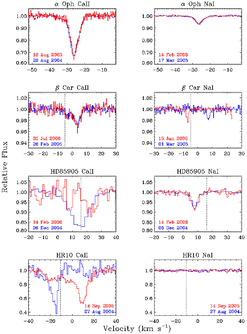
Figure 1: Examples of typical Ca II and Na I spectra taken at two different epochs for all 4 primary targets. The vertical dotted line indicates the stellar radial velocity. Both ions are shown on the same scale, and it is clear that the Ca II absorption is much stronger than Na I in all cases. Temporal variability is immediately obvious in Ca II observations of HD85905 and HR10, and in Na I of $\beta$ Car. These examples include spectra taken at various spectral resolution from both the McDonald Observatory H.J. Smith Telescope and the AAT. Note the success of telluric subtraction in the Na I spectra.

Gas phase absorption due to Ca II and Na I gas phase atoms was monitored in spectra of all four targets. Table 2 details the observational parameters. All targets were observed over short ($\sim$few nights) and long ($\sim$few months) timescales, spanning 2.75 years. Examples of observed spectra are shown in Figure 1. Two epochs are shown for each star to emphasize any variability and demonstrate the use of different spectrographs and spectral resolutions. The $\alpha$ Oph absorption, which shows no evidence for variability, exemplifies the consistency in data collection and reduction over 7 months while using two different instruments (CS21 and UHRF). HD85905 and HR10 show clear evidence for variability over these two epochs, while only the Na I profiles of $\beta$ Car varied significantly over the two epochs shown. The temporal variability of the entire dataset will be discussed in detail in Section 3.1.

Figure 1 also shows quite clearly that the observed Na I column density is significantly lower relative to the observed Ca II absorption. In fact, we detect only very weak ISM or circumstellar Na I absorption toward HR10, despite it being our most distant sightline and therefore likely to traverse significant ISM material. It does show quite strong circumstellar absorption in Ca II. The constant Na I absorption in HD85905, despite the variability in Ca II presumably from a circumstellar gas disk, may be a signature of the intervening ISM along this line of sight, rather than the circumstellar disk. The “contamination” of interstellar absorption on our observations of gas in circumstellar disks will be discussed in Section 3.2 where spectra of stars in close angular proximity to our targets are presented.

3.1 Temporal Variability

Figure 1 shows that variability is detected in 3 of our 4 targets. In order to characterize the absorption profile we use the apparent optical depth (AOD) method (Savage & Sembach, 1991) to calculate the observed column density in each velocity bin. An alternative characterization would be to model the absorption profile with a series of Gaussian components, as is often done in high resolution ISM absorption line analysis (e.g., Welty, Hobbs, & Kulkarni, 1994; Crawford & Dunkin, 1995), and is particularly straightforward in observations of the simple absorption profiles seen toward nearby stars, where only 1–3 components are detected (Redfield & Linsky, 2001). Component fitting has also been used successfully to characterize variable absorption due to circumstellar material (e.g., Welsh et al., 1998). However, the ability to attach physical properties with the parameters used to fit the series of Gaussian absorption profiles is highly sensitive to the physical distinctiveness in projected velocity of the absorbing medium and the resolving power of the spectrograph. In other words, a one-to-one correspondence must exist between an absorbing structure and an observed absorption component in order to make meaningful physical measurements. For example, physical properties (e.g., temperature) can be derived from a Gaussian fit to the line width for ISM absorption toward the nearest stars, since 1 absorption component is observed and the path length is so short that only 1 absorbing cloud is traversed (Redfield & Linsky, 2004). However, the circumstellar environment giving rise to the variable absorption profiles is likely too complicated (e.g., coincident projected velocities from different absorbing sites) to allow for a straightforward correspondence with a series of Gaussian components. Therefore, we employ the AOD technique to characterize the observed absorption.

The AOD method is well described in Savage & Sembach (1991), and has been used extensively to model absorption profiles (e.g., Jenkins & Tripp, 2001; Roberge et al., 2002). In brief, the apparent optical depth ($\tau_{a}$) in velocity ($v$) space is

$$\tau_{a}(v)=\ln\frac{I_{0}(v)}{I_{\rm obs}(v)}\;,$$ (1)

where $I_{\rm obs}(v)$ is the observed spectrum, and $I_{0}(v)$ is the continuum spectrum expected if no interstellar or circumstellar absorption were present. In a normalized spectrum, as shown in Figure 1, the stellar background intensities have already been divided out, and $I_{0}(v)\,=\,1$. Equation 1 does not describe the true optical depth, since the instrumental line spread function (LSF) is folded into our observed spectrum ($I_{\rm obs}(v)$).

The column density ($N_{a}$) in each velocity bin can be calculated from the apparent optical depth,

$$N_{a}(v)=\frac{m_{e}c}{\pi e^{2}}\frac{\tau_{a}(v)}{f\lambda}\;\;[{\rm cm}^{-2}]\;,$$ (2)

where $f$ is the oscillator strength of the transition, and $\lambda$ is the wavelength of the velocity bin. The total column density can be calculated by integrating $N_{a}(v)$ over the velocity range of interest. Equation 2 provides accurate total column densities provided the absorption is unsaturated. Since both Ca II and Na I are doublets, we have two independent measurements of the absorbed column density in transitions with different oscillator strengths. A comparison of $N_{a}(v)$ for the two transitions in each doublet confirms the absorption is unsaturated. A final $N_{a}(v)$ is calculated for each ion by taking the weighted mean of $N_{a}(v)$ calculated for each transition. By utilizing the information from both transitions in the doublet, the impact of numerous systematic uncertainties (e.g., continuum placement, telluric line subtraction, wavelength calibration) is greatly reduced.

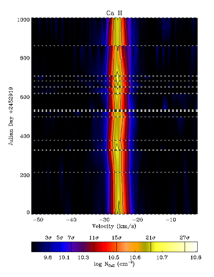
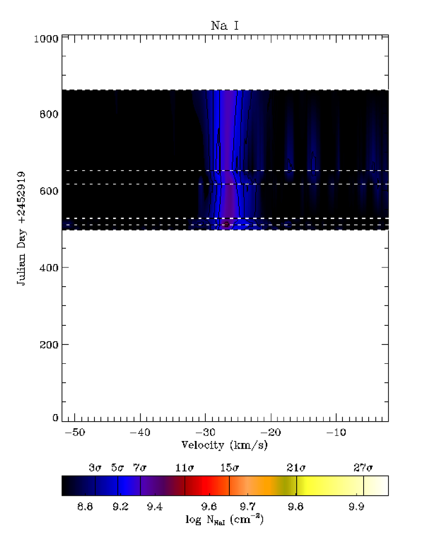
Figure 2: Three dimensional data cubes of the observed column density, signified by the colored contours, in Ca II (left) and Na I (right), toward $\alpha$ Oph. The data are shown as a function of projected velocity and date of observation. Although the colored contours are displayed as continuous through time, observations are sporadic and indicated by the horizontal hatched lines. A simple interpolation between observations is used to create the continuous data cube. The color-coding is normalized in $S/N$ between Ca II and Na I, so that it is clear that the Ca II absorption is much stronger compared to Na I. Little, if any, variation is detected in the absorption toward $\alpha$ Oph.

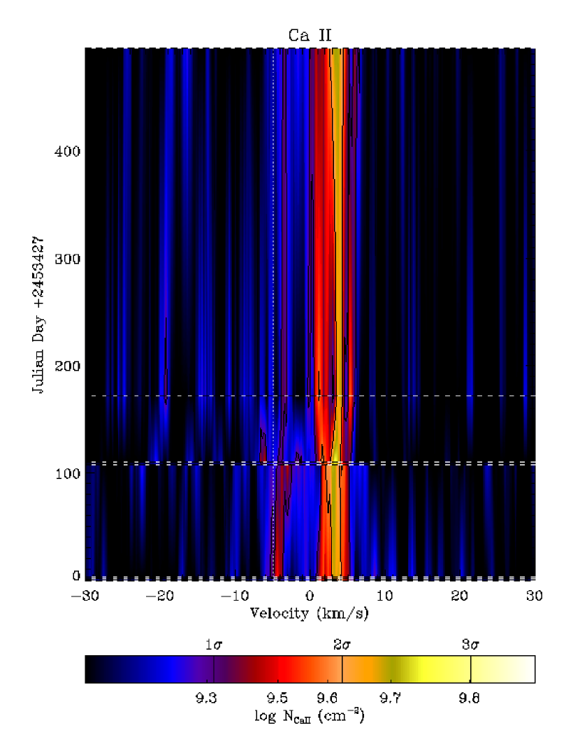
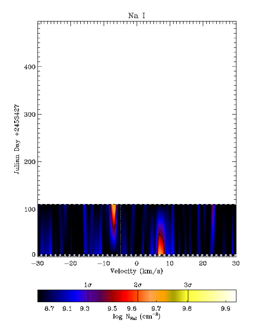
Figure 3: Same as Figure 2 for absorption toward $\beta$ Car. The vertical dotted line indicates the stellar radial velocity. Some slight variation is detected in Ca II, and clear temporal variability is seen in Na I.

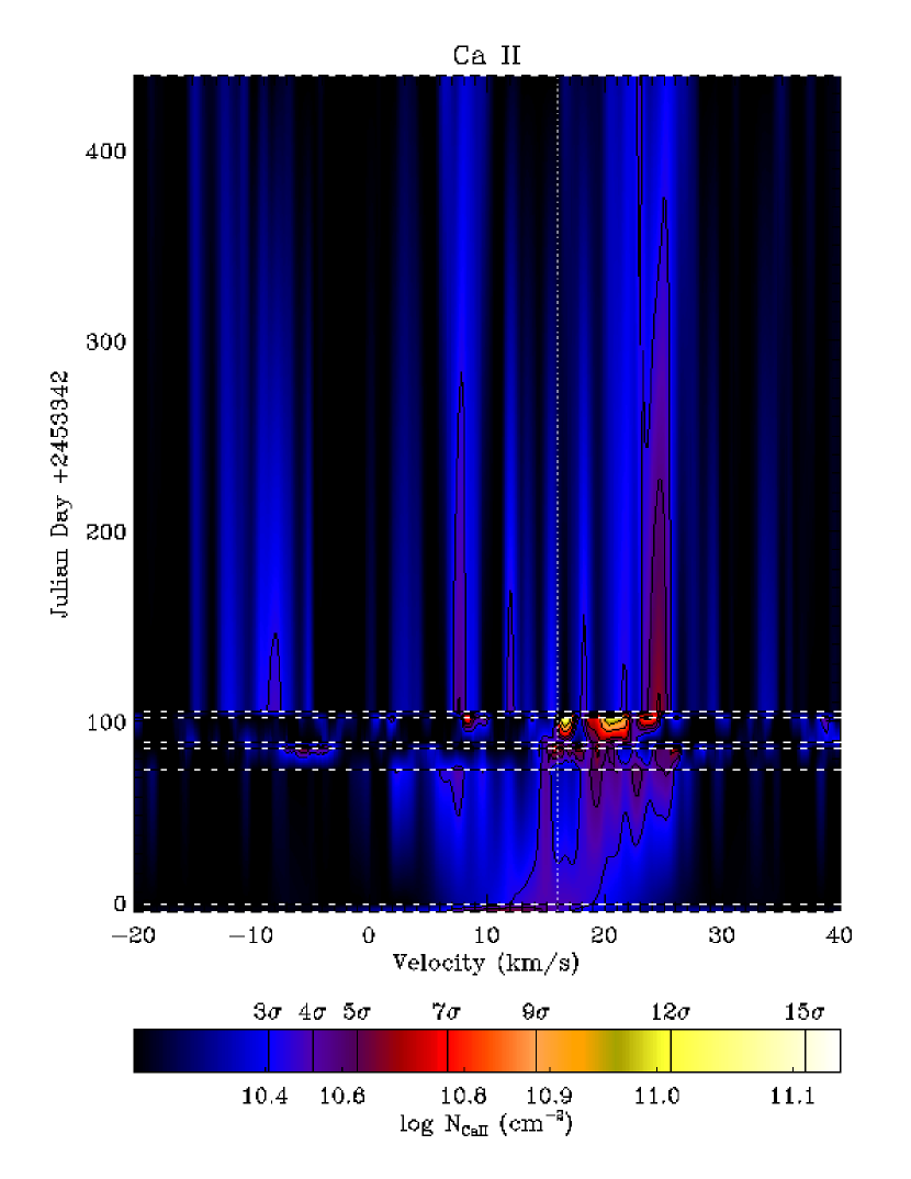
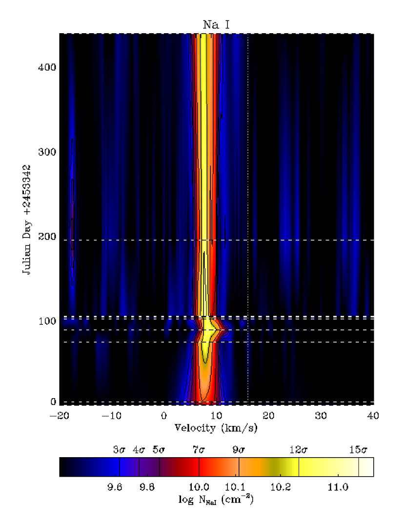
Figure 4: Same as Figure 2 for absorption toward HD85905. The vertical dotted line indicates the stellar radial velocity. Temporal variation is detected in Ca II, while a relatively constant feature, likely interstellar, is seen in Na I.

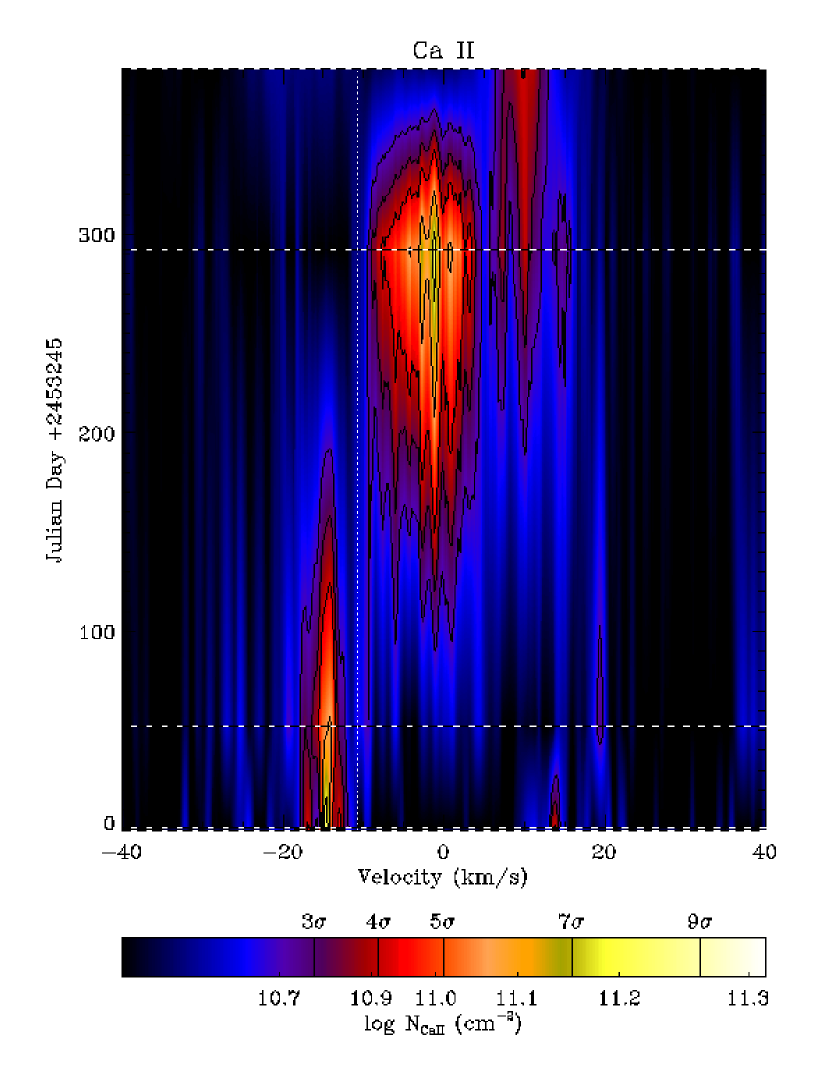
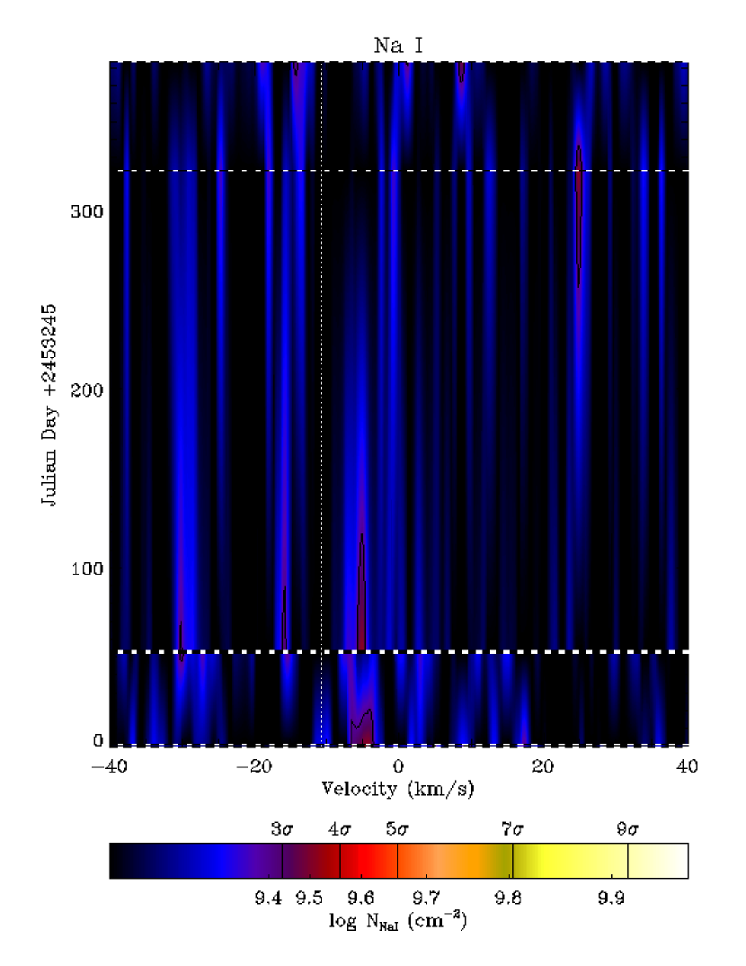
Figure 5: Same as Figure 2 for absorption toward HR10. The vertical dotted line indicates the stellar radial velocity. Strong temporal variation is detected in Ca II, while only very weak absorption is detected in Na I.

Another challenge of evaluating the temporal variability of absorption profiles is amalgamating the data of a long monitoring campaign. Even comparing the spectra of only two epochs, as in Figure 1, can be confusing. Comparing spectra directly in such a way for as many as 26 epochs is impractical. Each observation results in an array of measurements of the column density as a function of velocity (derived from the normalized flux as a function of wavelength as described above). Therefore, we have a sporadic data cube. Figures 2–5 are three-dimensional contour plots of observed column density as a function of velocity as a function of time, for all 4 targets. It is important to note that the observations are sporadic and not continuous in time. The date of each observation is highlighted with a hatched line, and the contours between epochs are simple interpolations between the two observations. Occasionally closely spaced observations, (e.g., $<$1 week apart), cannot be distinguished in Figures 2–5 and can be associated with an apparent discontinuity. It is likely that subtle changes, such as in Ca II toward $\alpha$ Oph in Figure 2 or Na I toward HD85905 in Figure 4 are caused by systematic effects, whereas obvious circumstellar variability is seen for example in Ca II toward HR10 in Figure 5. The short and long-term temporal variability is discussed in detail below. For each target, the color coding is normalized between Ca II and Na I such that column density measurements of comparable $S/N$ are displayed with the same color. For example, the normalization of $S/N$ makes it clear in Figure 2, that the Na I feature is clearly weaker when compared to the strong Ca II absorption.

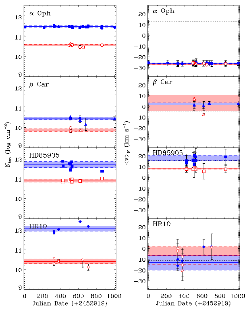
Figure 6: Total column density (left) and column density weighted velocity (right) measurements of absorption toward our primary targets as a function of time. The filled symbols indicate Ca II observations, while open symbols indicate Na I. The error bars are the weighted average variance, and in the case of $\langle v\rangle_{N}$ indicate the range of observed velocities rather than the error in measuring the central velocity of absorption. The shaded regions (blue corresponds to Ca II, and red with Na I) indicate the weighted mean and weighted average variance of the absorption detected in the primary target, presented in Figure 6. The horizontal dotted line in the right panels indicates the radial velocity of the star. Three of our four targets show some signs of temporal variation. Only the spectra toward $\alpha$ Oph shows no hint of variation. The data is also presented in Table 5.

Some basic attributes of the temporal variability data cubes are summarized in Figure 6. For each observation, the total column density, $N_{\rm tot}=\int^{v_{2}}_{v_{1}}N_{a}(v)dv$, and the column density weighted velocity, $\langle v\rangle_{N}=\sum\limits_{i=v_{1}}^{v_{2}}v_{i}N_{i}/N_{\rm tot}$ are plotted, where $v_{1}$ and $v_{2}$ indicate the range of velocities over which the absorption is detected. The error bars on the total column density are often smaller than the symbol size. The “error bars” shown in the column density weighted velocity are the weighted average variance (Bevington & Robinson, 1992). Therefore, the “errors” shown for $\langle v\rangle_{N}$ are not the error in determining the central velocity of absorption, which for these high resolution spectra range from 0.1–2.0 km s^-1, but the range of velocities with significant absorption. For example, in the case of the Ca II spectra shown for HR10 in Figure 1, for the 27 Aug 2004 spectrum, $\langle v\rangle_{\rm CaII}=-15.9$ km s^-1, and a weighted average variance of only 2.6 km s^-1. The fact that the weighted average variance is relatively small matches the fact that the absorption profile spans a narrow range of velocities around –16 km s^-1. The 14 Sep 2005 spectrum, on the other hand, shows a narrow absorption component around 9 km s^-1, as well as significant weak absorption that ranges from –25 to 5 km s^-1. Since the absorption covers a wide range of velocities and is asymmetric, $\langle v\rangle_{\rm CaII}$ is not centered exactly on the narrow component but at 1.8 km s^-1, and the weighted average variance is relatively large, 12.1 km s^-1, since absorption is detected over a wide range of velocities. The total column density and the column density weighted velocity of each observation is listed in Table 5.

Figures 1–6 indicate that no temporal variability is detected toward $\alpha$ Oph in either observed ion. The Ca II absorption observed toward $\beta$ Car is relatively constant, but variation is seen in Na I. HD85905 shows some Ca II variability, but relatively constant Na I absorption, likely dominated by absorption from interstellar material in the Local Bubble shell, which will be discussed in Section 3.2. HR10 shows dramatic Ca II temporal variability, but little to no absorption, interstellar or circumstellar, is detected in Na I.

3.1.1 Search for Short Term Variability

Short-term variability, on time scales of nights or hours, is detected in two of our targets: HD85905 and HR10. Night-to-night measurements are provided in Table 5. Such short temporal variations have been detected in $\beta$ Pic (Ferlet, Vidal-Madjar, & Hobbs, 1987) and in these two stars by (Welsh et al., 1998). Column density variations from night-to-night can reach factors $\geq$2, while shifts in velocity of $\geq$10 km s^-1 are detected. However, the magnitude and frequency of short variations in our targets remains lower than detected toward the prototypical edge-on debris disk, $\beta$ Pic, where single feature night-to-night variations in column density can exceed a factor of 10, and 20 km s^-1 in radial velocity (Petterson & Tobin, 1999).

3.1.2 Comparison of Contemporaneous Ca II and Na I Observations

Contemporaneous observations of both Ca II and Na I absorption toward circumstellar disk stars, even $\beta$ Pic, are relatively rare. There is a strong preference to observe the Ca II lines rather than the Na I lines, because Na I is significantly less abundant (see Section 3.3) and it is difficult to model and remove the telluric lines that populate the spectral region near Na I. Welsh et al. (1997, 1998) monitor both Ca II and Na I for several edge-on circumstellar disks, including $\beta$ Pic, HD85905, and HR10. In the case of $\beta$ Pic, only the strong component at the rest frame of the star is detected in both ions, while no time variable absorbers have ever been detected in Na I. Toward HD85905 and HR10, Welsh et al. (1998) detect absorption in both ions, often with little one-to-one correspondence in the velocity of the absorption between Ca II and Na I. Although, it is important to note that the ions were not observed during the same night, but on adjacent nights.

Although rarely simultaneous, many of our observations of Ca II and Na I were taken one after the other during the same night. The nightly measurements, given in Table 5, can be used to compare such contemporaneous absorption measurements of Ca II and Na I. Both ions show the same absorption feature toward $\alpha$ Oph, although, as discussed in Section 3.2.1, this feature is not circumstellar in origin, but a result of interstellar absorption along the line of sight. Toward $\beta$ Car, the Ca II and Na I absorption features do not match in velocity. The Ca II is relatively constant and distinct from the narrow and weak Na I absorption. It is possible that we are sampling two different collections of material, and the relatively constant Ca II feature is part of the extended disk, while Na I is found in the variable gas component. Toward HD85905, a comparison between contemporaneous Ca II and Na I observations shows little correspondence, although there is the possibility that the Na I absorption is due to the interstellar medium, as discussed in Section 3.2.2. The contemporaneous observations toward HR10 are typically consistent between Ca II and Na I, such as the 2005 September and 2004 October observations. However, the 2004 August observations of Ca II and Na I are not consistent in velocity, similar to the earlier observations by Welsh et al. (1998), where Ca II and Na I absorption features differ between adjacent nights.

3.1.3 Distribution of Red- vs. Blue-shifted Features

The velocity distribution of the variable circumstellar absorption features relative to the rest frame of the host star is an important constraint on the dynamics of the absorbing gas. Toward $\beta$ Pic, the majority of variable absorption features are redshifted relative to the rest frame of the star, although blueshifted absorption is not particularly rare (Crawford, Beust, & Lagrange, 1998; Petterson & Tobin, 1999). Although we do not have the temporal sampling of some of the monitoring campaigns of $\beta$ Pic (e.g., Petterson & Tobin, 1999), we are able to quantify the frequency of redshifted versus blueshifted absorption features. Using the radial velocities listed in Table 1, we calculated the fraction of the total absorption that was redshifted relative to the radial velocity of the star, i.e., $f_{\rm red}=\int^{\infty}_{v_{\rm R}}N(v)/\int^{\infty}_{-\infty}N(v)$. For $\beta$ Car, $f_{\rm red}($Ca II$)$ ranged from 80–100%, while $f_{\rm red}($Na I$)$ ranged from 4–100%, indicating the stability of the Ca II feature in contrast to Na I. Toward HD85905, $f_{\rm red}($Ca II$)$ ranged from 25–79%, while $f_{\rm red}($Na I$)$ ranged from 0–2%, although as discussed in Section 3.2.2, there is a possibility that the Na I feature is caused by the interstellar medium. Toward HR10, $f_{\rm red}($Ca II$)$ ranged from 0–98%, while $f_{\rm red}($Na I$)$ ranged from 44–100%. In contrast to $\beta$ Pic, the velocity of variable absorption toward our three circumstellar disk stars did not have a distribution dominated by redshifted radial velocities.

3.1.4 Search for Very Long Term Variability

The primary targets were selected based on previous evidence of anomalous or variable gas phase atomic absorption. This work builds on that of previous studies, and presents an opportunity to search for very long term variability, on the timescale of decades. Table 5 details the absorption characteristics observed during the monitoring campaign presented in this work, as well as past measurements by other researchers. We have limited the literature search to relatively high spectral resolution observations ($R\geq 60$,000).

Our measurements of Ca II and Na I toward $\alpha$ Oph are constant and consistent with past observations. Some of the total column density measurements are slightly lower than the present values (e.g., Hempel & Schmitt, 2003). However, the central velocity has remained steady throughout at approximately $-25.8$ km s^-1, and systematic errors are expected due to the different instruments and analysis techniques employed. For example, a new analysis by Crawford (2001) of identical data from Crawford & Dunkin (1995) led to a slight increase in column density, from $\log N_{\rm CaII}=11.38$ to 11.54, which matches the mean value of the present monitoring campaign, which is $\log N_{\rm CaII}=11.53$.

The variation we see in the total column density of Ca II toward $\beta$ Car, $\log N_{\rm CaII}=10.18$–$10.56$, is similar to the variation detected by Hempel & Schmitt (2003), $\log N_{\rm CaII}=10.14$–$10.50$. The previous nondetection of Na I toward $\beta$ Car of $\log N_{\rm NaI}<10.23$ by Welsh et al. (1994) is consistent with the relatively weak absorption features that are detected in the present campaign, which range from $\log N_{\rm NaI}=9.87$–$10.15$. The radial velocity of the Na I features varied by 14.4 km s^-1 over the two epochs, from $v_{\rm NaI}=-7.1$ to $+7.3$ km s^-1.

Variation in velocity ($v_{\rm CaII}=12.4$ to $20.2$ km s^-1) and column density ($\log N_{\rm CaII}=11.39$–$11.91$) is detected in Ca II absorption toward HD85905, just as it has been in a previous campaigns ($v_{\rm CaII}=-11.5$ to $+7.0$ km s^-1, $\log N_{\rm CaII}=11.97$–$12.24$; Welsh et al., 1998). We do not see as dramatic velocity shifts, nor quite as large total column densities, but the magnitude of variability in column density is comparable. We see a relatively stable Na I component in velocity ($v_{\rm NaI}\sim 8.2$ km s^-1), which shows subtle column density variations ($\log N_{\rm NaI}=10.82$–$11.02$). This is similar to the 1997 November observations by Welsh et al. (1994), $v_{\rm NaI}=9.2$ and $\log N_{\rm NaI}=11.22$. However, over a temporal baseline of 1.2 years, we see no dramatic variation, while in two epochs spaced by $\sim$10 months, Welsh et al. (1994) observed a dramatic shift in velocity to $v_{\rm NaI}=-10.8$ and a subtle weakening in column density, $\log N_{\rm NaI}=11.02$.

The dramatic Ca II absorption variability toward HR10 ($v_{\rm CaII}=-15.9$ to $+1.8$ km s^-1, $\log N_{\rm CaII}=11.87$–$12.44$) is similar to variations seen in previous observations in velocity ($v_{\rm CaII}=-6.8$ to $+6.1$ km s^-1) and total column densities ($\log N_{\rm CaII}=11.87$–$12.62$). The Na I columns ($\log N_{\rm NaI}=10.13$–$10.59$) are significantly smaller for this campaign than observed by Welsh et al. (1998), $\log N_{\rm NaI}=11.09$–$11.49$. The upper limits by Hobbs (1986) ($\log N_{\rm NaI}<11.0$) and Lagrange-Henri et al. (1990b) ($\log N_{\rm NaI}<10.5$)are consistent with the present campaign’s low column densities, and indicates that the high column density absorption epoch detected by Welsh et al. (1998) was short-lived.

3.2 Comparison With Proximate Targets

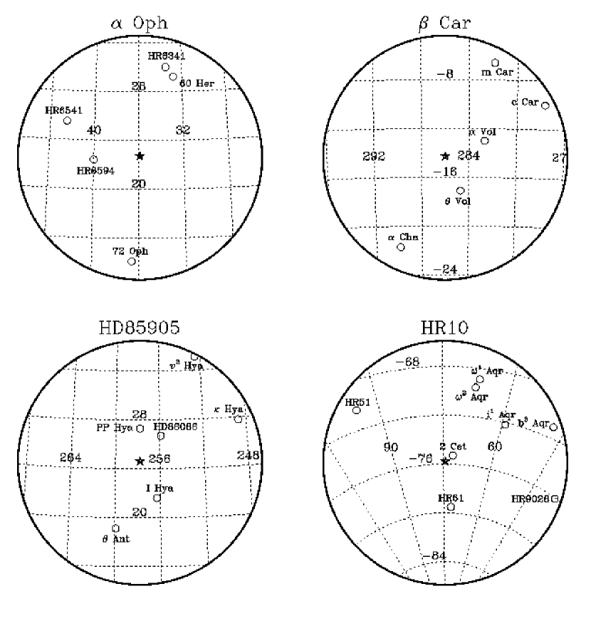
Figure 7: Location of target stars and proximate neighbors in Galactic coordinates. The field of view is 10 degrees radius, centered on the primary target. The distances of the proximate stars bracket the distance of the primary target, but are generally at shorter distances in order to reconstruct the three-dimensional morphology of the LISM in that direction. The stellar properties and coordinates of the proximate stars can be found in Tables 6–9.

Due to the similarity of circumstellar and interstellar absorption signatures, it is important to understand the distribution of interstellar material in the vicinity of our primary targets. For this reason, we observed several stars in close angular proximity and at a range of distances, in order to establish the three-dimensional structure of the ISM in the direction of our primary targets. Tables 6–9 provide the basic stellar parameters of stars proximate to our primary targets, and Figure 7 shows the location of the primary and neighboring stars in Galactic coordinates. If an absorption feature is detected toward both our primary target and a proximate star, it must be located between the Earth and the nearer of the two stars. In particular, the last two columns of Tables 6–9 give the separation of the proximate target from the primary target in angle, $\Delta\theta$, and in distance in the plane of the sky (POS), $\Delta r_{\rm POS}=d_{\rm ISM}\tan(\Delta\theta)$. The distance to the absorbing material, $d_{\rm ISM}$, is rarely known, so the distance to the closer of the two stars is used as an upper limit, $d_{\rm ISM}\leq d_{\star}$. Given the values of $\Delta r_{\rm POS}$ in our proximate star surveys, we may be probing structure on physical scales significantly less than 1 parsec, if the absorbing material is even closer than the nearest of the observed stars. The observational parameters for the proximate stars are given in Table 3.

The LISM is an interstellar environment filled with warm ($T\sim 7000$ K), partially ionized, moderately dense ($n\sim 0.3$ cm^-3) material, surrounded by a volume of hot ($T\sim 10^{6}$ K), rarefied ($n\sim 0.005$ cm^-3) gas known as the Local Bubble. It is relatively common to observe Ca II from the warm partially ionized clouds in the LISM (Redfield & Linsky, 2002), while Na I is rarely detected within the Local Bubble, but is clearly observed in the shell of dense gas that defines its boundary (Lallement et al., 2003). Since the Local Bubble shell is a large scale interstellar structure, it is reasonable to expect that absorption from the Local Bubble will be present in all sightlines that extend beyond its boundary, at $\sim$100 pc. We have used the three-dimensional model of the morphology of the Local Bubble by Lallement et al. (2003), to more carefully estimate the distance to the edge of the Local Bubble in the direction of our 4 primary targets. This is given in 10th column of Table 1. Two of our primary targets, $\alpha$ Oph and $\beta$ Car are well within the Local Bubble and therefore are unlikely to show signatures of absorption from its shell. HD85905 is located just outside the LB shell and therefore, the Na I spectrum is likely to show evidence of ISM absorption due to the LB shell. HR10 is located in the direction of the southern Galactic pole. Due to the lack of dense material in directions perpendicular to the Galactic plane, the Local Bubble is relatively unconfined at its poles (Welsh et al., 1999; Lallement et al., 2003). Therefore, it is unlikely that Local Bubble material will be detected, even in the distant sightlines of HR10 and its proximate stars.

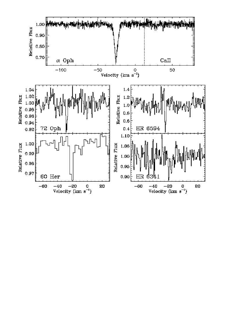
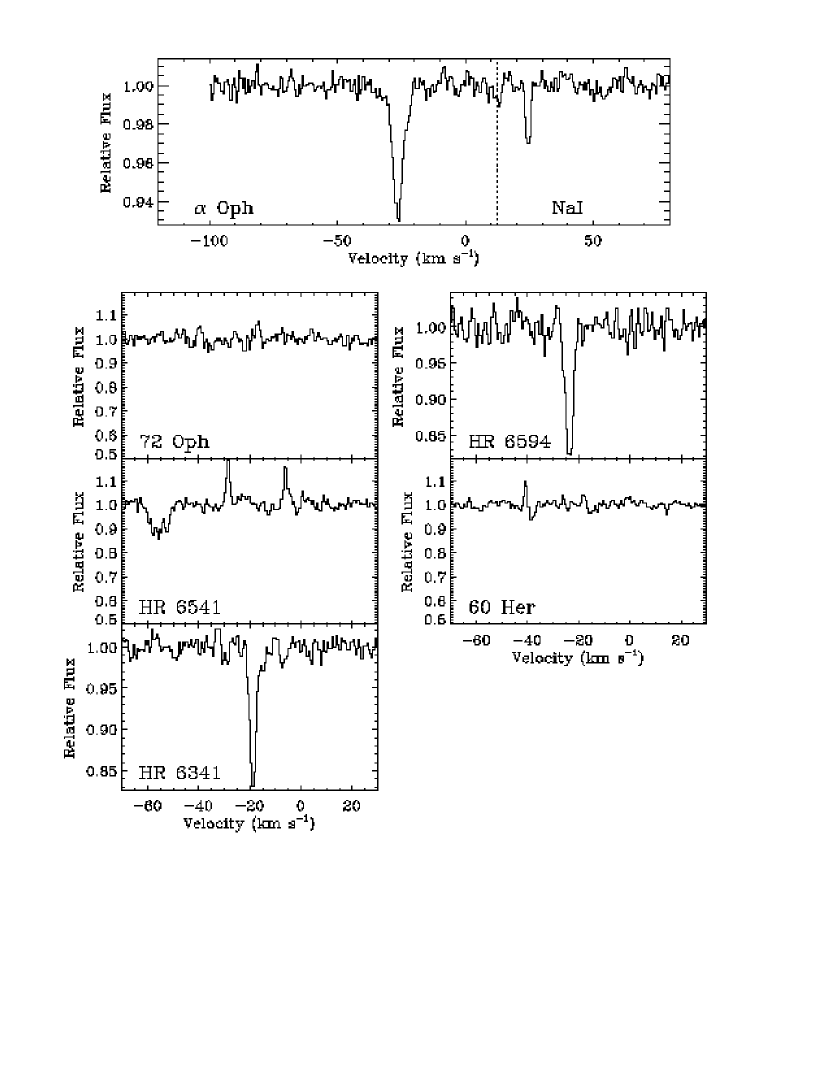
Figure 8: Ca II (left) and Na I (right) absorption lines observed towards stars in close angular proximity to $\alpha$ Oph. Representative spectra of $\alpha$ Oph are provided at the top on the same scale, but with an expanded range. The vertical dotted line indicates the stellar radial velocity. Note the weak atmospheric Na I absorption in the $\alpha$ Oph spectrum near 24.2 km s^-1, well separated from the strong main absorption near –26.6 km s^-1. It is clear that several (4 of 4 in Ca II and 2 of 5 in Na I) proximate targets show absorption at a similar velocity as the main component in $\alpha$ Oph. The Na I spectrum of HR6541 shows signs of the difficulties in measuring weak absorption in this spectral region, including artifacts from the incomplete subtraction of the stellar photospheric Na I line at –55 km s^-1, and overestimated telluric subtraction leading to “emission” spikes at –28 and –6 km s^-1.

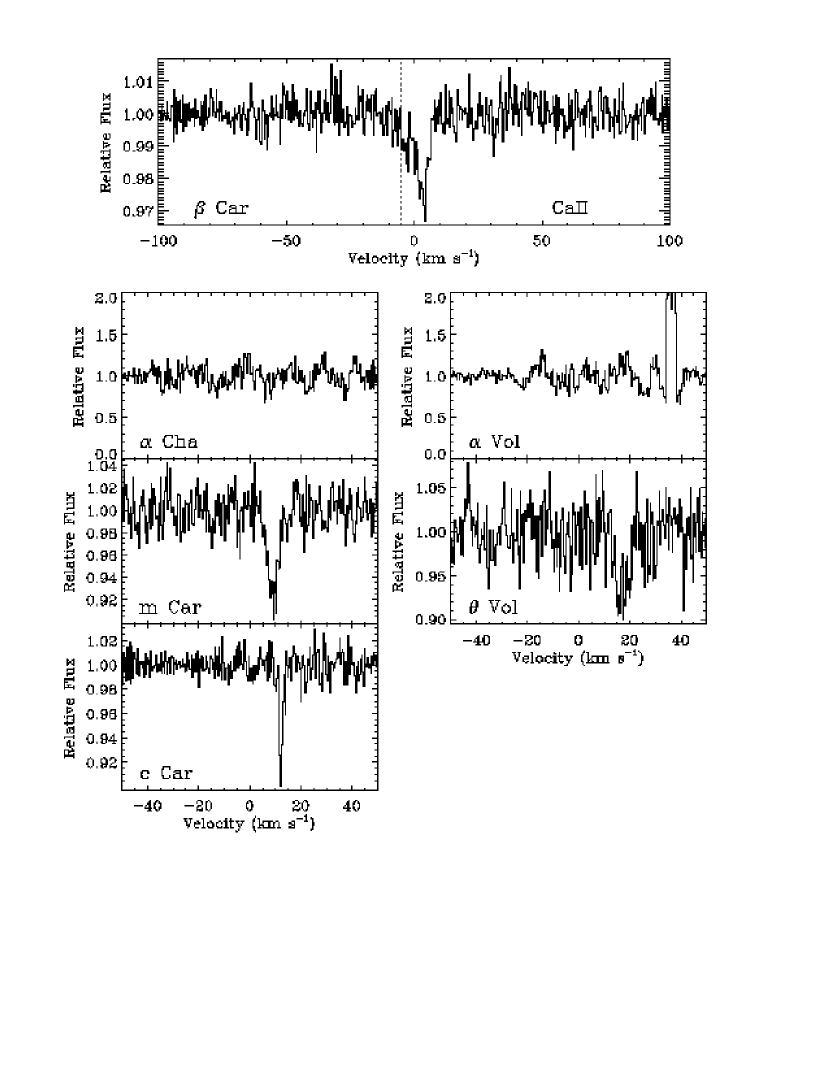
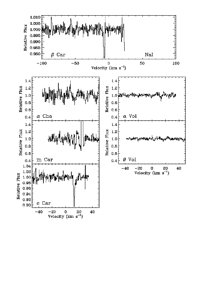
Figure 9: Same as Figure 8 for stars proximate to $\beta$ Car. In this direction, interstellar Ca II is detected in 3 of 5 targets, and Na I detected in only 1 of 5 targets. However the interstellar absorption is consistently redshifted with respect to the absorption detected toward $\beta$ Car. Indeed, the closest star to $\beta$ Car, $\theta$ Vol, shows the largest projected velocity difference in comparison to the absorption toward $\beta$ Car.

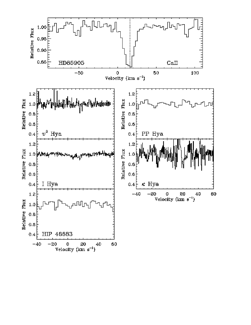
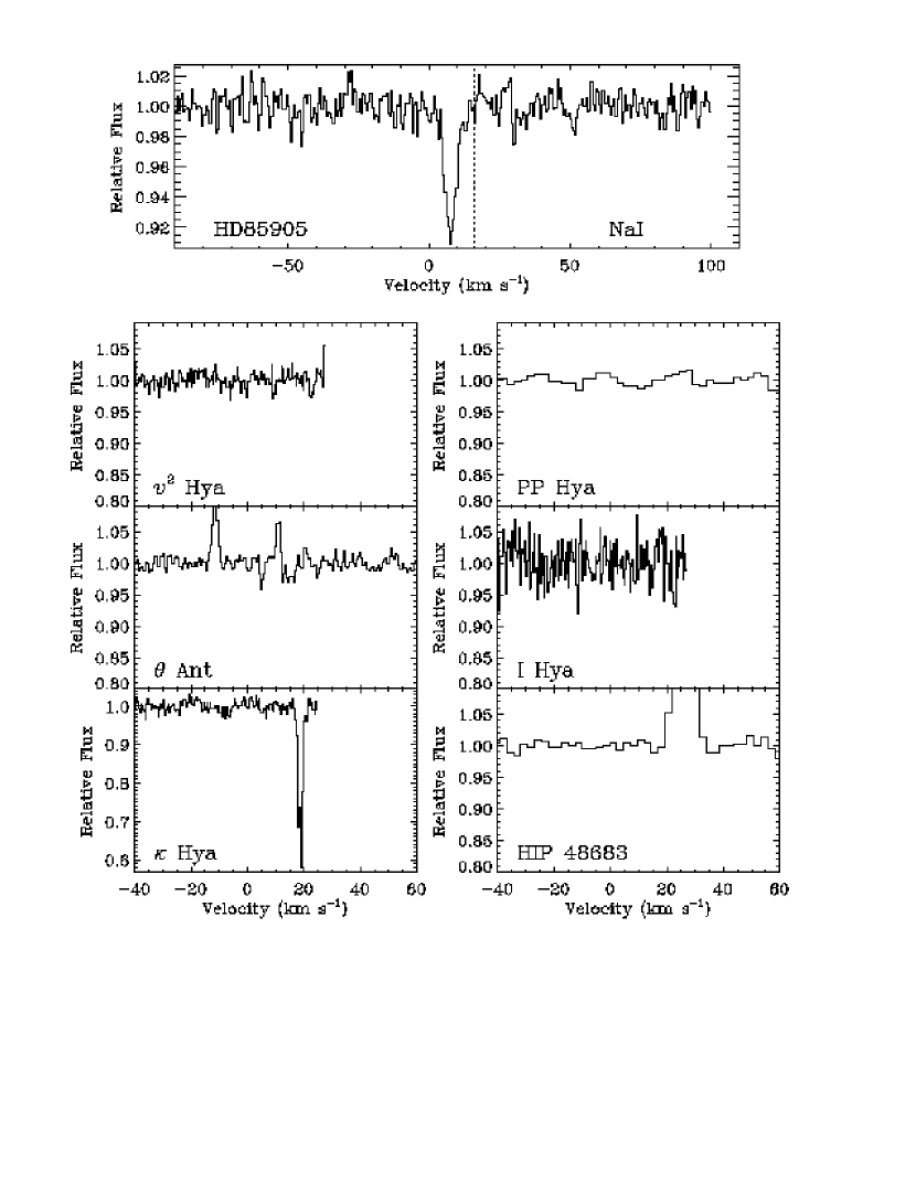
Figure 10: Same as Figure 8 for stars proximate to HD85905. Ca II absorption is not detected toward any of the 5 targets, while Na I is detected in 1 of 6. It is likely that the Na I absorption observed toward HD85905 and $\kappa$ Hya is due to interstellar absorption, even though they show a significant projected velocity difference, due to the large projected separation ($\Delta r_{\rm POS}\leq 22$ pc) between these stars.

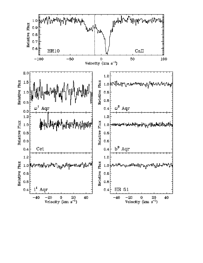
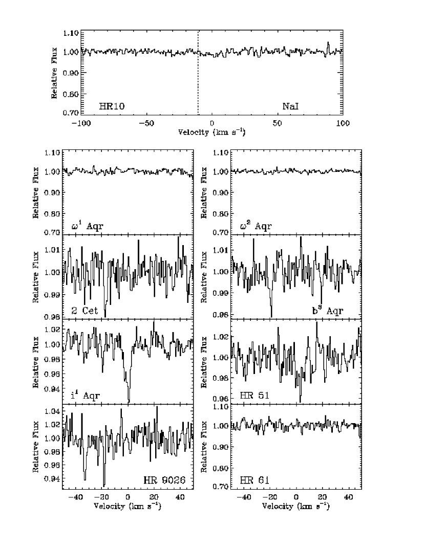
Figure 11: Same as Figure 8 for stars proximate to HR10. No Ca II absorption is detected toward any of 6 targets, while Na I is detected in 5 of 8 targets at two different velocities: near –20 km s^-2 and near 0 km s^-2. Our detection limits in Ca II are significantly lower than the detected absorption in Ca II toward HR10, emphasizing its circumstellar origin.

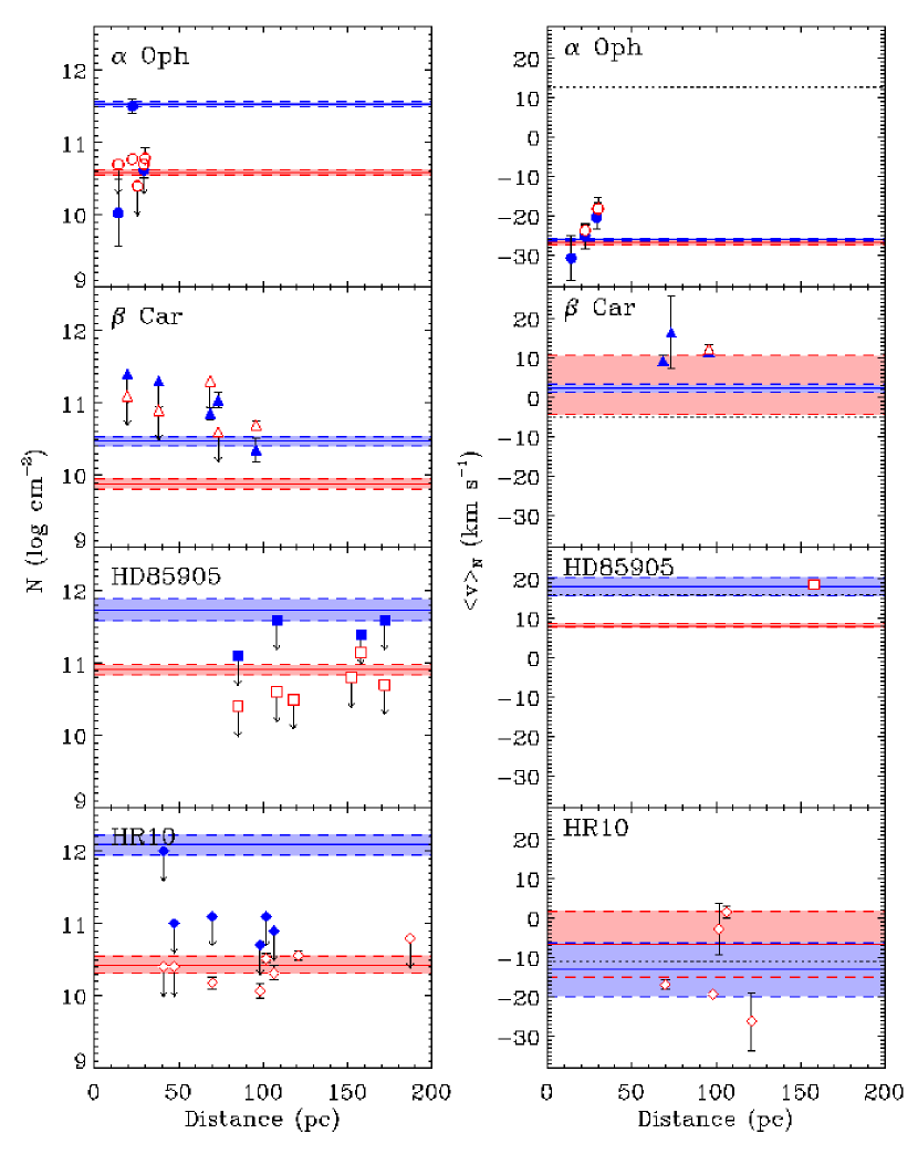
Figure 12: Total column density (left) and column density weighted velocity (right) measurements of absorption toward proximate stars as a function of their distance. The filled symbols indicate Ca II observations, while open symbols indicate Na I. The error bars are the weighted average variance, and in the case of $\langle v\rangle_{N}$ indicate the range of observed velocities rather than the error in measuring the central velocity of absorption. The horizontal dotted line in the right panels indicates the radial velocity of the star. The shaded regions indicate the weighted mean and weighted average variance of the absorption detected in the primary target, as presented in Figure 6 where blue corresponds to Ca II, and red with Na I. The data is also presented in Table 10.

The Ca II and Na I spectral regions for proximate stars are shown in Figures 8–11. In order to maintain small angular distances from our primary targets and to sample a range of pertinent distances, we were severely limited in choice of targets. Often we had to push toward fainter and cooler stars, resulting in lower $S/N$ observations and some contamination by narrow stellar atmospheric lines, respectively. Nonetheless, LISM absorption is clearly detected in several (12/23, 52%) of the targets. The total observed column density and column density weighted velocity for the proximate stars are shown in Figure 12. The weighted average values of our primary stars are plotted as in Figure 6 in order to make a direct comparison.

3.2.1 The LISM Toward $\alpha$ Oph

Inspection of Figures 8 and 12 and Table 10 indicate quite clearly that stars in close proximity to $\alpha$ Oph show absorption in both ions at a similar velocity and strength. Indeed, the nearest star to $\alpha$ Oph, HR6594, only 3.8^∘ away, matches the anomalously high Ca II and Na I column densities seen toward $\alpha$ Oph. The projected distance between $\alpha$ Oph and HR6594 is only 0.9 pc, at the distance of $\alpha$ Oph, which sets the maximum projected distance between the location where these two sightlines probe the absorbing medium. If the absorbing medium is not as distant as $\alpha$ Oph, the projected distance between the sightlines will be even smaller. The other proximate stars that show interstellar absorption, albeit weaker than either $\alpha$ Oph or HR6594, range in projected distance from $\alpha$ Oph from 1.8–2.1 pc in the north-south direction. Because no absorption is detected toward HR6541, 6.7^∘ or 1.7 pc to the northeast, it appears that the morphology of this cloud is quite elongated in the north-south direction, similar to other clouds in the LISM (S. Redfield & J. Linsky 2006, in preparation). A more detailed search would be required to fully delineate the contours of this interesting cloud.

Crawford (2001) presented a similar survey around $\alpha$ Oph, and detected absorption at the same projected velocity as $\alpha$ Oph in 2 of their targets. However, these targets were located at distances of 120-211 pc, a significantly greater distance than $\alpha$ Oph at 14.3 pc. In his ultra high resolution survey, severe restrictions in the brightness of the background star resulted in a survey of targets ranging in distance from 24.1–201 pc, and in angular separation from 0.6–13.2 degrees. Due to the complex morphology of the interstellar medium, particularly at the Local Bubble shell and beyond, which lies only $\sim$55 pc in the direction of $\alpha$ Oph, the observed spectra of distant targets is dominated by distant material, and one becomes in effect “confusion-limited” in terms of identifying weak absorption features, or separating overlapping absorption at coincident projected velocity. We limited the proximate neighbors to distances $<$100 pc, with only one target beyond the Local Bubble, HR6341. Interestingly, only this distant target, and HR6594, the closest star to $\alpha$ Oph, show Na I absorption. Although the absorption toward HR6341 is of comparable strength, it is likely caused by the Local Bubble shell because it is significantly redshifted relative to the strong absorption toward $\alpha$ Oph and HR6594. Our survey, using spectra at lower resolution (but higher $S/N$) than Crawford (2001), was able to retain fainter targets close in both angle and distance to $\alpha$ Oph. Although the LISM absorption toward $\alpha$ Oph remains an outlier in comparison to other nearby stars, our mini-survey of the ISM along its line of sight indicates that the absorption is due to intervening interstellar material $<$14.3 pc from the Sun, rather than circumstellar material surrounding $\alpha$ Oph.

3.2.2 The LISM Toward $\beta$ Car, HD85905, and HR10

The mini-surveys of the LISM near to our remaining 3 targets, $\beta$ Car, HD85905, and HR10, reveal that the majority of absorption observed toward these targets is unlikely to be interstellar.

In the proximity of $\beta$ Car, Na I is detected in only one target, c Car, 95.7 pc, which is also the only target predicted to be beyond the Local Bubble shell located at $\sim$85 pc Lallement et al. (2003). The two shortest sightlines, $\alpha$ Cha and $\alpha$ Vol show no absorption in either ion, but are not sensitive to the low column densities that are detected toward $\beta$ Car. The star nearest in projected distance to $\beta$ Car is $\theta$ Vol. Absorption is detected toward this star, but the central velocity (16.5 km s^-1) is significantly different from that observed toward $\beta$ Car (2.4 km s^-1). Indeed, all absorption detections in proximate neighbors are redshifted by 7–14.1 km s^-1. Figure 7 indicates that since common absorption is detected toward m Car and $\theta$ Vol, which bracket $\beta$ Car and $\alpha$ Vol, it is likely that the interstellar material responsible for the absorption is located 38–69 pc away, between $\alpha$ Vol and m Car. Observations of stars proximate to $\beta$ Car indicate that the absorption observed toward $\beta$ Car is not caused by the LISM.

A significant Ca II column density is detected toward HD85905. None of the observed neighboring stars show any Ca II absorption, despite that the column density upper limits are 1.4–8.7 times lower than the column observed toward HD85905. The same is true for Na I, where the upper limits are 1.3–3.2 times lower. One target, $\kappa$ Hya at a distance of 158 pc, does show Na I absorption. Half of the neighboring stars, and HD85905 itself, are located beyond the predicted Local Bubble shell, which is located at $\sim$120 pc in this direction (Lallement et al., 2003). The two distant neighboring stars that are closest in angular distance from HD85905, I Hya and HIP48683, do not show any indication of Local Bubble shell absorption. However, HD85905 itself, has a constant Na I feature, at a velocity significantly different than the Ca II absorption. It is possible this absorption is due to the Local Bubble shell. However, this requires a patchy morphology of Local Bubble shell material in this direction because HD85905’s nearest neighbors show no Na I absorption and the absorption toward the third distant neighbor is at a different velocity than observed toward HD85905. Regardless of the exact nature of the Na I absorption, it is clear that the Ca II absorption cannot be explained by ISM absorption.

Similar to HD85905, the large Ca II column density observed toward HR10, is not detected in the proximate stars, despite column density upper limits 1.2–25 times lower than observed toward HR10. Very weak Na I absorption is detect both in HR10 and in neighboring stars. Since HR10 is in the direction of the south Galactic pole, and the Local Bubble is relatively unconstrained in this direction (Lallement et al., 2003), no strong Local Bubble absorption is expected. We do start to detect weak absorption at distances $>$70 pc, but the velocity and strength of absorption varies across the 10 degree radius survey area. Three targets show absorption near –20 km s^-1 (2 Cet, b³ Aqr, and HR9026) and two show absorption near 0 km s^-1 (i¹ Aqr and HR51). Some of the Na I detected toward HR10 may be interstellar, but the variability of the Na I absorption toward HR10 indicates much of it is probably circumstellar. Again, it is clear that the Ca II absorption detected toward HR10 is not caused by the ISM along the line of sight.

3.3 Ca II to Na I Ratio

The ratio of Ca II to Na I has been used as a means of discriminating between interstellar and circumstellar material (e.g., Lagrange-Henri et al., 1990b). ISM values are typically low, while those observed toward $\beta$ Pic are much higher, such as $N($Ca II$)/N($Na I$)=38.9\pm 10.9$, as measured by Hobbs et al. (1985), or even $>$100 as seen by Welsh et al. (1997). However, other than for extremely high values (i.e., $>$50), it is difficult to differentiate between circumstellar and interstellar material based on this abundance ratio alone. In the ISM, we see a wide range of Ca II to Na I ratios, some approaching the “high” values seen toward $\beta$ Pic. Welty, Morton, & Hobbs (1996) compile a large sample of ISM measurements, which are dominated by distant sightlines (out to 1 kpc), and find a wide range of Ca II to Na I ratios, from $\sim$0.003 to $\sim$50. Even locally, a wide range of values are measured. For example, Bertin et al. (1993) found 8 stars within 50 pc that showed both Ca II to Na I absorption. Excluding $\alpha$ Oph, the ratio of Ca II to Na I ranges from 2.2–11.9. In general, calcium appears to be more strongly effected by depletion onto dust grains than sodium (Savage & Sembach, 1996). Long sightlines likely sample a wide range of interstellar environments, from cold, dense regions where a significant amount of calcium will be depleted onto dust grains, leading to very low Ca II to Na I ratios, to warm, shocked regions, in which much of the calcium is maintained in the gas phase, and the abundance ratio can be quite high.

Table 10 includes the $N($Ca II$)/N($Na I$)$ ratios for all our circumstellar and interstellar observations. For the three interstellar sightlines that have both Ca II and Na I detections (HR6594, HR6341, and c Car), the ratio ranges from 0.4–5.4. Our circumstellar disk candidates range from 3.9–46. HR10, clearly a variable absorption edge-on disk, has an abundance ratio $N($Ca II$)/N($Na I$)=46^{+23}_{-17}$ at the very high end of the range, comparable with $\beta$ Pic. However, the other three edge-on disk candidates fall well within that found for LISM sightlines (Bertin et al., 1993). $\alpha$ Oph, which we argue is not an edge-on disk, but a particularly small, high column density local cloud, has a moderately high Ca II to Na I ratio, but is consistent with other LISM sightlines. While our other two edge-on disk stars, HD85905 and HR10, which show variability and little indication from neighboring sightlines that they are significantly contaminated by ISM absorption, have relatively high Ca II to Na I ratios, but not extreme enough to clearly differentiate from the general ISM, on the basis of the ratio of Ca II to Na I alone. Note that due to the possibility that some of the constant Na I absorption observed toward HD85905 may be interstellar, the Ca II to Na I ratio given in Table 10 should be considered a lower limit to the circumstellar ratio of these two ions.

3.4 Estimates of Physical Properties of the Variable Circumstellar Gas

The observed temporal variability and lack of comparable absorption in proximate neighbors demonstrates that most of the absorption detected toward our 3 edge-on disk targets ($\beta$ Car, HD85905, and HR10) is due to circumstellar material. These targets have high $v\sin i$ velocities, and are likely viewed edge-on. Since no circumstellar absorption is detected in rapidly rotating intermediate inclination or pole-on debris disks (e.g., Vega and $\alpha$ PsA; Hobbs 1986), it is likely that the circumstellar gas is distributed in an edge-on disk. An edge-on disk morphology is confirmed in infrared and scattered light observations of $\beta$ Pic (Smith & Terrile, 1984; Heap et al., 2000). However, the short and long-term temporal variability in our 3 edge-on disk targets demonstrate that the distribution of material in the gas disk is clumpy.

Our observations are unable to constrain independently the physical size of the absorbing gas structure or its density, other than the absorbing material is presumably very close to the host star in order to cause the observed short term temporal variability. Since we don’t see a particularly stable component centered at the radial velocity of the star, it is unlikely that the gas is smoothly distributed in any extended disk structure, as observed in the stable component of $\beta$ Pic by Brandeker et al. (2004). Instead, it is likely that the absorbing gas is located between approximately 0.3–1.0 AU (Lagrange et al., 2000), and the maximum pathlength is on the order of $\sim$1 AU. If the gas absorption is caused by star-grazing families of evaporating bodies as in the FEB model (Beust, 1994), the pathlength through a gaseous coma-like structure could be significantly less. Although comet comae can reach sizes approaching $\sim$1 AU (Jones et al., 2000), observations of nonblack saturated variable absorption lines toward $\beta$ Pic indicate that the absorbing material does not cover the entire stellar surface and is likely to have a pathlength significantly less than 1 AU (Vidal-Madjar et al., 1994). An upper limit to the amount of variable absorbing gas around $\beta$ Car, HD85905, and HR10 can be estimated if we assume it is distributed in a disk with an inner radius $l_{1}=0.3$ AU and an outer radius of $l_{2}=1.0$ AU. The inner radius ($l_{1}$) is calculated at approximately 0.3 AU, due to the sublimation of most types of grains at distances closer to the host star (Mann et al., 2006; Vidal-Madjar et al., 1986).

In order to convert our observable, $N_{\rm CaII}$, to a hydrogen column density, we use the abundances measured for the stable component of the disk around $\beta$ Pic (Roberge et al., 2006), where the ratio $N($H I$)/N($Ca II$)\lesssim 2.4\times 10^{6}$ is based on $\beta$ Pic Ca II measurements by Crawford et al. (1994) and H I limits by Freudling et al. (1995). The observed Ca II column density is assumed to be caused by circumstellar material only. In this crude upper limit estimate, we assume the largest and simplest configuration of gas closest to the star causing the variable gas absorption. The precise distribution of hydrogen gas in the circumstellar disk is still highly uncertain (Brandeker et al., 2004).

If we assume the morphology of the disk is roughly cylindrical, the total mass in the gas disk can be calculated from,

$$M_{\rm gas}\sim m_{\rm H}\frac{N_{\rm CaII}}{(l_{2}-l_{1})}~{}\frac{N_{\rm HI}}{N_{\rm CaII}}~{}\pi h(l^{2}_{2}-l^{2}_{1})\;\;[{\rm g}]\;,$$ (3)

where $m_{\rm H}$ is the mass of a hydrogen atom, and $h$ is the height of the disk and assumed to be equal to $0.2l_{2}$ (Hobbs et al., 1985). Given the assumptions above, we calculate an upper limit to the total gas mass of the variable component toward $\beta$ Car of $M_{\rm gas}\lesssim 4\times 10^{-9}M_{\oplus}$, HD85905 of $M_{\rm gas}\lesssim 7\times 10^{-8}M_{\oplus}$, and HR10 of $M_{\rm gas}\lesssim 2\times 10^{-7}M_{\oplus}$. In units of $M_{\rm Halley}=10^{17}$ g (Whipple, 1987), the upper limits on the variable gas component mass would be 9000, 4000, 200 $M_{\rm Halley}$, respectively. Note that due to the lack of constraints on the distribution of the absorbing material, these are likely upper limits to the total amount of variable component gas surrounding these stars.

4 Detections and Constraints on Circumstellar Disk Dust

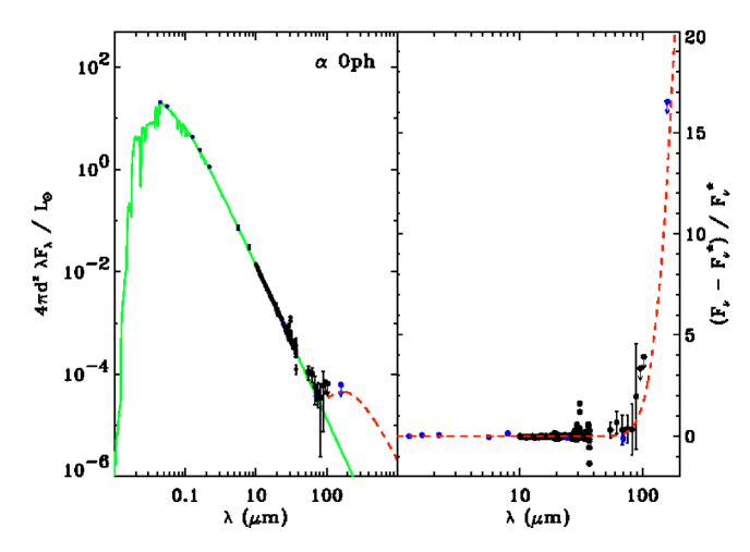
Figure 13: SED (left) and (SED-star)/star (right) for $\alpha$ Oph. Photometry from $B$, $V$, $J$, $H$, and $K$ bands and IRAC and MIPS are shown as blue points, with black error bars overlaid. IRS and MIPSSED spectra are shown in black. NextGen models of stellar photospheres specified by spectral type are overlaid in green. Blackbody fits to the maximum hypothetical excess still allowed by our observations are depicted by red dashed lines.

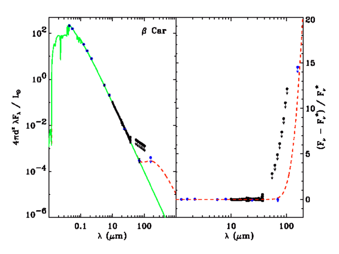
Figure 14: SED (left) and (SED-star)/star (right) for $\beta$ Car. Symbols are the same as in Figure 13.

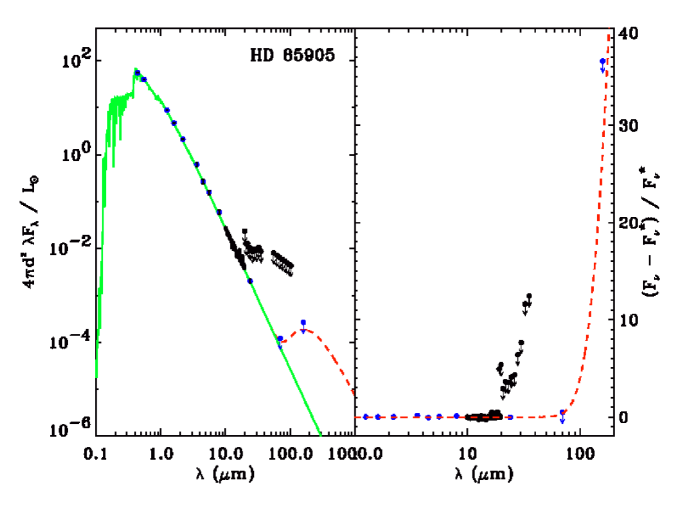
Figure 15: SED (left) and (SED-star)/star (right) for HD85905. Symbols are the same as in Figure 13. IRS LH spectrum was not detected and a single upper limit equal to 3$\times$RMS is plotted for each order. MIPS SED data are outside the plotted region in the right panel.

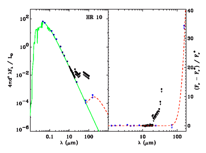
Figure 16: SED (left) and (SED-star)/star (right) for HR10. Symbols are the same as in Figure 13. IRS LH spectrum was not detected and a single upper limit equal to 3$\times$RMS is plotted for each order. MIPS SED data are outside the plotted region in the right panel.

The IR SEDs for all four sources are shown in the left panels of Figures 13–16. These SEDs include $B$, $V$, $J$, $H$, and $K$ bands and IRAC and MIPS photometric data (blue points) as well as IRS and MIPSSED spectra (black lines). $\alpha$ Oph and $\beta$ Car are detected at all bands except 160 $\mu$m, while HR10 and HD85905 are not detected at 70 or 160 $\mu$m. HR10 and HD85905 are also undetected in the IRS LH module, and upper limits, equal to 3$\times$RMS are calculated for each order. The upper limits for MIPS 70 $\mu$m are more constraining than are the upper limits for the LH $\sim 19$–37 $\mu$m data, so the latter are not used for fitting the excess. All 4 sources appear photospheric in all detected bands, so the upper limits for the 70 $\mu$m and/or 160 $\mu$m MIPS bands are used to place upper limits on the temperature and amount of dust that may exist in disks around these stars. All optical and IR photometric measurements used in the SEDs are given in Table Spitzer Limits On Dust Emission and Optical Gas Absorption Variability Around Nearby Stars with Edge-On Circumstellar Disk Signatures.

In order to model a debris disk around our primary targets, we must estimate several stellar parameters, such as effective temperature ($T_{\star}$), luminosity ($L_{\star}$), radius ($R_{\star}$), gravity ($\log g$), mass ($M_{\star}$), and age. The parameters used for our models are listed in Table 12. Two of our primary targets, $\alpha$ Oph and $\beta$ Car, have excellent temperature and radii measurements, and therefore well determined luminosities, since they have been observed from the ultraviolet to the IR, and also have radio angular diameter measurements and accurate distances (Code et al. 1976; Beeckmans 1977; Malagnini et al. 1986; Richichi, Percheron, & Khristoforova 2005). Stellar parameters for our other two primary targets, HD85905 and HR10, are calculated using relations from Napiwotzki, Schoenberner, & Wenske (1993) and Flower (1996). The spectral types were used to estimate the gravity and stellar mass. The age of these systems was estimated using isochrones from Bertelli et al. (1994).

The observed MIPS fluxes (and upper limits) and modeled stellar spectra are used to constrain the amount of excess at dust temperatures comparable to the Asteroid Belt ($T_{dust}=150$–250 K) and Kuiper Belt ($T_{dust}=30$–60 K), using the method described by Bryden et al. (2006). Assuming that the dust in the debris disk is well represented by a single temperature, then the ratio of the observed flux relative to the stellar flux can be used to calculate the ratio of the total dust disk luminosity relative to the stellar luminosity on the Rayleigh-Jeans tail of the stellar blackbody curve,

$$\frac{L_{dust}}{L_{\star}}=\frac{F_{dust}}{F_{\star}}\frac{kT_{dust}^{4}(e^{{h{\nu}/{kT_{dust}}}}-1)}{{h}{\nu}{T_{\star}^{3}}}\;.$$ (4)

Using temperatures of 100, 35, and 15 K, to correspond to blackbody curves peaking at 24, 70 and 160 $\mu$m, we use the following simplified expression to calculate $L_{dust}/L_{\star}$,

$$\frac{L_{dust}}{L_{\star}}=\frac{F_{\lambda,dust}}{F_{\lambda,\star}}\left(\frac{5600K}{T_{\star}}\right)^{3}C_{\lambda}\;,$$ (5)

where $C_{\lambda}$ is a constant that is dependent on the temperature of the dust ($T_{dust}$) and wavelength and equal to $3.7{\times}10^{-4}$, $1.5{\times}10^{-5}$, and $1.3{\times}10^{-6}$ for 24, 70 and 160 $\mu$m, respectively. The flux ratios and resulting $L_{dust}/L_{\star}$ estimates are listed in Table 13. Equation 5 is used to calculate upper limits for $L_{dust}/L_{\star}$ for regions of temperatures corresponding to the 24, 70 and 160 $\mu$m photometry. For the entire sample, we can limit $L_{dust}/L_{\star}$ to less than $\sim$5000 times that of the Asteroid Belt ($L_{dust}/L_{\star}\sim 10^{-8}$ to $10^{-7}$; Dermott et al., 2002), by using the 24 $\mu$m fluxes ($T\approx 100$ K), and we can limit $L_{dust}/L_{\star}$ to less than $\sim$18–30 times that of the Kuiper Belt ($L_{dust}/L_{\star}\sim 10^{-7}$ to $10^{-6}$; Stern, 1996), by using the 70 $\mu$m fluxes ($T\approx 35$ K). For material at lower temperatures than the Kuiper Belt, we can constrain $L_{dust}/L_{\star}$ to less than $\sim$26–66 times that of the Kuiper Belt, using the 160 $\mu$m fluxes ($T\approx 15$ K).

The fractional excess emission ($F_{\nu}^{tot}-F_{\nu}^{star}/F_{\nu}^{star}$) is plotted in the right panels of Figures 13–16. The stellar photospheres are fit using NextGen model atmospheres (Hauschildt, Allard, & Baron, 1999) matching the stellar parameters listed in Table 12 and scaled to match the J-band flux taken from the literature, as the SEDs are clearly photospheric at 1.2 $\mu$m. By making some assumptions about the distribution of the dust contributing to the excess we can also calculate limits on the luminosity of dust in these disks. Once the stellar contribution has been removed, a blackbody function is fit to the excess from $\lambda=1$–160 $\mu$m. As we are interested in calculating the maximum possible excess in these fits, upper limits are ignored if there is a detection or upper limit at longer wavelength with a smaller fractional excess. Fitting the excess with black body function implies that the dust contributing to the excess lies in a ring, of approximately constant temperature ($T_{dust}$), at a corresponding distance, $D=(1/2)(T_{\star}/T_{dust})^{2}R_{\star}$, from the star. The results of the fit, listed in Table 14, are the temperature of the blackbody dust ($T_{dust}$), the solid angle subtended by the dust ($\Omega$) and the reduced $\chi^{2}$ for each source. The excess infrared luminosity is calculated as $L_{IR}=4{\Omega}{\sigma}T_{dust}^{4}d^{2}$, where $d$ is the distance in cm to each source and $\sigma$ is the Stephan-Boltzmann constant. All four sources possess fractional luminosities, listed in Table 14, of $L_{IR}/L_{\star}\leq 5{\times}10^{-6}$, consistent with or less than the fractional luminosities calculated above and similar to the least luminous of known debris disks (Chen et al., 2006).

In order to place limits on the mass of dust surrounding these stars, we need to make some assumptions about the dust properties (see Chen et al., 2006, for a detailed description). First, for simplicity, we assume that the dust is composed primarily of silicates, with a corresponding bulk density (${\rho}_{s}$) of 3.3 g cm^-3. (Note that changing the dust composition to include carbon or silica grains would change the overall bulk density slightly to ${\rho}_{s}=3.5$ g cm^-3 and ${\rho}_{s}=2.3$ g cm^-3 for carbon and silica grains, respectively.) Next we assume that radiation pressure removes grains smaller than $a_{min,0}$, thus setting the minimum grain size. Therefore, we can calculate the mass of small grains with radii equal $a_{min,0}$, using the relation $M_{dust}=(16/3)\pi(L_{IR}/L_{\star})\rho_{s}D^{2}a_{min,0}$ (c.f., Chen et al., 2006, Equation 5). This is a lower limit to the dust surrounding these stars. An upper limit to the mass of dust can be found if we assume that the grain sizes follow the distribution $n_{0}a^{-3.5}$ with a maximum radius of $a_{max}=10$ cm and using the relation $M_{10cm}=(4/3)\rho_{s}\sqrt{a_{min,0}a_{max}}d^{2}\Omega$ (c.f., Chen et al., 2006, Equation 6), where $d$ is the distance in cm to the observed star. As shown in Table 14, the masses of material contributing to the measured excesses from these 4 disks are not particularly small, ranging from $1{\times}10^{-3}$ $M_{\earth}$ to 2 $M_{\earth}$. One must note, however, that this is the mass of dust located at very large radii, $D\sim 1000$-2400 AU from the star. The lack of significant excess at shorter wavelengths, and thus smaller radii, suggests that much of the inner regions of these systems have been effectively cleared, which would increase the difficulty of feeding the variable gas material that is observed around three of these stars, $\beta$ Car, HD85905, and HR10 (see Sec 3.1).

5 Constraints on Circumstellar Bulk Disk Gas

We searched for several IR bulk gas phase atomic lines including Ne II, Ne III, Fe I, Fe II, S I, Si II, as well as 4 ro-vibrational transitions of molecular hydrogen, H₂ S(0)-S(4). Unfortunately, none were detected. Upper limits are presented in Tables 15–16 ($3{\times}RMS{\times}FWHM$, where $FWHM$ is the expected full width at half maximum of an atomic emission line). Upper limits for the masses of gas in these disks are calculated from the H₂ S(0) and H₂ S(1) line upper limits, assuming local thermal equilibrium (LTE) and using excitation temperatures of $T_{ex}=50$ K and 100 K, which are appropriate if the dust and gas are roughly cospatial. The total column density of H₂ gas can be computed as

$$N_{tot}=\frac{F_{ul}\;\lambda_{ul}}{A_{ul}\;h\;c\;{\chi}_{u}}\,\frac{4{\pi}}{\Omega}\;\;[{\rm cm}^{-2}]\;,$$ (6)

where $\lambda_{ul}$, $F_{ul}$, and $A_{ul}$ are the wavelength in cm, observed flux upper limit in erg s^-1 cm^-2, and Einstein A coefficient in s^-1 for the transition, $\Omega$ is the beam solid angle in steradians, and $\chi_{u}$ is the fractional column density of H₂ in the upper level,

$$\chi_{u}=\frac{N_{u}}{N_{tot}}=\frac{(2J+1)\;g{{}_{N}}}{Z(T_{ex})}\,e^{-E_{u}/kT_{ex}}\;.$$ (7)

For H₂ S(0), $A_{ul}=2.94{\times}10^{-11}$ s^-1 and $E_{u}/k=510$ K and for H₂ S(1), $A_{ul}=4.76{\times}10^{-10}$ s^-1 and $E_{u}/k=1015$ K (Wolniewicz, Simbotin, & Dalgarno, 1998). As transitions are restricted to either ortho (parallel nuclear spin) or para (antiparallel nuclear spin) states, if we assume ortho/para ${\approx}$ 3, then $g_{N}=1$ for para transitions, such as H₂ S(0), and $g_{N}=3$ for ortho transitions, such as H₂ S(1). Finally, the total mass of H₂ in the disk can be calculated,

$$M_{tot}=N_{tot}\;m_{H_{2}}\;{\Omega}\;{d^{2}}\;\;[{\rm g}]\;,$$ (8)

where, $m_{H_{2}}$ is the molecular weight of H₂ in grams and $d$ is the distance to the disk in centimeters. The upper limits for the total column densities of H₂ are listed in the last four columns of Table 16. The cold gas mass constraints are $<$2–100 $M_{\oplus}$ for $T=100$ K and $<$200–1$\times$10⁶ $M_{\oplus}$ for $T=50$ K. Note that the H₂ S(1) line is located in a particularly noisy region of the SH spectrum, and thus upper limits are much higher than for H₂ S(0).

The atomic sulfur line (S I) at 25.23 $\mu$m may be a more sensitive tracer of gas mass in low mass disks than H₂. Gorti & Hollenbach (2004) find that for disks around G and K stars, with gas masses of $10^{-3}$–1 $M_{J}$ and dust masses of $10^{-7}$–$10^{-4}$ $M_{J}$, the strength of the S I emission line can be up to 1000 times that of the H₂ S(0) line, if both lines are optically thin. Using a line strength for H₂ S(0) of 1000 times less than the observed S I upper limits, we find that the gas mass could be $\sim$500 times less than the values calculated from H₂ S(0) for $\alpha$ Oph and $\beta$ Car. No estimates can be made for HD85905 and HR10, since these sources were not detected in the LH IRS module, which contains both the S I and H₂ S(0) lines.

6 Discussion

6.1 Circumstellar or Interstellar?

Due to the similarity in spectral profile, a single spectrum is often not sufficient to distinguish whether the absorption is caused by circumstellar or interstellar material, or both. Several techniques have been used to determine the source of absorption. (1) Observations of stars in close angular proximity and similar distance to the primary target can be used to reconstruct the interstellar medium along the line of sight to the primary target (e.g., Crawford, 2001). (2) Repeated observations of the primary target can be used to search for short term absorption variability that is not observed in the large-scale structures of the interstellar medium (e.g, Lagrange-Henri et al., 1990a; Petterson & Tobin, 1999). (3) Observations of transitions, such as metastable lines, that are not observed in the relatively low density interstellar medium can be used to indicate the presence of circumstellar material (e.g., Kondo & Bruhweiler, 1985; Hobbs et al., 1988).

We present results using techniques (1) and (2). The monitoring campaign to search for temporal variability and mini-surveys of stars in close angular proximity to our primary targets, clearly indicate that 3 of our 4 targets are surrounded by circumstellar material. Temporal variability is detected in our observations of $\beta$ Car, HD85905, and HR10, confirming detections of variation in these objects by Lagrange-Henri et al. (1990a), Welsh et al. (1998), and Hempel & Schmitt (2003). In addition, our survey of the ISM in the direction of these targets indicate that little to none of the absorption can be attributed to the interstellar medium. Although it has been speculated that the anomalously high absorption toward $\alpha$ Oph could be caused by circumstellar material, we use nearby stars to firmly identify the interstellar material that is responsible for the absorption toward $\alpha$ Oph, confirming a similar study of more distant stars by Crawford (2001). Future work will entail looking for absorption from metastable lines for our three targets that show evidence for circumstellar gas.

6.2 $\beta$ Pic-like Debris Disk or Be Star-like Stellar Wind Disk?

The origin of the circumstellar gas in edge-on systems that show absorption line variability is a long-standing question. The systems studied in this work may qualify as either weak debris disk systems that currently have variable gas located very close to star but very little dust, or weak winded, rapidly rotating, early type stars that expel gas and form disks similar to classical Be stars.

The objects studied are relatively mature systems, older than $\beta$ Pic (which is $\sim$12 Myr), but roughly contemporaneous with Vega, 0.4 Gyr, and $\epsilon$ Eri, 0.6 Gyr (Zuckerman, 2001). Although most stars at this age have cleared their stellar systems of primordial disk material, several are still in the evolutionary transition period where they have retained a significant amount of secondary dust and gas in their circumstellar surroundings.

The prototypical debris disks mentioned above all have IR excesses, further evidence that the circumstellar material is processed from a protostellar disk. In addition, the one system that is oriented edge-on ($\beta$ Pic) also shows gas absorption. Our targets are all A stars similar to $\beta$ Pic, and 3 of the 4 show gas absorption at levels lower or comparable to $\beta$ Pic (e.g., $N_{\rm CaII}($HR10$)/N_{\rm CaII}(\beta$ Pic$)\sim 0.65$). However, the fractional luminosities caused by an infrared excess consistent with upper limits of the SEDs of our targets are lower than $\beta$ Pic by more than 2 to 3 orders of magnitude (Backman & Paresce, 1993). No stable gas component located at the stellar radial velocity is detected in our targets, which since for $\beta$ Pic, the stable gas appears to be associated with the bulk dust disk (Brandeker et al., 2004), is consistent with our nondetection of any infrared excess. However, there remains the difficulty of feeding a variable gas component, most probably by multitudes of star-grazing planetismal small bodies, without creating an observable secondary dust disk through collisions of the same bodies.

On the other hand, rapidly rotating B stars with strong radiatively driven winds deposit a significant amount of gas into their circumstellar environments. These B stars often have strong emission lines (e.g., hydrogen), and hence are classified as Be stars. The “Be” phenomenon has also been observed in some early A stars and late O stars, but peaks at spectral types B1–B2 (Porter & Rivinius, 2003). A stars can power weak radiatively driven winds, but the mass loss rates are significantly smaller, $\dot{M}<10^{-16}M_{\odot}$ yr^-1, and only metals are expelled (Babel, 1995). Over the ages of the stars studied here, even with such a weak wind, enough mass can be delivered to the circumstellar environment to be consistent with our observations, although it does need to be retained relatively close the star. Our stars do not show any hydrogen emission lines in their optical or infrared spectra, but as rapidly rotating early-type stars, they may be able to produce an irregular circumstellar disk from stellar winds.

Due to the similarity in signatures of gas disks in $\beta$ Pic-like debris disks and Be star-like stellar wind disks, it is important to keep in mind that it is difficult to distinguish the two based on gas absorption lines alone. In a study of rapidly rotating (i.e., edge-on) A stars similar to our sample, Abt et al. (1997) find that $\sim$25% of their stars show Ti II absorption. This is a similar ratio as found for A stars with debris disks at 24 $\mu$m; $\sim$32% (Su et al., 2006). Abt et al. (1997) argue that the observed material cannot be remnants of star formation because they do not observe absorption at all 3 epochs (spanning a total of 22 years) in 3 of their 7 Ti II absorption stars. However, it is plausible that the mechanism causing variability in debris disks, such as $\beta$ Pic, can be dramatic enough to result in nondetections of gas absorption, particularly in weak sources, as 2 of their 3 variable Ti II absorption stars are. Although the similarity of detection fraction in these two studies may be a coincidence, it would be interesting to search for IR excesses around these Ti II absorbers to look for any remnants of protostellar dust.

Detections of dust around our stars that have variable circumstellar gas absorption would have strengthened their identification as debris disk systems rather than stellar outflow disks. However, IR excess nondetections leave the origin of the observed gas disks an open question. The upper limits on the fractional IR luminosity could still be consistent with a debris disk, albeit with much less dust than debris disks like $\beta$ Pic, but still comparable to other Spitzer debris disks (Chen et al., 2006). At the same time, if there is actually little or no dust in these systems, it is quite possible that the origin of the variable circumstellar gas disk is stellar winds. Expanding the sample and further monitoring of the gas content in edge-on systems will help resolve this issue.

7 Conclusions

We present Spitzer infrared photometry and spectroscopy together with high resolution optical spectra of 4 nearby stars that have variable or anomalous optical absorption suspected to be due to circumstellar material. Our findings include:

1. The optical atomic absorption transitions of Ca II and Na I were monitored toward all 4 stars at high spectral resolution. The observational baseline was more than 2.8 years. Absorption line variability was detected in 3 of 4 targets, $\beta$ Car showed variability in Na I while strong Ca II variability was detected toward HD85905 and HR10. Our observations add to previous studies of these same targets by other researchers, which now extends the observed baseline to more than 20 years.

2. Night-to-night variability is detected toward HD85905 and HR10. Although similar to the short term variability detected $\beta$ Pic, the magnitude and frequency of the variations are lower toward HD85905 and HR10.

3. The fraction of the circumstellar absorption that is redshifted relative to the radial velocity of the star ranges from 0–100%. Unlike $\beta$ Pic, the distribution of variable absorption toward our targets is not heavy skewed to the red.

4. Mini-surveys (5–7 stars) of the LISM were conducted within 10^∘ of each primary target. We restricted our sample to stars as close in distance as possible to our primary targets in order to avoid contamination by more distant interstellar material.

5. In the direction of $\alpha$ Oph, we firmly identified the LISM material that causes the anomalously high absorption seen, and thereby show that circumstellar material is not responsible for the observed absorption. In particular, HR6594, the nearest star to $\alpha$ Oph and only 35.5 pc away, shows comparable absorption in Ca II and Na I. Absorption levels drop off rapidly indicating a small and possibly filamentary LISM structure in that direction. The lack of variability and the extremely constraining IR excess measurements support the lack of circumstellar material around $\alpha$ Oph.

6. The LISM in the direction of the other 3 targets, $\beta$ Car, HD85905, and HR10, is responsible for little to none of the observed absorption. Only the constant Na I feature see toward HD85905, may be caused by material in the Local Bubble shell, and unrelated to the circumstellar material around HD85905.

7. The Ca II to Na I ratio is measured for all stars. Only HR10 shows an extremely high ratio, consistent with some of the high values seen toward $\beta$ Pic. The other targets show levels that are high, but not inconsistent with LISM and circumstellar measurements. Unless $N($Ca II$)/N($Na I$)\gg 10$, the variation in the interstellar ratio make it difficult to use this ratio alone to determine if the absorbing material is circumstellar or interstellar. In this respect, the observed targets differ significantly from $\beta$ Pic, which shows a strong IR excess and stable gas absorption component.

8. We search for IR excesses with Spitzer in all 4 stars that have shown variable or anomalous optical absorption. We do not detect any significant IR excesses in IRAC or MIPS photometry or IRS spectroscopy, in any of the targets. This is consistent with no detection of a stable gas component at rest in the stellar reference frame.

9. Sensitive measurements of the IR SEDs provide strong constraints on the maximum possible dust luminosities (i.e., consistent with the Spitzer upper limits at the longest IR wavelengths) of these systems. Fractional luminosity upper limits range from 1.8 to $5.4\times 10^{-6}$, and are several orders of magnitude lower than measured for $\beta$ Pic, despite that the gas absorption line column densities are only slightly lower than those observed toward $\beta$ Pic.

10. No molecular hydrogen lines are detected in the IRS spectra, nor are any atomic transitions detected. Limits on the integrated line fluxes for important transitions are provided.

11. We estimate upper limits to the mass of the variable gas component causing the optical atomic absorption, that range from 0.4 to 20 $\times 10^{-8}M_{\oplus}$. Combined with the nondetection and tight constraints on any dust in these systems, the source of the variable gas component remains an open question. If evaporation of small star-grazing objects are responsible for the variable gas absorption, they are not contributing significantly to any dusty debris disk.

Table 1: Stellar Properties of Primary Targets

HD	Other	Spectral	$m_{\rm V}$	$v_{\rm R}$	$v\sin i$	$l$	$b$	Distance	Dist. to LB Boundary
#	Name	Type	(mag)	(km s-1)	(km s-1)	(deg)	(deg)	(pc)	(pc)
159561	$\alpha$ Oph	A5III	2.10	12.6	228	35.9	22.6	14.32${}^{+0.18}_{-0.18}$	$\sim$55
80007	$\beta$ Car	A2IV	1.70	–5	145	286.0	–14.4	34.08${}^{+0.55}_{-0.54}$	$\sim$85
85905	HR3921	A2/A3III	6.23	16	264	257.8	24.5	140${}^{+15}_{-13}$	$\sim$120
256	HR10	A2IV/V	6.23	–10.8	241	74.36	–75.9	160${}^{+25}_{-19}$	$>$250

Table 2: Observational Parameters for Primary Stars

HD	Other	Date	Telescope	Instrument	Ion	$v_{\rm atm}$	Exposure	$S/N$
#	Name					(km s-1)	(s)
159561	$\alpha$ Oph	2003 Oct 6	McD2.7	CS12	CaII	$\cdots$	3600	42
159561	$\alpha$ Oph	2004 Apr 7	McD2.7	CS12	CaII	$\cdots$	2400	36
159561	$\alpha$ Oph	2004 Aug 27	McD2.7	CS21	CaII	$\cdots$	1800	227
159561	$\alpha$ Oph	2004 Aug 27	McD2.7	CS21	CaII	$\cdots$	1800	112
159561	$\alpha$ Oph	2004 Aug 28	McD2.7	CS21	CaII	$\cdots$	1800	263
159561	$\alpha$ Oph	2004 Aug 28	McD2.7	CS21	CaII	$\cdots$	1800	136
159561	$\alpha$ Oph	2004 Aug 29	McD2.7	CS21	CaII	$\cdots$	1800	115
159561	$\alpha$ Oph	2004 Aug 30	McD2.7	CS21	CaII	$\cdots$	1800	156
159561	$\alpha$ Oph	2004 Oct 18	McD2.7	CS21	CaII	$\cdots$	1200	245
159561	$\alpha$ Oph	2005 Feb 14	McD2.7	CS21	CaII	$\cdots$	900	118
159561	$\alpha$ Oph	2005 Feb 15	McD2.7	CS21	CaII	$\cdots$	1800	126
159561	$\alpha$ Oph	2005 Feb 15	McD2.7	CS21	NaI	+22.1	2400	160
159561	$\alpha$ Oph	2005 Feb 28	AAT3.9	UHRF	NaI	+23.7	2400	123
159561	$\alpha$ Oph	2005 Mar 14	McD2.7	CS21	CaII	$\cdots$	600	76
159561	$\alpha$ Oph	2005 Mar 16	McD2.7	CS21	CaII	$\cdots$	1200	181
159561	$\alpha$ Oph	2005 Mar 16	McD2.7	CS21	NaI	+24.2	1200	336
159561	$\alpha$ Oph	2005 Mar 17	McD2.7	CS21	CaII	$\cdots$	1200	201
159561	$\alpha$ Oph	2005 Mar 17	McD2.7	CS21	NaI	+24.2	600	230
159561	$\alpha$ Oph	2005 Mar 21	McD2.7	CS12	CaII	$\cdots$	2400	27
159561	$\alpha$ Oph	2005 Mar 22	McD2.7	CS12	CaII	$\cdots$	1200	27
159561	$\alpha$ Oph	2005 Mar 23	McD2.7	CS12	CaII	$\cdots$	1800	19
159561	$\alpha$ Oph	2005 Jun 12	AAT3.9	UHRF	CaII	$\cdots$	3600	52
159561	$\alpha$ Oph	2005 Jun 14	AAT3.9	UHRF	NaI	–0.4	2700	57
159561	$\alpha$ Oph	2005 Jun 15	AAT3.9	UHRF	CaII	$\cdots$	6000	58
159561	$\alpha$ Oph	2005 Jul 15	McD2.7	CS21	CaII	$\cdots$	600	143
159561	$\alpha$ Oph	2005 Jul 18	McD2.7	CS12	CaII	$\cdots$	2700	31
159561	$\alpha$ Oph	2005 Jul 19	McD2.7	CS12	NaI	–13.7	2700	66
159561	$\alpha$ Oph	2005 Aug 18	AAT3.9	UHRF	CaII	$\cdots$	2400	60
159561	$\alpha$ Oph	2005 Sep 11	McD2.7	CS12	CaII	$\cdots$	1200	33
159561	$\alpha$ Oph	2005 Sep 14	McD2.7	CS21	CaII	$\cdots$	600	167
159561	$\alpha$ Oph	2006 Feb 13	McD2.7	CS12	CaII	$\cdots$	3600	19
159561	$\alpha$ Oph	2006 Feb 14	McD2.7	CS21	CaII	$\cdots$	1200	138
159561	$\alpha$ Oph	2006 Feb 14	McD2.7	CS21	NaI	+21.9	900	359
159561	$\alpha$ Oph	2006 Jul 6	AAT3.9	UHRF	CaII	$\cdots$	2400	33
80007	$\beta$ Car	2005 Feb 25	AAT3.9	UHRF	CaII	$\cdots$	2400	144
80007	$\beta$ Car	2005 Feb 26	AAT3.9	UHRF	CaII	$\cdots$	2400	152
80007	$\beta$ Car	2005 Feb 26	AAT3.9	UHRF	NaI	+23.5	1200	111
80007	$\beta$ Car	2005 Feb 28	AAT3.9	UHRF	CaII	$\cdots$	1200	105
80007	$\beta$ Car	2005 Feb 28	AAT3.9	UHRF	NaI	+23.7	1800	103
80007	$\beta$ Car	2005 Mar 1	AAT3.9	UHRF	NaI	+23.8	1200	124
80007	$\beta$ Car	2005 Jun 12	AAT3.9	UHRF	CaII	$\cdots$	2400	103
80007	$\beta$ Car	2005 Jun 15	AAT3.9	UHRF	CaII	$\cdots$	2700	112
80007	$\beta$ Car	2005 Jun 15	AAT3.9	UHRF	NaI	–0.6	2700	214
80007	$\beta$ Car	2005 Aug 16	AAT3.9	UHRF	CaII	$\cdots$	1500	65
80007	$\beta$ Car	2006 Jul 5	AAT3.9	UHRF	CaII	$\cdots$	1200	102
85905	HR3921	2004 Dec 2	McD2.7	CS23	CaII, NaI	+28.2	1800	41, 224
85905	HR3921	2004 Dec 6	McD2.7	CS23	CaII, NaI	+27.5	1800	46, 237
85905	HR3921	2005 Feb 14	McD2.7	CS21	CaII	$\cdots$	2700	30
85905	HR3921	2005 Feb 14	McD2.7	CS21	NaI	–1.5	1800	55
85905	HR3921	2005 Feb 26	AAT3.9	UHRF	CaII	$\cdots$	3600	17
85905	HR3921	2005 Mar 1	AAT3.9	UHRF	CaII	$\cdots$	3600	17
85905	HR3921	2005 Mar 1	AAT3.9	UHRF	NaI	–8.7	3600	37
85905	HR3921	2005 Mar 14	McD2.7	CS21	CaII	$\cdots$	2700	28
85905	HR3921	2005 Mar 14	McD2.7	CS21	NaI	–15.1	2700	44
85905	HR3921	2005 Mar 16	McD2.7	CS21	NaI	–16.0	2400	51
85905	HR3921	2005 Mar 17	McD2.7	CS21	CaII	$\cdots$	4500	44
85905	HR3921	2005 Mar 17	McD2.7	CS21	NaI	–16.4	2700	60
85905	HR3921	2005 Jun 15	AAT3.9	UHRF	NaI	–24.8	4800	27
85905	HR3921	2006 Feb 14	McD2.7	CS21	CaII	$\cdots$	3600	17
85905	HR3921	2006 Feb 14	McD2.7	CS21	NaI	–1.4	2400	97
256	HR10	2004 Aug 27	McD2.7	CS21	CaII	$\cdots$	2700	30
256	HR10	2004 Aug 27	McD2.7	CS21	NaI	+15.4	2700	103
256	HR10	2004 Aug 28	McD2.7	CS21	CaII	$\cdots$	900	13
256	HR10	2004 Aug 28	McD2.7	CS21	NaI	+15.0	2700	97
256	HR10	2004 Oct 18	McD2.7	CS21	CaII	$\cdots$	5400	31
256	HR10	2004 Oct 18	McD2.7	CS21	NaI	–9.1	2700	94
256	HR10	2004 Oct 19	McD2.7	CS21	NaI	–9.6	2700	131
256	HR10	2004 Oct 20	McD2.7	CS21	NaI	–10.0	2700	102
256	HR10	2005 Jun 15	AAT3.9	UHRF	CaII	$\cdots$	5400	10
256	HR10	2005 Jul 15	McD2.7	CS21	NaI	+27.3	1200	56
256	HR10	2005 Sep 14	McD2.7	CS21	CaII	$\cdots$	3600	54
256	HR10	2005 Sep 14	McD2.7	CS21	NaI	+7.5	2400	90

Table 3: Observational Parameters for Stars in Close Proximity to Primary Targets

HD	Other	Date	Telescope	Instrument	Ion	$v_{\rm atm}$	Exposure	$S/N$
#	Name					(km s-1)	(s)
165777	72 Oph	2004 Aug 27	McD2.7	CS21	CaII	$\cdots$	2700	147
165777	72 Oph	2004 Oct 20	McD2.7	CS21	NaI	–22.4	1200	59
165777	72 Oph	2005 Jun 15	AAT3.9	UHRF	CaII	$\cdots$	3300	23
165777	72 Oph	2005 Sep 9	McD2.7	CS12	CaII	$\cdots$	7200	19
160910	HR6594	2004 Aug 28	McD2.7	CS21	CaII	$\cdots$	1800	28
160910	HR6594	2005 Jul 16	McD2.7	CS21	NaI	–11.5	1200	54
159332	HR6541	2005 Jul 17	McD2.7	CS21	NaI	–12.3	1200	50
154494	60 Her	2004 Oct 20	McD2.7	CS21	CaII	$\cdots$	1200	16
154494	60 Her	2004 Oct 20	McD2.7	CS21	NaI	–17.2	1200	41
154494	60 Her	2005 Jun 30	McD2.7	CS23	CaII, NaI	–10.3	1800	172, 826
154494	60 Her	2005 Jul 19	McD2.7	CS12	NaI	–16.7	3600	10
154494	60 Her	2005 Sep 14	McD2.7	CS21	NaI	–23.8	600	76
154494	60 Her	2005 Sep 14	McD2.7	CS21	CaII	$\cdots$	1800	55
154494	60 Her	2006 Jul 3	AAT3.9	UHRF	CaII	$\cdots$	7200	27
154228	HR6341	2005 Jun 12	AAT3.9	UHRF	CaII	$\cdots$	4800	10
154228	HR6341	2005 Jul 16	McD2.7	CS21	CaII	$\cdots$	1800	46
154228	HR6341	2005 Jul 16	McD2.7	CS21	NaI	–15.8	1800	99
71243	$\alpha$ Cha	2005 Jun 14	AAT3.9	UHRF	NaI	+28.2	3600	12
71243	$\alpha$ Cha	2006 Jul 5	AAT3.9	UHRF	CaII	$\cdots$	3300	13
78045	$\alpha$ Vol	2005 Feb 26	AAT3.9	UHRF	CaII	$\cdots$	2700	32
78045	$\alpha$ Vol	2005 Feb 26	AAT3.9	UHRF	NaI	–14.9	2700	27
83944	m Car	2005 Feb 26	AAT3.9	UHRF	CaII	$\cdots$	2700	47
83944	m Car	2005 Feb 26	AAT3.9	UHRF	NaI	–14.8	2400	17
74405	$\theta$ Vol	2005 Jun 15	AAT3.9	UHRF	NaI	+28.3	3600	34
74405	$\theta$ Vol	2006 Mar 19	AAT3.9	UHRF	CaII	$\cdots$	2400	32
76728	c Car	2005 Feb 25	AAT3.9	UHRF	NaI	–15.3	2700	70
76728	c Car	2005 Feb 26	AAT3.9	UHRF	CaII	$\cdots$	1800	71
76728	c Car	2005 Feb 28	AAT3.9	UHRF	CaII	$\cdots$	1800	71
87504	$\upsilon^{2}$ Hya	2005 Jan 28	McD2.7	CS12	CaII	$\cdots$	6000	13
87504	$\upsilon^{2}$ Hya	2005 Mar 1	AAT3.9	UHRF	NaI	–13.6	2700	61
87504	$\upsilon^{2}$ Hya	2005 Mar 1	AAT3.9	UHRF	CaII	$\cdots$	3600	19
87130	PP Hya	2004 Dec 6	McD2.7	CS23	CaII, NaI	+28.1	1200	24, 163
84367	$\theta$ Ant	2006 Feb 15	McD2.7	CS21	NaI	–4.0	2400	111
83953	I Hya	2005 Mar 1	AAT3.9	UHRF	NaI	–13.6	1200	22
83953	I Hya	2005 Mar 1	AAT3.9	UHRF	CaII	$\cdots$	2700	33
83754	$\kappa$ Hya	2005 Mar 1	AAT3.9	UHRF	NaI	–13.6	1800	50
83754	$\kappa$ Hya	2005 Jun 12	AAT3.9	UHRF	CaII	$\cdots$	3600	10
86066	HIP48683	2004 Dec 6	McD2.7	CS23	CaII, NaI	+27.9	600	17, 95
222345	$\omega^{1}$ Aqr	2005 Jul 17	McD2.7	CS21	CaII	$\cdots$	600	13
222345	$\omega^{1}$ Aqr	2005 Jul 17	McD2.7	CS21	NaI	+25.7	1200	84
222661	$\omega^{2}$ Aqr	2005 Jul 15	McD2.7	CS21	CaII	$\cdots$	1800	47
222661	$\omega^{2}$ Aqr	2005 Jul 15	McD2.7	CS21	NaI	+26.2	1200	125
222661	$\omega^{2}$ Aqr	2005 Jul 18	McD2.7	CS12	CaII	$\cdots$	4800	14
222661	$\omega^{2}$ Aqr	2005 Jul 19	McD2.7	CS12	NaI	+25.4	2700	17
225132	2 Cet	2004 Oct 20	McD2.7	CS21	NaI	–10.4	1200	150
225132	2 Cet	2005 Jul 18	McD2.7	CS12	CaII	$\cdots$	3600	12
225132	2 Cet	2005 Jul 19	McD2.7	CS12	NaI	+26.5	3600	18
221565	b3 Aqr	2004 Oct 19	McD2.7	CS21	NaI	–11.9	1200	149
221565	b3 Aqr	2004 Oct 19	McD2.7	CS21	CaII	$\cdots$	1200	21
221565	b3 Aqr	2005 Aug 14	AAT3.9	UHRF	CaII	$\cdots$	2400	32
222847	i1 Aqr	2004 Oct 20	McD2.7	CS21	NaI	–12.1	1200	84
222847	i1 Aqr	2004 Oct 20	McD2.7	CS21	CaII	$\cdots$	1200	26
1064	HR51	2005 Sep 15	McD2.7	CS21	CaII	$\cdots$	1200	49
1064	HR51	2005 Sep 15	McD2.7	CS21	NaI	+6.6	1200	82
223466	HR9026	2004 Oct 19	McD2.7	CS21	NaI	–9.2	1200	63
1256	HR61	2004 Oct 20	McD2.7	CS21	NaI	–8.4	1200	53

Table 4: Spitzer Observations

	IRAC		MIPS		IRS		MIPSSED
Source	AOR Key	Date	AOR Key	Date	AOR Key	Date	AOR Key	Date
$\alpha$ Oph	11026688	2004 Sep 03	11026176	2005 Apr 09	11026944	2004 Sep 28	11026432	2005 Sep 26
$\beta$ Car	11027712	2005 Jan 20	11027200, 13658624	2005 Jan 28, 2005 May 20	11027968	2005 Jan 13	11027456	2005 Sep 26
HD85905	11029760	2004 Dec 17	11029248, 13658880	2004 Dec 04, 2005 May 20	11030016	2004 Dec 09	11029504	2005 Sep 26
HR10	11028736	2004 Nov 25	11028224, 13658368	2004 Dec 05, 2005 Jun 23	11028992	2005 Jun 30	11028480	2005 Sep 26

Table 5: High Resolution Absorption Line Measurement History

HD	Other	Ion	Date	$\langle v\rangle_{N}$	$\log N$	Reference
#	Name			(km s-1)	(cm-2)
159561	$\alpha$ Oph	CaII	2006 Jul 06	$-25.7\pm 2.3$	$11.49\pm 0.04$	this work
159561	$\alpha$ Oph	CaII	2006 Feb 14	$-26.1\pm 2.7$	$11.55\pm 0.01$	this work
159561	$\alpha$ Oph	CaII	2006 Feb 13	$-25.7\pm 2.1$	$11.44\pm 0.02$	this work
159561	$\alpha$ Oph	CaII	2005 Sep 14	$-26.1\pm 2.7$	$11.57\pm 0.01$	this work
159561	$\alpha$ Oph	CaII	2005 Sep 11	$-25.8\pm 2.6$	$11.51\pm 0.01$	this work
159561	$\alpha$ Oph	CaII	2005 Aug 18	$-25.9\pm 2.5$	$11.50\pm 0.02$	this work
159561	$\alpha$ Oph	CaII	2005 Jul 18	$-25.5\pm 2.1$	$11.52\pm 0.01$	this work
159561	$\alpha$ Oph	CaII	2005 Jul 15	$-26.0\pm 2.4$	$11.53\pm 0.01$	this work
159561	$\alpha$ Oph	CaII	2005 Jun 15	$-26.0\pm 2.5$	$11.49\pm 0.02$	this work
159561	$\alpha$ Oph	CaII	2005 Jun 12	$-25.7\pm 2.9$	$11.46\pm 0.03$	this work
159561	$\alpha$ Oph	CaII	2005 Mar 23	$-25.2\pm 3.1$	$11.47\pm 0.01$	this work
159561	$\alpha$ Oph	CaII	2005 Mar 22	$-25.1\pm 3.9$	$11.47\pm 0.01$	this work
159561	$\alpha$ Oph	CaII	2005 Mar 21	$-25.7\pm 2.1$	$11.48\pm 0.01$	this work
159561	$\alpha$ Oph	CaII	2005 Mar 17	$-26.3\pm 2.6$	$11.55\pm 0.01$	this work
159561	$\alpha$ Oph	CaII	2005 Mar 16	$-26.0\pm 2.5$	$11.53\pm 0.01$	this work
159561	$\alpha$ Oph	CaII	2005 Mar 14	$-25.7\pm 3.1$	$11.51\pm 0.02$	this work
159561	$\alpha$ Oph	CaII	2005 Feb 15	$-25.8\pm 2.2$	$11.52\pm 0.01$	this work
159561	$\alpha$ Oph	CaII	2005 Feb 14	$-25.6\pm 3.0$	$11.53\pm 0.01$	this work
159561	$\alpha$ Oph	CaII	2004 Oct 18	$-26.2\pm 2.5$	$11.52\pm 0.01$	this work
159561	$\alpha$ Oph	CaII	2004 Aug 30	$-26.1\pm 2.3$	$11.53\pm 0.01$	this work
159561	$\alpha$ Oph	CaII	2004 Aug 29	$-25.9\pm 2.1$	$11.52\pm 0.01$	this work
159561	$\alpha$ Oph	CaII	2004 Aug 28	$-26.1\pm 2.6$	$11.55\pm 0.01$	this work
159561	$\alpha$ Oph	CaII	2004 Aug 27	$-26.0\pm 2.7$	$11.56\pm 0.01$	this work
159561	$\alpha$ Oph	CaII	2004 Apr 07	$-25.6\pm 2.5$	$11.46\pm 0.01$	this work
159561	$\alpha$ Oph	CaII	2003 Oct 06	$-25.3\pm 2.1$	$11.50\pm 0.01$	this work
159561	$\alpha$ Oph	CaII	2002 Mar 26	$-25$	$11.30$	Hempel & Schmitt (2003)
159561	$\alpha$ Oph	CaII	1996 Feb 29	$\cdots$	$11.37$	Hempel & Schmitt (2003)
159561	$\alpha$ Oph	CaII	1994 Apr 24	$-26.3\pm 2.4$	$11.54\pm 0.07$	Crawford (2001)
159561	$\alpha$ Oph	CaII	1994 Apr 24	$-26.1\pm 2.1$	$11.38^{+0.12}_{-0.18}$	Crawford & Dunkin (1995)
159561	$\alpha$ Oph	CaII	1993 Sep 28 – 1993 Oct 01	$-26.5$	11.53	Welty et al. (1996)
159561	$\alpha$ Oph	CaII	1984–1986	$-25.3\pm 1.0$	$11.40\pm 0.02$	Lallement, Vidal-Madjar, & Ferlet (1986)
159561	$\alpha$ Oph	NaI	2006 Feb 14	$-26.3\pm 2.5$	$10.58\pm 0.01$	this work
159561	$\alpha$ Oph	NaI	2005 Jul 19	$-27.1\pm 0.8$	$10.46\pm 0.05$	this work
159561	$\alpha$ Oph	NaI	2005 Jun 14	$-26.0\pm 1.3$	$10.48\pm 0.08$	this work
159561	$\alpha$ Oph	NaI	2005 Mar 17	$-26.2\pm 2.1$	$10.58\pm 0.02$	this work
159561	$\alpha$ Oph	NaI	2005 Mar 16	$-26.3\pm 2.4$	$10.62\pm 0.01$	this work
159561	$\alpha$ Oph	NaI	2005 Feb 28	$-25.6\pm 3.0$	$10.63\pm 0.05$	this work
159561	$\alpha$ Oph	NaI	2005 Feb 15	$-25.6\pm 2.3$	$10.57\pm 0.04$	this work
159561	$\alpha$ Oph	NaI	1991–1992	$-26.4\pm 1.0$	$10.48\pm 0.03$	Bertin et al. (1993)
159561	$\alpha$ Oph	NaI	1987–1989	$-25.8$	$10.45$	Welty et al. (1994)
80007	$\beta$ Car	CaII	2006 Jul 05	$2.8\pm 2.3$	$10.46\pm 0.10$	this work
80007	$\beta$ Car	CaII	2005 Aug 16	$3.1\pm 1.5$	$10.18\pm 0.32$	this work
80007	$\beta$ Car	CaII	2005 Jun 15	$0.5\pm 4.3$	$10.38\pm 0.12$	this work
80007	$\beta$ Car	CaII	2005 Jun 12	$1.2\pm 3.2$	$10.51\pm 0.10$	this work
80007	$\beta$ Car	CaII	2005 Feb 28	$1.5\pm 3.3$	$10.56\pm 0.08$	this work
80007	$\beta$ Car	CaII	2005 Feb 26	$1.8\pm 2.9$	$10.49\pm 0.06$	this work
80007	$\beta$ Car	CaII	2005 Feb 25	$1.3\pm 5.0$	$10.47\pm 0.07$	this work
80007	$\beta$ Car	CaII	2002 Mar 27	$4.0$	$10.14$	Hempel & Schmitt (2003)
80007	$\beta$ Car	CaII	2002 Mar 26	$4.0$	$10.14$	Hempel & Schmitt (2003)
80007	$\beta$ Car	CaII	1996 Feb 29	$\cdots$	$10.50$	Hempel & Schmitt (2003)
80007	$\beta$ Car	NaI	2005 Jun 15	$-7.1\pm 0.6$	$9.87\pm 0.13$	this work
80007	$\beta$ Car	NaI	2005 Mar 01	$7.3\pm 0.6$	$10.14\pm 0.12$	this work
80007	$\beta$ Car	NaI	2005 Feb 28	$7.0\pm 0.6$	$10.15\pm 0.14$	this work
80007	$\beta$ Car	NaI	2005 Feb 26	$7.2\pm 0.6$	$9.96\pm 0.21$	this work
80007	$\beta$ Car	NaI	1989–1991	$\cdots$	$<$10.23	Welsh et al. (1994)
85905	HR3921	CaII	2006 Feb 14	$19.2\pm 7.2$	$11.39\pm 0.06$	this work
85905	HR3921	CaII	2005 Mar 17	$15.9\pm 11.0$	$11.62\pm 0.05$	this work
85905	HR3921	CaII	2005 Mar 14	$19.3\pm 3.8$	$11.86\pm 0.01$	this work
85905	HR3921	CaII	2005 Mar 01	$20.2\pm 4.2$	$11.46\pm 0.08$	this work
85905	HR3921	CaII	2005 Feb 26	$12.4\pm 12.2$	$11.77\pm 0.04$	this work
85905	HR3921	CaII	2005 Feb 14	$16.1\pm 7.3$	$11.78\pm 0.03$	this work
85905	HR3921	CaII	2004 Dec 06	$15.7\pm 5.0$	$11.65\pm 0.02$	this work
85905	HR3921	CaII	2004 Dec 02	$13.7\pm 8.5$	$11.91\pm 0.01$	this work
85905	HR3921	CaII	1997 Nov 17	$7.0$	$11.97$	Welsh et al. (1998)
85905	HR3921	CaII	1997 Jan 25	$-11.5$	$12.24$	Welsh et al. (1998)
85905	HR3921	CaII	1997 Jan 24	$-5.9$	$11.99$	Welsh et al. (1998)
85905	HR3921	CaII	1987 May	$\cdots$	$11.97^{+0.05}_{-0.06}$	Lagrange-Henri et al. (1990b)
85905	HR3921	NaI	2006 Feb 14	$7.8\pm 3.2$	$11.02\pm 0.01$	this work
85905	HR3921	NaI	2005 Jun 15	$5.7\pm 7.3$	$10.90\pm 0.09$	this work
85905	HR3921	NaI	2005 Mar 17	$7.7\pm 1.2$	$10.92\pm 0.03$	this work
85905	HR3921	NaI	2005 Mar 16	$8.4\pm 1.6$	$10.99\pm 0.03$	this work
85905	HR3921	NaI	2005 Mar 14	$8.4\pm 1.8$	$10.86\pm 0.04$	this work
85905	HR3921	NaI	2005 Mar 01	$9.3\pm 1.6$	$10.97\pm 0.05$	this work
85905	HR3921	NaI	2005 Feb 14	$7.9\pm 1.4$	$10.91\pm 0.02$	this work
85905	HR3921	NaI	2004 Dec 06	$7.6\pm 2.6$	$10.93\pm 0.01$	this work
85905	HR3921	NaI	2004 Dec 02	$8.0\pm 3.2$	$10.82\pm 0.01$	this work
85905	HR3921	NaI	1997 Nov 19	$9.2$	$11.22$	Welsh et al. (1998)
85905	HR3921	NaI	1997 Jan 26	$-10.8$	$11.06$	Welsh et al. (1998)
256	HR10	CaII	2005 Sep 14	$1.8\pm 12.1$	$12.19\pm 0.01$	this work
256	HR10	CaII	2005 Jun 15	$1.6\pm 6.9$	$12.44\pm 0.02$	this work
256	HR10	CaII	2004 Oct 18	$-11.4\pm 10.4$	$12.04\pm 0.01$	this work
256	HR10	CaII	2004 Aug 28	$-10.1\pm 10.7$	$11.87\pm 0.06$	this work
256	HR10	CaII	2004 Aug 27	$-15.9\pm 2.6$	$11.95\pm 0.03$	this work
256	HR10	CaII	1997 Nov 18	$6.1$	$12.23$	Welsh et al. (1998)
256	HR10	CaII	1997 Nov 17	$2.7$	$12.14$	Welsh et al. (1998)
256	HR10	CaII	1997 Jun 20	$4.4$	$11.92$	Welsh et al. (1998)
256	HR10	CaII	1997 Jan 25	$-5.1$	$12.55$	Welsh et al. (1998)
256	HR10	CaII	1997 Jan 24	$-6.8$	$12.62$	Welsh et al. (1998)
256	HR10	CaII	1996 Nov 30	$-6.5$	$11.87$	Welsh et al. (1998)
256	HR10	CaII	1986 Aug – 1988 Dec	$\cdots$	$12.09^{+0.04}_{-0.05}$	Lagrange-Henri et al. (1990b)
256	HR10	CaII	1985 Jun – 1985 Oct	$\cdots$	$12.28$	Hobbs (1986)
256	HR10	NaI	2005 Sep 14	$1.4\pm 9.4$	$10.13\pm 0.16$	this work
256	HR10	NaI	2005 Jul 15	$\cdots$	$<$10.5	this work
256	HR10	NaI	2004 Oct 20	$-15.2\pm 10.4$	$10.41\pm 0.05$	this work
256	HR10	NaI	2004 Oct 19	$-7.5\pm 8.0$	$10.44\pm 0.04$	this work
256	HR10	NaI	2004 Oct 18	$-20.5\pm 9.5$	$10.46\pm 0.05$	this work
256	HR10	NaI	2004 Aug 28	$-2.4\pm 7.4$	$10.31\pm 0.09$	this work
256	HR10	NaI	2004 Aug 27	$0.1\pm 8.8$	$10.59\pm 0.05$	this work
256	HR10	NaI	1997 Nov 20	$12.5$	$11.09$	Welsh et al. (1998)
256	HR10	NaI	1997 Nov 19	$-6.9$	$11.49$	Welsh et al. (1998)
256	HR10	NaI	1986 Aug – 1988 Dec	$\cdots$	$<$10.5	Lagrange-Henri et al. (1990b)
256	HR10	NaI	1985 Jun – 1985 Oct	$\cdots$	$<$11.0	Hobbs (1986)

Table 6: Stellar Parameters for Targets Near $\alpha$ Oph

HD	Other	Spectral	$m_{\rm V}$	$v_{\rm R}$	$v\sin i$	$l$	$b$	Distance	$\Delta\theta$	$\Delta r_{\rm POS}$
#	Name	Type	(mag)	(km s-1)	(km s-1)	(deg)	(deg)	(pc)	(deg)	(pc)
165777	72 Oph	A4IVs	3.72	–23.9	65	36.6	14.1	25.38${}^{+0.55}_{-0.52}$	8.53	2.1
160910	HR6594	F4Vw	5.55	–43.7	30	40.0	22.4	35.5${}^{+1.1}_{-1.0}$	3.79	0.9
159332	HR6541	F6V	5.66	–58.8	5	42.5	25.5	36.7${}^{+1.0}_{-1.0}$	6.69	1.7
154494	60 Her	A4IV	4.88	–4.2	117	32.8	29.2	44.1${}^{+1.4}_{-1.4}$	7.16	1.8
154228	HR6341	A1V	5.92	–31.7	43	33.5	30.0	80.8${}^{+4.8}_{-4.3}$	7.71	1.9

Table 7: Stellar Parameters for Targets Near $\beta$ Car

HD	Other	Spectral	$m_{\rm V}$	$v_{\rm R}$	$v\sin i$	$l$	$b$	Distance	$\Delta\theta$	$\Delta r_{\rm POS}$
#	Name	Type	(mag)	(km s-1)	(km s-1)	(deg)	(deg)	(pc)	(deg)	(pc)
71243	$\alpha$ Cha	F5III	4.07	–13.7	0	289.9	–21.7	19.46${}^{+0.19}_{-0.18}$	8.19	2.8
78045	$\alpha$ Vol	A2.5IVm	4.00	4.9	34	282.7	–13.0	38.11${}^{+0.76}_{-0.73}$	3.50	2.1
83944	m Car	B9IV-V	4.51	20	68	281.9	–6.6	68.6${}^{+2.3}_{-2.1}$	8.78	5.3
74405	$\theta$ Vol	A0V	5.19	13	$\cdots$	284.7	–17.1	73.3${}^{+2.8}_{-2.6}$	2.98	1.8
76728	c Car	B8.5II	3.80	25	0	277.7	–10.0	95.7${}^{+4.5}_{-4.1}$	9.23	5.5

Table 8: Stellar Parameters for Targets Near HD85905

HD	Other	Spectral	$m_{\rm V}$	$v_{\rm R}$	$v\sin i$	$l$	$b$	Distance	$\Delta\theta$	$\Delta r_{\rm POS}$
#	Name	Type	(mag)	(km s-1)	(km s-1)	(deg)	(deg)	(pc)	(deg)	(pc)
87504	$\upsilon^{2}$ Hya	B8V	4.59	28	50	252.5	33.1	85.0${}^{+6.1}_{-5.3}$	9.77	14.6
87130	PP Hya	A3III	6.83	$\cdots$	$\cdots$	257.8	27.3	108.1${}^{+12.1}_{-9.9}$	2.80	5.3
84367	$\theta$ Ant	A8V+…	4.79	24.0	$\cdots$	259.9	19.1	117.8${}^{+11.1}_{-9.3}$	5.77	11.9
83953	I Hya	B5V	4.75	25.9	240	256.3	21.6	152${}^{+17}_{-14}$	3.21	8
83754	$\kappa$ Hya	B4IV/V	5.05	18	150	248.7	27.8	158${}^{+27}_{-20}$	8.81	22
86066	HIP48683	A2V	7.43	$\cdots$	$\cdots$	255.9	26.7	172${}^{+26}_{-20}$	2.79	7

Table 9: Stellar Parameters for Targets Near HR10

HD	Other	Spectral	$m_{\rm V}$	$v_{\rm R}$	$v\sin i$	$l$	$b$	Distance	$\Delta\theta$	$\Delta r_{\rm POS}$
#	Name	Type	(mag)	(km s-1)	(km s-1)	(deg)	(deg)	(pc)	(deg)	(pc)
222345	$\omega^{1}$ Aqr	A7IV	4.99	–2	105	67.0	–68.9	41.0${}^{+1.5}_{-1.4}$	7.34	5.3
222661	$\omega^{2}$ Aqr	B9V	4.48	3	142	67.7	–69.6	47.3${}^{+2.0}_{-1.9}$	6.60	5.5
225132	2 Cet	B9IVn	4.54	–5	200	72.1	–75.3	69.9${}^{+4.8}_{-4.2}$	0.83	1.0
221565	b3 Aqr	A0V	4.71	15	180	47.9	–71.1	98.2${}^{+7.8}_{-6.7}$	8.81	15.2
222847	i1 Aqr	B9V	5.24	14	310	59.2	–72.2	101.7${}^{+9.9}_{-8.3}$	5.55	9.9
1064	HR51	B9V	5.76	16.9	124	95.1	–70.4	106.4${}^{+9.6}_{-8.2}$	8.06	15.1
223466	HR9026	A3V	6.42	16.5	70	36.9	–76.1	121${}^{+15}_{-12}$	8.92	19
1256	HR61	B6III/IV	6.49	19	150	72.1	–79.5	187${}^{+36}_{-26}$	3.63	10

Table 10: Absorption Line Properties

HD	Other	$\langle v\rangle_{\rm CaII}$	$\log N_{\rm CaII}$	$\langle v\rangle_{\rm NaI}$	$\log N_{\rm NaI}$	CaII/NaI
#	Name	(km s-1)	(cm-2)	(km s-1)	(cm-2)
159561	$\alpha$ Oph	$-25.8\pm 0.3$	$11.53\pm 0.03$	$-26.6\pm 0.6$	$10.59\pm 0.04$	$8.7\pm 1.0$
165777	72 Oph	$-30.6\pm 5.7$	$10.03\pm 0.47$	$\cdots$	$<$10.7	$>$0.2
160910	HR6594	$-25.0\pm 3.2$	$11.50\pm 0.10$	$-23.6\pm 1.2$	$10.77\pm 0.06$	$5.4^{+1.6}_{-1.3}$
159332	HR6541	$\cdots$	$\cdots$	$\cdots$	$<$10.4	$\cdots$
154494	60 Her	$-20.3\pm 2.8$	$10.62\pm 0.11$	$\cdots$	$<$10.7	$>$0.8
154228	HR6341	$-18.2\pm 1.5$	$10.78\pm 0.16$	$-18.1\pm 2.7$	$10.78\pm 0.02$	$1.0^{+0.4}_{-0.3}$
80007	$\beta$ Car	$2.4\pm 0.9$	$10.47\pm 0.07$	$3.1\pm 7.5$	$9.88\pm 0.07$	$3.9^{+1.0}_{-0.8}$
71243	$\alpha$ Cha	$\cdots$	$<$11.4	$\cdots$	$<$11.1	$\cdots$
78045	$\alpha$ Vol	$\cdots$	$<$11.3	$\cdots$	$<$10.9	$\cdots$
83944	m Car	$9.4\pm 1.2$	$10.85\pm 0.09$	$\cdots$	$<$11.3	$>$0.4
74405	$\theta$ Vol	$16.5\pm 9.1$	$11.04\pm 0.11$	$\cdots$	$<$10.6	$>$2.8
76728	c Car	$11.6\pm 0.5$	$10.35\pm 0.16$	$12.3\pm 1.1$	$10.70\pm 0.05$	$0.4^{+0.2}_{-0.1}$
85905	HR3921	$18.0\pm 2.4$	$11.74\pm 0.15$	$8.2\pm 0.6$	$10.91\pm 0.07$	$6.8^{+3.0}_{-2.2}$
87504	$\upsilon^{2}$ Hya	$\cdots$	$<$11.1	$\cdots$	$<$10.4	$\cdots$
87130	PP Hya	$\cdots$	$<$11.6	$\cdots$	$<$10.6	$\cdots$
84367	$\theta$ Ant	$\cdots$	$\cdots$	$\cdots$	$<$10.5	$\cdots$
83953	I Hya	$\cdots$	$<$10.8	$\cdots$	$<$10.8	$\cdots$
83754	$\kappa$ Hya	$\cdots$	$<$11.4	$18.6\pm 0.7$	$11.15\pm 0.03$	$<$1.8
86066	HIP48683	$\cdots$	$<$11.6	$\cdots$	$<$10.7	$\cdots$
256	HR10	$-13.0\pm 6.8$	$12.09\pm 0.14$	$-6.5\pm 8.3$	$10.43\pm 0.12$	$46^{+23}_{-17}$
222345	$\omega^{1}$ Aqr	$\cdots$	$<$12.0	$\cdots$	$<$10.4	$\cdots$
222661	$\omega^{2}$ Aqr	$\cdots$	$<$11.0	$\cdots$	$<$10.4	$\cdots$
225132	2 Cet	$\cdots$	$<$11.1	$-16.8\pm 1.1$	$10.18\pm 0.08$	$<$8.3
221565	b3 Aqr	$\cdots$	$<$10.7	$-19.2\pm 0.3$	$10.07\pm 0.10$	$<$4.3
222847	i1 Aqr	$\cdots$	$<$11.1	$-2.8\pm 6.6$	$10.52\pm 0.06$	$<$3.8
1064	HR51	$\cdots$	$<$10.9	$1.64\pm 1.5$	$10.32\pm 0.10$	$<$3.8
223466	HR9026	$\cdots$	$\cdots$	$-26.2\pm 7.4$	$10.56\pm 0.06$	$\cdots$
1256	HR61	$\cdots$	$\cdots$	$\cdots$	$<$10.8	$\cdots$

Table 11: IR Flux Measurements

	$B$	$V$	$J$	$H$	$K$	$F_{3.6}$	$F_{4.5}$	$F_{5.8}$	$F_{8.0}$	$F_{24}$	$F_{70}$	$F_{160}$
Source	(mag)	(mag)	(mag)	(mag)	(mag)	(mJy)	(mJy)	(mJy)	(mJy)	(mJy)	(mJy)	(mJy)
$\alpha$ Oph	2.22(3)	2.07(3)	1.75(4)	1.67(3)	1.64(3)	sat.	sat.	2.5E+4(2)	1.5E+4(1)	1.4E+3(1)	1.5E+2(3)	$<$5.9E+2
$\beta$ Car	1.68(1)	1.68(2)	1.55(2)	1.55(1)	1.53(1)	sat.	sat.	2.9E+4(3)	1.5E+4(2)	1.6E+3(2)	1.9E+2(4)	$<$6.0E+2
HD85905	6.27(1)	6.23(1)	6.05(2)	6.04(3)	6.04(2)	1.2E+03(1)	6.6E+02(7)	4.9E+2(5)	2.6E+2(3)	2.7E+1(3)	$<$4.7E+0	$<$2.3E+1
HR10	6.33(1)	6.23(1)	5.86(2)	5.83(3)	5.75(3)	1.6E+03(2)	8.0E+02(8)	5.7E+2(6)	3.2E+2(3)	3.3E+1(3)	$<$4.7E+0	$<$2.6E+1

Note. — The numbers in parentheses note the error in the last significant digit.

References. — $B$ and $V$ photometric data are from SIMBAD. Near-IR $J$, $H$, $K$ fluxes are from the 2 Micron All Sky Survey (2MASS) for HD85905 and HR10, from Alonso, Arribas, & Martinez-Roger (1994) for $\alpha$ Oph, and Bouchet, Schmider, & Manfroid (1991) for $\beta$ Car.

Table 12: Estimated Stellar Parameters

	$T_{\star}$	$L_{\star}$	$R_{\star}$		$M_{\star}$	$\log$ Age
Source	(K)	($L_{\sun}$)	($R_{\sun}$)	$\log{g}$	($M_{\sun}$)	(yr)
$\alpha$ Oph	7980	22.6	2.5	3.8	2.7	9.0
$\beta$ Car	9280	220.5	5.8	3.6	3.6	8.6
HD85905	8840	51.8	3.1	3.3	3.6	8.8
HR10	8370	63.8	3.8	4.1	2.5	8.9

Table 13: Constraints on Excess Luminosity from Photometry

	24$\mu$m			70$\mu$m			160$\mu$m
Source	$F_{\star}$	$F_{MIPS}$/$F_{\star}$	$L_{dust}$/$L_{\star}$	$F_{\star}$	$F_{MIPS}$/$F_{\star}$	$L_{dust}$/$L_{\star}$	$F_{\star}$	$F_{MIPS}$/$F_{\star}$	$L_{dust}$/$L_{\star}$
$\alpha$ Oph	1.5	0.95	2.5E-4	0.17	0.89	9.4E-06	3.4E-2	$<$18	$<$1.6E-05
$\beta$ Car	1.7	0.92	2.1E-4	0.20	0.97	8.8E-06	3.9E-2	$<$16	$<$1.2E-05
HD85905	2.8E-2	0.97	2.3E-4	3.2E-3	$<$1.5	$<$1.4E-05	6.3E-4	$<$38	$<$3.1E-05
HR10	3.3E-2	1.01	2.5E-4	3.8E-3	$<$1.2	$<$1.2E-05	7.4E-4	$<$35	$<$3.1E-05

Table 14: Constraints on Excess Luminosity from Complete SED

	$T_{dust}$	$\Omega$	BB Min.		$D$	$<{a}>$	$M_{dust}$	$M_{10cm}$
Source	(K)	($10^{-14}$ sr${}^{-1})$	$\chi^{2}$	$L_{IR}/L_{\star}$	(AU)	($\mu$m)	($M_{\earth}$)	($M_{\earth}$)
$\alpha$ Oph	21$\pm$2	300$\pm$200	8.8	2.9E-06	900	3.2	6.7E-4	0.15
$\beta$ Car	22$\pm$2	200$\pm$200	5.3	1.7E-06	2400	24	2.0E-2	1.7
HD85905	22$\pm$5	9$\pm$7	23	4.8E-06	1100	5.5	3.2E-3	0.55
HR10	20$\pm$4	17$\pm$6	18	6.1E-06	1600	9.8	1.4E-2	1.8

Table 15: Constraints on Atomic Line Fluxes from IRS

	Ne II	Ne III	Fe I	Fe II	Fe II	S I	Si II
Source	12.814 $\mu$m	15.56 $\mu$m	24.042 $\mu$m	17.936 $\mu$m	25.988 $\mu$m	25.249 $\mu$m	34.820 $\mu$m
	(erg s-1cm-2)	(erg s-1cm-2)	(erg s-1cm-2)	(erg s-1cm-2)	(erg s-1cm-2)	(erg s-1cm-2)	(erg s-1cm-2)
$\alpha$ Oph	$<$2.24E-13	$<$8.62E-14	$<$1.61E-14	$<$4.69E-14	$<$1.08E-14	$<$1.12E-14	$<$4.73E-15
$\beta$ Car	$<$2.49E-13	$<$9.54E-14	$<$1.67E-14	$<$5.19E-14	$<$1.16E-14	$<$1.18E-14	$<$5.12E-15
HD85905	$<$4.38E-15	$<$1.77E-15	…	$<$1.11E-15	…	…	…
HR10	$<$5.67E-15	$<$2.34E-15	…	$<$1.53E-15	…	…	…

Table 16: Constraints on Molecular Hydrogen Line Fluxes from IRS

	H2 S(0)	H2 S(1)	H2 S(2)	H2 S(3)	50 K	100 K	50 K	100 K
Source	28.221 $\mu$m	17.035 $\mu$m	12.279 $\mu$m	9.665 $\mu$m	$M_{H_{2}}$ S(0)	$M_{H_{2}}$ S(0)	$M_{H_{2}}$ S(1)	$M_{H_{2}}$ S(1)
	(erg s-1cm-2)	(erg s-1cm-2)	(erg s-1cm-2)	(erg s-1cm-2)	(M⊕)	(M⊕)	(M⊕)	(M⊕)
$\alpha$ Oph	$<$8.76E-15	$<$5.86E-14	$<$2.60E-13	$<$3.91E-13	$<$200	$<$2	$<$3E+05	$<$20
$\beta$ Car	$<$8.57E-15	$<$6.51E-14	$<$2.90E-13	$<$4.36E-13	$<$1000	$<$10	$<$2E+06	$<$100
HD85905	$<$1.45E-15	$<$1.26E-15	$<$5.08E-15	$<$7.22E-15	…	…	$<$5E+05	$<$40
HR10	$<$1.07E-15	$<$1.75E-15	$<$6.54E-15	$<$8.89E-15	…	…	$<$1E+06	$<$80

References

- Abt & Morrell (1995) Abt, H. A., & Morrell, N. I. 1995, ApJS, 99, 135
- Abt et al. (1997) Abt, H. A., Tan, H., & Zhou, H. 1997, ApJ, 487, 365
- Alonso et al. (1994) Alonso, A., Arribas, S., & Martinez-Roger, C. 1994, A&AS, 107, 365
- Aumann (1985) Aumann, H. H. 1985, PASP, 97, 885
- Babel (1995) Babel, J. 1995, A&A, 301, 823
- Backman & Paresce (1993) Backman, D. E., & Paresce, F. 1993, in Protostars and Planets III, ed. E. H. Levy & J. I. Lunine, 1253–1304
- Barrado y Navascues (1998) Barrado y Navascues, D. 1998, A&A, 339, 831
- Beeckmans (1977) Beeckmans, F. 1977, A&A, 60, 1
- Beichman et al. (2006) Beichman, C. A., et al. 2006, ApJ, 639, 1166
- Bertelli et al. (1994) Bertelli, G., Bressan, A., Chiosi, C., Fagotto, F., & Nasi, E. 1994, A&AS, 106, 275
- Bertin et al. (1993) Bertin, P., Lallement, R., Ferlet, R., & Vidal-Madjar, A. 1993, A&A, 278, 549
- Beust (1994) Beust, H. 1994, in Circumstellar Dust Disks and Planet Formation, ed. R. Ferlet & A. Vidal-Madjar (Gif sur Yvette Cedex: Editions Frontières), 35
- Beust & Morbidelli (2000) Beust, H., & Morbidelli, A. 2000, Icarus, 143, 170
- Bevington & Robinson (1992) Bevington, P. R., & Robinson, D. K. 1992, Data Reduction and Error Analysis for the Physical Sciences, 2nd edn. (New York: McGraw-Hill)
- Bouchet et al. (1991) Bouchet, P., Schmider, F. X., & Manfroid, J. 1991, A&AS, 91, 409
- Brandeker et al. (2004) Brandeker, A., Liseau, R., Olofsson, G., & Fridlund, M. 2004, A&A, 413, 681
- Bryden et al. (2006) Bryden, G., et al. 2006, ApJ, 636, 1098
- Chen et al. (2005) Chen, C. H., et al. 2005, ApJ, 634, 1372
- Chen et al. (2006) —. 2006, ApJS, 166, 351
- Cheng et al. (1992) Cheng, K.-P., Bruhweiler, F. C., Kondo, Y., & Grady, C. A. 1992, ApJ, 396, L83
- Code et al. (1976) Code, A. D., Bless, R. C., Davis, J., & Brown, R. H. 1976, ApJ, 203, 417
- Crawford (2001) Crawford, I. A. 2001, MNRAS, 327, 841
- Crawford et al. (1998) Crawford, I. A., Beust, H., & Lagrange, A.-M. 1998, MNRAS, 294, L31
- Crawford & Dunkin (1995) Crawford, I. A., & Dunkin, S. K. 1995, MNRAS, 273, 219
- Crawford et al. (1994) Crawford, I. A., Spyromilio, J., Barlow, M. J., Diego, F., & Lagrange, A. M. 1994, MNRAS, 266, L65
- Dermott et al. (2002) Dermott, S. F., Durda, D. D., Grogan, K., & Kehoe, T. J. J. 2002, in Asteroids III, ed. W. F. Bootke Jr, et al. (Tucson: Univ. Arizona Press), 423
- Diego (1993) Diego, F. 1993, Appl. Opt., 32, 6284
- Diego et al. (1995) Diego, F., et al. 1995, MNRAS, 272, 323
- Dole et al. (2004) Dole, H., et al. 2004, ApJS, 154, 93
- Fazio et al. (2004) Fazio, G. G., et al. 2004, ApJS, 154, 10
- Ferlet et al. (1987) Ferlet, R., Vidal-Madjar, A., & Hobbs, L. M. 1987, A&A, 185, 267
- Flower (1996) Flower, P. J. 1996, ApJ, 469, 355
- Freudling et al. (1995) Freudling, W., Lagrange, A.-M., Vidal-Madjar, A., Ferlet, R., & Forveille, T. 1995, A&A, 301, 231
- Gomes et al. (2005) Gomes, R., Levison, H. F., Tsiganis, K., & Morbidelli, A. 2005, Nature, 435, 466
- Gorti & Hollenbach (2004) Gorti, U., & Hollenbach, D. 2004, ApJ, 613, 424
- Grenier et al. (1999) Grenier, S., Burnage, R., Faraggiana, R., Gerbaldi, M., Delmas, F., Gómez, A. E., Sabas, V., & Sharif, L. 1999, A&AS, 135, 503
- Harvey et al. (2004) Harvey, P., Cieza, L., Spiesman, W., & c2d Team. 2004, American Astronomical Society Meeting Abstracts, 204, 4132
- Hauschildt et al. (1999) Hauschildt, P. H., Allard, F., & Baron, E. 1999, ApJ, 512, 377
- Heap et al. (2000) Heap, S. R., Lindler, D. J., Lanz, T. M., Cornett, R. H., Hubeny, I., Maran, S. P., & Woodgate, B. 2000, ApJ, 539, 435
- Hempel & Schmitt (2003) Hempel, M., & Schmitt, J. H. M. M. 2003, A&A, 408, 971
- Hobbs (1986) Hobbs, L. M. 1986, ApJ, 308, 854
- Hobbs et al. (1985) Hobbs, L. M., Vidal-Madjar, A., Ferlet, R., Albert, C. E., & Gry, C. 1985, ApJ, 293, L29
- Hobbs et al. (1988) Hobbs, L. M., Welty, D. E., Lagrange-Henri, A. M., Ferlet, R., & Vidal-Madjar, A. 1988, ApJ, 334, L41
- Holweger et al. (1999) Holweger, H., Hempel, M., & Kamp, I. 1999, A&A, 350, 603
- Houck et al. (2004) Houck, J. R., et al. 2004, ApJS, 154, 18
- Jenkins & Tripp (2001) Jenkins, E. B., & Tripp, T. M. 2001, ApJS, 137, 297
- Jones et al. (2000) Jones, G. H., Balogh, A., & Horbury, T. S. 2000, Nature, 404, 574
- Kalas et al. (2004) Kalas, P., Liu, M. C., & Matthews, B. C. 2004, Science, 303, 1990
- Kondo & Bruhweiler (1985) Kondo, Y., & Bruhweiler, F. C. 1985, ApJ, 291, L1
- Lagrange et al. (2000) Lagrange, A.-M., Backman, D. E., & Artymowicz, P. 2000, in Protostars and Planets IV, ed. V. Mannings, A. P. Boss, & S. S. Russell (Tucson: Univ. Arizona Press), 639
- Lagrange-Henri et al. (1990a) Lagrange-Henri, A. M., Beust, H., Ferlet, R., Vidal-Madjar, A., & Hobbs, L. M. 1990a, A&A, 227, L13
- Lagrange-Henri et al. (1990b) Lagrange-Henri, A. M., Ferlet, R., Vidal-Madjar, A., Beust, H., Gry, C., & Lallement, R. 1990b, A&AS, 85, 1089
- Lallement et al. (1993) Lallement, R., Bertin, P., Chassefiere, E., & Scott, N. 1993, A&A, 271, 734
- Lallement et al. (1986) Lallement, R., Vidal-Madjar, A., & Ferlet, R. 1986, A&A, 168, 225
- Lallement et al. (2003) Lallement, R., Welsh, B. Y., Vergely, J. L., Crifo, F., & Sfeir, D. 2003, A&A, 411, 447
- Levato & Malaroda (1970) Levato, H., & Malaroda, S. 1970, PASP, 82, 741
- Makovoz & Khan (2005) Makovoz, D., & Khan, I. 2005, in Astronomical Society of the Pacific Conference Series, ed. P. Shopbell, M. Britton, & R. Ebert, 81
- Malagnini et al. (1986) Malagnini, M. L., Morossi, C., Rossi, L., & Kurucz, R. L. 1986, A&A, 162, 140
- Mann et al. (2006) Mann, I., Köhler, M., Kimura, H., Cechowski, A., & Minato, T. 2006, A&A Rev., 13, 159
- Napiwotzki et al. (1993) Napiwotzki, R., Schoenberner, D., & Wenske, V. 1993, A&A, 268, 653
- Petterson & Tobin (1999) Petterson, O. K. L., & Tobin, W. 1999, MNRAS, 304, 733
- Porter & Rivinius (2003) Porter, J. M., & Rivinius, T. 2003, PASP, 115, 1153
- Redfield (2006) Redfield, S. 2006, in ASP Conf. Ser. 352, New Horizons in Astronomy, Frank N. Bash Symposium 2005, ed. S. J. Kannappan, S. Redfield, J. E. Kessler-Silacci, M. Landriau, & N. Drory (San Francisco: ASP), 79
- Redfield (2007) Redfield, S. 2007, ApJ, 656, L97
- Redfield & Linsky (2001) Redfield, S., & Linsky, J. L. 2001, ApJ, 551, 413
- Redfield & Linsky (2002) —. 2002, ApJS, 139, 439
- Redfield & Linsky (2004) —. 2004, ApJ, 613, 1004
- Richichi et al. (2005) Richichi, A., Percheron, I., & Khristoforova, M. 2005, A&A, 431, 773
- Rieke et al. (2004) Rieke, G. H., et al. 2004, ApJS, 154, 25
- Roberge et al. (2002) Roberge, A., Feldman, P. D., Lecavelier des Etangs, A., Vidal-Madjar, A., Deleuil, M., Bouret, J.-C., Ferlet, R., & Moos, H. W. 2002, ApJ, 568, 343
- Roberge et al. (2006) Roberge, A., Feldman, P. D., Weinberger, A. J., Deleuil, M., & Bouret, J.-C. 2006, Nature, 441, 724
- Roberge et al. (2005) Roberge, A., Weinberger, A. J., Redfield, S., & Feldman, P. D. 2005, ApJ, 626, L105
- Savage & Sembach (1991) Savage, B. D., & Sembach, K. R. 1991, ApJ, 379, 245
- Savage & Sembach (1996) —. 1996, ARA&A, 34, 279
- Schechter et al. (1993) Schechter, P. L., Mateo, M., & Saha, A. 1993, PASP, 105, 1342
- Schneider et al. (2005) Schneider, G., Silverstone, M. D., & Hines, D. C. 2005, ApJ, 629, L117
- Silverstone et al. (2006) Silverstone, M. D., et al. 2006, ApJ, 639, 1138
- Slettebak (1975) Slettebak, A. 1975, ApJ, 197, 137
- Slettebak (1988) —. 1988, PASP, 100, 770
- Smith & Terrile (1984) Smith, B. A., & Terrile, R. J. 1984, Science, 226, 1421
- Spitzer Science Center (2006) Spitzer Science Center. 2006, Spitzer Space Telescope Multiband Imaging Photometer for Spitzer (MIPS) Data Handbook Version 3.2.1 (Pasadena: SSC), http://ssc.spitzer.caltech.edu/mips
- Stern (1996) Stern, S. A. 1996, A&A, 310, 999
- Su et al. (2006) Su, K. Y. L., et al. 2006, ArXiv Astrophysics e-prints
- Thébault & Beust (2001) Thébault, P., & Beust, H. 2001, A&A, 376, 621
- Tody (1993) Tody, D. 1993, in ASP Conf. Ser. 52: Astronomical Data Analysis Software and Systems II, ed. R. J. Hanisch, R. J. V. Brissenden, & J. Barnes (San Francisco: ASP), 173
- Tull (1972) Tull, R. G. 1972, in Proc. ESO/CERN Conference on Auxiliary Instrumentation for Large Telescopes (Geneva: ESO), 259
- Tull et al. (1995) Tull, R. G., MacQueen, P. J., Sneden, C., & Lambert, D. L. 1995, PASP, 107, 251
- Vidal-Madjar et al. (1986) Vidal-Madjar, A., Ferlet, R., Hobbs, L. M., Gry, C., & Albert, C. E. 1986, A&A, 167, 325
- Vidal-Madjar et al. (1998) Vidal-Madjar, A., Lecavelier des Etangs, A., & Ferlet, R. 1998, Planet. Space Sci., 46, 629
- Vidal-Madjar et al. (1994) Vidal-Madjar, A., et al. 1994, A&A, 290, 245
- Welsh et al. (1998) Welsh, B. Y., Craig, N., Crawford, I. A., & Price, R. J. 1998, A&A, 338, 674
- Welsh et al. (1997) Welsh, B. Y., Craig, N., Jelinsky, S., & Sasseen, T. 1997, A&A, 321, 888
- Welsh et al. (1994) Welsh, B. Y., Craig, N., Vedder, P. W., & Vallerga, J. V. 1994, ApJ, 437, 638
- Welsh et al. (1999) Welsh, B. Y., Sfeir, D. M., Sirk, M. M., & Lallement, R. 1999, A&A, 352, 308
- Welty et al. (1994) Welty, D. E., Hobbs, L. M., & Kulkarni, V. P. 1994, ApJ, 436, 152
- Welty et al. (1996) Welty, D. E., Morton, D. C., & Hobbs, L. M. 1996, ApJS, 106, 533
- Werner et al. (2004) Werner, M. W., et al. 2004, ApJS, 154, 1
- Whipple (1987) Whipple, F. L. 1987, A&A, 187, 852
- Wolniewicz et al. (1998) Wolniewicz, L., Simbotin, I., & Dalgarno, A. 1998, ApJS, 115, 293
- Zuckerman (2001) Zuckerman, B. 2001, ARA&A, 39, 549