Extrasolar planetary dynamics with a generalized planar Laplace-Lagrange secular theory

Abstract

The dynamical evolution of nearly half of the known extrasolar planets in multiple-planet systems may be dominated by secular perturbations. The commonly high eccentricities of the planetary orbits calls into question the utility of the traditional Laplace-Lagrange (LL) secular theory in analyses of the motion. We analytically generalize this theory to fourth-order in the eccentricities, compare the result with the second-order theory and octupole-level theory, and apply these theories to the likely secularly-dominated HD 12661, HD 168443, HD 38529 and $\upsilon$ And multi-planet systems. The fourth-order scheme yields a multiply-branched criterion for maintaining apsidal libration, and implies that the apsidal rate of a small body is a function of its initial eccentricity, dependencies which are absent from the traditional theory. Numerical results indicate that the primary difference the second and fourth-order theories reveal is an alteration in secular periodicities, and to a smaller extent amplitudes of the planetary eccentricity variation. Comparison with numerical integrations indicates that the improvement afforded by the fourth-order theory over the second-order theory sometimes dwarfs the improvement needed to reproduce the actual dynamical evolution. We conclude that LL secular theory, to any order, generally represents a poor barometer for predicting secular dynamics in extrasolar planetary systems, but does embody a useful tool for extracting an accurate long-term dynamical description of systems with small bodies and/or near-circular orbits.

1. Introduction

Dynamical systems of three or more bodies typically include physical phenomena known as mean motion resonances and secular perturbations. The former occur when pairs of bodies have orbital periods whose ratio can be approximately expressed as a ratio of two small integers. Otherwise, secular perturbations dominate the system’s long-term evolution. Each phenomenon can be described by particular terms in a gravitational potential which has become commonly known as a “disturbing function” (Ellis & Murray, 2000), a dynamically rich segment of the Hamiltonian of the system (Morbidelli, 2002). Laplace-Lagrange (LL) secular theory, reviewed for example in Murray & Dermott (1999), represents an elegant formulation in which the time evolution of objects’ orbital parameters can be described analytically by utilizing a select few terms in the disturbing function up to second-order in eccentricities and inclinations.

However, the theory has come under recent scrutiny for its failure to reproduce the phase space structure of dynamical systems of interest, such as extrasolar planetary systems. Libert & Henrard (2005, 2006) showcase the limitations of the theory by using an alternative, 12th-order expansion in eccentricity, and Beaugé, Nesvorný, & Dones (2006) successfully reproduce motions of irregular satellites with eccentricities as high as $0.7$ by using a third-order Hori averaging method. Barnes & Greenberg (2006) find significant discrepancies between first-order secular theory and N-body simulations, and Ćuk & Burns (2004) demonstrate that special care must be given to model correctly the secular motion of irregular satellites. Christou & Murray (1997) generalize Laplace-Lagrange secular theory to second-order in the masses, and apply the result to the secularly-dominated Uranian satellite system. Several extrasolar systems exhibit “hierarchical” behavior, and “octupole-level” secular theory has been developed in order to describe analogous systems (Krymolowski & Mazeh, 1999; Ford, Kozinsky & Rasio, 2000; Lee & Peale, 2003). The secular phase space of multi-planet systems is complex (Féjoz, 2002; Michtchenko & Malhotra, 2004), and their accurate characterization necessitates a comprehensive general analytical treatment.

Despite these limitations, classical LL theory remains useful (Greenberg, 1977; Heppenheimer, 1980; Chiang & Murray, 2002; Ji et al., 2003; Wu & Murray, 2003; Zhou & Sun, 2003; Zamaska & Tremaine, 2004; Adams & Laughlin, 2006; Namouni & Zhou, 2006) in order to, qualitatively at least, describe secular motion. The formulation of the theory admits some compact analytical results (Malhotra, 2002; Moriwaki & Nakagawa, 2004; Veras & Armitage, 2004) and allows one to circumvent singularities present in Lagrange’s planetary equations, which explicitly describe the time evolution of orbital elements of a secondary. Here we extend the planar theory to fourth order, and demonstrate the physical consequences of this extension. In doing so, we help remove a major assumption (that requiring small eccentricities) of the standard theory, and address the limits of the theory’s applicability, even in its more general state.

At least $20$ multi-planet extrasolar systems around Solar-type stars are known to exist (Butler et al., 2006), four of which are three-planet systems ($\upsilon$ And, HD 37124, HD 69830, GJ 876) and two of which are four-planet systems ($\mu$ Ara, 55 Cnc). The orbital periods for several pairs of the planets in these $\approx 20$ systems are in a high-order mean motion commensurability, the effects of which typically dominate the long-term motion. However, other pairs of planets are near no such commensurability, and hence are described by orbital elements which vary primarily according to secular perturbations.

Section 2 briefly reviews standard LL secular theory and introduces some notation. Section 3 generalizes the theory for two resonant bodies, and presents some analytical results in specific cases. The idea of “apsidal libration” is discussed in Section 4, and criteria for libration are presented. Section 5 generalizes the theory to $N$ resonant bodies, and Section 6 compares the second and fourth-order theories and octupole-level theory with numerical integrations of several extrasolar planetary systems. We discuss the implications and conclusions of our model in Sections 7 and 8, respectively.

2. Standard Laplace-Lagrange Secular Theory

The fully general disturbing function, $\mathcal{R}_{j}$, where $j=1(2)$ for the outer (inner) secondary, can be written as:

$$\mathcal{R}_{j}=a_{1}^{-1}\sum_{i=1}^{\infty}\left[\sum_{u=1}^{\infty}\mathcal{C}_{j}^{(i,u)}X^{(i,u)}\right]\cos{\phi}^{(i)}$$ (1)

such that $i$ labels each secular and resonant argument $\phi$, $u$ labels each coefficient of a given argument, $X^{(i,u)}$ is a function of each secondary’s inclination and eccentricity ($\equiv$ $e_{1},e_{2}$) alone, and $\mathcal{C}_{j}^{(i,u)}$ is a function of each secondary’s semimajor axis ($\equiv$ $a_{1},a_{2}$) alone.

In traditional Laplace-Lagrange theory, only four arguments are retained, none featuring coupling between eccentricity and inclination. As this work is only concerned with the former, we present only the planar theory in this section. The two eccentricity arguments retained are $\phi^{(1)}\equiv 0$ and $\phi^{(2)}\equiv\varpi_{1}-\varpi_{2}$, where $\varpi$ represents the longitude of pericenter. Manipulation yields a disturbing function of the form:

$$\mathcal{R}_{j}=A_{jj}e_{j}^{2}+A_{jk}e_{1}e_{2}\cos{\left(\varpi_{1}-\varpi_{2}\right)},$$ (2)

where the constants in time, $A_{jj}$ and $A_{jk}$, are functions of each secondary’s semimajor axis and mass ($\equiv m_{1},m_{2}$), such that $k=1,2$ but $k\neq j$. This form of the disturbing function is then inserted into a truncated version of two of Lagrange’s Planetary Equations (Brouwer & Clemence 1961):

$$\dot{e}_{j} = -\frac{1}{\mu_{j}^{\frac{1}{2}}a_{j}^{\frac{1}{2}}e_{j}}\frac{\partial\mathcal{R}_{j}}{\partial\varpi_{j}},$$ (3)

$$\dot{\varpi_{j}} = \frac{1}{\mu_{j}^{\frac{1}{2}}a_{j}^{\frac{1}{2}}e_{j}}\frac{\partial\mathcal{R}_{j}}{\partial e_{j}},$$ (4)

where $\mu_{j}\equiv\mathcal{G}\left(m_{0}+m_{j}\right)$, $\mathcal{G}$ represents the gravitational constant and $m_{0}$ the central mass. In order to remove the eccentricity singularity in the denominator, the following auxiliary variables are defined:

$$h_{j}=e_{j}\sin{\varpi_{j}}\qquad\qquad h_{k}=e_{k}\sin{\varpi_{k}}$$ (5)

$$k_{j}=e_{j}\cos{\varpi_{j}}\qquad\qquad k_{k}=e_{k}\cos{\varpi_{k}}.$$

The disturbing function is then re-expressed in terms of $h_{j}$ and $k_{j}$ only, and after some algebra, one obtains the equations of motion:

$$\left(\begin{array}[]{c}{\dot{h}_{1}}\\ {\dot{h}_{2}}\end{array}\right)=\left(\begin{array}[]{cc}A_{11}&A_{12}\\ A_{21}&A_{22}\end{array}\right)\left(\begin{array}[]{c}k_{1}\\ k_{2}\end{array}\right).$$ (6)

The Laplace-Lagrange secular solution hence reduces to two eigenvalues and eigenvectors, which may be solved for exactly given the initial conditions.

3. Fourth-Order Laplace-Lagrange Secular Theory

In order to obtain the planar fourth-order solution, we retain all eccentricity terms up to fourth order in Eq. (1). Therefore, we keep three arguments (with $\phi^{(3)}\equiv 2\varpi_{1}-2\varpi_{2}$), some of which contain more than one relevant term. The particular functions of $\alpha\equiv a_{2}/a_{1}$ which the $\mathcal{C}_{j}$ represent can be found in Appendix B of Murray & Dermott (1999). Using their $f$ notation, one obtains:

$$\mathcal{R}_{1} = a_{1}^{-1}\mathcal{G}m_{2}\bigg{[}f_{1}+f_{2}e_{1}^{2}+f_{5}e_{1}^{2}e_{2}^{2}+f_{6}e_{1}^{4}$$ (7)

$$+f_{10}e_{1}e_{2}\cos{\left(\varpi_{1}-\varpi_{2}\right)}$$

$$+f_{12}e_{1}^{3}e_{2}\cos{\left(\varpi_{1}-\varpi_{2}\right)}$$

$$+f_{17}e_{1}^{2}e_{2}^{2}\cos{\left[2\left(\varpi_{1}-\varpi_{2}\right)\right]}\bigg{]},$$

$$\mathcal{R}_{2} = a_{1}^{-1}\mathcal{G}m_{1}\bigg{[}f_{1}+f_{2}e_{2}^{2}+f_{5}e_{1}^{2}e_{2}^{2}+f_{4}e_{2}^{4}$$ (8)

$$+f_{10}e_{1}e_{2}\cos{\left(\varpi_{1}-\varpi_{2}\right)}$$

$$+f_{11}e_{1}e_{2}^{3}\cos{\left(\varpi_{1}-\varpi_{2}\right)}$$

$$+f_{17}e_{1}^{2}e_{2}^{2}\cos{\left[2\left(\varpi_{1}-\varpi_{2}\right)\right]}\bigg{]}.$$

We also have:

$$\dot{h}_{j}= \frac{h_{j}}{e_{j}}\dot{e}_{j}+k_{j}\dot{\varpi}_{j},$$ (9a)

$$\dot{k}_{j}= \frac{k_{j}}{e_{j}}\dot{e}_{j}-h_{j}\dot{\varpi}_{j},$$ (9b)

$$\dot{e}_{j}= -a_{j}^{-\frac{1}{2}}\mu_{j}^{-\frac{1}{2}}\frac{\sqrt{1-e_{j}^{2}}}{e_{j}}\frac{\partial\mathcal{R}_{j}}{\partial\varpi_{j}},$$ (9c)

$$\dot{\varpi}_{j}= a_{j}^{-\frac{1}{2}}\mu_{j}^{-\frac{1}{2}}\frac{\sqrt{1-e_{j}^{2}}}{e_{j}}\frac{\partial\mathcal{R}_{j}}{\partial e_{j}}.$$ (9d)

In the traditional Laplace-Lagrange solution, the square root in the numerator of Eqs. (9c)-(9d) is expanded only to zeroth-order. The traditional LL theory demonstrates that the partial derivatives should be expressed in terms of $h_{j}$, $h_{k}$, $k_{j}$ and $k_{k}$. We can still express the more general disturbing function in terms of these variables only, while not retaining any eccentricity terms in the denominator, by using the following forms:

$$e_{1}\frac{\partial\mathcal{R}_{1}}{\partial e_{1}}= a_{1}^{-1}\mathcal{G}m_{2}\bigg{[}2f_{2}\left(h_{1}^{2}+k_{1}^{2}\right)$$ (10)

$$+2f_{5}\left(h_{1}^{2}+k_{1}^{2}\right)\left(h_{2}^{2}+k_{2}^{2}\right)$$

$$+4f_{6}\left(h_{1}^{2}+k_{1}^{2}\right)^{2}+f_{10}\left(h_{1}h_{2}+k_{1}k_{2}\right)$$

$$+3f_{12}\left(h_{1}^{2}+k_{1}^{2}\right)\left(h_{1}h_{2}+k_{1}k_{2}\right)$$

$$+2f_{17}\bigg{\{}2\left(h_{1}h_{2}+k_{1}k_{2}\right)^{2}-$$

$$\left(h_{1}^{2}+k_{1}^{2}\right)\left(h_{2}^{2}+k_{2}^{2}\right)\bigg{\}}\bigg{]},$$

$$e_{2}\frac{\partial\mathcal{R}_{2}}{\partial e_{2}}= a_{1}^{-1}\mathcal{G}m_{1}\bigg{[}2f_{2}\left(h_{2}^{2}+k_{2}^{2}\right)$$ (11)

$$+2f_{5}\left(h_{1}^{2}+k_{1}^{2}\right)\left(h_{2}^{2}+k_{2}^{2}\right)$$

$$+4f_{4}\left(h_{2}^{2}+k_{2}^{2}\right)^{2}+f_{10}\left(h_{1}h_{2}+k_{1}k_{2}\right)$$

$$+3f_{11}\left(h_{2}^{2}+k_{2}^{2}\right)\left(h_{1}h_{2}+k_{1}k_{2}\right)$$

$$+2f_{17}\bigg{\{}2\left(h_{1}h_{2}+k_{1}k_{2}\right)^{2}-$$

$$\left(h_{1}^{2}+k_{1}^{2}\right)\left(h_{2}^{2}+k_{2}^{2}\right)\bigg{\}}\bigg{]},$$

$$\frac{\partial\mathcal{R}_{1}}{\partial\varpi_{1}}= a_{1}^{-1}\mathcal{G}m_{2}\bigg{[}-f_{10}\left(h_{1}k_{2}-h_{2}k_{1}\right)$$ (12)

$$-f_{12}\left(h_{1}k_{2}-h_{2}k_{1}\right)\left(h_{1}^{2}+k_{1}^{2}\right)$$

$$-4f_{17}\left(h_{1}k_{2}-h_{2}k_{1}\right)\left(h_{1}h_{2}+k_{1}k_{2}\right)\bigg{]},$$

$$\frac{\partial\mathcal{R}_{2}}{\partial\varpi_{2}}= a_{1}^{-1}\mathcal{G}m_{1}\bigg{[}f_{10}\left(h_{1}k_{2}-h_{2}k_{1}\right)$$ (13)

$$+f_{11}\left(h_{1}k_{2}-h_{2}k_{1}\right)\left(h_{2}^{2}+k_{2}^{2}\right)$$

$$+4f_{17}\left(h_{1}k_{2}-h_{2}k_{1}\right)\left(h_{1}h_{2}+k_{1}k_{2}\right)\bigg{]}.$$

Equations (9a)-(13) may be manipulated in order to generate the 4th-order analog of the LL theory’s differential equations of motion:

$$\dot{h}_{j} =C_{a}^{(j)}\bigg{[}C_{1}k_{j}+C_{2}k_{k}+C_{3}^{(j)}k_{j}h_{j}^{2}$$ (14)

$$+C_{4}k_{j}h_{k}^{2}+C_{5}k_{j}k_{k}^{2}+C_{6}^{(j)}k_{j}^{2}k_{k}+C_{7}^{(j)}k_{k}h_{j}^{2}$$

$$+C_{8}^{(j)}k_{j}h_{j}h_{k}+C_{9}k_{k}h_{j}h_{k}+C_{3}^{(j)}k_{j}^{3}\bigg{]},$$

$$\dot{k}_{j} =-C_{a}^{(j)}\bigg{[}C_{1}h_{j}+C_{2}h_{k}+C_{3}^{(j)}h_{j}k_{j}^{2}$$ (15)

$$+C_{4}h_{j}k_{k}^{2}+C_{5}h_{j}h_{k}^{2}+C_{6}^{(j)}h_{j}^{2}h_{k}+C_{7}^{(j)}h_{k}k_{j}^{2}$$

$$+C_{8}^{(j)}h_{j}k_{j}k_{k}+C_{9}h_{k}k_{j}k_{k}+C_{3}^{(j)}h_{j}^{3}\bigg{]},$$

where all the $C_{i}$, $i=1...9$, are constant functions of $\alpha$, and the scaling factors $C_{a}^{(j)}$ are constant functions of both secondary masses and semimajor axes. These constant values are provided in Appendix A. This form of the equations illustrates well the dependence of all four variables on one another, the symmetry of those variables, and the asymmetry in some of the constants. By retaining only the first two terms in the brackets of these equations, one recovers traditional Laplace-Lagrange secular theory.

Equations (14)-(15) are a set of four first-order coupled highly nonlinear differential equations, and in general need to be solved numerically. However, in the special case where one secondary on a circular orbit is very massive compared to the other secondary, we can obtain an analytic result. Assuming $e_{k}=0$ for all time, we need only to solve:

$$\dot{h}_{j} =C_{a}^{(j)}k_{j}\left[C_{1}+C_{3}^{(j)}\left(h_{j}^{2}+k_{j}^{2}\right)\right]$$ (16)

$$\dot{k}_{j} =-C_{a}^{(j)}h_{j}\left[C_{1}+C_{3}^{(j)}\left(h_{j}^{2}+k_{j}^{2}\right)\right].$$ (17)

This set of equations is also nonlinear; however, the presence of the squared quantities inside the parenthesis suggests a sinusoidal solution. Assuming body $j$’s initial eccentricity equals $e_{0}$, the solution is:

$$h_{j}(t) =e_{0}\sin{\left[C_{a}^{(j)}\left(C_{1}+e_{0}^{2}C_{3}^{(j)}\right)t\right]}$$ (18)

$$k_{j}(t) =e_{0}\cos{\left[C_{a}^{(j)}\left(C_{1}+e_{0}^{2}C_{3}^{(j)}\right)t\right]}.$$ (19)

and therefore body $j$’s longitude of pericenter varies linearly with a constant of proportionality equal to $C_{a}^{(j)}\left(C_{1}+e_{0}^{2}C_{3}^{(j)}\right)$. In the traditional Laplace-Lagrange solution, this rate is independent on the initial eccentricity. We can analyze this rate further by expressing it in terms of orbital elements (details of the derivation are found in Appendix B):

$$C_{1}+e_{0}^{2}C_{3}^{(1)} \approx\frac{3}{4}\alpha^{2}\left(1+2e_{0}^{2}\right)$$ (21)

$$+\frac{45}{32}\alpha^{4}\left(1+\frac{19}{4}e_{0}^{2}\right)+\mathcal{O}\left(\alpha^{6}\right)$$

$$C_{1}+e_{0}^{2}C_{3}^{(2)} \approx\frac{3}{4}\alpha^{2}\left(1-\frac{1}{2}e_{0}^{2}\right)$$

$$+\frac{45}{32}\alpha^{4}\left(1+\frac{1}{4}e_{0}^{2}\right)+\mathcal{O}\left(\alpha^{6}\right).$$

The above equations demonstrate that the secular perturbations between a massive body on a circular orbit and a much less massive eccentric exterior body will cause the latter’s pericenter rate to increase with a greater initial eccentricity. Alternatively, a less massive eccentric body interior to a massive object will precess at a slower rate given a greater initial eccentricity. Such dependencies are not present in the traditional Laplace-Lagrange secular theory, which predicts (under the assumption of a massive central body), the rates to be equal.

Furthermore, by making use of the critical planetary separation needed to achieve Hill Stability (Gladman, 1993; Veras & Armitage, 2004), we can derive an upper bound for the rate of change at pericenter or precession of a perturbed object exterior to a massive planet (orbiting a much more massive star), in units of radians/year:

$$\left(\dot{\varpi}_{1}\right)_{\rm max}\approx\frac{3m_{1}a_{2}^{\frac{3}{2}}}{4\left(a_{2}+2\cdot 3^{\frac{1}{6}}m_{1}^{\frac{1}{3}}\right)^{3}},$$ (22)

where $m_{1}$ is measured in solar masses and $a_{2}$ is measured in AUs. For $m_{1}=m_{Jup}$ and $a_{2}=1$ AU, $\left(\dot{\varpi}_{1}\right)_{\rm max}$ gives a maximum rate corresponding to a $\approx 16,000$ yr period.

4. Apsidal Libration Amplitudes

In traditional LL theory, one nonzero argument in the disturbing function exists whose time derivative is equal to $\left(\dot{\varpi_{1}}-\dot{\varpi_{2}}\right)$, a quantity known as the “apsidal rate”. When this rate librates, rather than circulates, it is sometimes claimed that the system is in “apsidal resonance”, which has been the subject of much study (Breiter, 1999; Malhotra, 2002; Chiang & Murray, 2002; Beaugé, Ferraz-Mello & Michtchenko, 2003; Zhou & Sun, 2003). As observed by Barnes & Greenberg (2006), the definition of “resonance” has been multiply-defined in the literature. Figure 9.3 of Morbidelli (2002) demonstrates that in fact libration and resonant regions of phase space may be distinct and/or independent. We don’t expound on this matter here, but instead observe that libration and resonance are typically closely linked, and that an account of the former often aids in describing the latter.

Librational motion requires that the sign of $\phi^{(2)}$ ($=\varpi_{1}-\varpi_{2}$) change. The amplitude of libration, often used to indicate how “deep” the system is in resonance, may be found by evaluating the value of $\phi^{(2)}$ satisfying $\dot{\phi}^{(2)}=0$. The resulting amplitude, $\phi^{(2)}_{\rm max}$, is:

$$\cos{\left(\phi^{(2)}_{\rm max}\right)}=$$

$$\frac{C_{1}}{C_{2}}\left[\frac{C_{a}^{(2)}e_{2}^{2}-C_{a}^{(1)}e_{1}^{2}}{\left(C_{a}^{(1)}-C_{a}^{(2)}\right)e_{1}e_{2}}\right].$$ (23)

Equation (23) may be compared directly with Eqs. (16)-(21) of Barnes & Greenberg (2006). The derivation of Eq. (23) suggests that no apsidal libration occurs if either body’s orbit is circularized, and even if both objects harbor eccentric orbits, the absolute value of the right-hand-side of the equation must be less than unity. These represent the conditions for apsidal libration to occur according to standard LL theory.

For equal mass bodies,

$$\cos{\left(\phi^{(2)}_{\rm max}\right)}=\frac{C_{1}}{C_{2}}\left[\frac{e_{2}^{2}-\sqrt{\alpha}e_{1}^{2}}{\left(1-\sqrt{\alpha}\right)e_{1}e_{2}}\right],$$ (24)

whereas for equally eccentric bodies, $\phi^{(2)}_{\rm max}\approx\cos^{-1}\left(C_{1}/C_{2}\right)$. One must take care to not approximate the ratio $C_{1}/C_{2}$ by low-order powers of $\alpha$, as convergence can be slow, requiring several tens of terms of $\alpha$. A numerical sampling of phase space indicates that this ratio is less than unity when $\alpha\geq 0.409$. This result is independent of the masses or eccentricities, assuming that the eccentricities of both bodies are equal. Physically, for separations greater than those given by this criterion, $\phi^{(2)}$ must circulate, as in this case, the bodies are too far from each other to be “in resonance”. On the other extreme, if the bodies are too close to each other, the system will become unstable due to the saturation of mean motion resonances. Wisdom (1980) provides an approximate criterion for this critical distance, which is proportional to the 2/7ths power of the primary-secondary mass ratio. If $\alpha$ lies between these two extremes, and is sufficiently far from any sufficiently strong mean motion resonance, then standard LL theory predicts apsidal libration will occur.

In the fourth-order theory, many more terms are included in the disturbing function. However, the relation $\phi^{(3)}=2\phi^{(2)}$ allows us to derive the apsidal librational amplitude:

$$\cos{\left(\phi^{(2)}_{\rm max}\right)}=$$

$$\frac{C_{a}^{(2)}\left(C_{2}+C_{6}^{(2)}e_{2}^{2}\right)-C_{a}^{(1)}\left(C_{2}+C_{6}^{(1)}e_{1}^{2}\right)\pm\sqrt{D}}{2C_{9}e_{1}e_{2}\left(C_{a}^{(1)}-C_{a}^{(2)}\right)}$$ (25)

where

$$D =\left[C_{a}^{(2)}\left(C_{2}+C_{6}^{(2)}e_{2}^{2}\right)-C_{a}^{(1)}\left(C_{2}+C_{6}^{(1)}e_{1}^{2}\right)\right]^{2}+$$ (26)

$$4C_{9}\left(C_{a}^{(1)}-C_{a}^{(2)}\right)\bigg{[}e_{2}^{2}C_{a}^{(2)}\left(C_{1}+C_{3}^{(2)}e_{2}^{2}+C_{4}e_{1}^{2}\right)$$

$$-e_{1}^{2}C_{a}^{(1)}\left(C_{1}+C_{3}^{(1)}e_{1}^{2}+C_{4}e_{2}^{2}\right)\bigg{]}$$

The different solution branches manifest themselves in a myriad of ways, and are multiply-dependent on the eccentricities and semimajor axes. Recall that in the limit of one planet of negligible mass on an eccentric orbit, its eccentricity remains constant, while its longitude of pericenter precesses at a constant rate, thereby preventing apsidal libration. Therefore, Eq. (25) only applies in the case of two nonzero eccentricities. Yet, the equation is well-behaved as a circular orbit is approached.

5. N-body formulation

Extrasolar planetary systems with at least three planets are being discovered in increasing numbers, and the Solar System provides an example of a system in which several terrestrial and giant planets may coexist in a configuration stable over timescales of at least several Myr. A secular theory which could accurately describe such systems would be useful. We here present the fourth-order LL theory for $N$ bodies. The disturbing function for secondary $j$, $j=1...N$, is:

$$\mathcal{R}_{j} =\sum_{k=1,k\neq j}^{N}a_{l}^{-1}\mathcal{G}m_{k}\bigg{\{}f_{1}^{(lp)}+f_{2}^{(lp)}e_{j}^{2}+f_{5}^{(lp)}e_{j}^{2}e_{k}^{2}$$ (27)

$$+\left[\delta\left(j-p\right)f_{4}^{(lp)}+\delta\left(k-p\right)f_{6}^{(lp)}\right]$$

$$\cdot e_{j}^{4}+f_{10}^{(lp)}e_{j}e_{k}\cos{\left(\varpi_{l}-\varpi_{p}\right)}$$

$$+\left[\delta\left(j-p\right)f_{11}^{(lp)}+\delta\left(k-p\right)f_{12}^{(lp)}\right]e_{j}^{3}e_{k}$$

$$\cdot\cos{\left(\varpi_{l}-\varpi_{p}\right)}+f_{17}^{(lp)}e_{j}^{2}e_{k}^{2}\cos{\left[2\left(\varpi_{l}-\varpi_{p}\right)\right]}\bigg{\}}$$

where $l\equiv\min{\left(j,k\right)}$, $p\equiv\max{\left(j,k\right)}$, and $f_{i}^{(lp)}\equiv f_{i}\left(a_{p}/a_{l}\right)$. After following the same procedure used to derive Eq. (15), one obtains,

$$\dot{h}_{j} =\sum_{k=1,k\neq j}^{N}C_{a}^{(lp)}\bigg{[}C_{1}^{(lp)}k_{j}+C_{2}^{(lp)}k_{k}+C_{3}^{(lp)}k_{j}h_{j}^{2}$$ (28)

$$+C_{4}^{(lp)}k_{j}h_{k}^{2}+C_{5}^{(lp)}k_{j}k_{k}^{2}$$

$$+C_{6}^{(lp)}k_{j}^{2}k_{k}+C_{7}^{(lp)}k_{k}h_{j}^{2}+C_{8}^{(lp)}k_{j}h_{j}h_{k}$$

$$+C_{9}^{(lp)}k_{k}h_{j}h_{k}+C_{3}^{(lp)}k_{j}^{3}\bigg{]},$$

$$\dot{k}_{j} =-\sum_{k=1,k\neq j}^{N}C_{a}^{(lp)}\bigg{[}C_{1}^{(lp)}h_{j}+C_{2}^{(lp)}h_{k}+C_{3}^{(lp)}h_{j}k_{j}^{2}$$ (29)

$$+C_{4}^{(lp)}h_{j}k_{k}^{2}+C_{5}^{(lp)}h_{j}h_{k}^{2}$$

$$+C_{6}^{(lp)}h_{j}^{2}h_{k}+C_{7}^{(lp)}h_{k}k_{j}^{2}+C_{8}^{(lp)}h_{j}k_{j}k_{k}$$

$$+C_{9}^{(lp)}h_{k}k_{j}k_{k}+C_{3}^{(lp)}h_{j}^{3}\bigg{]},$$

with new constants labeled $C_{i}^{(lp)}$ whose explicit form is provided in Appendix A. In order to acquire a qualitative perspective on the secular motion of an eccentric terrestrial planet in the midst of several giant planets on circular orbits, assume all bodies except body $j$ are massive with zero eccentricities. Then,

$$h_{j}(t) =e_{0}\sin{\left[\sum_{k=1,k\neq j}^{N}C_{a}^{(lp)}\left(C_{1}^{(lp)}+e_{0}^{2}C_{3}^{(lp)}\right)t\right]},$$

$$k_{j}(t) =e_{0}\cos{\left[\sum_{k=1,k\neq j}^{N}C_{a}^{(lp)}\left(C_{1}^{(lp)}+e_{0}^{2}C_{3}^{(lp)}\right)t\right]}$$ (30)

The criteria for libration can be evaluated using the N-body formulation to determine, for example, if the apsidal libration of terrestrial planets interior to a giant planet is greater than if the terrestrial planets were exterior to the giant planet. Consider a pair of terrestrial masses in the same system with a giant planet, and denote $\mathcal{M}$ as the terrestrial planet/giant planet mass ratio. The giant planet may reside in between ($\equiv$ Case 1), exterior to ($\equiv$ Case 2), or interior to ($\equiv$ Case 3) the terrestrial planets. In all cases, the planets are labeled such that $a_{1}>a_{2}>a_{3}$, and the arguments $\phi$ such that $\phi_{lp}\equiv\left(\varpi_{l}-\varpi_{p}\right)_{\rm max}$. According to the second-order theory, and assuming the giant planet is much more massive than each terrestrial planet, the resulting amplitudes of the librating angles may be expressed as:

$${\rm Case}\;1:$$

$$\cos{\phi_{13}}=\left(\frac{2}{\mathcal{M}}\right)\frac{f_{2}^{(23)}e_{3}^{2}-f_{2}^{(12)}\sqrt{\alpha_{13}}\alpha_{12}e_{1}^{2}}{f_{10}^{(13)}\alpha_{12}\left(\sqrt{\alpha_{13}}-1\right)e_{1}e_{3}},$$ (31)

$${\rm Case}\;2:$$

$$\cos{\phi_{23}}=\left(\frac{2}{\mathcal{M}}\right)\frac{f_{2}^{(13)}\alpha_{12}e_{3}^{2}-f_{2}^{(12)}\sqrt{\alpha_{23}}e_{2}^{2}}{f_{10}^{(13)}\left(\sqrt{\alpha_{23}}-1\right)e_{2}e_{3}},$$ (32)

$${\rm Case}\;3:$$

$$\cos{\phi_{12}}=\left(\frac{2}{\mathcal{M}}\right)\frac{f_{2}^{(23)}e_{2}^{2}-f_{2}^{(13)}\sqrt{\alpha_{12}}\alpha_{12}e_{1}^{2}}{f_{10}^{(12)}\alpha_{12}\left(\sqrt{\alpha_{12}}-1\right)e_{1}e_{2}},$$ (33)

where we have defined $\alpha_{lp}\equiv a_{p}/a_{l}$. We can use Eqs. (31)-(33) to sample regions of semimajor axis and eccentricity phase space in which apsidal librational may occur. For either an interior or exterior pair of terrestrial planets, libration may only occur if they are close to each other but far from the giant planet - in effect, when the terrestrial planets represent an isolated system. In no instance does a giant planet embedded in between the terrestrial planets allow for apsidal libration.

Although such formulas may apply in Solar System analogs, with giant planets on near-circular orbits, known extrasolar systems commonly harbor giant planets on moderately or highly-eccentric orbits. The origin of these eccentricities remains unclear, but may be reproduced based on gravitational scattering among multiple massive planets (Rasio & Ford, 1996; Lin & Ida, 1997; Levison, Lissauer & Duncan, 1998; Marzari & Weidenschilling, 2002; Ford, Rasio & Yu, 2003; Ford, Lystad & Rasio, 2005; Veras & Armitage, 2006) or disk-planet interactions (Artymowicz et al., 1991; Papaloizou, Nelson & Masset, 2001; Ogilvie & Lubow, 2003; Goldreich & Sari, 2003). If we assume that a pair of terrestrial planets coexists with an eccentric giant planet, then the angles $\left(\varpi_{1}-\varpi_{3}\right)$, $\left(\varpi_{2}-\varpi_{3}\right)$ and $\left(\varpi_{1}-\varpi_{2}\right)$ are all involved in the criteria for libration. The maximum librational angles may be manipulated into the following form:

$$\cos{\phi_{lp}}=\frac{-Q^{(lp)}R^{(lp)}\pm S^{(lp)}\sqrt{Q^{{(lp)}^{2}}+S^{{(lp)}^{2}}-R^{{(lp)}^{2}}}}{Q^{{(lp)}^{2}}+S^{{(lp)}^{2}}},$$ (34)

where formulas for $Q^{(lp)}$, $R^{(lp)}$, and $S^{(lp)}$, which are all functions of $\alpha_{13},\alpha_{23},\alpha_{12},e_{1},e_{2},e_{3}$, and one additional angle, are provided in Appendix C. This additional angle is equal to $\left(\varpi_{1}-\varpi_{2}\right)$ for $p=3$ and $\left(\varpi_{1}-\varpi_{3}\right)$ for $p=2$. The free parameter introduced by this additional angle is multiplied by the eccentricity of the giant planet, which is assumed to be zero in Eqs. (31)-(33). The free parameter has a marked effect on the subsequent phase space analysis, and such an analysis may encompass an entire study.

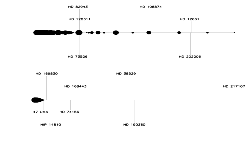
Figure 1.— Effective distance from mean motion resonance for all known pairs of planets in two-planet multiplanet systems, measured in semimajor axis ratio. Locations of 1st, 2nd, 3rd, 4th, 5th and 6th order mean motion resonances are given by dots of decreasing size. The lower horizontal line is on a broader scale than the top line.

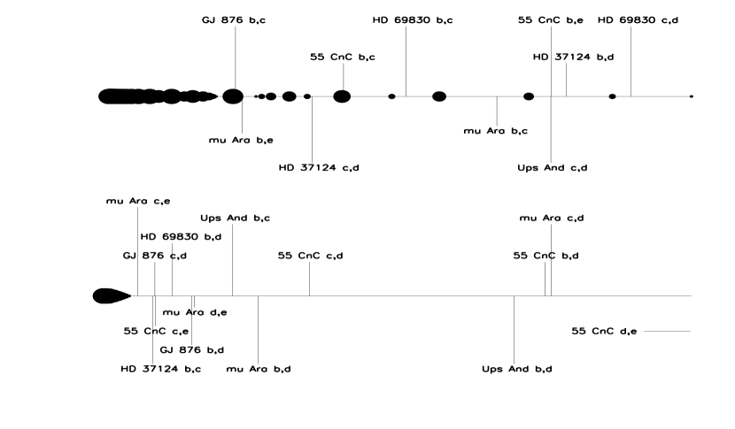
Figure 2.— Effective distance from mean motion resonance for all known pairs of planets in multiplanet systems with more than two planets, measured in semimajor axis ratio. Locations of 1st, 2nd, 3rd, 4th, 5th and 6th order mean motion resonances are given by dots of decreasing size. The lower horizontal line is on a broader scale than the top line.

6. Application to known exosystems

6.1. Overview

Extrasolar planet data is updated constantly, and the resulting orbital solutions are bound to change with the passage of time. Nevertheless, in many cases the errors on currently known orbital parameters allow one to achieve a representative qualitative description of the motion, and often a highly accurate quantitative solution as well. In order to help determine which extrasolar planets are dominated by secular perturbations instead of mean motion resonances (MMRs), we compute the “effective distance” away from a strong MMR for each pair of planets. The “nominal” (approximate) locations of MMRs are given by $[(p+n)/p]^{-(2/3)}$, where $n$ represents the order of the resonance and $p$ is an integer. Therefore, a scale-free method of representing this “effective distance” from resonance is to use this quantity as the metric (Champenois & Vienne, 1999). Figures 1-2 provide a summary of our current (as of Jan. 1, 2007) understanding of all known multiple-planet extrasolar systems. A schematic of the effective distance from resonance is provided for all two-planet systems (Fig. 1) and all known systems with more than two planets (Fig. 2). Table 1 lists the relevant orbital parameters for the systems simulated in this study. We deem these systems to be sufficiently far from any MMR, and hence “secular”. All orbital parameters are taken from Jean Schneider’s Extrasolar Planets Encyclopedia, and for all data we take $\sin{i}$ to be unity. All N-body numerical integrations are carried out with the Bulirsch-Stoer HNbody integrator (K.P. Rauch & D. P. Hamilton 2007, in preparation).

Table 1?-PLANET EXTRASOLAR SYSTEMS

Planet	$m$ ($m_{Jup}$)	$m_{\ast}$ ($m_{\odot}$)	$a$ (AU)	$e$	$\varpi$ (deg)
HD 12661 b	2.30		0.83	0.35	291.73
HD 12661 c	1.57	1.07	2.56	0.2	162.4
HD 38529 b	0.78		0.129	0.29	87.7
HD 38529 c	12.7	1.39	3.68	0.36	14.7
HD 168443 b	8.02		0.30	0.5286	172.87
HD 168443 c	18.1	0.96	3.91	0.2125	65.07
HD 108874 b	1.36		1.051	0.07	248.4
HD 108874 c	1.018	1.00	2.68	0.25	17.3
$\upsilon$ And b	0.690		0.0590	0.029	46.0
$\upsilon$ And c	1.98	1.30	0.830	0.254	232.4
$\upsilon$ And d	3.95		2.51	0.242	258.5

Table 2 Summary of masses, semimajor axes, eccentricities and longitude of pericenters for the multi-planet extrasolar systems studied here. These parameters were taken from Jean Schneider’s Extrasolar Planets Encyclopedia with $\sin{i}$ assumed to be unity.

We study only those planets which satisfy a particular constraint regarding Kaula’s (1961; 1962) expansion of the disturbing function, which is based on Laplace coefficients. Sundman (1916) determined that in the planar form of this expansion, Laplace coefficients are sure to converge only if the following criterion is satisfied (Ferraz-Mello, 1994; S̆idlichovský & Nesvorný, 1994):

$$a_{2}H(e_{2})<a_{1}h(e_{1}),$$ (35)

where

$$H(q) =\sqrt{1+q^{2}}\cosh{w}+q+\sinh{w},$$ (36)

$$h(q) =\sqrt{1+q^{2}}\cosh{w}-q-\sinh{w},$$ (37)

such that $w$ is implicitly defined as $w=q\cosh{w}$. We applied this test to each pair of planets in the same system; failing this test implies that the use of LL theory, or any other theory relying on Laplace coefficients, is suspect. Therefore, we only consider pairs of planets which pass this test.

6.2. Systems with two planets

6.2.1 HD 12661

Lee & Peale (2003) use octupole-level secular theory and Rodríguez & Gallardo (2005) use a sixth-order expansion of Kaula’s disturbing function in order to study the planets orbiting HD 12661, and conclude that the system is strongly dominated by secular motions. However, older work indicated that the system might be trapped in a $6$:$1$ (Goździewski & Maciejewski, 2003) resonance or is on the border of a $11$:$2$ (Goździewski, 2003) MMR.

We seek to determine how well the traditional and generalized versions of LL theory reproduce motion in HD 12661, and further compare these methods with octupole-level secular theory. Figs. 3-4 explore the dynamical state of the system, and demonstrate that none of the theories employed here model the true evolution well. Considering first the variation of the eccentricity of $e_{1}$, the fourth-order LL theory matches best the secular periodicity, eccentricity amplitude, and eccentricity values of the profile exhibited by the true evolution. Octupole theory matches fourth-order LL theory in their predictions for the lower bounds of the eccentricity of both planets, and both theories represent a significant improvement over traditional LL theory with regard to eccentricity amplitude. All theories and the actual dynamical evolution exhibit apsidal libration with a $\approx 60^{\circ}$ amplitude. Overall, the profiles and periodicities of the apsidal libration for both the fourth-order LL theory and octupole theory improve upon the traditional theory, with the frequency from the fourth-order LL theory mirroring the actual evolution best but still not well.

Figure 3.— Eccentricity and apsidal angle variation according to the traditional LL theory (solid lines in the lower two panels and leading dark loops in the uppermost panel), the fourth-order LL theory (dotted lines in the lower two panels and light loops in the uppermost panel), and octupole-level secular perturbation theory (dashed lines in the lower two panels and trailing dark loops in the uppermost panel) for the HD 12661 system.

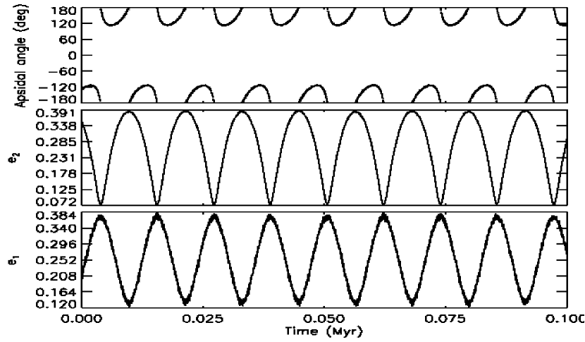
Figure 4.— Eccentricity and apsidal angle variation from an N-body simulation for the HD 12661 system.

6.2.2 HD 168443

Although the HD 168443 system (Marcy et al., 2001) is thought to harbor a brown dwarf (Udry et al., 2002; Reffert & Quirrenbach, 2006), Érdi et al. (2004) investigate the dynamical structure of a possible habitable zone in the system. Even though HD 168443 b has a large eccentricity ($e_{2}\approx 0.53$), the wide separation of both planets allows the Sundman inequality to be satisfied. This same eccentricity, however, produces a significant difference in the dynamical predictions from the second- and fourth-order LL theories (Fig. 5). Both the fourth-order LL theory and the octupole theory reproduce the eccentricity values and amplitude of both planets well, even including the short-period variations in the true evolution of $e_{1}$ (Fig. 6). Despite this good agreement, over the course of just $10^{5}$ yr, the frequency of the eccentricity variation drifts by about half of a period. The circulating apsidal angle observed in the true evolution has an additional small-period noisy variation which encompasses both the profiles from the fourth-order LL theory and the octupole-level theory over $10^{5}$ yr.

Figure 5.— Eccentricity and apsidal angle variation according to the traditional LL theory (solid lines in the lower two panels and light squares in the uppermost panel), the fourth-order LL theory (dotted lines in the lower two panels and dots in the uppermost panel), and octupole-level secular perturbation theory (dashed lines in the lower two panels and thick triangles in the uppermost panel) for the HD 168443 system.

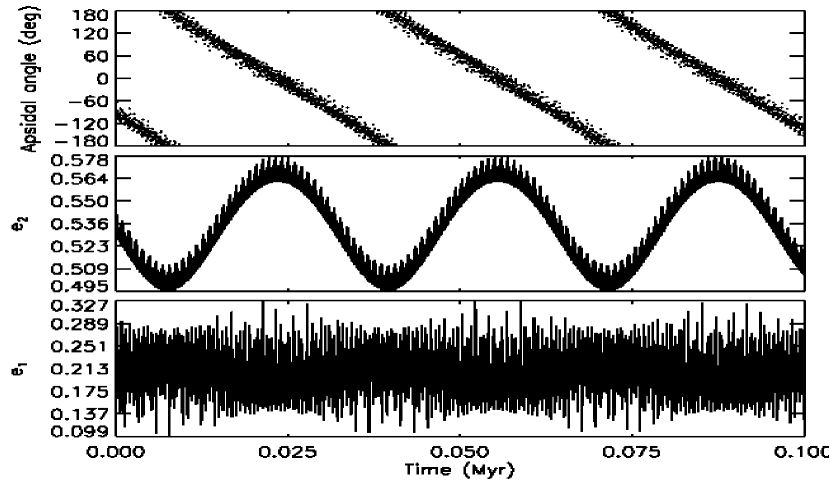
Figure 6.— Eccentricity and apsidal angle variation from an N-body simulation for the HD 168443 system.

Figure 7.— Eccentricity and apsidal angle variation according to the traditional LL theory (solid lines in the lower two panels and light squares in the uppermost panel), the fourth-order LL theory (dotted lines in the lower two panels and dots in the uppermost panel), and octupole-level secular perturbation theory (dashed lines in lower two panels and thick triangles in the uppermost panel) for the HD 38529 system.

Figure 8.— Eccentricity and apsidal angle variation from an N-body simulation for the HD 38529 system.

Figure 9.— Eccentricity and apsidal angle variation according to the traditional LL theory (solid lines in the lower two panels and light squares in the uppermost panel), the fourth-order LL theory (dotted lines in the lower two panels and dots in the uppermost panel), and octupole-level secular perturbation theory (dashed lines in the lower two panels and thick triangles in the uppermost panel) for the planet pair $\upsilon$ And c and $\upsilon$ And d.

Figure 10.— Eccentricity and apsidal angle variation from an N-body simulation for the planet pair $\upsilon$ And c and $\upsilon$ And d.

6.2.3 HD 38529

The HD 38529 system has been studied in the same context as the HD 168443 system, as both contain a planet which could be a brown dwarf. In HD 38429, however, the eccentricity of the more massive, outer, planet exceeds that of the inner planet. The result of this different configuration is that octupole theory matches the true evolution better than fourth-order LL theory, as can be seen in Figs. 7-8. The agreement achieved in the eccentricity values and amplitudes of the inner planet is particularly good (within 1%) between the octupole theory and the true evolution. The eccentricity amplitude achieved by the fourth-order LL theory is actually worse than that from the traditional theory, although the secular frequency is better modeled by the fourth-order theory. The long ($>5\times 10^{4}$ yr) circulation period of the apsidal angle differs from that predicted by the fourth-order LL theory and octupole theory by only a few percent.

Despite some positive agreement, no theory varies the outer planet’s eccentricity by more than $0.0003$, and this eccentricity is centered nearly around $e_{2}=0.3600$. Both these characteristics starkly display the inadequacy of any of these theories to quantitatively describe the admittedly minor but non-negligible perturbations by the less massive inner planet on the more massive moderately eccentric outer one.

6.3. Systems with more than two planets

Although one pair of planets in a multi-planet system may reside in a mean motion resonance, other pairs of planets in the system may evolve primarily by secular means. In three-planet systems with a MMR between two of the planets, the other planet’s evolution will be affected, albeit indirectly, by non-secular motions. Strong (1st, 2nd, or 3rd order) MMRs are likely to significantly influence the $\mu$ Ara, GJ 876, and $55$ Cnc systems, and planets in the $55$ Cnc, GJ 876, $\upsilon$ And, and HD 69830 systems are all close enough ($a<0.07$ AU) to their parent stars to have been tidally influenced, possibly resulting in a reduction of their eccentricities. Further, a pair of planets in the HD 37124 system fail to satisfy the Sundman Criterion for convergence of Laplace coefficients in terms of the disturbing function. All these observations cast doubt on the effective use of LL secular theory, even a generalized N-body version, on the majority of the currently known three and four-planet extrasolar planetary systems. One exception is provided by Ji et al. (2006), who demonstrate that the orbital evolution of the three planets in the HD 69830 are well-described with LL secular theory due to their small eccentricities and relatively large orbital separations.

Despite these reservations, one may apply LL theory to the planet pair $\upsilon$ And c and $\upsilon$ And d. The results, presented in Figs. 9-11, perhaps showcase best how even the fourth-order theory can fail. Both the traditional LL theory and the fourth-order theory predict circulation of the apsidal angle, whereas only the octupole theory instead correctly predicts apsidal libration. This key distinction casts doubt on the ability of fourth-order LL theory to make reliable qualitative or quantitative predictions for multi-planet extrasolar systems in general.

Still, such systems may demonstrate the variety of phase space portraits allowed by the theory. Figure 11 displays a panorama of regions in eccentricity phase space in which apsidal libration is allowed according to traditional LL theory and fourth-order LL theory. The figure hints at the branch point introduced by the discriminant in Eq. (25), and demonstrates that traditional LL theory overestimates the region of phase space which allows for apsidal libration to occur. This dense and varied phase portrait demonstrates how strongly the fourth-order modification to traditional LL theory may play a role in an extrasolar system.

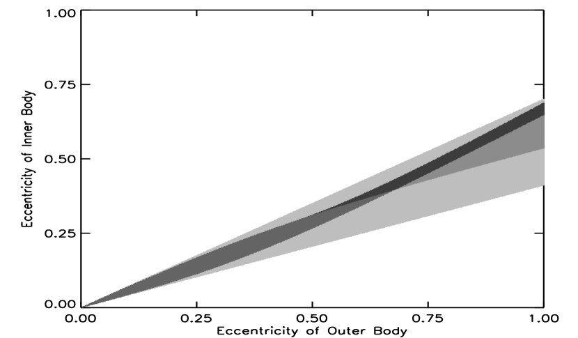
Figure 11.— Regions of the $\upsilon$ And c - $\upsilon$ And d eccentricity phase space which allow for libration from the traditional LL theory only (light gray), traditional LL theory and the generalized LL theory for the lower sign from Eq. (25) only (medium gray), traditional LL theory and the generalized LL theory for the upper sign from Eq. (25) only (dark gray), and the traditional LL theory and both branches of the generalized LL theory (black).

7. Discussion

Our demonstration of LL theory’s limitations for extrasolar planetary motions of known systems should not overshadow its utility in modeling other dynamical systems, including Solar System analogs. Although MMRs help establish the framework of planetary systems (Gomes et al., 2005; Morbidelli et al., 2005; Tsiganis et al., 2005), their final states might be dominated by purely secular perturbations (Brouwer & van Woerkom, 1950; Laskar, 1988; Ito & Tanikawa, 2002). Quantitatively accurate secular solutions are difficult to obtain, even on a $\sim 1-100$ Myr timescale, as both stable and chaotic long-term ($\gtrsim 1$ Gyr) solutions exist for the Solar System within the uncertainties of current measurements (Hayes, 2006). Therefore, analytical results such as those from Eqs. (18)-(21), (22) and (31)-(33) may give representative qualitative descriptions of the dynamical state of the system on timescales shorter than those which may give rise to destructive stochasticity.

A purely secular theory, by definition, does not incorporate the effects from the resonant terms which may cause the theory to fail. The true disturbing function includes an infinite number of terms, and depending on the orbital parameters of both resonant bodies, each term containing mean longitudes has a particular “strength”. In essence, a secular theory eliminates all of these terms, and justifies this neglect by appealing to how the combined strength of these terms should not match the strength of those terms without mean longitudes. In reality, however, resonant terms play a non-negligible role in the evolution of seemingly secular planetary and satellite systems.

Malhotra et al. (1989) presented a way to incorporate “near-resonant” terms into Laplace-Lagrange secular theory, significantly improving their results. A similar approach could be invoked for fourth-order LL theory in order to improve its current general lack of agreement with the actual evolution of multi-planet exosystems. If the strong “near-resonant” term in question is a low-order resonance, then only one or two resonant terms might significantly impact the motion. With assumptions about the period of these terms, their tendency to circulate instead of librate at near-commensurabilities, the constancy of their coefficients, and their decoupled states, one can model each term as a pendulum, the paradigm for single-resonance models. The pendulum model allows one to define an energy and compute a circulation period for each resonant term, and ultimately to include the relevant averaged effects into the disturbing function. Malhotra et al. (1989) perform this task for first-order near-resonances. As per their discussion, expanding their theory in order to encompass a treatment such as ours would involve deriving the corrections due to second-order near-resonances and possibly dealing with the corrections introduced from coupling between resonant terms.

Because secular eigenfrequencies are proportional to the resonant mass/central mass ratio and to the mean motion of the resonant masses, the utility of LL theory largely hinges on the values of the masses and semimajor axes of the resonant objects. Unlike for secular satellite systems (Malhotra et al., 1989; Christou & Murray, 1997), the mass ratio in extrasolar systems is orders of magnitude larger. The result is that the quality of the results obtained from LL theory is sensitive to this ratio, a result also suggested by our numerical investigations. The planets in HD 108873 are close to a $4$:$1$ MMR. Using the parameters for the planets from Table 1, we find that the system’s properties are sensitively dependent on the exoplanet masses and semimajor axis ratio, but are more robust to changes in initial eccentricity. A possible (but speculative) reason for this characterization is that eccentricities appear in the expressions for coefficients of resonant terms, but are not included in the expressions for the secular eignefrequencies.

The neglect of inclination in our fourth-order theory – although already justified by the 1) unknown inclinations of the vast majority of extrasolar planets, 2) near-coplanarity of several dynamical subsystems in the Solar System, and 3) complexities arising from the coupling of eccentricity and inclination in fourth-order LL theory – may not be of significant consequence given the marginal improvement afforded by expanding the theory to include eccentricity terms up to fourth-order. However, such coupled terms might introduce important nonlinearities in the solution of LL theory for fully three-dimensional problems, and deserve consideration in future studies.

A subsequent planar expansion to arbitrary order is possible and may proceed along the same lines as the method outlined here. Expansion to $N$th order will involve terms in the disturbing function of the form $\cos{\left[N\left(\varpi_{l}-\varpi_{p}\right)\right]}$, which can be expressed as polynomials in $\cos{\varpi_{l}}$ and $\cos{\varpi_{p}}$. The differential equations representing the motion will contain $h_{j}$, $h_{k}$, $k_{j}$ and $k_{k}$ terms of all odd orders up to $\left(N-1\right)$th order. However, such an expansion may only be useful when seeking a highly accurate solution in systems where effects from barycentric drifts, short-period terms and MMRs may all be safely neglected.

One may also generalize LL theory to fourth-order in the inclinations but not the eccentricities when modeling inclined circular orbits. Under the small angle approximation, $\sin{I_{j}/2}\approx I_{j}/2$, where $I_{j}$ is the inclination of body $j$, the equations of motions and criteria for nodal libration will have exactly the same form as those of the planar case, except that the constants will not depend on the relative locations of the bodies being perturbed (i.e. no delta functions would appear in the analog of Eq. 27) as there is no preferred reference plane. A consequence is that the nodal rate of an inclined massless particle interior to a giant planet on a circular coplanar orbit would remain unchanged if the bodies switched semimajor axes. To fourth order, this rate would be dependent on the massless particle’s inclination, and be equal to:

$$C_{a}^{(j)}\left[\left(\frac{1}{4}\right)2f_{3}+\bigg{\{}\left(\frac{1}{16}\right)4f_{8}-\left(\frac{1}{4}\right)f_{3}\bigg{\}}I_{j}^{2}\right]$$

$$\approx C_{a}^{(j)}\bigg{[}-\frac{3}{4}\alpha\left(1-\frac{1}{2}I_{j}^{2}\right)+\frac{153}{128}\alpha^{2}I_{j}^{2}$$ (38)

$$-\frac{45}{32}\alpha^{3}\left(1-\frac{1}{2}I_{j}^{2}\right)+\mathcal{O}\left(\alpha^{4}\right)\bigg{]}$$

Comparison with Eq. (21) demonstrates a difference of sign, but a remarkable similarity of coefficients. In fact, reduction to the traditional LL theory and to second order in $\alpha$ demonstrates that the nodal rate exceeds the apsidal rate by exactly a factor of $\alpha$. The differences in the presence of powers of $\alpha$ in Eqs. (21) and (38) are due to the different functions of the Laplace coefficients which arise naturally from the expansion of Kaula’s disturbing function about zero eccentricities and inclinations.

8. Conclusion

We have presented an analytical planar fourth-order (in eccentricity) formulation of traditional Laplace-Lagrange theory for two non-central bodies (Eqs. 14-15 and A1a-A1h) and for $N$ non-central bodies (Eqs. 28-29 and A2a-A2j), and derived conditions for apsidal libration in various cases (Eqs. 23-26 and 31-34). We have surveyed the prospects for secular resonance in multi-planet extrasolar systems, and, where appropriate, applied the traditional and generalized versions of LL theory and octupole-level theory to the systems. We conclude that expansion to high-eccentricity orders fails to compensate for the inherent drawbacks of the traditional theory when applied to extrasolar planetary systems, and is best utilized in dynamical systems with more restrictive orbital parameters.

Figure 12.— Percent error incurred when using the series expansion in $\alpha$ of $f_{i}$ quantities (in Eqs. B13-B22) relative to the exact computation for $f_{2}$ (solid line), $f_{4}$ (dotted line), $f_{5}$ (dashed line), $f_{6}$ (dash-dot line), and $f_{10}$ (dash-dot-dot-dot line) for the $\alpha$ given from HD 12661.

Appendix A Appendix A

The following constants in time, expressed as functions of the planetary semimajor axes and masses only, are used in the two-body fourth-order LL theory from Eq. (15):

$$C_{a}^{(1)}\equiv\mathcal{G}a_{1}^{-\frac{3}{2}}m_{2}\mu_{1}^{-\frac{1}{2}}\quad\quad C_{a}^{(2)}\equiv\mathcal{G}a_{1}^{-1}a_{2}^{-\frac{1}{2}}m_{1}\mu_{2}^{-\frac{1}{2}}$$ (A1a)

$$C_{1}\equiv 2f_{2}\quad\quad C_{2}\equiv f_{10}$$ (A1b)

$$C_{3}^{(1)}\equiv 4f_{6}-f_{2}\quad\quad C_{3}^{(2)}\equiv 4f_{4}-f_{2}$$ (A1c)

$$C_{4}\equiv 2f_{5}-2f_{17}\quad\quad C_{5}\equiv 2f_{5}+2f_{17}$$ (A1d)

$$C_{6}^{(1)}\equiv 3f_{12}-\frac{1}{2}f_{10}\quad\quad C_{6}^{(2)}\equiv 3f_{11}-\frac{1}{2}f_{10}$$ (A1e)

$$C_{7}^{(1)}\equiv f_{12}\quad\quad C_{7}^{(2)}\equiv f_{11}$$ (A1f)

$$C_{8}^{(1)}\equiv 2f_{12}\quad\quad C_{8}^{(2)}\equiv 2f_{11}$$ (A1g)

$$C_{9}\equiv 4f_{17}$$ (A1h)

The following constants are a modified, more general, form of those in Eqs. (A1a)-(A1h), used in the N-body fourth-order LL theory from Eq. (29):

$$C_{a}^{(lp)} \equiv \mathcal{G}a_{j}^{-\frac{1}{2}}a_{l}^{-\frac{1}{2}}m_{k}\mu_{j}^{-\frac{1}{2}}$$ (A2a)

$$C_{1}^{(lp)} \equiv 2f_{2}^{(lp)}$$ (A2b)

$$C_{2}^{(lp)} \equiv f_{10}^{(lp)}$$ (A2c)

$$C_{3}^{(lp)} \equiv 4\left[\delta\left(j-p\right)f_{4}^{(lp)}+\delta\left(j-l\right)f_{6}^{(lp)}\right]-f_{2}^{(lp)}$$ (A2d)

$$C_{4}^{(lp)} \equiv 2f_{5}^{(lp)}-2f_{17}^{(lp)}$$ (A2e)

$$C_{5}^{(lp)} \equiv 2f_{5}^{(lp)}+2f_{17}^{(lp)}$$ (A2f)

$$C_{6}^{(lp)} \equiv 3\left[\delta\left(j-p\right)f_{11}^{(lp)}+\delta\left(j-l\right)f_{12}^{(lp)}\right]-\frac{1}{2}f_{10}^{(lp)}$$ (A2g)

$$C_{7}^{(lp)} \equiv \delta\left(j-p\right)f_{11}^{(lp)}+\delta\left(j-l\right)f_{12}^{(lp)}$$ (A2h)

$$C_{8}^{(lp)} \equiv 2\left[\delta\left(j-p\right)f_{11}^{(lp)}+\delta\left(j-l\right)f_{12}^{(lp)}\right]$$ (A2i)

$$C_{9}^{(lp)} \equiv 4f_{17}^{(lp)}$$ (A2j)

Appendix B Appendix B

One may express constants found in the coefficients of terms in the disturbing function as functions of derivatives of Laplace coefficients. From Murray & Dermott (1999), secular dynamics yield the following forms:

$$f_{2} = \frac{1}{4}\alpha\mathcal{D}b_{\frac{1}{2}}^{(0)}\left(\alpha\right)+\frac{1}{8}\alpha^{2}\mathcal{D}^{2}b_{\frac{1}{2}}^{(0)}\left(\alpha\right)$$ (B1a)

$$f_{3} = -\frac{1}{4}\alpha b_{\frac{3}{2}}^{(-1)}\left(\alpha\right)-\frac{1}{4}\alpha b_{\frac{3}{2}}^{(1)}\left(\alpha\right)$$ (B1b)

$$f_{4} = \frac{1}{32}\alpha^{3}\mathcal{D}^{3}b_{\frac{1}{2}}^{(0)}\left(\alpha\right)+\frac{1}{128}\alpha^{4}\mathcal{D}^{4}b_{\frac{1}{2}}^{(0)}\left(\alpha\right)$$ (B1c)

$$f_{5} = \frac{1}{8}\alpha\mathcal{D}b_{\frac{1}{2}}^{(0)}\left(\alpha\right)+\frac{7}{16}\alpha^{2}\mathcal{D}^{2}b_{\frac{1}{2}}^{(0)}\left(\alpha\right)+\frac{1}{4}\alpha^{3}\mathcal{D}^{3}b_{\frac{1}{2}}^{(0)}\left(\alpha\right)+\frac{1}{32}\alpha^{4}\mathcal{D}^{4}b_{\frac{1}{2}}^{(0)}\left(\alpha\right)$$ (B1d)

$$f_{6} = \frac{3}{16}\alpha\mathcal{D}b_{\frac{1}{2}}^{(0)}\left(\alpha\right)+\frac{9}{32}\alpha^{2}\mathcal{D}^{2}b_{\frac{1}{2}}^{(0)}\left(\alpha\right)+\frac{3}{32}\alpha^{3}\mathcal{D}^{3}b_{\frac{1}{2}}^{(0)}\left(\alpha\right)+\frac{1}{128}\alpha^{4}\mathcal{D}^{4}b_{\frac{1}{2}}^{(0)}\left(\alpha\right)$$ (B1e)

$$f_{8} = \frac{3}{16}\alpha^{2}b_{\frac{5}{2}}^{(-2)}\left(\alpha\right)+\frac{3}{4}\alpha^{2}b_{\frac{5}{2}}^{(0)}\left(\alpha\right)+\frac{3}{16}\alpha^{2}b_{\frac{5}{2}}^{(2)}\left(\alpha\right)$$ (B1f)

$$f_{10} = \frac{1}{2}b_{\frac{1}{2}}^{(1)}\left(\alpha\right)-\frac{1}{2}\alpha\mathcal{D}b_{\frac{1}{2}}^{(1)}\left(\alpha\right)-\frac{1}{4}\alpha^{2}\mathcal{D}^{2}b_{\frac{1}{2}}^{(1)}\left(\alpha\right)$$ (B1g)

$$f_{11} = -\frac{1}{8}\alpha^{2}\mathcal{D}^{2}b_{\frac{1}{2}}^{(1)}\left(\alpha\right)-\frac{3}{16}\alpha^{3}\mathcal{D}^{3}b_{\frac{1}{2}}^{(1)}\left(\alpha\right)-\frac{1}{32}\alpha^{4}\mathcal{D}^{4}b_{\frac{1}{2}}^{(1)}\left(\alpha\right)$$ (B1h)

$$f_{12} = \frac{1}{8}b_{\frac{1}{2}}^{(1)}\left(\alpha\right)-\frac{1}{8}\alpha\mathcal{D}b_{\frac{1}{2}}^{(1)}\left(\alpha\right)-\frac{11}{16}\alpha^{2}\mathcal{D}^{2}b_{\frac{1}{2}}^{(1)}\left(\alpha\right)$$ (B1i)

$$- \frac{5}{16}\alpha^{3}\mathcal{D}^{3}b_{\frac{1}{2}}^{(1)}\left(\alpha\right)-\frac{1}{32}\alpha^{4}\mathcal{D}^{4}b_{\frac{1}{2}}^{(1)}\left(\alpha\right)$$ (B1j)

$$f_{17} = \frac{3}{16}b_{\frac{1}{2}}^{(2)}\left(\alpha\right)-\frac{3}{16}\alpha\mathcal{D}b_{\frac{1}{2}}^{(2)}\left(\alpha\right)+\frac{3}{32}\alpha^{2}\mathcal{D}^{2}b_{\frac{1}{2}}^{(2)}\left(\alpha\right)$$ (B1k)

$$+ \frac{1}{8}\alpha^{3}\mathcal{D}^{3}b_{\frac{1}{2}}^{(2)}\left(\alpha\right)+\frac{1}{64}\alpha^{4}\mathcal{D}^{4}b_{\frac{1}{2}}^{(2)}\left(\alpha\right)$$ (B1l)

where $b_{\frac{1}{2}}^{(0)}$ is a Laplace coefficient and $\mathcal{D}$ is a differential operator. Using the hypergeometric expansion of the Laplace coefficients (Murray & Dermott, 1999) one may show that:

$$f_{2} = \frac{3}{8}\alpha^{2}+\frac{45}{64}\alpha^{4}+\frac{525}{512}\alpha^{6}+\frac{11025}{8192}\alpha^{8}+\frac{218295}{131072}\alpha^{10}+\frac{2081079}{1048576}\alpha^{12}$$ (B2a)

$$f_{3} = -\frac{3}{2}\alpha^{2}-\frac{45}{16}\alpha^{4}-\frac{525}{128}\alpha^{6}-\frac{11025}{2048}\alpha^{8}-\frac{218295}{32768}\alpha^{10}-\frac{2081079}{262144}\alpha^{12}$$ (B2b)

$$f_{4} = \frac{135}{512}\alpha^{4}+\frac{2625}{2048}\alpha^{6}+\frac{231525}{65536}\alpha^{8}+\frac{1964655}{262144}\alpha^{10}+\frac{114459345}{8388608}\alpha^{12}$$ (B2c)

$$f_{5} = \frac{9}{16}\alpha^{2}+\frac{225}{64}\alpha^{4}+\frac{11025}{1024}\alpha^{6}+\frac{99225}{4096}\alpha^{8}+\frac{12006225}{262144}\alpha^{10}+\frac{81162081}{1048576}\alpha^{12}$$ (B2d)

$$f_{6} = \frac{15}{32}\alpha^{2}+\frac{945}{512}\alpha^{4}+\frac{4725}{1024}\alpha^{6}+\frac{606375}{65536}\alpha^{8}+\frac{8513505}{524288}\alpha^{10}+\frac{218513295}{8388608}\alpha^{12}$$ (B2e)

$$f_{8} = \frac{3}{2}\alpha^{2}+\frac{405}{32}\alpha^{4}+\frac{2625}{64}\alpha^{6}+\frac{385875}{4096}\alpha^{8}+\frac{5893965}{32768}\alpha^{10}+\frac{160243083}{524288}\alpha^{12}$$ (B2f)

$$f_{10} = -\frac{15}{16}\alpha^{3}-\frac{105}{64}\alpha^{5}-\frac{4725}{2048}\alpha^{7}-\frac{24255}{8192}\alpha^{9}-\frac{945945}{262144}\alpha^{11}$$ (B2g)

$$f_{11} = -\frac{45}{64}\alpha^{3}-\frac{525}{128}\alpha^{5}-\frac{99225}{8129}\alpha^{7}-\frac{218295}{8192}\alpha^{9}-\frac{52026975}{1048576}\alpha^{11}$$ (B2h)

$$f_{12} = -\frac{75}{32}\alpha^{3}-\frac{2205}{256}\alpha^{5}-\frac{42525}{2048}\alpha^{7}-\frac{1334025}{32768}\alpha^{9}-\frac{36891855}{524288}\alpha^{11}$$ (B2i)

$$f_{17} = \frac{315}{256}\alpha^{4}+\frac{4725}{1024}\alpha^{6}+\frac{363825}{32768}\alpha^{8}+\frac{2837835}{131072}\alpha^{10}+\frac{156080925}{4194304}\alpha^{12}$$ (B2j)

Importantly, in the computation of derivatives of Laplacian coefficients with negative $j$ values, the absolute value of $j$ must be taken before the application of recurrence derivative formulas such as those from Eqs. (6.70)-(6.71) of Murray & Dermott (1999). Fig. 12 demonstrates the error incurred by truncating some of the above expansions to various powers of $\alpha$ for $\alpha\approx 0.32$, the value for the planets in the HD 12661 system.

Appendix C Appendix C

Here we express the auxiliary variables from Eq. (34) as time-dependent functions of eccentricities, semimajor axis ratios, and terrestrial planet-giant planet mass ratio for a giant planet residing in between (case 1), exterior to (case 2), or interior to (case 3) two terrestrial planets. For case 1:

$$Q^{(13)} = \mathcal{M}C_{2}^{(13)}\alpha_{12}\left(\sqrt{\alpha_{13}}-1\right)e_{1}e_{3}-2C_{2}^{(23)}e_{2}e_{3}\cos{\left(\varpi_{1}-\varpi_{2}\right)}$$ (C1)

$$S^{(13)} = 2C_{2}^{(23)}e_{2}e_{3}\sin{\left(\varpi_{1}-\varpi_{2}\right)}$$ (C2)

$$R^{(13)} = 2\left(\alpha_{12}\sqrt{\alpha_{13}}\frac{C_{1}^{(12)}}{2}e_{1}^{2}-\frac{C_{1}^{(23)}}{2}e_{3}^{2}+\alpha_{12}\sqrt{\alpha_{13}}C_{2}^{(12)}e_{1}e_{2}\cos{\left(\varpi_{1}-\varpi_{2}\right)}\right)$$ (C3)

For Case 2:

$$Q^{(23)} = \mathcal{M}C_{2}^{(23)}\frac{\left(\sqrt{\alpha_{23}}-1\right)}{\alpha_{12}}e_{2}e_{3}-2C_{2}^{(13)}e_{1}e_{3}\cos{\left(\varpi_{1}-\varpi_{2}\right)}$$ (C4)

$$S^{(23)} = -2C_{2}^{(13)}e_{1}e_{3}\sin{\left(\varpi_{1}-\varpi_{2}\right)}$$ (C5)

$$R^{(23)} = 2\left(\frac{\sqrt{\alpha_{23}}}{\alpha_{12}}\frac{C_{1}^{(12)}}{2}e_{2}^{2}-\frac{C_{1}^{(13)}}{2}e_{3}^{2}+\frac{\sqrt{\alpha_{23}}}{\alpha_{12}}C_{2}^{(12)}e_{1}e_{2}\cos{\left(\varpi_{1}-\varpi_{2}\right)}\right)$$ (C6)

For Case 3:

$$Q^{(12)} = \mathcal{M}C_{2}^{(12)}\alpha_{12}\left(\sqrt{\alpha_{12}}-1\right)e_{1}e_{2}-2C_{2}^{(23)}e_{2}e_{3}\cos{\left(\varpi_{1}-\varpi_{3}\right)}$$ (C7)

$$S^{(12)} = 2C_{2}^{(23)}e_{2}e_{3}\sin{\left(\varpi_{1}-\varpi_{3}\right)}$$ (C8)

$$R^{(12)} = 2\left(\alpha_{12}\sqrt{\alpha_{12}}\frac{C_{1}^{(13)}}{2}e_{1}^{2}-\frac{C_{1}^{(23)}}{2}e_{2}^{2}+\alpha_{12}\sqrt{\alpha_{12}}C_{2}^{(13)}e_{1}e_{3}\cos{\left(\varpi_{1}-\varpi_{3}\right)}\right)$$ (C9)

References

• Adams & Laughlin (2006) Adams, F.C., Laughlin, G. 2006 ApJ, 649, 992
• Artymowicz et al. (1991) Artymowicz, P., Clarke, C. J., Lubow, S. H., & Pringle, J. E. 1991 ApJ, 370, L35
• Barnes & Greenberg (2006) Barnes, R., Greenberg, R. 2006 ApJ, 638, 478
• Beaugé, Ferraz-Mello & Michtchenko (2003) Beaugé, C., Ferraz-Mello, S., Michtchenko, T.A. 2003 ApJ, 593, 1124
• Beaugé, Nesvorný, & Dones (2006) Beaugé, C., Nesvorný, D., Dones, L. 2006 AJ, 131, 2299
• Breiter (1999) Breiter, S.Ł 1999 CeMDA, 74, 253
• Brouwer & van Woerkom (1950) Brouwer, D., & van Woerkom, A.J.J. 1950 Astron. P. Amer. Ephem., 13, 81
• Brouwer & Clemence (1961) Brouwer, D., & Clemence, G. 1961, Methods of Celestial Mechanics (New York: Acadmic Press)
• Butler et al. (1997) Butler, R.P., Marcy, G.W., Williams, E., Hauser, H., Shirts, P. 1997 ApJ, 474, L115
• Butler et al. (2006) Butler, R.P., Wright, J.T., Marcy, G.W., Fischer, D.A., Vogt, S.S., Tinney, C.G., Jones, H.R.A., Carter, B.D., Johnson, J.A., McCarthy C., Penny, A.J. 2006 ApJ, 646, 505
• Champenois & Vienne (1999) Champenois, S., Vienne, A. 1999 CeMDA, 74, 111
• Charbonneau (2006) Charbonneau, D. 2006 Nature, 441, 292
• Chiang & Murray (2002) Chiang, E.I, Murray, N. 2002 ApJ, 576, 473
• Christou & Murray (1997) Christou, A.A., Murray, C.D. 1997 A&A 327, 416
• Ćuk & Burns (2004) Ćuk, M., Burns, J.A. 2004 AJ, 128, 2518
• Ellis & Murray (2000) Ellis, K.M., Murray, C.D. 2000 Icarus, 147, 129
• Érdi et al. (2004) Érdi, B., Dvorak, R., Sándor, Z., Pilat-Lohinger, E., Funk, B. 2004 MNRAS, 351, 1043
• Féjoz (2002) Féjoz, J. 2002 CeMDA, 84, 159
• Ferraz-Mello (1994) Ferraz-Mello, S. 1994 AJ, 96, 400
• Ford, Kozinsky & Rasio (2000) Ford, E.B., Kozinsky, B., Rasio, F.A. 2000 ApJ 535, 385
• Ford, Lystad & Rasio (2005) Ford, E. B., Lystad, V., Rasio, F. A. 2005, Nature, 434, 873
• Ford, Rasio & Yu (2003) Ford, E. B., Rasio, F. A., & Yu, K. 2003, in “Scientific Frontiers in Research on Extrasolar Planets”, ASP Conf. Ser. Vol 294, eds D. Deming and S. Seager (San Francisco: ASP), p. 181
• Gladman (1993) Gladman, B. 1993 Icarus, 106, 247
• Goldreich & Sari (2003) Goldreich, P., & Sari, R. 2003, ApJ, 585, 1024
• Gomes et al. (2005) Gomes, R., Levison, H.F., Tsiganis, K, Morbidelli, A. 2005 Nature 435, 466
• Goździewski (2003) Goździewski, K. 2003 A&A, 398, 1151
• Goździewski & Maciejewski (2003) Goździewski, K., Maciejewski, A. J. 2003 ApJL, 586, L153
• Greenberg (1977) Greenberg, R. 1977 VA, 21, 209
• Hayes (2006) Hayes, W. DDA 2006 meeting #3.01
• Heppenheimer (1980) Heppenheimer, T.A. 1980 CeMDA, 22, 297
• Ito & Tanikawa (2002) Ito, T., Tanikawa, K. 2002 MNRAS, 336, 483
• Ji et al. (2003) Ji, J., Liu, L., Kinoshita, H., Zhou, J., Nakai, H., Li, G. 2003 ApJ, 591, L57
• Ji et al. (2006) Ji, J., Liu, L., Kinoshita, H., Lin, L., Li, G. 2007 ApJ, 657, 1092
• Kaula (1961) Kaula, W.M. 1961 Geophys J., 5, 104
• Kaula (1962) Kaula, W.M. 1962 AJ, 67, 300
• Krymolowski & Mazeh (1999) Krymolowski, Y., Mazeh, T. 1999 MNRAS 304, 720
• Laskar (1988) Laskar, J. 1988 A&A 198, 341
• Lee & Peale (2003) Lee, M.H., Peale, S.J. 2003 ApJ, 592, 1201
• Levison, Lissauer & Duncan (1998) Levison, H. F., Lissauer, J. J., & Duncan, M. J. 1998, AJ, 116, 1998
• Libert & Henrard (2005) Libert, A., Henrard, J. 2005 CeMDA, 93, 187
• Libert & Henrard (2006) Libert, A., Henrard, J. 2006 Icarus, 183, 186
• Lin & Ida (1997) Lin, D. N. C., & Ida, S. 1997 ApJ, 477, 781
• Lovis et al. (2006) Lovis, C., Mayor, M., Pepe, F., Alibert, Y., Benz, W., Bouchy, F., Correia, A. C. M., Laskar, J., Mordasini, C., Queloz, D., Santos, N. C., Udry, S., Bertaux, J.-L., Sivan, J.-P. 2006 Nature, 441, 305
• Malhotra (2002) Malhotra, R. 2002 ApJL, 575, L33
• Malhotra et al. (1989) Malhotra, R., Fox, K., Murray, C. D., Nicholson, P. D. 1989 A&A, 221, 348
• Marcy et al. (2001) Marcy, G. W., Butler, R. P., Vogt, S. S., Liu, M. C., Laughlin, G., Apps, K., Graham, J. R., Lloyd, J., Luhman, K. L., Jayawardhana, R. 2001 ApJ, 555, 418
• Marzari & Weidenschilling (2002) Marzari, F., & Weidenschilling, S. J. 2002 Icarus, 156, 570
• Michtchenko, Ferraz-Mello & Beaugé (2006) Michtchenko, T.A., Ferraz-Mello, S., Beaugé, C. 2006 Icarus, 181, 555
• Michtchenko & Malhotra (2004) Michtchenko, T.A., Malhotra, R. 2004 Icarus, 168, 237
• Morbidelli (2002) Morbidelli, A. 2002 Modern Celestial Mechanics: Aspects of Solar System Dynamics (London and New York: Taylor & Francis)
• Morbidelli et al. (2005) Morbidelli, A., Levison, H.F., Tsiganis, K, Gomes, R. 2005 Nature 435, 462
• Moriwaki & Nakagawa (2004) Moriwaki, K. and Nakagawa, Y. 2004 ApJ, 609, 1065
• Murray & Dermott (1999) Murray, C.D., & Dermott, S.F. 1999 Solar System Dynamics (Cambridge: Cambridge University Press)
• Namouni & Zhou (2006) Namouni, F., & Zhou, J.L. 2006 CeMDA, 95, 245
• Ogilvie & Lubow (2003) Ogilvie, G. I., & Lubow, S. H. 2003 ApJ, 587, 398
• Papaloizou, Nelson & Masset (2001) Papaloizou, J. C. B., Nelson, R. P., & Masset, F. 2001 A&A, 366, 263
• Rasio & Ford (1996) Rasio, F. A., & Ford, E. B. 1996 Science, 274, 954
• Reffert & Quirrenbach (2006) Reffert, S., Quirrenbach, A. 2006 A&A, 449, 699
• Rodríguez & Gallardo (2005) Rodríguez, A., Gallardo, T. 2005 ApJ, 628, 1006
• S̆idlichovský & Nesvorný (1994) S̆idlichovský, M., Nesvorný, D. 1994 A&A, 289, 972
• Sundman (1916) Sundman, K.F. 1916 Öfversigt Finska Vetenskaps-Soc. Förh., 58, A(24)
• Tsiganis et al. (2005) Tsiganis, K., Gomes, R., Morbidelli, A., & Levison, H. F. 2005 Nature, 435, 459
• Udry et al. (2002) Udry, S., Mayor, M., Naef, D., Pepe, F., Queloz, D., Santos, N. C., Burnet, M., 2002 A&A, 390, 267
• Veras & Armitage (2004) Veras, D., Armitage, P. J. 2004 Icarus, 172, 349
• Veras & Armitage (2006) Veras, D., Armitage, P. J. 2006 ApJ, 645, 1509
• Vogt et al. (2005) Vogt, S. S., Butler, R. P., Marcy, G. W., Fischer, D. A., Henry, G. W., Laughlin, G., Wright, J. T., Johnson, J. A., 2005 ApJ, 632, 638
• Wisdom (1980) Wisdom, J. 1980 AJ, 85, 1122
• Wu & Murray (2003) Wu, Y., Murray, N. 2003 ApJ, 589, 605
• Zamaska & Tremaine (2004) Zakamska, N. L, Tremaine, S. 2004 AJ, 128, 869
• Zhou & Sun (2003) Zhou, J.-L., Sun, Y.-S. 2003 ApJ, 598, 1290