Reddening, Abundances, and Line Formation in SNe II

Abstract

We present detailed NLTE spectral synthesis models of the Type II supernova 2005cs, which occurred in M51 and for which the explosion time is well determined. We show that previous estimates for the reddening were significantly too high and briefly discuss how this will effect the inferred progenitor mass. We also show that standard CNO-burning enhanced abundances require far too large an oxygen depletion, although there is evidence for a single optical N II line and the sodium abundance shows clear evidence for enhancement over solar both as expected from CNO processing. Finally we calculate a distance using the SEAM method. Given the broad range of distances to M51 in the literature, the determination of a distance using Cepheid variables would be quite valuable.

1 Introduction

Supernova 1987A (SN 1987A) confirmed our basic theoretical understanding of a Type II supernova (SN II) as the core collapse of a massive star, which leaves behind a compact object (neutron star or black hole) and expels the outer mantle and envelope into the interstellar medium (see Arnett et al., 1989, and references therein). While the explosion mechanism itself remains a subject of active research, the propagation of the shock wave through the mantle and envelope is reasonably well understood. Theoretical models for the light curve do a good job of reproducing the observations (Blinnikov, 1999; Blinnikov et al., 2000) and detailed radiation transport calculations verify that these models reproduce the observed spectra from the UV to the IR (Mitchell et al., 2001, 2002). Unlike Type Ia supernovae (SNe Ia) where the actual compositions as a function of velocity are an important subject of current research (Fisher et al., 1999; Stehle et al., 2005), the compositions of the envelopes of red or blue supergiant stars is primarily hydrogen and helium and thus we show that the primordial compositions can be determined by the detailed spectral modeling of observed SN II spectra. Of particular interest is the effect of CNO processing on the composition of the ejected material.

SNe II have a very large spread in their intrinsic brightness, from the very dim SN 1987A, to the exceedingly bright SNe 1979C and 1997cy. The observed spread in intrinsic luminosity is greater than a factor of 500. This is not surprising given the fact that the progenitors span a wide range of initial stellar masses, possible binary membership, and prior star formation histories. Clearly, SNe II do not meet the astronomers requirement of being a standard candle; however, since our models determine the stellar compositions and total reddening this provides evidence that their atmospheres can be well understood. These results increase the attractiveness of SNe II as cosmological probes and in the future SNe II will become complementary with SNe Ia as distance indicators. Both the SEAM (Spectral-fitting Expanding Atmosphere Method) (see Baron et al., 1995b, 1996; Mitchell et al., 2002, and references therein) and the EPM (Expanding Photosphere Method) (see Baade, 1926; Kirshner & Kwan, 1974; Branch et al., 1981; Eastman & Kirshner, 1989; Schmidt et al., 1994; Eastman et al., 1996; Hamuy et al., 2001; Leonard et al., 2002) methods for determining distances to SNe II (and other supernova types for SEAM) depend on the ability to model the spectral energy distribution (SED) of the supernova atmosphere accurately. Clearly, quantities like the composition and total reddening play a role in the output SED and thus the work presented here helps to place both these methods on firmer footing.

While the average SN II has a luminosity several times less than a typical SN Ia, current ground-based searches and proposed future space-based searches for supernovae will easily detect these objects at cosmologically interesting distances. Using an empirical relation between brightness and expansion velocity on the plateau portion of the light curve Nugent et al. (2006) were able to construct a Hubble diagram using 5 SNe II out to a redshift $z=0.3$.

The explosion mechanism is thought to result in a non-spherically symmetric shock-wave (see for example LeBlanc & Wilson, 1970; Khokhlov et al., 1999) and this has been confirmed by the detection of significant polarization in the spectra of SNe II (Wang et al., 1996; Leonard et al., 2000, 2006). Nevertheless, the large expansion of the ejecta before the supernova becomes visible leads to significant “sphericalization” (Chevalier, 1984), and asphericity effects may only be important at late times, or in SNe II that are strong circumstellar interacters (SNe IIn). These supernovae are observationally clearly distinguishable from “normal” Type II supernovae.

Calculations (Miralda-Escudé & Rees, 1997; Dahlén & Fransson, 1999; Yungelson & Livio, 2000) indicate that SNe II may in fact be the first stellar objects visible in the universe and hence they serve as important probes for the star formation rate, the rate of chemical evolution by measuring their primordial abundances, and directly for the cosmological parameters. We show that the primordial abundances of the progenitor star can be determined by detailed synthetic spectral modeling. In this work we do not seek to determine exact nucleosynthetic yields, but rather show that this is feasible given a large grid of models that will become available as more supernovae are analyzed and as computational resources become more plentiful.

2 Calculations

We have chosen to model SN 2005cs in detail because there are several high signal to noise spectra and $UBVRI$ photometry very near the time of explosion as well as at later times. SN 2005cs was discovered in M51 (NGC 5194) on 2005 June 28.905 (Kloehr et al., 2005), the earliest detection was that of M. Fiedler on 2005 June 27.91 (Pastorello et al., 2006) and nothing was visible on June 20.6 (Kloehr et al., 2005). Moreover no other detections were found on June 26 by other amateur observers (Pastorello et al., 2006), thus the explosion date is known to within about 1 day. Using the rather long distance of Feldmeier et al. (1997, see below), Pastorello et al. (2006) classified SN 2005cs as moderately under-luminous compared to typical SNe IIP and in the class of SN 1997D and SN 1999br. In addition a progenitor has been identified for SN 2005cs (Maund et al., 2005; Li et al., 2006) with a mass of about 10 ${\mathrm{M}_{\odot}}$.

The calculations were performed using the multi-purpose stellar atmospheres program PHOENIX version 14 (Hauschildt & Baron, 1999; Baron & Hauschildt, 1998; Hauschildt et al., 1997a, b, 1996). PHOENIX solves the radiative transfer equation along characteristic rays in spherical symmetry including all special relativistic effects. The non-LTE (NLTE) rate equations for many ionization states are solved including the effects of ionization due to non-thermal electrons from the $\gamma$-rays produced by the radiative decay of ⁵⁶Ni, which is produced in the supernova explosion. The atoms and ions calculated in NLTE are: H I, He I–II, C I-III, N I-III, O I-III, Ne I, Na I-II, Mg I-III, Si I–III, S I–III, Ca II, Ti II, Fe I–III, Ni I-III, and Co II. These are all the elements whose features make important contributions to the observed spectral features in SNe II.

Each model atom includes primary NLTE transitions, which are used to calculate the level populations and opacity, and weaker secondary LTE transitions which are included in the opacity and implicitly affect the rate equations via their effect on the solution to the transport equation (Hauschildt & Baron, 1999). In addition to the NLTE transitions, all other LTE line opacities for atomic species not treated in NLTE are treated with the equivalent two-level atom source function, using a thermalization parameter, $\alpha=0.05$. The atmospheres are iterated to energy balance in the co-moving frame; while we neglect the explicit effects of time dependence in the radiation transport equation, we do implicitly include these effects, via explicitly including the rate of gamma-ray deposition in the generalized equation of radiative equilibrium and in the rate equations for the NLTE populations.

The models are parameterized by the time since explosion and the velocity ($v_{0}$) where the continuum optical depth in extinction at 5000 $\mathrm{\AA}$ ($\tau_{\mathrm{std}}$) is unity, which along with the density profile determines the radii. This follows since the explosion becomes homologous ($v\propto r$) quickly after the shock wave traverses the entire star. The density profile is taken to be a power-law in radius:

$$\rho\propto r^{-n}$$

where $n$ typically is in the range $6-12$. Since we are only modeling the outer atmosphere of the supernova, this simple parameterization agrees well with detailed simulations of the light curve (Blinnikov et al., 2000) for the relatively small regions of the ejecta that our models probe.

Further fitting parameters are the model temperature $T_{\mathrm{model}}$, which is a convenient way of parameterizing the total luminosity in the observer’s frame. We treat the $\gamma$-ray deposition in a simple parameterized way, which allows us to include the effects of nickel mixing which is seen in nearly all SNe II. Detailed fitting of a time series of the observed spectra determines all the parameters.

3 Reddening

Determining the extinction to SNe II is difficult, since they are such a heterogeneous class, it is difficult to find an intrinsic feature in the spectrum or light curve that can be used to find the parent galaxy extinction. Baron et al. (2003, 2000) found that the Ca II H+K lines can be used as a temperature indicator in modeling very early observed spectra. This suggests that detailed modeling of SNe IIP spectra can be used to determine the total reddening to the supernova. For SN 2005cs the reddening has been estimated in a variety of ways. Maund et al. (2005) used the relationship between the equivalent width of the Na I D interstellar absorption line to obtain a color excess of $E(B-V)=0.16$, as well as the color magnitude diagram of red supergiants within 2 arcsec of SN 2005cs to obtain $E(B-V)=0.12$, and their final adopted $E(B-V)=0.14$. Li et al. (2006) noted the large scatter in the relationships for equivalent width of the Na I D line, obtaining a range of $E(B-V)=0.05-0.20$. Assuming that the color evolution of SN 2005cs is similar to that of SN 1999em, they found $E(B-V)=0.12$. Also using the Na I D line Pastorello et al. (2006) found $E(B-V)=0.06$, but noting the uncertainty and comparing with the work of other authors they adopted $E(B-V)=0.11$. We began our work by adopting the reddening estimate of Pastorello et al. (2006), since our spectra were obtained from these authors. Figure 1 (top panel) shows our best fit using solar abundances (Grevesse & Sauval, 1998) where the observed spectrum has been dereddened using the reddening law of Cardelli et al. (1989) and $R_{V}=3.1$. Figure 1 (bottom panel) shows the same for the case of CNO enhanced abundances (Dessart & Hillier, 2005; Prantzos et al., 1986). From the figure it is evident that the region around H$\beta$ is very poorly fit, there is a strong feature just to the blue of H$\beta$ and H$\beta$ itself is far too weak. We attempted to alter the model in a number of ways, changing the density profile, velocity at the photosphere, and gamma-ray deposition in order to strengthen H$\beta$, however we were unable to find any set of parameters that would provide a good fit to H$\beta$ (and the rest of the observed spectrum) with this choice of reddening. These models have $T_{\mathrm{model}}$=18000 K, $v_{0}$= 6000 $\mathrm{km}~{}\mathrm{s}^{-1}$, and $n=8$. After careful analysis the strong feature too the blue of H$\beta$ is due to C III and N III lines that become strong at these high temperatures. Figure 2 shows that if $T_{\mathrm{model}}$ is reduced to 12000 K and the color excess is reduced to the galactic foreground value of $E(B-V)=0.035$ (Schlegel et al., 1998) the fit is significantly improved. Our value of $E(B-V)=0.035$ is in agreement within the errors of the lower values found by Li et al. (2006) and Pastorello et al. (2006). Clearly, the Na D interstellar absorption indicates that there was some dust in the host galaxy, but we have chosen the value that gave the best fit for this epoch which was no dust extinction in the host galaxy. Given our modeling uncertainties, $E(B-V)=0.035-0.05$, but we will adopt the value of 0.035 for the rest of this work. Note that this lower value of the extinction will somewhat lower the inferred mass of the progenitor found by Maund et al. (2005) and Li et al. (2006), but other uncertainties such as distance and progenitor metallicity also play important roles in the uncertainty of the progenitor mass. Comparing with the published results, the difference due to our distance and reddening estimates on the value of the progenitor mass obtained is quite small. Using the value of $R_{V}-R_{I}=1.28$ and $R_{I}=1.89$ (Tammann et al., 2003) the change in $I$ is $\sim 0.15$ mag and $(V-I)\sim 0.13$ mag. Our derived distance is consistant with that adopted by Li et al. (2006) and only somewhat smaller than that of Maund et al. (2005).

Clearly the bluest part of the continuum is better fit with the $T_{\mathrm{model}}$=18000 K models than with the $T_{\mathrm{model}}$=12000 K models. We did not attempt to fine tune our results to perfectly fit the bluest part of the continuum since the flux calibration at the spectral edges is difficult and it represents our uncertainty in $T_{\mathrm{model}}$ and $E(B-V)$. None of the above models have He I $\lambda 5876$ strong enough. It is well known that Rayleigh-Taylor instabilities lead to mixing between the hydrogen and helium shells thus our helium abundance is almost certainly too low, but we will not explore helium mixing further in this work.

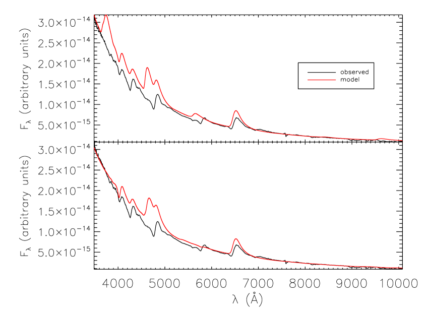
Figure 1: . The observed spectrum on Jul 02, 2005 is compared to a model spectrum using solar abundances (top panel) and CNO enhanced abundances (bottom panel). The observed spectrum has been dereddened using $E(B-V)=0.11$. In this and subsequent plots the model and observations have been normalized at 8000 $\mathrm{\AA}$.

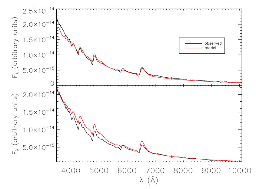
Figure 2: . The observed spectrum on Jul 02, 2005 is compared to a model spectrum using solar abundances (top panel) and CNO enhanced abundances (bottom panel). The observed spectrum has been dereddened using $E(B-V)=0.035$.

4 Abundances

Typically, the approach to obtaining abundances in differentially expanding flows has been through line identifications. This method has been successful using the SYNOW code (see Branch et al., 2005, 2006, and references therein) as well as the work of Mazzali and collaborators (for example Stehle et al., 2005). Nevertheless, line identifications do not provide direct information on abundances, which are what are input into stellar evolution calculations and output from hydrodynamical calculations of supernova explosions and nucleosynthesis. Line identifications are subject to error in that there may be another candidate line that is not considered in the analysis or there may be two equally valid possible identifications, the classic being He I $\lambda 5876$ and Na I D, which have very similar rest wavelengths and are both expected in supernovae (and have both been identified in supernovae).

Here we focus on nitrogen and sodium. Massive stars which are the progenitors of SNe II are expected to undergo CNO processing at the base of the hydrogen envelope followed by mixing due to dredge up and meridional circulation. This would lead to enhanced nitrogen and sodium and depleted carbon and oxygen. For our CNO processed models we take the abundances used by Dessart & Hillier (2005). However, significant mixing of the hydrogen and helium envelope is expected to occur during the explosion due to Rayleigh-Taylor instabilities and mass loss will occur during the pre-supernova evolution. Studies of the evolution of massive stars show that for an 11 ${\mathrm{M}_{\odot}}$ model the mass fractions of CNO are very close to solar, with significantly less depletion of carbon and oxygen than is obtained from CNO processing (A. Chieffi & M. Tavani, 2006, in preparation). A detailed study of SN 2005cs spectra using the results of these hydro models will be a sensitive test of the predictions of stellar evolution theory.

4.1 Line IDs

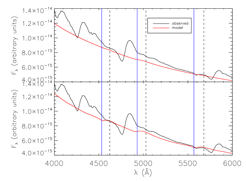
Figure 5: The observed spectrum on Jul 02, 2005 is compared to a model spectrum where only N II line opacity has been included. The top panel is for solar abundances and the bottom panel using CNO enhanced abundances. The vertical dashed lines show the rest wavelength of the N II optical lines, while the solid vertical lines show those same lines blueshifted by $v_{0}=6000$ $\mathrm{km}~{}\mathrm{s}^{-1}$. The observed spectrum has been dereddened using $E(B-V)=0.035$.

In detailed line-blanketed models such as the ones presented here line identifications are difficult since nearly every feature in the model spectrum is a blend of many individual weak and strong lines. Nevertheless, it is useful to attempt to understand just what species are contributing to the variations in the spectra. In order to do this we produce “single element spectra” where we calculate the synthetic spectrum (holding the temperature and density structure fixed) but turning off all line opacity except for that of a given species. Figure 5 shows the single element spectrum for N II for our $T_{\mathrm{model}}$ = 12000 K models with solar abundances (top panel) and CNO enhanced abundances (bottom panel). Clearly the N II lines are present in CNO enhanced models and absent in the solar models, but their effect on the total spectrum is unclear.

N II lines were first identified in SN II in SN 1990E (Schmidt et al., 1993). Using SYNOW, Baron et al. (2000) found evidence for N II in SN 1999em, however more detailed modeling with PHOENIX indicated that the lines were in fact due to high velocity Balmer and He I lines. Prominent N II lines in the optical are N II $\lambda 4623$, $\lambda 5029$, and $\lambda 5679$. Dessart & Hillier (2005) found strong evidence for N II in SN 1999em. Using SYNOW Elmhamdi et al. (in preparation) found evidence for N II in SN 2005cs, as did Pastorello et al. (2006) using the code developed by Mazzali and collaborators. Figure 2 compares solar abundances to a model with enhanced CNO abundances (Dessart & Hillier, 2005; Prantzos et al., 1986). Figure 2 shows that the CNO enhanced abundances model does somewhat better fitting the emission peak of H$\beta$ (see below), however the feature to the blue of H$\beta$, clearly well-fit in the solar abundance model is completely absent in the model with enhanced CNO abundances. Figure 3 shows the region where the optical N II lines are prominent and in particular, the N II $\lambda 5679$ is not quite in the same place as the observed feature and the two bluer lines have almost no effect.

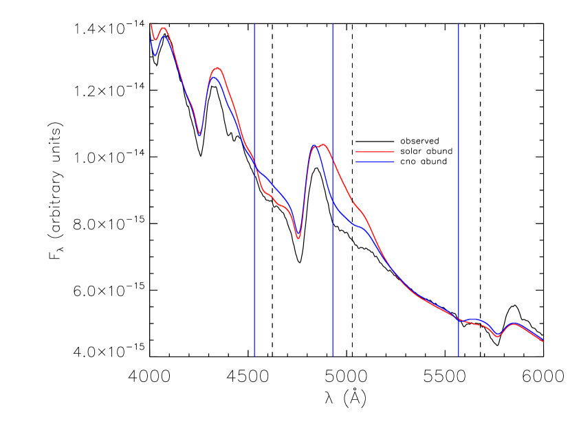
Figure 3: The observed spectrum on Jul 02, 2005 is compared to a model spectrum using CNO enhanced abundances and one using solar abundances. The region of N II lines is shown for clarity. The vertical dashed lines show the rest wavelength of the N II optical lines, while the solid vertical lines show those same lines blueshifted by $v_{0}=6000$ $\mathrm{km}~{}\mathrm{s}^{-1}$. The observed spectrum has been dereddened using $E(B-V)=0.035$.

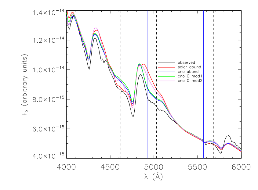
Figure 4: The observed spectrum on Jul 02, 2005 is compared to a model spectrum using CNO enhanced abundances and two where the oxygen abundance is enhanced (over the CNO value by a factor of 10 and nearly 100) in an attempt to improve the H$\beta$ emission feature and still retain the desired O II feature just blueward of H$\beta$. The plot shows how complex line IDs are. The alteration of the oxygen abundance not only affects the features, but the structure of the entire atmosphere itself (since oxygen is such a good electron donor). Neither modification is satisfactory and clearly more work needs to be done to obtain the “right” CNO abundances. The vertical dashed lines show the rest wavelength of the N II optical lines, while the solid vertical lines show those same lines blueshifted by $v_{0}=6000$ $\mathrm{km}~{}\mathrm{s}^{-1}$. The observed spectrum has been dereddened using $E(B-V)=0.035$.

We attempted to further improve the fit to the H$\beta$ emission feature by using the same abundances for C, N, and Na as our standard CNO processed abundances, but enhancing oxygen by a factor of 10 and nearly 100 (i.e. using the solar value in the latter case). Figure 4 shows how complex line IDs are. The alteration of the oxygen abundance not only affects the features, but the structure of the entire atmosphere itself (since oxygen is such a good electron donor). Neither modification is satisfactory and clearly more work needs to be done to obtain the “right” CNO abundances. Interestingly, the model with enhanced nitrogen and solar oxygen clearly shows the N II $\lambda 4623$ line.

In an attempt to identify the better fit of the feature just to the blue of H$\beta$ we examined the single element spectrum of C II (Fig. 6) since we considered that the C II $\lambda 4619$ line might be playing a role. Again this feature is clearly present in the solar model and absent in the CNO enhanced model.

Finally, we examined the lines produced by O II. Figure 7 clearly shows that O II lines play an important role in producing the observed feature just blueward of H$\beta$. Most likely it is the lines O II $\lambda 4651.5$ and $\lambda 4698$ which are producing the observed feature. On the other hand it is also clear that O II $\lambda 4915$ and $\lambda 4943$ are producing the deleterious feature just to the red of H$\beta$. Since we want somewhat higher oxygen abundances, it was natural to examine a model using the recently revised solar abundances of Asplund et al. (2005). Compared with our standard solar model abundances there was not a significant improvement (nor a degradation) in the fit to favor one over the other.

Figure 8 examines the possibility that both C II and O II contribute to the feature just blueward of H$\beta$. It is obvious that only O II lines are important for the structure of this feature.

Thus, it is clear that the strong depletion of oxygen expected from CNO processing is not evident, we can not rule out that there is some enhanced nitrogen in the observed spectra, but the N II lines don’t seem to form in the right place. However since we are studying simple, parameterized, homogeneous models this could be an artifact of our parameterization. Nevertheless, the absorption trough of the feature that we would like to attribute to N II $\lambda 5679$ is too fast in our models, whereas one would expect the CNO processed material with higher nitrogen abundance at the outermost part of the envelope and thus to form at even higher velocity due to homologous expansion. Clumping could of course change this simple one-dimensional picture.

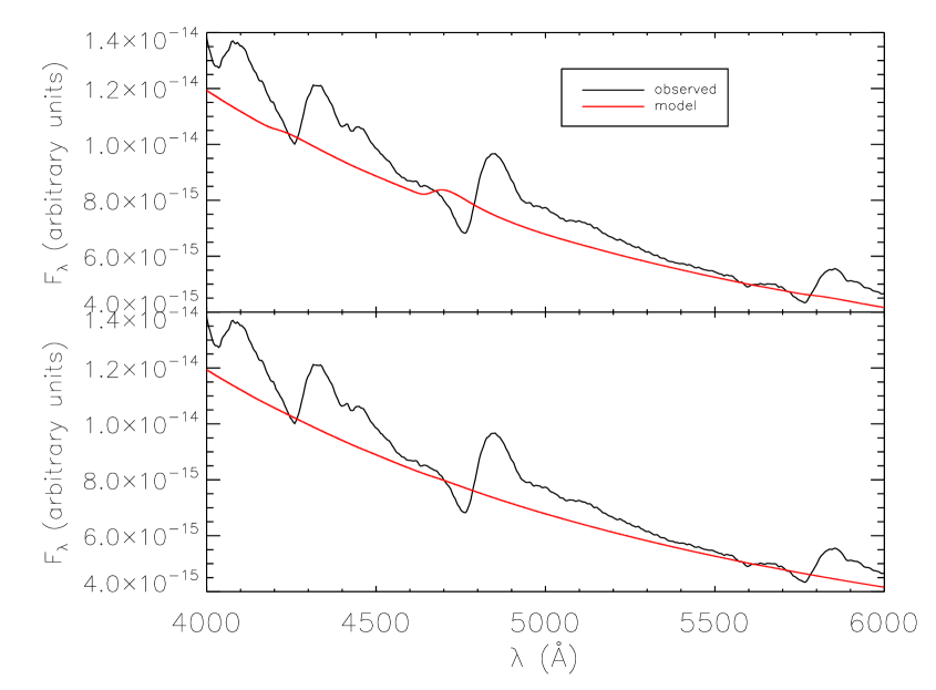
Figure 6: The observed spectrum on Jul 02, 2005 is compared to a model spectrum where only C II line opacity has been included. The top panel is for solar abundances and the bottom panel using CNO enhanced abundances. The observed spectrum has been dereddened using $E(B-V)=0.035$.

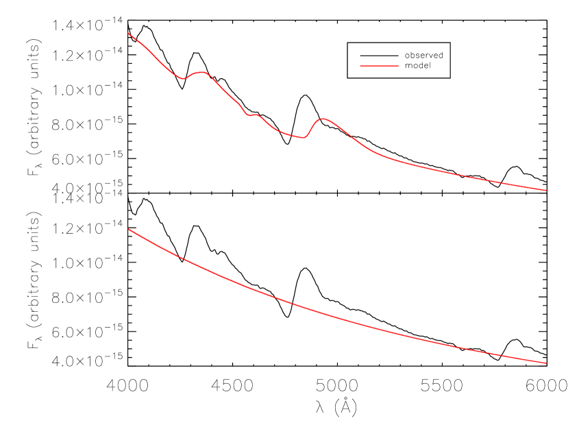
Figure 7: The observed spectrum on Jul 02, 2005 is compared to a model spectrum where only O II line opacity has been included. The top panel is for solar abundances and the bottom panel using CNO enhanced abundances. The observed spectrum has been dereddened using $E(B-V)=0.035$.

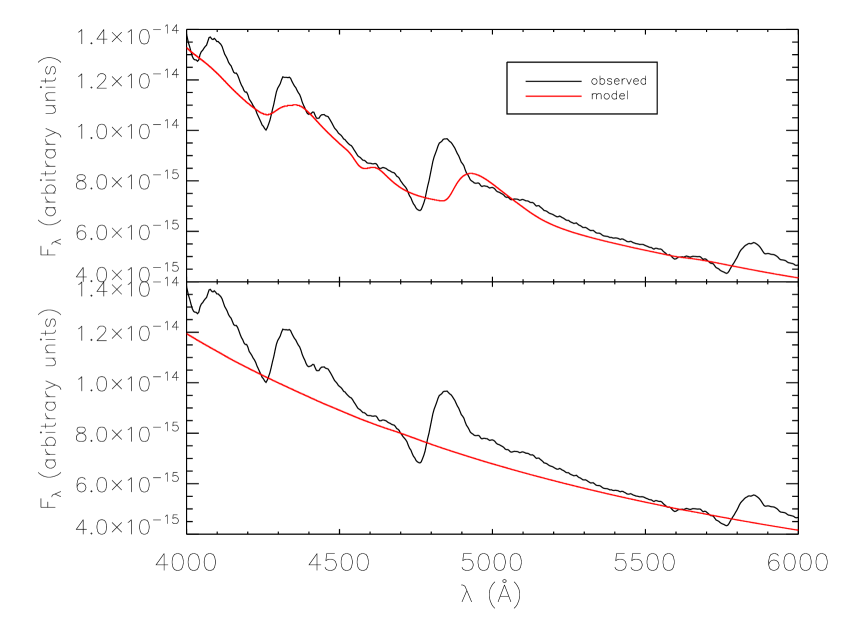
Figure 8: The observed spectrum on Jul 02, 2005 is compared to a model spectrum where only C II and O II line opacity has been included. The top panel is for solar abundances and the bottom panel using CNO enhanced abundances. The observed spectrum has been dereddened using $E(B-V)=0.035$.

5 Day 17

To examine the evolution of SN 2005cs we studied the spectrum obtained on July 14, 2005. Using our results obtained above we will take the fiducial reddening to be $E(B-V)=0.035$. Figure 9 (top panel) shows our best fit model with solar abundances. The parameters for this model were: $T_{\mathrm{model}}$ = 6000 K, $v_{0}$= 4000 $\mathrm{km}~{}\mathrm{s}^{-1}$, and $n=8$. The overall fit is quite good. The only noticeable mismatch is the trough just blueward of 5700 $\mathrm{\AA}$ is not well fit. The red part of this trough is almost certainly due to Na I D. Pastorello et al. (2006) identify the feature just to the blue as due to Ba II $\lambda$5854, which won’t be present in our models without enhanced s-process abundances or considering NLTE effects of Ba II, which is beyond the scope of this work (see below). The bottom panel of Figure 9 shows the fit with the same model parameters but CNO enhanced abundances. There is no noticeable degradation in the fit, and the enhanced sodium from CNO processing leads to a feature in the right place to fit the red part of the feature near 6000 $\mathrm{\AA}$. To further test the sensitivity to the sodium abundance, we calculated a model with solar abundances, but with sodium enhanced by a factor of ten by number. Keeping the other parameters fixed, this model is shown in Figure 10. Clearly the enhanced sodium leads to a feature at the right place that is in fact too strong. Thus, there is evidence for enhanced sodium which would most likely come from CNO processing. Overall the sodium enhanced model is a bit too cool, but we have held the other parameters fixed in order to illustrate just the effect of enhancing the sodium abundance.

Figure 9: . The observed spectrum on Jul 14, 2005 is compared to a model spectrum using solar abundances (top panel) and CNO enhanced abundances (bottom panel). The observed spectrum has been dereddened using $E(B-V)=0.035$.

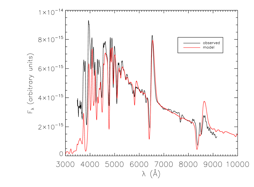
Figure 10: . The observed spectrum on Jul 14, 2005 is compared to a model spectrum using solar abundances but sodium has been enhanced by a factor of 10. The observed spectrum has been dereddened using $E(B-V)=0.035$.

6 Day 34

As our final epoch, we model spectra obtained on July 31, 2005. The parameters for this model were: $T_{\mathrm{model}}$ = 5500 K, $v_{0}$ = 6000 $\mathrm{km}~{}\mathrm{s}^{-1}$, and $n=12$. This parameter set is somewhat odd, considering that it implies that the photosphere has actually moved outward from 4000 $\mathrm{km}~{}\mathrm{s}^{-1}$ on day 17 to 6000 $\mathrm{km}~{}\mathrm{s}^{-1}$ on day 31 and that the density profile is different. This contradiction indicates the limits of our modeling with a simple single power-law and uniform compositions. Figure 11 (top panel) shows the fit with solar abundances. Overall the color is well reproduced, H$\alpha$, and both the Ca II H+K and IR triplet features are well fit, but many other lines are not, including other lines in the Balmer series. In fact while the H$\alpha$ absorption trough is quite well fit, the emission peak is too wide and too red. This is almost certainly due to our simple single power-law density profile as we will discuss in future work. Figure 11 (bottom panel) shows the fit with CNO processed abundances. As was the case for day 17, the only real improvement is that now Na I D appears in the synthetic spectrum, although it is too weak. Figure 12 shows the result of enhancing Na by a factor of ten in the solar abundance mixture, now Na I D shows up nicely, although not quite at the right velocity or strength.

Figure 13 shows a model with solar abundances, $T_{\mathrm{model}}$ = 5500 K, $v_{0}$ = 3000 $\mathrm{km}~{}\mathrm{s}^{-1}$, and $n=12$. While narrow lines appear, neither the Balmer lines nor the calcium lines are well fit and none of the absorption troughs appear at the right velocity.

Pastorello et al. (2006) found evidence for s-process elements such as barium, and charged particle elements such as scandium, which if present in our models would certainly improve the fit in Fig. 11. In our models these species are treated in LTE, but it is possible that enhanced abundances would be required to produce the strong lines observed. In studying the SN 1987A analog SN 1998A Pastorello et al. (2005) concluded that the barium lines are quite temperature sensitive and thus the difference in strength between these lines and the very strong lines observed in 1998A could well be due to NLTE effects. Utrobin & Chugai (2005) also found that the barium lines in SN 1987A was strongly dependent on the radiation field and that a full NLTE solution with a reduced UV flux due to line-blanketing reduces the need for enhanced barium abundance. Thus, with a better model for this epoch and treating barium and scandium in NLTE we are likely to get significantly improved fits, without required enhanced s-process abundances. This is a subject for future work.

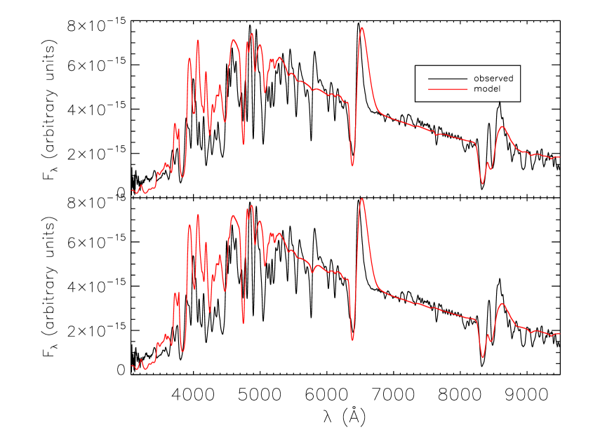
Figure 11: . The observed spectrum on Jul 31, 2005 is compared to a model spectrum using solar abundances (top panel) and CNO enhanced abundances (bottom panel). The observed spectrum has been dereddened using $E(B-V)=0.035$.

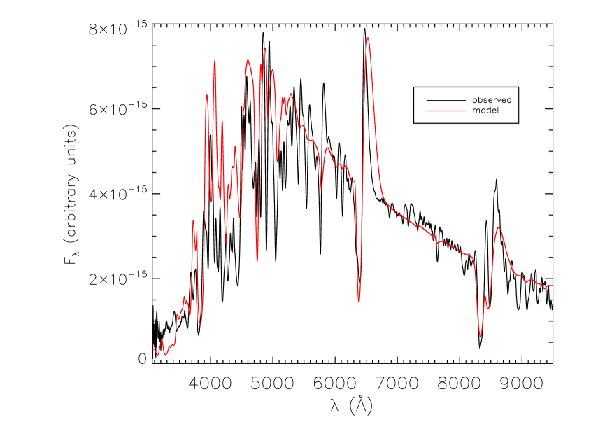
Figure 12: . The observed spectrum on Jul 31, 2005 is compared to a model spectrum using solar abundances but sodium has been enhanced by a factor of 10. The observed spectrum has been dereddened using $E(B-V)=0.035$.

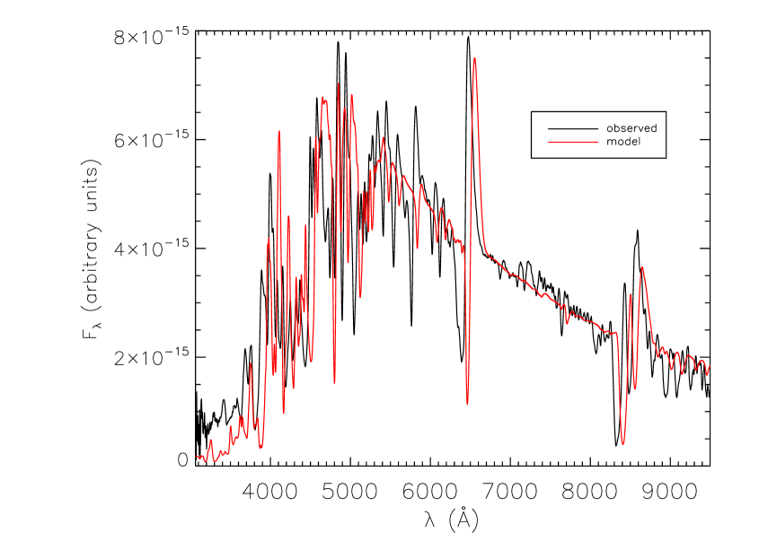
Figure 13: . The observed spectrum on Jul 31, 2005 is compared to a model spectrum using solar abundances and $v_{0}=3000$ $\mathrm{km}~{}\mathrm{s}^{-1}$. The observed spectrum has been dereddened using $E(B-V)=0.035$.

7 Distance

One method of determining distances using Type II supernovae is the “expanding photosphere method” (EPM, Kirshner & Kwan, 1974; Branch et al., 1981; Eastman & Kirshner, 1989; Schmidt et al., 1994; Eastman et al., 1996; Hamuy et al., 2001; Leonard et al., 2002) a variation of the Baade-Wesselink method (Baade, 1926). The EPM method assumes that for SNe IIP, with intact hydrogen envelopes, the spectrum is not far from that of a blackbody and hence the luminosity is approximately given by

$$L=4\pi\,\zeta^{2}\,R^{2}\,\sigma\,T^{4}$$

where $R$ is the radius of the photosphere, $T$ is the effective temperature, $\sigma$ is the radiation constant, and $\zeta$ is the “dilution factor” which takes into account that in a scattering dominated atmosphere the blackbody is diluted (Hershkowitz, Linder, & Wagoner, 1986a, b; Hershkowitz & Wagoner, 1987). The temperature is found from observed colors, so in fact is a color temperature and not an effective temperature, the photospheric velocity can be estimated from observed spectra using the velocities of the weakest lines,

$$R=v\,t,$$

the dilution factor is estimated from synthetic spectral models, and $t$ comes from the light curve and demanding self-consistency.

Both an advantage and disadvantage of EPM is that it primarily requires photometry. Spectra are only used to determine the photospheric velocity, colors yield the color temperature, which in turn is used to determine the appropriate dilution factor (from model results). This method suffers from uncertainties in determining the dilution factors, the difficulty of knowing which lines to use as velocity indicators, uncertainties between color temperatures and effective temperatures, and questions of how to match the photospheric radius used in the models to determine the dilution factor and the radius of the line forming region (Hamuy et al., 2001; Leonard et al., 2002). In spite of this the EPM method was successfully applied to SN 1987A in the LMC (Eastman & Kirshner, 1989; Branch, 1987) which led to hopes that the EPM method would lead to accurate distances, independent of other astronomical calibrators. Recently, the EPM method was applied to the very well observed SN IIP 1999em (Hamuy et al., 2001; Leonard et al., 2002; Elmhamdi et al., 2003). All three groups found a distance of 7.5–8.0 Mpc. Leonard et al. (2003) subsequently used HST to obtain a Cepheid distance to the parent galaxy of SN 1999em, NGC 1637, and found $11.7\pm 1.0$ Mpc, a value 50% larger than that obtained with EPM. Dessart & Hillier (2006) calculated updated values for the dilution factor and found good agreement with the Cepheid distance using EPM, but emphasized that dilution factors would have to be calculated for each supernova individually. Using SEAM Baron et al. (2004) found a distance to SN 1999em of $12.5\pm 2.3$ Mpc.

With modern detailed NLTE radiative transfer codes, accurate synthetic spectra of all types of supernovae can be calculated. The Spectral-fitting Expanding Atmosphere Method (SEAM, Baron et al., 1995a, 1996; Lentz et al., 2001; Mitchell et al., 2002) was developed using the generalized stellar atmosphere code PHOENIX (for a review of the code see Hauschildt & Baron, 1999). While SEAM is similar to EPM in spirit, it avoids the use of dilution factors and color temperatures. Velocities are determined accurately by actually fitting synthetic and observed spectra. The radius is still determined by the relationship $R=vt$, (which is an excellent approximation because all supernovae quickly reach homologous expansion) and the explosion time is found by demanding self consistency. SEAM uses all the spectral information available in the observed spectra simultaneously which broadens the base of parameter determination. Since the spectral energy distribution is known completely from the calculated synthetic spectra, one may calculate the absolute magnitude, $M_{X}$, in any photometric band $X$,

$$M_{X}=-2.5\log\int_{0}^{\infty}S_{X}(\lambda)\,L_{\lambda}\,d\lambda+C_{X}\,$$

where $S_{X}$ is the response of filter $X$, $L_{\lambda}$ is the luminosity per unit wavelength, and $C_{X}$ is the zero point of filter $X$ determined from standard stars. Then one immediately obtains a distance modulus $\mu_{X}$, which is a measure of the distance

$$\mu_{X}\equiv m_{X}-M_{X}-A_{X}-K_{x}=5\log{(d/10\textrm{pc})},$$

where $m_{X}$ is the apparent magnitude in band $X$, $A_{X}$ is the extinction due to dust along the line of sight both in the host galaxy and in our own galaxy, and $K_{X}$ is the k-correction (Oke & Sandage, 1968). The SEAM method does not need to invoke a blackbody assumption or to calculate dilution factors.

We calculate a SEAM distance to SN 2005cs using our first two early dates, day 5 and day 17, since our best fit to day 34 was contradictory in that the photosphere moved out and the density slope was different at a previous time. With only two days we don’t have much leverage on the time of explosion, thus we adopt the explosion time of Pastorello et al. (2006). Using 5 photometric bands $UBVRI$ and our adopted reddening of $E(B-V)=0.035$ we find $\mu=29.5\pm 0.18$ which corresponds to a distance of $7.9^{+0.7}_{-0.6}$ Mpc where the error is just the formal $1-\sigma$ error and does not include systematic error. Using the EPM method Takáts & Vinkó (2006) found $D=7.59\pm 1.02$ Mpc, and using a standard candle method (Hamuy, 2003; Nugent et al., 2006) they found $D=6.02\pm 1.3$ Mpc. Using the SEAM method on SN 1994I a Type Ic that is also in M51 we found $D=6.02\pm 1.92$ Mpc (Baron et al., 1996). Given that SNe Ic are much more difficult to model than SNe II, the fact that the two SEAM results agree within the errors is strong evidence that not only is the SEAM method robust, but the errors can be reasonably well estimated. Takáts & Vinkó (2006) summarize the other distance estimates obtained to M51 and find an average value of $D=7.1\pm 1.2$ Mpc. Given the wide range of distances obtained and the relative closeness of M51, an effort should be made to obtain a Cepheid distance to M51.

8 Discussion and Conclusions

We have calculated a small grid of simple parameterized explosion models for SN 2005cs. We have shown that the reddening estimated in previous studies is likely too high and we adopted the lowest possible value, that of foreground reddening alone. Additionally we have shown that while there is evidence for enhanced nitrogen and sodium as would be expected from CNO processing in the pre-supernova envelope, the specific set of abundances that we adopted were too depleted in oxygen to match the observed spectrum. We have not attempted to exhaust the full parameter space and determine exact abundances in this work, merely to show that such an approach is feasible given sufficient computational resources. Additionally, we had trouble obtaining a physically plausible fit to the final epoch we studied, 34 days past explosion. All of these shortcomings point that a better approach would be to run large grids using the best current stellar evolution models and compare the results to many well-observed SNe IIP. This should be feasible in the near future. Using the SEAM method we obtained a distance to M51 which is somewhat larger than the accepted distance. The SEAM method has been shown to be reliable in modeling SNe IIP and our result is reliable enough that it should be calibrated with a Cepheid distance to M51. This could then be compared with the results from a larger more homogeneous grid.

References

- Arnett et al. (1989) Arnett, W. D., Bahcall, J., Kirshner, R. P., & Woosley, S. E. 1989, Ann. Rev. Astr. Ap., 27, 629
- Asplund et al. (2005) Asplund, M., Grevesse, N., & Sauval, A. J. 2005, in ASP Conf. Ser. 336: Cosmic Abundances as Records of Stellar Evolution and Nucleosynthesis, ed. T. G. Barnes, III & F. N. Bash, 25
- Baade (1926) Baade, W. 1926, Astr. Nach., 228, 359
- Baron & Hauschildt (1998) Baron, E. & Hauschildt, P. H. 1998, ApJ, 495, 370
- Baron et al. (1995a) Baron, E., Hauschildt, P. H., Branch, D., Austin, S., Garnavich, P., Ann, H. B., Wagner, R. M., Filippenko, A. V., Matheson, T., & Liebert, J. 1995a, ApJ, 441, 170
- Baron et al. (1996) Baron, E., Hauschildt, P. H., Branch, D., Kirshner, R. P., & Filippenko, A. V. 1996, MNRAS, 279, 799
- Baron et al. (1995b) Baron, E., Hauschildt, P. H., & Young, T. R. 1995b, Physics Reports, 256, 23
- Baron et al. (2004) Baron, E., Nugent, P., Branch, D., & Hauschildt, P. 2004, ApJ, 616, 91
- Baron et al. (2003) Baron, E., Nugent, P. E., Branch, D., Hauschildt, P. H., Turatto, M., & Cappellaro, E. 2003, ApJ, 586, 1199
- Baron et al. (2000) Baron, E. et al. 2000, ApJ, 545, 444
- Blinnikov (1999) Blinnikov, S. 1999, Astronomy Letters, 25, 359
- Blinnikov et al. (2000) Blinnikov, S., Lundqvist, P., Bartunov, O., Nomoto, K., & Iwamoto, K. 2000, ApJ, 532, 1132
- Branch (1987) Branch, D. 1987, ApJ, 320, L23
- Branch et al. (2005) Branch, D., Baron, E., Hall, N., Melakayil, M., & Parrent, J. 2005, PASP, 117, 545
- Branch et al. (2006) Branch, D., Dang, L. C., Hall, N., Ketchum, W., Melakayil, M., Parrent, J., Troxel, M. A., Casebeer, D., Jeffery, D. J., & Baron, E. 2006, PASP, 118, 560
- Branch et al. (1981) Branch, D., Falk, S. W., McCall, M. L., Rybski, P., Uomoto, A. K., & Wills, B. J. 1981, ApJ, 244, 780
- Cardelli et al. (1989) Cardelli, J. A., Clayton, G. C., & Mathis, J. S. 1989, ApJ, 345, 245
- Chevalier (1984) Chevalier, R. A. 1984, Ann. NY Acad. Sci., 422, 215
- Dahlén & Fransson (1999) Dahlén, T. & Fransson, C. 1999, A&A, 350, 349
- Dessart & Hillier (2005) Dessart, L. & Hillier, D. J. 2005, A&A, 437, 667
- Dessart & Hillier (2006) —. 2006, A&A, 447, 691
- Eastman & Kirshner (1989) Eastman, R. & Kirshner, R. P. 1989, ApJ, 347, 771
- Eastman et al. (1996) Eastman, R., Schmidt, B. P., & Kirshner, R. 1996, ApJ, 466, 911
- Elmhamdi et al. (2003) Elmhamdi, A., Danziger, I. J., Chugai, N., Pastorello, A., Turatto, M., Cappellaro, E., Altavilla, G., Benetti, S., Patat, F., & Salvo, M. 2003, MNRAS, 338, 939
- Feldmeier et al. (1997) Feldmeier, J. J., Ciardullo, R., & Jacoby, G. H. 1997, ApJ, 479, 231
- Fisher et al. (1999) Fisher, A., Branch, D., Hatano, K., & Baron, E. 1999, MNRAS, 304, 67
- Grevesse & Sauval (1998) Grevesse, N. & Sauval, A. J. 1998, Space Science Reviews, 85, 161
- Hamuy (2003) Hamuy, M. 2003, in Measuring and Modeling the Universe, ed. W. L. Freedman, Carnegie Observatories Astrophysics Series, Vol. 2 (Cambridge: Cambridge Univ. Press)
- Hamuy et al. (2001) Hamuy, M. et al. 2001, ApJ, 558, 615
- Hauschildt & Baron (1999) Hauschildt, P. H. & Baron, E. 1999, J. Comp. Applied Math., 109, 41
- Hauschildt et al. (1997a) Hauschildt, P. H., Baron, E., & Allard, F. 1997a, ApJ, 483, 390
- Hauschildt et al. (1996) Hauschildt, P. H., Baron, E., Starrfield, S., & Allard, F. 1996, ApJ, 462, 386
- Hauschildt et al. (1997b) Hauschildt, P. H., Schwarz, G., Baron, E., Starrfield, S., Shore, S., & Allard, F. 1997b, ApJ, 490, 803
- Hershkowitz et al. (1986a) Hershkowitz, S., Linder, E., & Wagoner, R. 1986a, ApJ, 301, 220
- Hershkowitz et al. (1986b) —. 1986b, ApJ, 303, 800
- Hershkowitz & Wagoner (1987) Hershkowitz, S. & Wagoner, R. 1987, ApJ, 322, 967
- Khokhlov et al. (1999) Khokhlov, A. M., Höflich, P. A., Oran, E. S., Wheeler, J. C., Wang, L., & Chtchelkanova, A. Y. 1999, ApJ, 524, L107
- Kirshner & Kwan (1974) Kirshner, R. P. & Kwan, J. 1974, ApJ, 193, 27
- Kloehr et al. (2005) Kloehr, W., Muendlein, R., Li, W., Yamaoka, H., & Itagaki, K. 2005, IAU Circ., 8553, 1
- LeBlanc & Wilson (1970) LeBlanc, J. & Wilson, J. R. 1970, ApJ, 161, 541
- Lentz et al. (2001) Lentz, E., Baron, E., Branch, D., & Hauschildt, P. H. 2001, ApJ, 557, 266
- Leonard et al. (2000) Leonard, D., Filippenko, A. V., & Matheson, T. 2000, in Cosmic Explosions, ed. S. Holt & W. Zhangl, AIP Conf. Proc. 522 (New York: AIP), 165
- Leonard et al. (2006) Leonard, D. C., Filippenko, A. V., Ganeshalingam, M., Serduke, F. J. D., Li, W., Swift, B. J., Gal-Yam, A., Foley, R. J., Fox, D. B., Park, S., Hoffman, J. L., & Wong, D. S. 2006, Nature, 440, 505
- Leonard et al. (2002) Leonard, D. C. et al. 2002, PASP, 114, 35
- Leonard et al. (2003) —. 2003, ApJ, 594, 247
- Li et al. (2006) Li, W., Van Dyk, S. D., Filippenko, A. V., Cuillandre, J.-C., Jha, S., Bloom, J. S., Riess, A. G., & Livio, M. 2006, ApJ, 641, 1060
- Maund et al. (2005) Maund, J., Smartt, S., & Danziger, I. J. 2005, MNRAS, 364, L33
- Miralda-Escudé & Rees (1997) Miralda-Escudé, J. & Rees, M. J. 1997, ApJ, 478, L57
- Mitchell et al. (2002) Mitchell, R., Baron, E., Branch, D., Hauschildt, P. H., Nugent, P., Lundqvist, P., Blinnikov, S., & Pun, C. S. J. 2002, ApJ, 574, 293
- Mitchell et al. (2001) Mitchell, R., Baron, E., Branch, D., Lundqvist, P., Blinnikov, S., Hauschildt, P. H., & Pun, C. S. J. 2001, ApJ, 556, 979
- Nugent et al. (2006) Nugent, P., Sullivan, M., Ellis, R., Gal-Yam, A., Leonard, D. C., Howell, D. A., Astier, P., Carlberg, R. G., Conley, A., Fabbro, S., Fouchez, D., Neill, J. D., Pain, R., Perrett, K., Pritchet, C. J., & Regnault, N. 2006, ApJ, 645, 841
- Oke & Sandage (1968) Oke, J. B. & Sandage, A. 1968, ApJ, 154, 21
- Pastorello et al. (2005) Pastorello, A., Baron, E., Branch, D., Zampieri, L., Turatto, M., Ramina, M., Benetti, S., Cappellaro, E., Salvo, M., Patat, F., Piemonte, A., Sollerman, J., Leibundgut, B., & Altavilla, G. 2005, MNRAS, 360, 950
- Pastorello et al. (2006) Pastorello, A. et al. 2006, MNRAS, 370, 1752
- Prantzos et al. (1986) Prantzos, N., Doom, C., de Loore, C., & Arnould, M. 1986, ApJ, 304, 695
- Schlegel et al. (1998) Schlegel, D., Finkbeiner, D., & Davis, M. 1998, ApJ, 500, 525
- Schmidt et al. (1993) Schmidt, B. et al. 1993, AJ, 105, 2236
- Schmidt et al. (1994) Schmidt, B. P. et al. 1994, ApJ, 432, 42
- Stehle et al. (2005) Stehle, M., Mazzali, P., Benetti, S., & Hillebrandt, W. 2005, MNRAS, 360, 1231
- Takáts & Vinkó (2006) Takáts, K. & Vinkó, J. 2006, MNRAS
- Tammann et al. (2003) Tammann, G. A., Sandage, A., & Reindl, B. 2003, A&A, 404, 423
- Utrobin & Chugai (2005) Utrobin, V. P. & Chugai, N. N. 2005, A&A, 441, 271
- Wang et al. (1996) Wang, L., Wheeler, J. C., Li, Z., & Clocchiatti, A. 1996, ApJ, 467, 435
- Yungelson & Livio (2000) Yungelson, L. R. & Livio, M. 2000, ApJ, 528, 108