Forward modelling of sub-photospheric flows for time-distance helioseismology

Abstract

Aims.

Methods.

Results.

Abstract

Context. Results of forward modelling of acoustic wave propagation in a realistic solar sub-photosphere with two cases of steady horizontal flows are presented and analysed by the means of local helioseismology.

Aims. This paper is devoted to an analysis of the influence of steady flows on the propagation of sound waves through the solar interior.

Methods. The simulations are based on fully compressible ideal hydrodynamical modelling in a Cartesian grid. The initial model is characterised by solar density and pressure stratifications taken from the standard Model S and is adjusted in order to suppress convective instability. Acoustic waves are excited by a non-harmonic source located below the depth corresponding to the visible surface of the Sun. Numerical experiments with coherent horizontal flows of linear and Gaussian dependences of flow speed on depth are carried out. These flow fields may mimic horizontal motions of plasma surrounding a sunspot, differential rotation or meridional circulation. An inversion of the velocity profiles from the simulated travel time differences is carried out. The inversion is based on the ray approximation. The results of inversion are then compared with the original velocity profiles.

Results. Results of forward modelling of acoustic wave propagation in a realistic solar sub-photosphere with two cases of steady horizontal flows are presented. The influence of steady flow on the propagation of sound waves through the solar interior is analysed. A time-distance analysis technique is applied to compute the direct observable signatures of the background bulk motions on travel times and phase shifts. This approach allows direct comparison with observational data. Further, we propose a method of obtaining the travel-time differences for the waves propagating in sub-photospheric solar regions with horizontal flows. The method employs directly the difference between travel-time diagrams of waves propagating with and against the background flow.

Conclusions. The analysis shows that the flow speed profiles obtained from inversion based on the ray approximation differ from the original ones. The difference between the original and observed profiles is caused by the fact that the wave packets propagate along the ray bundle, which has a finite extent, and thus reach deeper regions of the sub-photosphere in comparison with ray theory.

1 Introduction

Recent observational studies in local time-distance helioseismology show the existence of large-scale motions of plasma in the sub-photospheric regions of the Sun (see, for example, a general review of recent findings in theoretical and observational local and time-distance helioseismology by Gizon & Birch (2005)). These flows can be caused, for example, by interaction of the magnetic field with the plasma in the sunspots, by differential rotation, or by meridional circulation. An initial, encouraging analyses of sub-photospheric flows in the limit of short wavelength (ray approximation) has been carried out by Giles (1999). Time-distance helioseismology in the ray approximation has also been used to map the flow structures beneath sunspots (Kosovichev et al., 2000; Zhao et al., 2001; Zhao & Kosovichev, 2003). The presence of long-lived large-scale subphotospheric convective flows has been studied by Haber et al. (1998, 2001) using ring-diagram analysis. Surface gravity waves have been used in the studies of Corbard & Thompson (2002) to analyze radial gradients of angular velocity in the solar subsurface regions down to 15 Mm. Progress in the analytical analysis of solar sub-photosphere with a homogeneous background flow has been shown by Erdélyi & Taroyan (2001) and Taroyan (2004).

The measurement accuracy of solar observations is continually changing with the improvement of observational technology, thus requiring more precise methods of data analysis and giving a need for artificial (synthetic) data produced by modelling simulations, which are able to mimic observations with a required precision. The approach of forward modelling of sound speed inhomogeneities in homogeneous solar interior models was used to explore the validity conditions of the Born and ray approximations by Birch & Kosovichev (2000). Also, a study of the validity of the ray and Born approximations in analyzing the sensitivity of wave travel times to background flows, based on the forward modelling of acoustic wave propagation in a constant background density and pressure, has been done by Birch & Felder (2004), Gizon & Birch (2005). Later, a limited approach using numerical solution of the wave equation with solar sound speed and density profiles has been applied to analyse seismic traces produced by propagation of acoustic waves, see e.g. Tong et al. (2003). In a recent work of Shelyag et al. (2006) the ability of full forward modelling to successfully reproduce the observed power spectrum of solar oscillations and seismic traces by excitation of sound waves by single and multiple random acoustic sources has been shown.

In this paper, an analysis is presented of the results of the forward modelling of acoustic wave propagation in the solar sub-photosphere with two types of sub-photospheric steady horizontal flows. The full set of compressible hydrodynamic equations is solved in order to provide the artificial data. The initial model is calculated from the standard Model S (Christensen-Dalsgaard et al., 1996), and is modified in order to suppress convective instability in the originally convectively unstable solar sub-photosphere. Flows with Gaussian and linear velocity dependences on depth are analysed in the terms of the techniques of local time-distance helioseismology. The travel times and travel-time differences are computed from the time-dependent simulations and are compared with results calculated using the ray approximation.

In the next section we give a brief description of the simulation setup and outline briefly the numerical methods used to produce the artificial data. In Section 3, the simulations, their direct interpretation and data measurements in terms of time-distance helioseismology are shown. Further, the method of obtaining travel-time differences from the artificial data is discussed in this section. In Section 4, we compare the travel-time differences obtained from forward modelling with those calculated using the ray approximation. The inversion technique, the flow profiles obtained by inversion of the travel-time differences, and their comparison with the original sub-photospheric flow velocity profiles are presented in Section 5. The results and conclusions are discussed in Section 6.

2 Simulation setup

The simulation model box has been described by Shelyag et al. (2006). For convenience, we briefly describe the setup here. The Versatile Advection Code (VAC), originally developed by Tóth et al. (1998), is implemented here to carry out the forward modelling. VAC solves numerically a set of hyperbolic equations by a number of different computational methods in one, two or three dimensions in Cartesian, cylindrical or spherical geometries with uniform or non-uniform grids. The code was specifically set here to solve the ideal hydrodynamic equations in a two-dimensional Cartesian domain with three-dimensional vector quantities:

$$\frac{\partial\rho}{\partial t}+\nabla\cdot\left(\bf{v}\rho\right)=0,$$ (1)

$$\frac{\partial{\left(\rho\bf{v}\right)}}{\partial t}+\nabla\cdot\left(\bf{v}\rho\bf{v}\right)+\nabla p=\rho{\bf{g}},$$ (2)

$$\frac{\partial{e}}{\partial{t}}+\nabla\cdot\left({\bf{v}}e+{\bf{v}}p\right)=\rho{\bf{g}}\cdot{\bf{v}}+Q\left({\bf{r}},t\right),$$ (3)

$$p=\left(\Gamma_{1}-1\right)\left(e-\frac{\rho{\bf{v}}^{2}}{2}\right),$$ (4)

where $\rho$ is the density, ${\bf{v}}=\left(v_{x},0,v_{z}\right)$ is the two-dimensional velocity vector, $e=\epsilon+\rho{\bf{v}}^{2}/2$ is the total energy density per unit volume, $\epsilon=p/\left(\Gamma_{1}-1\right)$, $p$ is the kinetic gas pressure, $\Gamma_{1}$ is the adiabatic index, ${{\bf{g}}=\left(0,0,g\right)}$ is the solar gravitational acceleration vector, $Q$ is the temporally and spatially dependent term describing additional energy sources, and $t$ is time.

A Total Variation Diminishing (TVD) spatial and a fourth-order Runge-Kutta time discretisation schemes are used. The simulation domain is shown in Fig. 1. The box is 150 Mm wide and 50 Mm deep, and has a resolution of 960x4000 grid points; the upper boundary of the domain is near the solar temperature minimum (see Fig. 1). The boundaries of the domain are open with zero gradients across the boundaries. Two boundary regions with $\bf{g}=0$ at the top and bottom boundaries of the box are introduced in order to simultaneously keep the domain in the pressure equilibrium and to satisfy the boundary conditions.

Figure 1: The simulation domain. The measurement level is marked by the dashed line. The temperature profile is also sketched on the plot.

The equation of state in the code is used in the form, which describes the properties of an ideal gas. The adiabatic index $\Gamma_{1}$, assumed to be constant over the computational domain, is equal to 5/3. The pressure equilibrium and modified convective stability conditions with constant solar gravity acceleration are applied to calculate the other quantities (Shelyag et al., 2006). The upper density value and convective instability dependence (Schwartzschild criterion) taken from Christensen-Dalsgaard’s standard Model S, are used as the initial conditions for the pressure equilibrium calculation. A slight increase of $\Gamma_{1}$ in comparison to the original solar model makes most of the domain except the super-adiabatic strongly convective layer near the solar surface convectively stable. Thus, the convective instability dependence is modified in this layer in order to reach convective stability. This procedure of pressure equilibrium recalculation results in values of sound speed close to those in the Sun. The dependence of the sound speed gradient on depth in the domain is shown in Fig. 2.

Figure 2: Dependence of the gradient of the sound speed on depth in the domain.

The perturbation source is located in the upper-middle (z=2000 km below the upper boundary) of the simulation box (see Fig. 1). The measurement level for latter time-distance analysis is located at 1000 km below the upper boundary.

3 Simulations

In order to excite sound waves, a single perturbation source (see Shelyag et al., 2006), corresponding to a localised cooling event causing mass inflow and sound waves excitation (Rast, 1999), has been introduced in the simulations. The source, $dQ$, is described in the energy equation of system of hydrodynamic equations as

$$dQ=\left[1+\tanh\left(\log 3\cdot\frac{t-t_{0}}{\sigma_{1}}\right)\right]\cdot\exp\frac{\left(r-r_{0}\right)^{2}}{{\sigma_{2}}^{2}}.$$ (5)

The characteristic timescale of the source is $\sigma_{1}=120\leavevmode\nobreak\ \mathrm{s}$, the spatial extent $\sigma_{2}=0.5\leavevmode\nobreak\ \mathrm{Mm}$. The source is located in the middle of the horizontal layer at 2000 km depth of the simulation domain.

The acoustic response of the model is shown in Fig. 3. The plot shows time-distance diagram of the vertical velocity component taken at the measurement level of 1000 km below the upper boundary of the simulation domain. This level approximately corresponds to the level of the visible solar photosphere. The first (faster) and the second (slower) bounces of the sound wave, propagating in the simulated solar interior, are visible in the plot. Also, the slowest wave, propagating in the waveguide created by the simulated temperature (and sound speed) minimum, is seen in the figure.

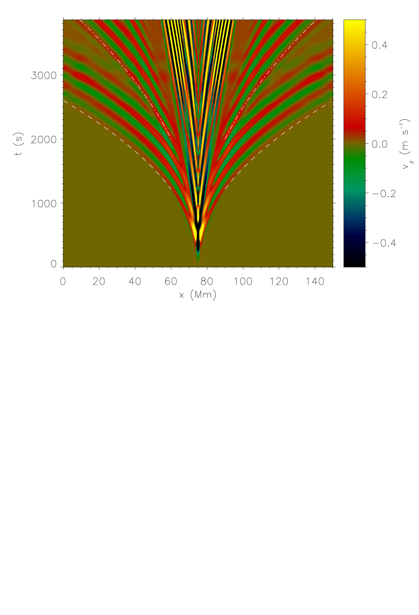
Figure 3: Time-distance diagram of the acoustic response of the model to the source. The first and second bounces are marked approximately by dashed and dash-dotted lines, respectively, and are clearly visible.

We study the influence of steady flows to the acoustic response of the simulated solar sub-photosphere. Two types of flows are introduced (see Fig. 4). The first one is a localised flow with Gaussian horizontal velocity profile. The flow centre is located at the depth of 25 Mm. The width of the flow (FWHM) is 10 Mm. The maximal flow velocity is about $300\leavevmode\nobreak\ \mathrm{m\leavevmode\nobreak\ s^{-1}}$. The flow can represent, for example, horizontal motion of solar plasma near a large sunspot. Existence of such mass flows beneath sunspots has been discovered by the means of time-distance helioseismology by Zhao et al. (2001) using the ray approximation. In this work it has been shown that localised horizontal subsonic flows with the speeds of the order of kilometre per second exist at depths of about 10 Mm and have the horizontal extent of about 30 Mm (Zhao et al., 2001, Fig. 3 in their paper), the results of inversions suggest approximate cylindrical symmetry of the flow structures under sunspots. Full magneto-hydrodynamic simulations of magneto-convection in convectively unstable cylindrically-symmetric polytropic model with presence of strong magnetic flux concentrations (Hurlburt & Rucklidge, 2000) also suggest the existence of such sub-photospheric large-scale convective flows. These flows in the simulations appear essentially weakly magnetised in comparison to strong magnetic flux concentrations, where convection is suppressed by magnetic field (Fig. 2 in Hurlburt & Rucklidge, 2000).

The second case is characterised by a linear velocity dependence on the vertical coordinate selected in the way that the velocity at the source location is equal to zero, and the velocity at the bottom of the domain is $100\leavevmode\nobreak\ \mathrm{m\leavevmode\nobreak\ s^{-1}}$. This flow can model meridional laminar circulation. Such flows have been seen observationally by Haber et al. (1998, 2001) using ring-diagram analysis of SOI-MDI observational data. Simulations of convection in spherical shells also show an evidence for meridional circulation flows with sufficiently long lifetimes (Elliott et al., 2000; Miesch et al., 2000). The average dependences of the flow speed on depth for different latitudes and Carrington longitudes, obtained by inversions of ring diagrams (Haber et al., 1998, their Figs. 5, 6), have qualitatively similar properties as the linear flow introduced to the numerical experiments presented here. The flow profiles are approximately linearly dependent on depth, and the speeds at the depth of 15 Mm are of $25-50\leavevmode\nobreak\ \mathrm{m\leavevmode\nobreak\ s^{-1}}$.

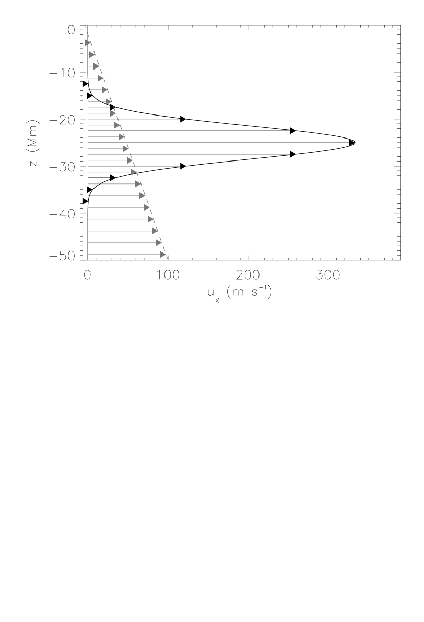
Figure 4: Sub-photospheric flow structures introduced to the simulation domain. Dashed line corresponds to the linear flow velocity profile with the maximum speed of $100\leavevmode\nobreak\ \mathrm{m\leavevmode\nobreak\ s^{-1}}$ at 50 Mm depth and zero at the source location, solid line corresponds to the Gaussian flow profile with the maximum of about $330\leavevmode\nobreak\ \mathrm{m\leavevmode\nobreak\ s^{-1}}$ and the FWHM of 10 Mm.

Since the acoustic source is equidistant from the side boundaries of the simulation box, and without a flow the wave packets would propagate symmetrically around the source, one can study effects, caused by the Doppler shift differences between the wave packets propagating to the left and to the right from the source. The numerical difference between the left and right amplitudes represents the wave phase shift.

The phase difference image for the case of the Gaussian flow profile is shown in Fig. 5, which shows the difference between the right and left portions of a time-distance diagram, such as Fig. 3. The introduced localised flow acts only on the modes which propagate deep enough in the solar sub-photosphere; the shallow modes are much less affected. This fact can be clearly seen from the figure. The phase differences are large in the regions of the first bounce propagation, however, the second and higher order bounces and the surface wave are not influenced by the flow. Also, since the flow is localised in the deep regions of sub-photosphere, where the sound speed is changing slowly, the phase difference “waves” are propagating as the waves with constant group speed corresponding to the local sound speed at the region where the influence of the flow is most significant, as can be seen from the figure.

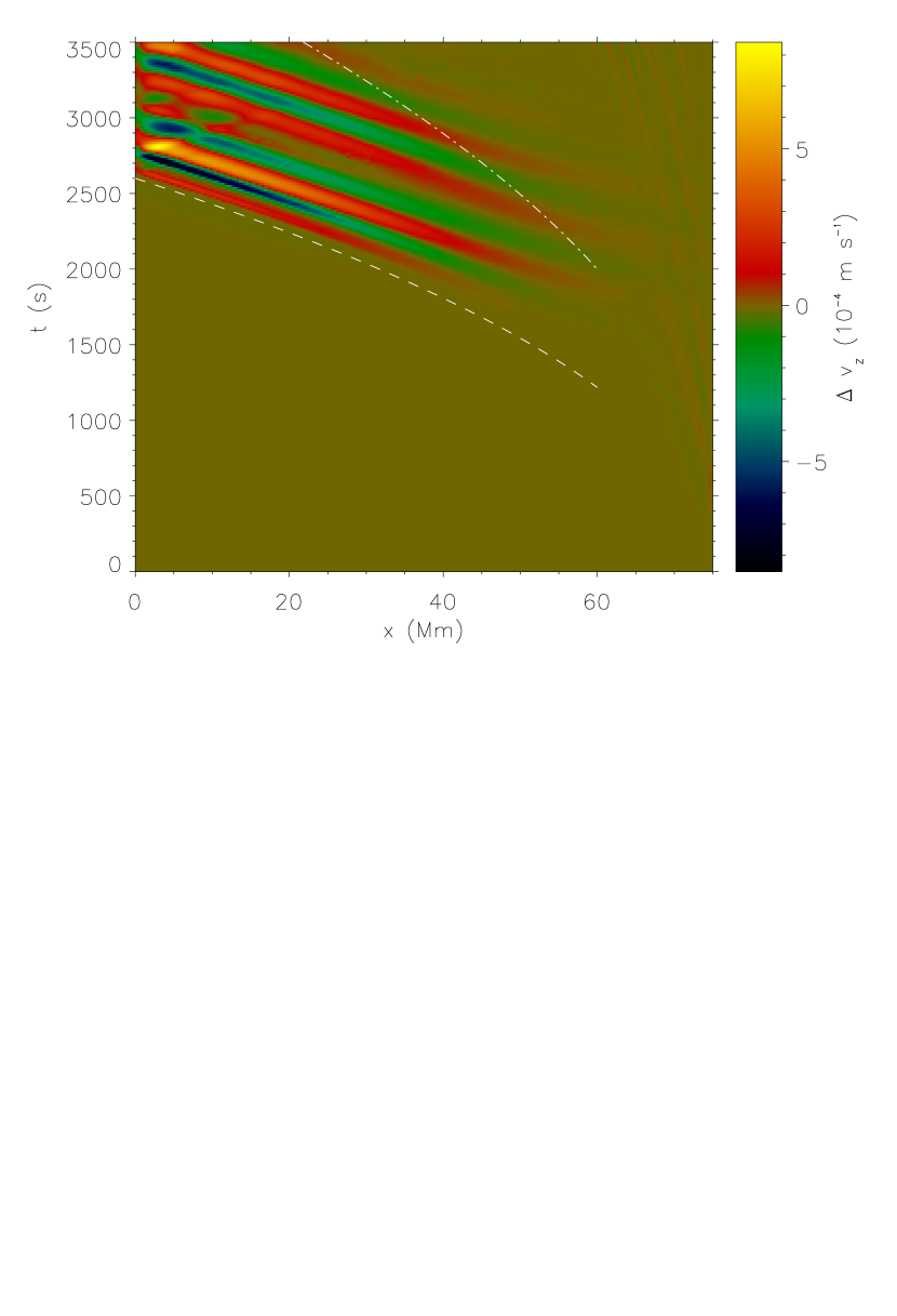
Figure 5: Vertical speed difference image for the model with the Gaussian horizontal velocity profile. The differences are computed between the points located at the same distance and opposite sides of the source. Positions of the first and second bounces in the diagram are marked by dashed and dash-dotted lines, respectively (cf. Fig. 4). The figure shows that only the first (the deepest propagating) bounce is influenced by the flow. Also, the flow acts on the wave propagating in the deeper regions with almost constant sound speed (Fig. 2), thus, the ”difference waves” travel with a constant speed, corresponding to the sound speed in the region of the model, where the influence of the flow is most significant.

The case for the linear horizontal speed profile is rather different. The phase difference plot calculated for the linear profile is shown in Fig. 6. In this case all of the modes are influenced by the flow.

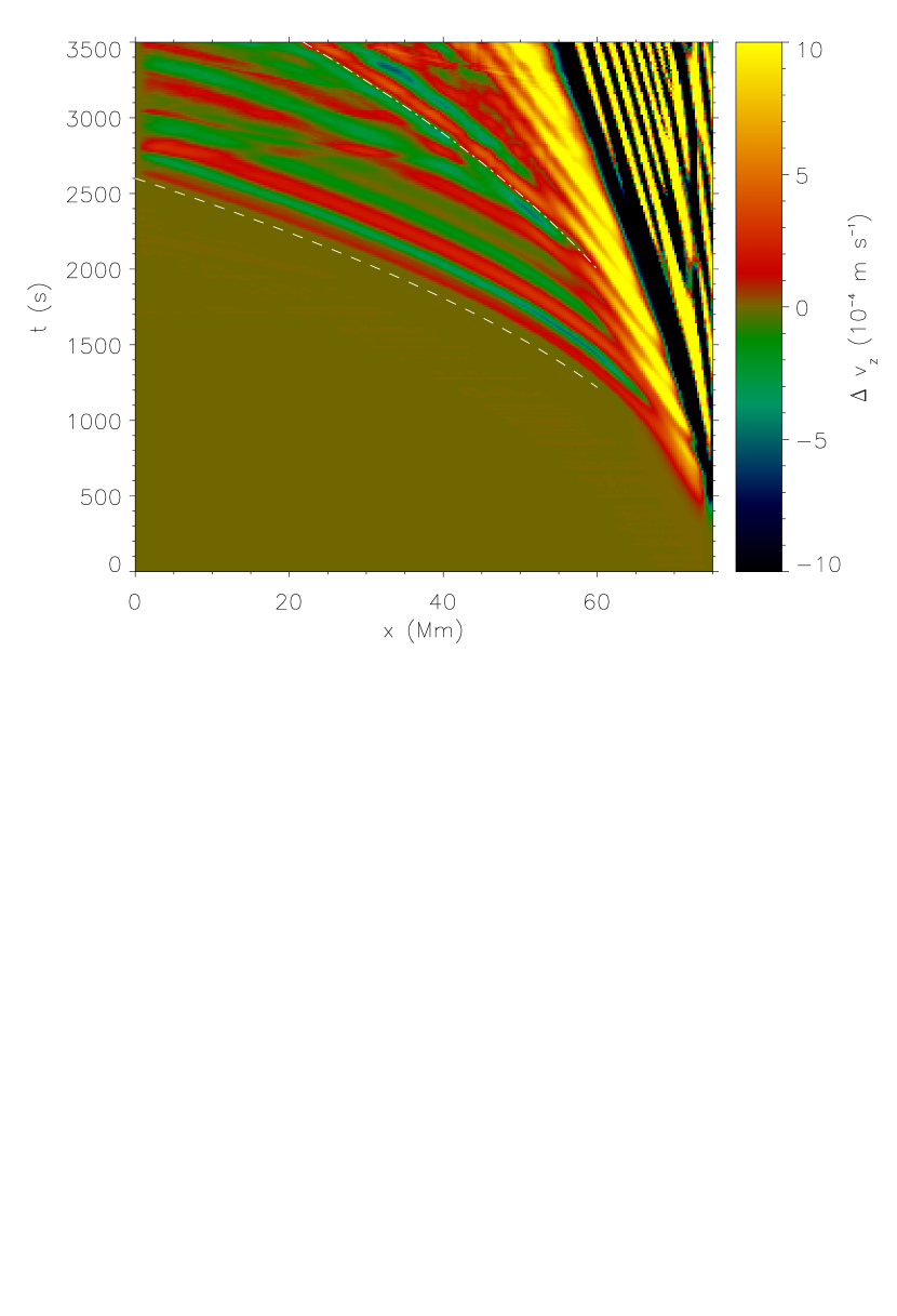
Figure 6: Vertical speed difference image for the model with the linear horizontal velocity profile Fig. 5. All modes in the box are influenced by the flow.

4 Travel-time differences

We perform the comparison of the simulated travel times with the travel times given by theoretical calculations using the ray approximation for the model depth dependences of the sound speed, pressure and density used in the numerical experiments. The simulated travel-time differences are calculated from the phase differences between the wave packets propagating to the left and to the right from the source. Assuming the harmonic response of the model to the source, the signals to the left and to the right of the source can be defined as $A_{l}=A_{0}\sin\left(\omega\left(t-\delta\tau/2\right)\right)$ and $A_{r}=A_{0}\sin\left(\omega\left(t+\delta\tau/2\right)\right)$, where $A_{0}$ is the amplitude of the wave packet, $t$ is time, and $\delta\tau/2$ is the phase shift of the wave packet with respect to the wave packet propagating in the model, undisturbed by the flow. Thus, assuming that the phase differences are less than $2\pi$ and measuring the difference $\Delta A=A_{l}-A_{r}=2A_{0}\cos\left(\omega t\right)\sin\left(\omega\cdot\delta\tau/2\right)$ from the simulations accordingly to Figs. 5 and 6 one can evaluate the time difference between the acoustic waves propagating to the left and to the right from the source:

$$\delta\tau=\frac{2}{\omega}\arcsin\frac{\Delta A/A}{2}.$$ (6)

In Eq. (6), $A_{0}$ is the amplitude of the oscillation with the frequency $\omega$, taken along the time-distance path of the wave packet, $\Delta A$ is the amplitude difference between the packets propagating to the left and to the right from the source, taken at the same place where the amplitude $A_{0}$ is taken.

In order to calculate the travel-time differences in the ray approximation, we follow the procedure described by Giles (1999), appropriately adapted the method for the Cartesian geometry used in the simulations. At the solar surface, travel-time difference between the wave packets propagating to the left and to the right from the source can be written in the form:

$$\delta\tau=\int_{z_{1}}^{z_{2}}K\cdot u\leavevmode\nobreak\ dz,$$ (7)

where $\delta\tau$ is the travel-time difference, $u$ is the horizontal flow velocity, dependent on the depth, $K$ is the integration kernel, which contains the information about the physics of the wave propagation depending on the depth. The integration limits $\left(z_{1},z_{2}\right)$ are defined by the depth range where an oscillatory mode of some frequency $\omega$ can propagate, or, in other words, by the lower ($z_{1}$) and upper ($z_{2}$) turning points for this mode.

In the ray approximation theory, the kernel $K$ is defined by the following expression:

$$K=4\frac{v_{x}}{v_{z}c^{2}}.$$ (8)

The factor 4 in Eq. (8) indicates that in the case of the simulations described above, the travel-time differences for the waves propagating to the left and to the right are the same, and that the time the acoustic mode travels from the upper turning point to the lower one is equal to the travel time in the opposite direction.

In a plain-parallel model one can write the quantities under the integral as follows:

$$v_{z}=\frac{k_{z}\omega^{3}c^{2}}{\omega^{4}-k^{2}_{x}c^{2}\omega_{BV}^{2}},$$ (9)

$$v_{x}=k_{x}\omega c^{2}\frac{\omega^{2}-\omega_{BV}^{2}}{\omega^{4}-k_{x}^{2}c^{2}\omega_{BV}^{2}},$$ (10)

where $\omega_{BV}$ is Brunt-Väisälä frequency, defined as

$$\omega_{BV}^{2}=g_{z}\left(\frac{1}{\Gamma_{1}}\frac{d\ln p}{dz}-\frac{d\ln\rho}{dz}\right),$$ (11)

$\omega_{AC}$ is the acoustic cutoff frequency, given by

$$\omega_{AC}^{2}=\frac{c^{2}}{4}\left(\frac{d\ln p}{dz}\right)^{2},$$ (12)

$k_{z}$ is vertical wavenumber,

$$k_{z}^{2}=c^{-2}\left(\omega-\omega_{AC}\right)-k_{x}^{2}\left(1-\omega_{BV}/\omega\right),$$ (13)

and, finally, $k_{x}$ is horizontal wavenumber.

The upper and lower turning points $z_{1}$ and $z_{2}$ are defined as the range where the integrand of Eq. (7) is real.

Substituting Eqs. (9)-(13) into Eq. (8), one can calculate the values of the kernel, defined by Eq. (8). However, numerical computations of the integral in Eq. (7) with this kernel around the lower turning point has to be carried out carefully due to the singularity of the integrand there. This singularity is integrable; the procedure of integration is described in details by Christensen-Dalsgaard et al. (1989).

The results of the comparison are shown in Figs. 7 and 8 for the Gaussian and linear horizontal velocity profiles, respectively. In the case of the Gaussian velocity profile (Fig. 7), the ray approximation does not give correct travel times for medium (30-60 Mm) distances. However, the difference between travel times derived between the ray approximation and the simulations diminishes on larger distances for the waves that propagate deep in the sub-photosphere.

Figure 7: Plot of travel-time difference for ”left” and ”right” propagating wave packets in the case of localized Gaussian flow profile. The solid curve corresponds to the time difference measured directly from the simulations, the dash-dotted curve is the time difference calculated using the ray approximation for density and pressure profiles used in the simulations. The ray approximation does not seem to give accurate results for small distances (and depths) in this case, however, for large distances the difference diminishes. The noise at distances about 70 Mm is caused by interference of the forward-propagating wave packet with the wave reflected from the boundary of the simulation box.

The dependence of the travel-time difference on the horizontal coordinate for the linear velocity profile shows a rather different behaviour. All of the sound waves propagating in the sub-photosphere are affected by the flow, and the difference between the ray approximation and the forward simulations grows with the distance from the centre. Also, one can notice that the trend of the dependences show qualitatively similar behaviour.

Figure 8: Same as Fig. 7, computed for the model with linear velocity depth dependence. In this case the flow is not spatially localised, and the time difference grows with the distance from the source.

The noise in the travel-time difference dependences at distances about 60-70 Mm from the source, is caused by the interference of the forward wave packet with the wave reflected from the boundary of the simulation domain, despite the reflected wave, having much lower amplitude than the one propagating toward the boundary.

Generally, it seems that the ray approximation does not give accurate enough travel times when compared with the ones derived from the simulations for the same sub-photospheric structure. This is caused by the fact that the wave packets, produced by superposition of $p$ modes, propagate along the ray bundle which follows the path given by the ray approximation, but has a finite extent (Bogdan, 1997). Thus, for the case of a Gaussian flow, the wave packets actually reach deeper layers of the sub-photosphere and become more affected by horizontal flow, then predicted by the ray approximation. This difference diminishes when the turning point of the ray path is located close to or below the maximum of the horizontal flow. The wave packets, travelling in the sub-photosphere with a linear horizontal flow with flow speeds increasing toward the bottom of the simulation box, again because of their finite extent, are more influenced by the deeper and stronger flows in comparison with those of the ray approximation. However, as it has already been noticed, the travel-time difference dependences are qualitatively similar: for example, in Fig. 8 at e.g. the distance $x$ around 10-20 Mm, both dependences show a similar feature. This is a change of inclination of the curves, which is connected to the change of sound speed gradient (cf. Fig. 2) around the depth 5-10 Mm in the sub-photosphere. This change appears at smaller distances for the simulations in comparison with the ray approximation, because the real wave packets reach the region of sub-photosphere with a smaller sound speed gradient earlier than the wave packets approximated by ray theory, due to their finite extent.

5 Inversions of velocity profiles

Next, we perform inversion of the flow velocity profiles in the domain using the ray approximation. The inversions are carried out following the procedure described by Giles (1999). In the case of spatially discretized grid, Eq. (7) can be cast in a matrix form:

$$K\cdot u=\delta\tau,$$ (14)

where $\tau=\tau_{i}$ is the vector of travel-time difference measurements, $u=u_{j}$ is the vector representing the flow speed dependence on depth, $K$ is the matrix representation of the integration kernel Eq. (8):

$$K_{ij}=4\int_{i}\frac{v_{x}}{v_{z}c^{2}}dz_{j}.$$ (15)

The integral is taken along that part of the ray path which lies within the grid element $ij$.

The inversion problem can be set as a problem of minimisation of the quantity $|Ku-\delta\tau|^{2}$ (see, for example, Press, 2002), which is equivalent to

$$K^{T}Ku=K^{T}\delta\tau.$$ (16)

In general, the problem described by Eq. (16) can be ill-posed, also the setup can deal with the noisy data, thus the operator $K^{T}K$ has to be regularised. In order to diminish the numerical noise coming from the simulations, we regularise Eq.(16) in the following way:

$$\left(K^{T}K+\gamma\Lambda\right)u=K^{T}\delta\tau,$$ (17)

where $\Lambda$ is the regularisation operator, and $\gamma$ is a parameter which controls the relative influence of regularisation on the minimisation procedure.

For the inversion problem, the system of equations Eq. (17) is solved with respect to the flow velocity profile $u$ using the singular value decomposition (Press, 2002).

The forward problem of calculating $\delta\tau$, based on the given velocity profile and model structure, has been solved using the ray approximation. Then, the obtained values of $\delta\tau$ have been used in the inversion process in order to test the method, to select the regularisation parameter $\gamma$, and to compare the flow profiles obtained from the simulations and from this calculation, consistent with the ray approximation. The regularisation parameter $\gamma$ in Eq. (17) is selected in such a way that it does not significantly change the velocity profile, obtained by inversion of the travel-time difference dependence, calculated using the ray approximation, in comparison with the original one. The linear regularisation operator of the form, describing a priori solution as a constant, is chosen for the inversion procedure.

The results of inversion are presented in Figs. 9 and 10. Solid curves in these plots correspond to the original flow profiles, the dashed ones are obtained from the inversions of the travel time differences, which have been calculated using the ray approximation for the original flow profiles, and the dash-dotted curves show the flow profiles which are obtained from the inversions of the simulated travel-time differences (Figs. 7 and 8, solid curves).

Figure 9: Inversion of the velocity profile from the travel-time difference measurements using the ray approximation. The solid line corresponds to the original flow profile. The dashed line is the velocity profile calculated from the travel-time differences obtained by integration along the ray path given by the ray approximation theory for the model thermodynamic parameters. The dash-dotted line shows the velocity profile inferred from the travel-time difference measurements of the simulations using the ray approximation. The profile, inferred from the inversion, appears to be broader and has lower maximal amplitude than the original one.

Figure 10: Same as Fig. 9, calculated for the model with linear velocity dependence on depth. The inferred profile shows larger flow velocity values than the original one at depths above approximately 25 Mm, however, it starts to decrease in the deeper sub-photospheric layers because of the geometry of the model.

In the region with approximate depth of less than 30 Mm from the solar surface, the original profile (Figs. 9 and 10, solid curves) and the profile obtained by inversion of the travel-time differences, calculated from the ray approximation (Figs. 9 and 10, dashed curves), correspond well to each other. This defines the validity range of the data inferred from the inversion procedure. In the both flow cases, the results for the regions with the depth more than about 30 Mm do not represent the flow profiles precisely, due to the geometry of the numerical setup. In the model setup the wave packets that reach the deeper regions come out of the domain through the side boundaries and do not reach the surface.

The velocity profiles, obtained by inversions of the travel-time differences, calculated from the simulations (Figs. 9 and 10, dash-dotted curves), show significantly different behaviour compared to the real flow profiles. In the simulations, the wave packet, while propagating in the sub-photosphere, is influenced by the deeper regions of it in comparison with the ray approximation. Thus, in the case of horizontal flow with the Gaussian depth dependence, the profile, obtained from the inversion, appears to be broader, and has lower maximal amplitude than the original one, because the sensitivity of the wave packet is smoothed over the range of depths. Due to a similar reason, the velocities, obtained by the inversion, in the region between 20 and 10 Mm are larger, than the velocities in the original profile.

In the case of the linear flow velocity profile, the velocity dependence, obtained by inversion, behaves in a rather different way. Above approximately 25 Mm depth level, the obtained profile shows velocities larger than the velocities of the original flow. Below 25 Mm the dependence starts to decrease toward the bottom of the model. Again, this is caused by the finite width of the wave packet. A part of the wave packet leaves the domain after it reaches the lower boundary.

Generally, the both flow profiles are consistent with the corresponding travel-time difference dependencies Figs. 7 and 8. Larger travel-time difference corresponds to larger influence of acoustic wave by the flow, which means the larger flow speed at the same depth level. For the deeper regions, the decrease of the flow speed with depth is partly due to the geometry of the simulation setup, and in the case of Gaussian flow profile the decrease is also caused by the localised nature of the introduced flow.

The width of the wave packet at a particular depth can roughly be estimated from Fig. 10. The width should not be less than the distance difference between the points on the curves of the profile obtained from inversion of the simulated data and the profile obtained using the ray approximation taken for the same value of the velocity of the flow.

6 Discussion

In this paper, analysis of the influence of sub-photospheric flows on acoustic wave propagation in the solar interior is presented. The numerical code implemented here solves the full set of compressible hydrodynamic equations in two dimensions. The initial model uses constant adiabatic index $\Gamma_{1}=5/3$ and solar Standard Model S modified in order to suppress convective instability in the solar interior, which results in values of the sound speed close to those in the Sun. Acoustic waves are generated by a source corresponding to photospheric cooling events (photospheric plumes).

Using forward modelling, the travel times and travel-time differences have been obtained and compared with the travel-time differences calculated using the ray approximation technique for two different sub-photospheric flow profiles: localised horizontal flow with Gaussian dependence of the flow speed on depth, and flow with a linear dependence of the flow speed on depth. The Gaussian flow may represent sub-photospheric plasma motion surrounding a sunspot. The linear flow may mimic large-scale flows. The comparison of the travel-time differences shows that, in the case of a Gaussian equilibrium motion centered about 20-30 Mm below the solar surface, the travel-time difference between the ray approximation and forward modelling is large at small distances from the acoustic source and diminishes at large distances. The behaviour of acoustic waves propagating in a model with linear velocity profile is different: there the travel-time difference grows with the distance from the source. This difference can be explained by including some wave effects, which are neglected in the ray approximation. Also, the discrepancy between actual travel times and those given by the ray approximation creates certain limitations which have to be taken into account in analysis of real observational data.

The influence of the wave effects has been analysed by inversion of the travel-time differences obtained for both cases of the sub-photospheric flow velocity profiles. The inversion of travel-time differences was carried out using the ray approximation. Then the dependences of the horizontal flow velocity on depth, evaluated by inversion, were compared with the original equilibrium bulk motion profiles. The comparison shows that in the depth range between 0 and 20 Mm, the velocities obtained by inversion of the modelled data appear to be larger than the original ones; however, in the case of Gaussian flow, the maximal velocity is lower for the profile obtained from inversions. This is caused by the sensitivity of the wave packet, which in reality is spread over a range of distances, while in the ray approximation the wave packet is presumed to be infinitely thin.

References

- Birch & Kosovichev (2000) Birch, A. C., Kosovichev, A. G. 2000, Sol. Phys., 192, 193
- Bogdan (1997) Bogdan, T. J. 1997, ApJ, 477, 475
- Christensen-Dalsgaard et al. (1989) Christensen-Dalsgaard, J., Gough, D. O., Thompson, M. J. 1989, MNRaS, 1989, 238, 481
- Christensen-Dalsgaard et al. (1996) Christensen-Dalsgaard, J., et al. 1996, Science, 272, 1286
- Corbard & Thompson (2002) Corbard, T., & Thompson, M. J. 2002, Sol. Phys., 205, 211
- Birch & Felder (2004) Birch, A. C., & Felder, G. 2004, ApJ, 616, 1261
- Elliott et al. (2000) Elliott, J. R., Miesch, M. S., & Toomre, J. 2000, ApJ, 533, 546
- Erdélyi & Taroyan (2001) Erdélyi, R., & Taroyan, Y. 2001, IAU Symposium, 203, 208
- Giles (1999) Giles, P. M. Time-distance measurements of large-scale flows in the solar convection zone. PhD thesis, Stanford University.
- Gizon & Birch (2005) Gizon, L., & Birch, A. C. 2005, Living Reviews in Solar Physics, 2, 6
- Haber et al. (1998) Haber, D., Hindman, B., Toomre, J., Bogart, R., Schou, J., & Hill, F. 1998, Structure and Dynamics of the Interior of the Sun and Sun-like Stars SOHO 6/GONG 98 Workshop Abstract, June 1-4, 1998, Boston, Massachusetts, p. 791, 6, 791
- Haber et al. (2001) Haber, D. A., Hindman, B. W., Toomre, J., Bogart, R. S., & Hill, F. 2001, IAU Symposium, 203, 211
- Hurlburt & Rucklidge (2000) Hurlburt, N. E., & Rucklidge, A. M. 2000, MNRAS, 314, 793
- Kosovichev et al. (2000) Kosovichev, A. G., Duvall, T. L., & Scherrer, P. H. 2000, Sol. Phys., 192, 159
- Miesch et al. (2000) Miesch, M. S., Elliott, J. R., Toomre, J., Clune, T. L., Glatzmaier, G. A., & Gilman, P. A. 2000, ApJ, 532, 593
- Press (2002) Press, W. H. 2002, Numerical recipes in C++ : the art of scientific computing by William H. Press. xxviii, 1,002 p. : ill. ; 26 cm. Includes bibliographical references and index. ISBN : 0521750334
- Rast (1999) Rast, M. P. 1999, ApJ, 524, 462
- Shelyag et al. (2006) Shelyag S., Erdélyi, R., Thompson, M. J. 2006, ApJ, 651, 576
- Taroyan (2004) Taroyan Y., MHD waves and resonant interactions in steady states, PhD Thesis, The University of Sheffield, UK, 2004.
- Tong et al. (2003) Tong, C. H., Thompson, M. J., Warner, M. R., Rajaguru, S. P., & Pain, C. C. 2003, ApJ, 582, L121
- Tóth et al. (1998) Tóth, G., Keppens, R., & Botchev, M. A. 1998, A&A, 332, 1159
- Zhao et al. (2001) Zhao, J., Kosovichev, A. G., & Duvall, T. L. 2001, ApJ, 557, 384
- Zhao & Kosovichev (2003) Zhao, J., Kosovichev, A. G. 2003, ApJ, 591, 446