On the nonlinear saturation of the magnetorotational instability near threshold
in a thin-gap Taylor-Couette setup

Abstract

We study the saturation near threshold of the axisymmetric magnetorotational instability (MRI) of a viscous, resistive, incompressible fluid in a thin-gap Taylor-Couette configuration. A vertical magnetic field, Keplerian shear and no-slip, conducting radial boundary conditions are adopted. The weakly non-linear theory leads to a real Ginzburg-Landau equation for the disturbance amplitude, like in our previous idealized analysis. For small magnetic Prandtl number (${\cal P}_{\rm m}\ll 1$), the saturation amplitude scales as ${\cal P}_{\rm m}^{2/3}$ while the magnitude of angular momentum transport scales as ${\cal P}_{\rm m}^{4/3}$. The difference with the previous scalings ($\propto{\cal P}_{\rm m}^{1/2}$ and ${\cal P}_{\rm m}$ respectively) is attributed to the emergence of radial boundary layers. Away from those, steady-state non-linear saturation is achieved through a modest reduction in the destabilizing shear. These results will be useful to understand MRI laboratory experiments and associated numerical simulations.

I Introduction

The magneto-rotational instability (MRI) is a linear instability known to occur in rotating hydromagnetic shear flows when the angular velocity decreases with distance from the rotation axis, i.e. $\partial_{R}(\Omega^{2})<0$. Although it had been known for almost half a century veli ; chandra1 ; chandra2 , the MRI acquired a renewed interest only after the influential work of Balbus & Hawley BH91 , who have shown, by means of linear stability analysis and numerical simulations, its viability in conditions locally approximating astrophysical accretion disks. Subsequent investigations of this kind (see the reviews by Balbus & Hawley BHrev ; B03 and references therein) have quite convincingly demonstrated that this instability can drive magnetohydrodynamical (MHD) turbulence in a variety of conditions, appropriate to accretion disks and more general settings as well. Within the framework of a magnetic Taylor-Couette configuration, which is relevant for the present work, the parameter dependencies (magnetic Reynolds and Prandtl numbers) of the marginal (linear) instability threshold has been previously considered RS02 ; WB02 . It was found, among other things, that the critical magnetic Reynolds number does not scale with the magnetic Prandtl number, for small values of the latter. This result carries over into the weakly nonlinear theory presented here.

Accretion disks are important and ubiquitous astrophysical objects and are thought to power as diverse systems as young stellar objects, close binary systems and active galactic nuclei. Accretion disks are flattened, high specific angular momentum (with essentially a Keplerian distribution) masses of gas, through which matter accretes onto a central object. An efficient dissipation and transport of angular momentum mechanism is needed in order to allow accretion and reconcile theoretical models with observations. Since the typical hydrodynamical Reynolds numbers (${\cal R}$) in these astrophysical flows are enormous, it has been recognized at the outset, when accretion disks were theoretically proposed SS ; LBP , that some anomalous, enhanced (conceivably turbulent) dissipation and transport must be invoked. Keplerian rotating flows are (according to the Rayleigh and other criteria) linearly stable and thus astrophysical disk turbulence can not originate from a linear instability of the kind known (and well studied) in Taylor-Couette hydrodynamical flows.

The physics of the non-linear development of the MRI, its saturation and the nature of the resulting angular momentum transport are quite complicated. Almost all of our present knowledge on this subject comes from numerical simulations, carried out by several groups (see, e.g., BH91 ; balbusfight ; BHrev ; B03 and references therein). These finite-difference simulations, even though intended for the study of the MRI in its astrophysical setting, were actually local, i.e. done for a small portion of an accretion disk, in what is known as the shearing box or sheet (hereafter, SB) formulation glb , BH91 (see the Appendix of ur04 for a formal account on this approximation). Although a lot has been learned from these simulations, the intricate processes at work are not yet fully understood and some basic physical questions remain open (see, e.g., brand ). As a result, there has recently been a growing interest to observe the instability in the laboratory, where various physical aspects can be unraveled in a controlled way. A number of groups have indeed embarked on such experimental projects, in several setups, often accompanying them by appropriate numerical calculations (e.g., jgk ; colgate ; sisan ; hollerbach ; liu_et_al ; helical , and references therein).

In comparison to the large extent of numerical and experimental work on the MRI’s nonlinear development, there have only been very few reports on analytical and semi-analytical studies on this subject. This fact seems surprising, because a very large body of work, utilizing various asymptotic approaches, has been done for other important fluid instabilities (for reviews see, e.g., manneville1 ; cross ; manneville2 ; regev ; pismen ). We are aware of only two asymptotic studies of this kind in the MRI context:

• In the first one knobloch , Knobloch & Julien investigated the saturation of the MRI in the strongly nonlinear (far from instability threshold) regime. They utilized the so-called channel modes (radially independent axisymmetric linear modes, which also happen to be exact solutions of the nonlinear problem in the SB formulation BHrev ,GX ). They performed an asymptotic calculation, in which the evolution of channel modes is followed into the nonlinear regime by gently tuning the system out of the developed short-wavelength channel mode configuration (and under a specific regime of system’s parameters). This work shows that nonlinearities saturate the system in such a way that the momentum transport scales as $({\cal RR}_{m})^{-1}$, where ${\cal R}$ and ${\cal R}_{m}$ are the hydrodynamic and magnetic Reynolds numbers, respectively (see their Eq. 4.22). The results further indicate that, by modifying the underlying shear (the “source” of instability), the system saturates while approaching solid body rotation.

• In the second study omr , hereafter UMR06, we have employed a more traditional approach - weakly nonlinear asymptotics close to the instability threshold. The problem we considered differed from previous studies in that we considered the dynamics to be restricted to a narrow (in its radial extent) channel. Our original intent was to understand the MRI under a more controlled setting - one in which the channel modes are filtered out by the imposition of no normal-flow conditions at the inner and outer boundaries of the channel. Under these conditions, arguably more appropriate to capture the physics of experimental setups, the MRI unstable mode transits into instability in a way analogous to that of Rayleigh-Bénard convection. An idealization, involving a hybrid free-slip/no-slip and conducting/insulating boundary conditions, atop the no-normal flow conditions mentioned above, allows for transparent analytical evaluations of the derived necessary quantities (similar idealizations have sometimes been used in other studies liu_et_al ) of the problem. The similarity of this formulation to other extensively studied hydrodynamical instability problems led us to the application of weakly nonlinear asymptotic techniques to examine the system’s transition into the nonlinear realm, as well as to comparison of the results to specially-designed numerical simulations. We found that, as the system is gently tuned into instability (through a suitably defined non-dimensional parameter $\epsilon$), a saturated pattern-state emerges with an amplitude of the most unstable mode evolving according to the real Ginzburg-Landau equation (GLE),

  $$\partial_{{}_{T}}A=\lambda A+D\partial^{2}_{{}_{Z}}A-\alpha|A|^{2}A=0,$$ (1)

  where $T$ and $Z$ are suitably “stretched” time and vertical coordinates and the coefficients of the equation are all real and computable from the parameters of the physical problem. In particular, the coefficient $\alpha$ was found to scale as ${\cal P}_{m}^{-1}$, where ${\cal P}_{m}$ is the magnetic Prandtl number, defined by the ratio ${\cal R}_{m}/{\cal R}$. It means that the amplitude achieved by the system in the saturated state scales as $\epsilon\sqrt{{\cal P}_{m}}$ and correspondingly, the overall angular momentum transport as $\epsilon^{2}{\cal P}_{m}$. For ${\cal R}_{m}$ fixed this transport would scale like $1/{\cal R}$ and this formulation is useful when the resistivity of the medium is set by its physical state (i.e. degree of ionization) and one wishes to estimate the effect of decreasing effective viscosity (resulting, e.g. from the inaccuracy of the numerical scheme in a simulation). These analytical scalings were found in the limit ${\cal P}_{m}\ll 1$, while for larger values of ${\cal P}_{m}$ similar trends may be expected but the coefficients have to be evaluated numerically. We have conjectured that for self-consistent boundary conditions the above general qualitative behavior should hold as well, with perhaps some change in the relevant power of ${\cal P}_{m}$ in the scalings. Our asymptotic analysis was accompanied by fully numerical spectral calculations of the original SB equations with similarly idealized boundary conditions. The analytical and numerical scalings were found to agree quite well.

In this paper we present a study of the MRI as developing in a model representing the thin-gap limit of a magnetic Taylor-Couette (hereafter mTC) configuration, in which an incompressible axisymmetric rotating flow is subject to an external vertical magnetic field. This will permit a quantitative examination of the effect of the boundary conditions on the results reported in UMR06 and confirm the conjecture on the general qualitative behavior.

The fundamental equations of motion are the same as those assumed in previous studies of the MRI (e.g. BH91 ) save for the inclusion of non-ideal effects, namely resistivity and viscosity. Solutions to these equations are sought, subject to realistic boundary conditions at the system walls, namely that of no-flow and conducting conditions. For the vertical boundary conditions we assume periodicity for the sake of simplicity and transparency. After presenting, in Section II, the relevant approximations, definitions and equations, we perform, in Section III, a linear eigenmode analysis. We identify the most unstable mode as a function of the non-dimensional parameters of the system - of which there are five: the Cowling number ${\cal C}$, the magnetic Prandtl number ${\cal P}_{m}$, the magnetic Reynolds number ${\cal R}_{m}$, and shear index $q$ (see below). We demonstrate next that this system has a transition into instability which is similar in some important aspects to that in Rayleigh-Bénard convection manneville1 ; cross ; manneville2 ; regev . We also identify the presence of a neutral, spatially constant mode representing the hand of a constant azimuthal field.

In Section IV we perform a weakly nonlinear asymptotic analysis by tuning the system away from the conditions of marginality. In this case this is done by ratcheting the background magnetic field downward from the marginal state with the magnitude of the departure from that state measured by the small parameter $\epsilon^{2}$. The full calculation, detailed in Appendices B-D, reveals that the envelope (of the marginally unstable modes) evolution is governed by two uncoupled partial differential equations: one represents the leading MRI mode and evolves according to the real GLE and the other equation, representing the evolution of the uniform azimuthal field, is a standard diffusion equation. The saturated amplitude of the leading MRI mode is demonstrated, in the ${\cal P}_{m}\ll 1$ limit, to scale as $\epsilon{\cal P}_{m}^{2/3}$ and is shown to be affected by the boundary layers appearing at the system walls. The main physical factor contributing to saturation is identified as coming from the second order (in $\epsilon$) correction to the azimuthal velocity perturbation in the limit ${\cal P}_{m}\ll 1$. This, in turn, affects the shear profile so as to stabilize the new steady configuration. We also find that the average total angular momentum transport implied under these conditions scales as $\epsilon^{2}{\cal P}_{m}^{4/3}$ for ${\cal P}_{m}\ll 1$, or as $\epsilon^{2}{\cal R}^{-4/3}$ for ${\cal R}_{m}$ fixed (and of ${\cal O}\left({1}\right)$). These results are in accord with our conjecture and expectations given in UMR06.

In the last Section we discuss the implications of our work and how it should be perceived as a part of the ongoing research efforts on various aspects of the MRI. We also provide some heuristic arguments to help understand the results. Finally, we end with a short outline of possible directions for future work of this kind.

II Assumptions, definitions and equations

The hydromagnetic equations in cylindrical coordinates chandra2 are applied to the neighborhood of a representative radial point ($r_{0}$) in the system, using the above mentioned shearing box (SB) approximation. The SB is applied here to the thin-gap limit of a Taylor-Couette setup with an imposed background vertical magnetic field. We begin by considering a steady base flow with only a constant vertical magnetic field, ${\bf B}=B_{0}{\bf\hat{z}}$, and a velocity of the form ${\bf V}=U(x){\bf{\hat{y}}}$. In this base state the velocity has a linear shear profile $U(x)=-q\Omega_{0}x$, representing an azimuthal flow about a point $r_{0}$, that rotates with a rate $\Omega_{0}$, defined from the differential rotation law $\Omega(r)\propto\Omega_{0}(r/r_{0})^{-q}$. The total pressure in the base state (divided by the constant density),

$$\Pi\equiv\frac{1}{\rho_{0}}\left(P+\frac{B_{0}^{2}}{8\pi}\right),$$

is a constant and thus its gradient is zero.

This base flow is disturbed by 3-D perturbations on the magnetic field ${\bf b}=(b_{x},b_{y},b_{z})$, as well as on the velocity - ${\bf u}=(u_{x},u_{y},u_{z})$, and on the total pressure - $\varpi$. We consider only axisymmetric disturbances, i.e. perturbations with structure only in the $x$ and $z$ directions. This results, after non-dimensionalization, in the following set of non-linear equations:

$$\frac{d{\bf u}}{dt}-2{{\Omega_{0}\bf{\hat{z}}}\times{\bf u}}-{q\Omega_{0}u_{x}{\bf{\hat{y}}}}-{\cal C}{\bf b}\cdot\nabla{\bf b}-{\cal C}B_{0}\partial_{z}{\bf b} = -\nabla\varpi+\frac{1}{{\cal R}}\nabla^{2}{\bf u},$$ (2)

$$\frac{d{\bf b}}{dt}-{\bf b}\cdot\nabla{\bf u}+{q\Omega_{0}b_{x}{\bf{\hat{y}}}}-B_{0}\partial_{z}{\bf u} = \frac{1}{{\cal R}_{{m}}}\nabla^{2}{\bf b},$$ (3)

together with an incompressibility condition and the solenoidal magnetic field constraint

$$\nabla\cdot{\bf u}\equiv\partial_{x}u_{x}+\partial_{z}u_{z}=0,\qquad\nabla\cdot{\bf b}\equiv\partial_{x}b_{x}+\partial_{z}b_{z}=0.$$ (4)

The Cartesian coordinates $x,y,z$ represent here the radial (shear-wise), azimuthal (stream-wise) and vertical directions respectively and since axisymmetry is assumed $\nabla\equiv{\bf\hat{x}}\partial_{x}+{\bf\hat{z}}\partial_{z}$ and the Laplacian is $\nabla^{2}\equiv\partial_{x}^{2}+\partial_{z}^{2}$. Lengths have been non-dimensionalized by $L$ (the shearing-box size), time $t$ by the local rotation rate $\tilde{\Omega}_{0}$ (tildes denote here dimensional quantities). Because the dimensional rotation rate of the box (about the central object) is ${\bf\tilde{\Omega}_{0}}=\tilde{\Omega}_{0}{\bf\hat{z}}$, the non-dimensional quantity $\Omega_{0}$ is formally equivalent to $1$, but we keep it to flag the Coriolis terms. Velocities have been scaled by $\tilde{\Omega}_{0}L$ and the magnetic field by the value of the background vertical field $\tilde{B}_{0}$. Thus the non-dimensional constant background field $B_{0}\equiv 1$, but again, we leave it in the equation set for later convenience (see below). The hydrodynamic pressure is scaled by $\tilde{\rho}_{0}L^{2}\tilde{\Omega}_{0}^{2}$ and the magnetic one by $\tilde{B}_{0}^{2}/(8\pi)$. The non-dimensional perturbation $\varpi$ of the total pressure divided by the density (which is equal to 1 in non-dimensional units), which survives the spatial derivatives, is thus given by

$$\varpi=p+{\cal C}\mbox{$\frac{1}{2}$}|{\bf b}|^{2},$$ (5)

where $p$ is the hydrodynamic pressure perturbation.

The non-dimensional parameter

$${\cal C}\equiv\frac{\tilde{B}_{0}^{2}}{4\pi\tilde{\rho}_{0}\tilde{\Omega}_{0}^{2}L^{2}}=\frac{\tilde{V}_{A}^{2}}{\tilde{V}^{2}}$$ (6)

is the Cowling number, measuring the relative importance of the magnetic pressure to the hydrodynamical one. It is equal to the inverse square of the typical Alfvén number ($\tilde{V}_{A}$ is the typical Alfvén speed). The Cowling number appears in the non-linear equations, together with the two Reynolds numbers

$${\cal R}\equiv\frac{\tilde{\Omega}_{0}L^{2}}{\tilde{\nu}},\qquad{\cal R}_{m}\equiv\frac{\tilde{\Omega}_{0}L^{2}}{\tilde{\eta}},$$ (7)

where $\tilde{\nu}$ and $\tilde{\eta}$ are, respectively, the microscopic viscosity and magnetic resistivity of the fluid. We shall also see that the magnetic Prandtl number, given as ${\cal P}_{m}\equiv{\cal R}_{m}/{\cal R}$, plays an important role in the nonlinear evolution of this system.

We rewrite now the equations of motion in terms of more convenient dependent variables:

$$\partial_{t}\nabla^{2}\Psi+N_{{}_{\Psi}} = {{\cal R}}^{{}^{-1}}\nabla^{4}\Psi+2\Omega_{0}\partial_{z}u_{y}+{\cal C}B_{0}\partial_{z}\nabla^{2}\Phi$$ (8)

$$\partial_{t}u_{y}+N_{{}_{u}} = {{\cal R}}^{{}^{-1}}\nabla^{2}u_{y}-\Omega_{0}(2-q)\partial_{z}\Psi+{\cal C}B_{0}\partial_{z}b_{y}$$ (9)

$$\partial_{t}\Phi+N_{{}_{\Phi}} = {{\cal R}_{m}}^{{}^{-1}}\nabla^{2}\Phi+B_{0}\partial_{z}\Psi$$ (10)

$$\partial_{t}b_{y}+N_{{}_{b}} = {{\cal R}_{m}}^{{}^{-1}}\nabla^{2}b_{y}+B_{0}\partial_{z}u_{y}-\underline{q\Omega_{0}\partial_{z}\Phi},$$ (11)

Because the flow is incompressible and $y$-independent, the radial and vertical velocities are expressed in terms of the streamfunction, $\Psi$, that is, $(u{{}_{x}},u{{}_{z}})=(\partial_{z}\Psi,-\partial_{x}\Psi)$. Also, since the magnetic field is source free, we similarly express its vertical and radial components in terms of the flux function, $\Phi$, that is, $(b{{}_{x}},b{{}_{z}})=(\partial_{z}\Phi,-\partial_{x}\Phi)$. Note that (10) combines information about the radial and vertical magnetic fields in terms of the flux and streamfunctions (e.g. liu_et_al ). In this formulation the nonlinear advection and tension terms are

$$N_{{}_{\Psi}}\equiv J(\Psi,\nabla^{2}\Psi)-{\cal C}J(\Phi,\nabla^{2}\Phi),\quad N_{{}_{u}}\equiv J(\Psi,u_{y})-{\cal C}J(\Phi,b_{y}),$$

$$\quad N_{{}_{\Phi}}\equiv J(\Psi,\Phi),\quad N_{{}_{b}}\equiv J(\Psi,b_{y})-J(\Phi,u_{y}),$$ (12)

in which the Jacobian is defined as $J(f,g)\equiv\partial_{z}f\,\partial_{x}g-\partial_{x}f\,\partial_{z}g$. The underlined term in (11), representing the transport of the perturbed radial magnetic field by the background shear flow, is instrumental for the occurrence of the MRI in this system.

The boundary conditions are periodic on the vertical boundaries of the domain and we require also that the flow be no-slip at the inner and outer boundaries. This means that $\bf u=0$ at $x=\pm 1$, i.e.

$$u_{y}=0,~{}~{}\partial_{z}\Psi=0,~{}~{}\partial_{x}\Psi=0,\qquad{\rm at}\ \ x=\pm 1.$$ (13)

Regarding the boundary conditions on the magnetic field disturbances, we posit conditions (only 2 are needed) that are consistent with the inner and outer walls being conducting, $b_{x}=0$ and $\partial_{x}b_{y}=0$ at $x=\pm 1$, i.e.

$$\partial_{z}\Phi=0,~{}~{}\partial_{x}b_{y}=0,\qquad{\rm at}\ \ x=\pm 1.$$ (14)

Note that these boundary conditions are more physically consistent than the ones we have used in UMR06, however they will call for a numerical evaluation of the eigenfunctions and the coefficients for the asymptotic analysis that result from them.

Finally, we point out that there exists an energy theorem for the above dynamical equations. Defining the total energy (per unit length in the azimuthal direction) of the disturbances in the domain as $E\equiv\mbox{$\frac{1}{2}$}\int{\left({\bf u}^{2}+{\cal C}{\bf b}^{2}\right)dxdz}$, we get, after the usual integration procedures and application of boundary conditions,

$$\frac{dE}{dt}=q\Omega_{0}\int{{\mathbb{T}}dxdz}-\frac{1}{\cal R}\int{\left(|\nabla u_{x}|^{2}+|\nabla u_{y}|^{2}+|\nabla u_{z}|^{2}\right)dxdz}-\frac{{\cal C}}{{\cal R}_{m}}\int{\left(|\nabla b_{x}|^{2}+|\nabla b_{y}|^{2}+|\nabla b_{z}|^{2}\right)dxdz},$$ (15)

where

$${\mathbb{T}}={\mathbb{T}}_{\rm R}+{\mathbb{T}}_{\rm M},\qquad{\mathbb{T}}_{\rm R}\equiv u_{x}u_{y},\quad{\mathbb{T}}_{\rm M}\equiv-{\cal C}b_{x}b_{y}.$$

${\mathbb{T}}_{\rm R}$ and ${\mathbb{T}}_{\rm M}$ are the Reynolds (hydrodynamic) and Maxwell stresses, capturing the velocity and magnetic field disturbance correlations, respectively. Statement (15) is analogous to the Reynolds-Orr relation in hydrodynamics (for which ${\mathbb{T}}={\mathbb{T}}_{\rm R}$ and ${\mathbb{T}}_{\rm R}=0$). The total stress ${\mathbb{T}}$ will be used in the asymptotic theory we develop here as the dominant expression for the evaluation of transport, occurring during the weakly nonlinear evolution of the system. The full RHS of (15), including the two dissipative terms, should obviously vanish when a saturated, steady state is reached. We discuss this in more detail in Section V.

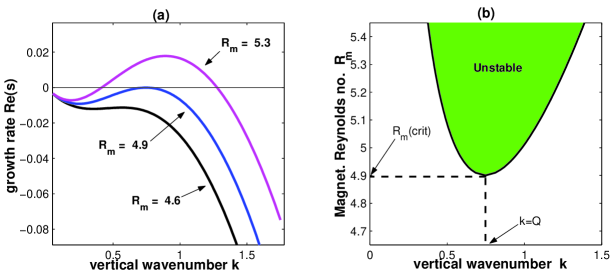
Figure 1: (Color online) Summary of linear theory. This example is for ${\cal C}=0.08$, ${\cal P}_{m}=0.001$, $q=3/2$, and the fundamental mode. (a) Growth rates, $Re(s)$, as a function of wavenumber $k$ for three values of ${\cal R}_{m}$. (b) Solid line depicts those values of ${\cal R}_{m}$ and $k$ where $Re(s)=0$. The shaded region shows unstable modes. The locations of $k=k_{crit}\equiv Q$ and ${\cal R}_{m}={\cal R}_{m}({\rm crit})\equiv R_{m}$ are shown.

III Linear Theory

Linearization of (8-11) yields the following equation

$$\partial_{t}{\cal D}{{\mathbf{V}}_{1}}={\cal L}{\mathbf{V}}_{1},$$ (16)

in which all the small perturbations are lumped in the vector ${\mathbf{V}}_{1}=\left(\Psi_{{}_{1}}(x),u_{{}_{1}}(x),\Phi_{{}_{1}}(x),b_{{}_{1}}(x)\right)^{{\mathbf{T}}}e^{ikz+st}+{\rm c.c.}$, with $k$ being the vertical wave-number and $s$ the temporal eigenvalue. The spatial differential operators $\cal D$ and $\cal L$ (appropriately written in the form of $4\times 4$ matrices) are explicitly given in (B1-B3) of Appendix B. As long as $k\neq 0$ the boundary conditions on the functions of ${\mathbf{V}}_{1}$ become (see eqs. 13-14)

$$\Psi_{{}_{1}}=D_{x}\Psi_{{}_{1}}=u_{{}_{1}}=\Phi_{{}_{1}}=D_{x}b_{{}_{1}}=0,\qquad{\rm at}\ \ x=\pm 1,$$ (17)

where $D_{x}\equiv d/dx$.

In principle, equations (16) can be set up and solved analytically however the resulting expressions are far too cumbersome to be conveniently manipulated. It is much easier to solve this set numerically, using a Chebyshev collocation technique. Each function is approximated using typically between 30 and 60 grid points on a Chebyshev numerical grid. Larger number of points are required for smaller values of the magnetic Prandtl number.

We shall concentrate on and follow here only one mode and call it the fundamental one. This is the mode which first becomes unstable when the vertical magnetic field is decreased below threshold (the mode is marginal at threshold). For given values of the parameters, the eigenvalue corresponding to this fundamental mode arises as one of the four possible solutions of the dispersion relation. It is purely real ($Im(s)=0$) and thus the instability is steady, or non-oscillatory (in the customary nomenclature, e.g., cross ). The solution of the dispersion relation provides the functional dependence $s=s(k,q,{\cal C},{\cal P}_{m},{\cal R}_{m})$.

In Figure (1-a) we display the growth rate $Re(s)$ as a function of $k$ of this fundamental mode, for several values of ${\cal R}_{m}$. The parameters ${\cal C},{\cal P}_{m}$ and $q$ are fixed at the values indicated in the caption. We see that the transition into instability is typical of steady-cellular instabilities (similar, in principle, to Rayleigh-Bénard convection). The marginal mode can be chosen to have a transition to instability at the maximum of the curve $s(k)$ (i.e. $s=0$ simultaneously with $\partial s/\partial k=0$), while all the other modes show strong temporal decay. The marginal mode can be identified with respect to a critical wavenumber $k_{\rm crit}\equiv Q$ and a critical magnetic Reynolds number ${\cal R}_{m}({\rm crit})\equiv R_{m}$.

Figure (1-b), which shows the neutral curve ($s=0$) in the ${\cal R}_{m}-k$ plane, also demonstrates the way in which the critical values $Q$ and $R_{m}$ are determined. These critical parameters are in general functions of the remaining parameters of the system, i.e. $Q=Q(q,{\cal P}_{m},{\cal C})$ and $R_{m}=R_{m}(q,{\cal P}_{m},{\cal C})$. From here on out we will restrict our considerations to values of $q=3/2$ (for consistency with UMR06) and consider the behavior of these quantities as a function of ${\cal C}$ and, primarily, ${\cal P}_{m}$.

The eigenfunctions for the mode in question have even symmetry with respect to $x=0$ due to both the symmetry in the boundary conditions and the symmetries inherent to the thin-gap limit of the mTC problem. In Figure (2) we display a sample of eigenfunctions of the marginal mode. To avoid later notational ambiguity, the eigenfunctions for these marginal modes (i.e. those with $k=Q$ and ${\cal R}_{m}=R_{m}$) will be labeled with a “11” subscript, that is, those modes will be represented by

$$\Psi_{{}_{1}}\leftrightarrow\Psi_{{}_{11}},\quad u_{{}_{1}}\leftrightarrow u_{{}_{11}},\quad\Phi_{{}_{1}}\leftrightarrow\Phi_{{}_{11}},\quad b_{{}_{1}}\leftrightarrow b_{{}_{11}},\qquad{\rm when}\ \ k=k_{\rm crit}\equiv Q,\ \ {\cal R}_{m}={\cal R}_{m}({\rm crit})\equiv R_{m}.$$

It is argued in Appendix A that in the limit ${\cal P}_{m}\ll 1$, the boundary layers size that appear scale as ${\cal P}_{m}^{1/3}$. The boundary layers that develop are satisfactorily represented numerically by the Chebyshev method used, e.g. with a grid of 50 points we can resolve at least 3-4 points of the boundary layer zones when ${\cal P}_{m}=10^{-5}$. This dependence on ${\cal P}_{m}$ will also have some bearing on the scaling properties of the coefficients of the resulting (real GLE) envelope equation, presented in the next section.

Finally, we note that there always exists an additional marginal mode of the system, separate from the above mentioned MRI mode. This neutral mode reflects a symmetry introduced into the system due to the conducting boundary conditions. Namely, a spatially constant, time-independent solution for the azimuthal magnetic field (i.e. $b_{y}={\rm constant}$) solves both the linear (and, incidentally, the nonlinear) equations and satisfies its requisite boundary conditions. This mode must be formally included in the subsequent nonlinear analysis.

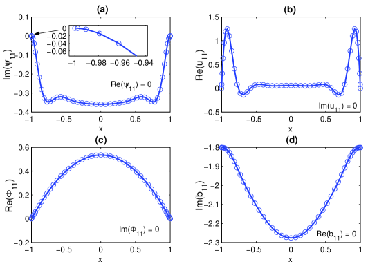
Figure 2: (Color online) Eigenfunctions for the marginal mode at ${\cal C}=0.08$, ${\cal P}_{m}=0.001$, $q=3/2$. Here $Q\sim 0.75$, $R_{{}_{m}}\sim 4.9$. The eigenfunctions are shown fitted (solid line) to the values determined numerically on the Chebyshev grid (open circles). (a) $\Psi_{{}_{11}}$, (b) $u_{{}_{11}}$, (c) $\Phi_{{}_{11}}$, (d) $b_{{}_{11}}$. Note that $Re(\Psi_{{}_{11}})=Im(u_{{}_{11}})=Im(\Phi_{{}_{11}})=Re(b_{{}_{11}})=0$. Because the Prandtl number is small, note rather sharp boundary layers appearing in $\Psi_{{}_{11}}$ and $u_{{}_{11}}$. The inset in (a) resolves the boundary layer behavior near $x=-1$.

IV Weakly Nonlinear Asymptotic Analysis

The weakly nonlinear analysis aims to develop a description of the system’s evolution beginning very close to marginality, slightly into the unstable region. The control parameter in the asymptotic analysis is incorporated in the expression for the background magnetic field. It is here set to be $B_{0}=1-\epsilon^{2}$, i.e. the degree of departure from marginality is controlled by the small parameter $\epsilon$ (of our choosing) whose only formal restriction is that it be $\epsilon\ll 1$.

Close to marginality the relevant MRI mode, discussed in the previous section, may be expressed to leading order in $\epsilon$ (as can be shown by a simple scaling and balancing analysis) in the form

$$\epsilon{\bf V}_{1}\ =\epsilon\left(A\mathbb{V}_{{}_{11}}e^{iQz}+B\mathbb{U}_{{}_{11}}+{\rm c.c}\right),$$

where $\mathbb{V}_{{}_{11}}\equiv(\Psi_{{}_{11}},u_{{}_{11}},\Phi_{{}_{11}},b_{{}_{11}})^{\mathbf{T}}$ and $\mathbb{U}_{{}_{11}}\equiv(0,0,0,1)^{\mathbf{T}}$. The inclusion of $B\mathbb{U}_{{}_{11}}$ in this general solution is dictated by the presence of the neutral mode, discussed at the end of the previous Section.

The weakly nonlinear evolution is asymptotically derived by allowing the amplitudes $A$ and $B$ to be (weakly) dependent on space and time. The aim is to develop an evolution equation for the envelopes $A$ and $B$ (space and time dependent amplitudes) as one tunes the system away from the marginal state defined above at $k=Q$ and ${\cal R}_{m}=R_{m}$. The wisdom garnered from other problems involving cellular instabilities manneville1 ; cross ; manneville2 ; pismen guides us into an Ansatz such that the two envelope functions have functional dependencies upon a long time scale, $T\equiv\epsilon^{2}t$ and a long vertical scale, $Z\equiv\epsilon z$, i.e. we posit the form $A=A(\epsilon^{2}t,\epsilon z),B=B(\epsilon^{2}t,\epsilon z)$. The end-result of this asymptotic procedure, fully detailed in Appendices B and C, are the two (decoupled) amplitude equations

$$\partial_{{}_{T}}A = \lambda A-\alpha A|A|^{2}+D\partial^{2}_{{}_{Z}}A,$$ (18)

$$\partial_{{}_{T}}B = \left(\frac{1}{R_{{}_{m}}}+\frac{{\cal C}{\cal R}}{3}\right)\partial^{2}_{{}_{Z}}B,$$ (19)

where $T\equiv\epsilon^{2}t$, $Z\equiv\epsilon z$ and the coefficients are defined in Appendix B.

We stress here that the decoupling of these two equations is the result of translational ($x$-) symmetry of the thin-gap problem, but it cannot be guaranteed for a case in which, e.g., curvature terms have to be retained. Eq. (19) is the diffusion equation and its physical implications are quite trivial. It indicates that the contribution of the above mentioned neutral mode to the azimuthal field perturbation will simply decay on a time-scale associated with the system’s size and the smaller of either $R_{m}$ or $1/{\cal C}{\cal R}$ - the meaning of the latter possibility will be explored in a forthcoming work. In contrast, equation (18) is the well-studied real Ginzburg-Landau equation (see, e.g. cross ; manneville2 ; pismen ) which can exhibit non-trivial behavior in both the amplitude and phase of the envelope function $A$. The phase can lead to interesting dynamics emerging from Eckhaus-like instabilities, however in the present study we care only about the behavior of the amplitude’s magnitude, i.e. the modulus of A. We shall thus agree henceforth to mean $|A|$, when writing $A$. Further discussion on phase dynamics can be found in the concluding section of this paper.

A real amplitude $A$ in the real GLE has two stable spatially uniform steady solutions, $A(Z,T)=\pm A_{s}$, and one possibly unstable solution, $A=0$, as can be easily verified. Depending on the boundary conditions, the system typically relaxes to one of the steady solutions or, possibly, splits into two regions (the plus and minus values of $A_{s}$) with a front separating them (see e.g., regev for an example of a system of this kind).

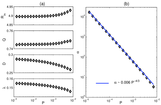
Figure 3: (Color online) Coefficients, parameters and saturation amplitude squared, as a function of ${\cal P}_{m}$, for $q=3/2$, ${\cal C}=0.08$. (a) Plots of $R_{m}$, $Q$, $D$, $\lambda$ as a function of ${\cal P}_{m}$. Note the weak sensitivity on ${\cal P}_{m}$. (b) Values of $\alpha$ (diamonds) as a function of ${\cal P}_{m}$. Plotted as well is the functional dependence $\alpha\sim{\cal P}_{m}^{-4/3}$ (solid line) discussed in the text.

From (18) it is apparent that the saturation amplitude is $A_{s}=\sqrt{\lambda/\alpha}$ and thus its determination calls for the computation of the relevant coefficients. As discussed before this has to be done numerically. The details of this calculation are given in Appendix B and some representative results (for the parameter values $q=3/2$ and ${\cal C}=0.08$) are displayed in Figure 3. Panel (a) demonstrates the weak dependence of $R_{m}$ and $Q$, and of the coefficients $\lambda$ and $D$, on ${\cal P}_{m}$ (for ${\cal P}_{m}\ll 1$). In contrast, the coefficient $\alpha$, whose numerical values are shown in panel (b), has a power law dependence on ${\cal P}_{m}$ in the same interval. Thus, the dependence of the saturation amplitude on ${\cal P}_{m}$ is essentially governed by $\alpha$. The appropriate scaling for ${\cal P}_{m}\ll 1$ is $A_{s}^{2}=\lambda/\alpha\sim 1/\alpha$ (given the very weak dependence of $\lambda$ on ${\cal P}_{m}$).

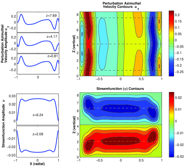
Figure 4: (Color online) Contours of the perturbation streamfunction $(\Psi)$ and azimuthal velocity $(u_{y})$ in the $x-z$ plane, up to and including order $\epsilon^{2}$. The vertical scale of the plots corresponds to one critical wavelength, $2\pi/Q$. The parameters are ${\cal P}_{m}=0.001$, ${\cal C}=0.08$, $\rm R_{m}=4.9$ with $q=3/2$. We take $\epsilon=0.5$ and the amplitude $A=0.07$ (which is its saturation value for this case). Cuts along constant values of $z$ are shown in the left panel (and dashed lines in the contour plots on the right ). Note that $u_{y}$ is the velocity disturbance about the steady profile $-qx$.

The analysis sketched out in Appendix D shows that the dominant terms in the expression for $\alpha$ are such that $\alpha\sim{\cal P}_{m}^{-4/3}$, for ${\cal P}_{m}\ll 1$ This scaling fits very well the numerical results in Figure 3b (solid line). We thus obtain the following scaling behavior for the square of the saturation amplitude

$$A_{s}^{2}\sim{\cal P}_{m}^{4/3}~{}({\rm or}~{}~{}A_{s}^{2}\sim{\cal R}^{-4/3}~{}{\rm for~{}fixed}~{}R_{m}),\qquad{\rm both~{}for}\ \ {\cal P}_{m}\ll 1.$$ (20)

The physical effects that these dominant terms are reflecting can be traced in the asymptotic analysis as resulting from the nonlinear radial advection of the second order azimuthal velocities $u_{x1}\partial_{x}u_{y2}$ and the creation of the azimuthal field due to the shearing of the radial perturbation field $b_{x1}\partial_{x}u_{y2}$. Note that in UMR06 we were able to obtain (from not fully consistent boundary conditions for this problem) the analytical result $A_{s}^{2}\sim{\cal P}_{m}$ (or $\sim{\cal R}^{-1}$ for fixed $R_{m}$). Thus we see that the implementation of more realistic boundary conditions that are appropriate for the thin-gap mTC problem does not alter the general qualitative trend - saturation amplitude increasing with ${\cal P}_{m}$ (or decreasing with $\cal R$ for fixed $R_{m}$) - uncovered in UMR06, nor its implications. It merely alters (slightly) the power of this basic dependence.

In Figure 4 we plot the azimuthal velocity $u_{y}(x,z)$ and the streamfunction $\Psi(x,z)$ of the perturbation, calculated by our asymptotics to order $\epsilon^{2}$. This has to be understood as the modification on top of the basic mTC configuration, which together constitute the steady saturated state. The presence of boundary layers near the channel walls is clearly apparent. In Appendix A we estimate that the boundary layer sizes scale as $\sim{\cal P}_{m}^{1/3}$ and this is quantitatively consistent with the increase in power of the scaling from $A_{s}^{2}\sim{\cal P}_{m}$ (as found in UMR06, where the boundary layers were essentially neglected) to $A_{s}^{2}\sim{\cal P}_{m}^{4/3}$ here. The crucial ingredient in determining the scaling of $A_{s}$ is, as we have seen, the scaling behavior of the coefficient $\alpha$, which in turn is affected by the boundary layer width through its dependence on the relevant $x$-eigenfunctions (see Appendices A and D).

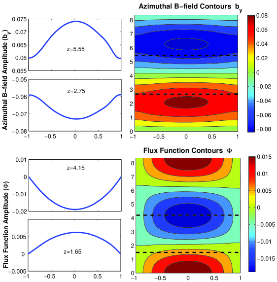
Figure 5: (Color online) Same as Fig. 4 for the azimuthal field (top panels), $b_{y}$, and the flux function, $\Phi$ (bottom panels).

In Figure 5 we display the perturbation’s azimuthal field, $b_{y}$, and its poloidal flux function, $\Phi(x,z)$, in a manner similar to the previous figure. Note that we do not see prominent boundary layers in the magnetic field perturbation; this is the result of the boundary conditions imposed (17). Whereas three velocity boundary conditions are imposed on each side (ensuring zero perturbation velocity on the boundary), only two such conditions on the magnetic field perturbation are enforced ($b_{x}=0,\partial_{x}b_{y}=0$). It is so because precisely ten conditions in all are required, otherwise the problem would be ill-posed.

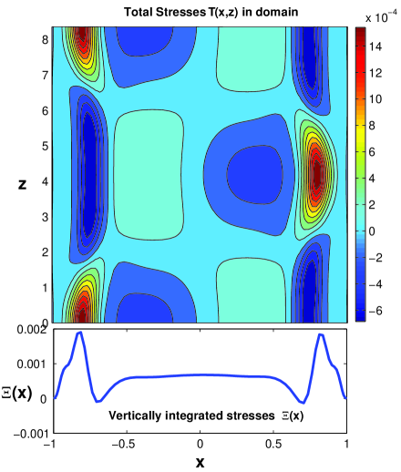
Figure 6: (Color online) Same as Fig. 4 for the total stress, ${\mathbb{T}}(x,z)$ (top panel), and the vertically integrated stress, $\Xi=\int{\mathbb{T}}(x,z)dz$ (bottom panel).

Finally, we turn to the evaluation of the angular momentum transport (a key question in assessing the MRI’s role as the driver of accretion in astrophysical systems). The total (local) stress resulting from the perturbation is composed of the Reynolds and Maxwell stresses and, in our notation, has the form (see, e.g., B03 ,pesahMN , UMR06)

$$\mathbb{T}(x,z)\equiv\mathbb{T}_{\rm R}+\mathbb{T}_{\rm M}=u_{x}u_{y}-{\cal C}b_{x}b_{y}.$$ (21)

As in UMR06, we may define a quantity measuring the average total angular momentum transport in the domain,

$${\mathbf{\dot{J}}}=\frac{Q}{4\pi}\int_{-\pi/Q}^{\pi/Q}dz\left[\int_{-1}^{1}\mathbb{T}(x,z)dx\right].$$

The quantity ${\mathbf{\dot{J}}}$ can be thought of as analogous to similarly defined quantities used as a measure of the effective viscosity parameter due to dynamical fluctuations in active fluid media (for a recent purely hydrodynamic example, see longaretti2 ) - be it either in a fully turbulent state or otherwise. In our problem, this quantity in the saturated state can be written to leading order as

$${\mathbf{\dot{J}}}=\epsilon^{2}|A|^{2}\dot{J}_{0}+{\cal O}\left({\epsilon^{4}}\right),$$ (22)

where $\dot{J}_{0}=\dot{J}_{0}(R_{m},Q;{\cal C},q)$ is of order unity. Given the behavior of the saturated amplitude in the ${\cal P}_{m}\ll 1$ limit, it follows that the average angular momentum transport scales like

$${\mathbf{\dot{J}}}\sim\epsilon^{2}{\cal P}_{m}^{4/3}~{}~{}({\rm or}~{}\sim\epsilon^{2}{\cal R}^{-4/3}~{}{\rm for~{}fixed}~{}R_{m}~{}{\rm of}~{}{\cal O}\left({1}\right)),$$ (23)

to leading order. Finally, we show in Figure 5 the distributed stress $\mathbb{T}(x,y)$ over the domain and the vertically integrated stress, defined by $\Xi(x)\equiv\int\mathbb{T}dz$.

V Discussion and summary

In this paper we have presented a full exposition of a weakly nonlinear asymptotic analysis of the MRI for a viscous and resistive flow in the thin-gap magnetic Taylor-Couette configuration. Our previous work (UMR06) employed mathematically expedient, but not fully consistent boundary conditions for this problem, so as to allow for transparent analytical evaluation of the envelope equation coefficients. Here we have used consistent and realistic boundary conditions for the mTC setup. As a result, the calculation is more involved. We have nevertheless found (as anticipated in UMR06) that in the thin gap limit the amplitude of the disturbances saturates at a value that decreases with decreasing magnetic Prandtl number, ${\cal P}_{m}$. Moreover, the emergence of boundary layers actually makes the ${\cal P}_{m}$-dependence of the saturation amplitude, and thus the average angular momentum transport more severe.

Our results should be put in the proper context. They are valid close to instability threshold and in a confined system (mTC). Most previous studies of the MRI in the nonlinear regime (both numerical and analytical) followed the evolution of channel modes - exponentially growing, radially independent modes (see BHrev ), which happen also to be exact solutions of the nonlinear equations for the perturbation, in the SB formulation under periodic boundary conditions, i.e. in an open system. It is thus only natural that the channel modes have been identified as the dominant dynamics and their evolution perceived as a crucial ingredient in the nonlinear saturation of the instability. Goodman & Xu GX showed that the channel modes ultimately become unstable and break up. The asymptotic study of nonlinear saturation performed by Knobloch & Julien knobloch was also based on a state dominated by channel modes. In these works, as well as the recent local modeling of MRI angular momentum transport pesahMN ; pesahPRL , results were compared with numerical simulations of an open SB (undoubtedly dominated by dynamics arising from the nonlinear evolution of channel modes). Note, however, that in the global approach of Kersalé et al. kersale1 ; kersale2 , the explicit inclusion of boundary conditions and curvature terms broke the radial symmetry of the problem (which is necessary for the channel modes to be manifested). These authors found numerically (using a spectral code) that the form of the saturated state critically depends on the boundary conditions adopted and, in any case, is not a “trivial” Keplerian state with developed MHD turbulence on top of it.

From the vantage point of the linear theory followed here (as well as the SB investigations of the past), the MRI takes place primarily because the term supplying the tension, i.e. a perturbed azimuthal $B$-field, arises from the sheared conversion (by the background flow) of a perturbed radial magnetic field, emanating from the bending of the background vertical field. The strength of the resulting destabilizing torque is related to the magnitude of $q$ (measuring the local stretching) and the magnitude (squared) of the global vertical $B$-field (representing that basic source of tension which is being stretched by the shear). Nonlinear saturation of a linear instability can generically be achieved by increased dissipation, by the modification of the linearly unstable base state so as to push it back to stability, or a combination of both.

In the problem studied here, we have considered the marginal MRI mode (i.e. with growth rate 0), as a function of all free parameters, save $q$, which has been fixed to 3/2. We find that the saturated azimuthal velocity disturbance provides an effective positive radial gradient, $q^{\prime}>0$, through the bulk of the flow (see Figure 4). Thus the effective overall $q$ in the saturated state is $q_{\rm eff}=q-q^{\prime}<3/2$. The magnitude of the effective gradient reflects the manner in which the modified gradient couples to the background field which is being stretched and is responsible for the instability. In our case, $q^{\prime}$ is positive and thus reduces the initial destabilizing shear, but not sufficiently to cancel it entirely. It has to be noted, however, that the saturated state is not just the base flow with reduced shear. It includes also extra poloidal and azimuthal field, as well as poloidal velocity. This steady state is thus more complicated; the presence of velocity boundary layers complicates it even further. It is thus not trivial to identify a simple process for the saturation ”mechanism” in this case. We note that our results share similarities with the saturation mechanism proposed by Knobloch & Julien knobloch for the saturated MRI state developed, in a particular asymptotic regime, from the unstable channel modes discussed above.

We have followed into the weakly nonlinear regime a dissipative system, which was in a marginal balance and obtained a steady saturated state from a reduction of the shear, in places over the domain where it counts the most (in terms of azimuthal field production), and from the emergence of a steady flow and magnetic field configuration. In terms of dissipation, it is instructive to consider the energy relationship (15). In our steady saturated state the first integral is just $\propto\int\Xi(x)dx$ and therefore is positive (see the bottom of Fig. 6). As $\partial_{t}E$ in this (steady) saturated state must be zero, the sum of the two dissipative integrals must be equal to the first one. We have verified that it is indeed so.

We have not considered in this paper phase dynamics, which is an inherent feature of the more general envelope in complex GLE. Phase dynamics may be rich, in particular in two and three dimensions, admitting well-known pattern instabilities like Eckhaus and Zig-Zag and these, in turn, can lead to effects like phase turbulence and complicated defect dynamics manneville2 ; pismen . In what is considered here, where the coefficients of the one-dimensional GLE are real, all that remains of the above is just a possibility of an Eckhaus instability. This may merely introduce some non-steady readjustment to the overall pattern phase, but it leaves unaltered the overall amplitude scale of the basic pattern that emerges. In particular, our system is open in the $z$ dimension and thus there should be no difficulty for the phase to adjust itself to a stable value (see manneville2 p. 200). Because we are interested here in the scaling of the transport (which is expressed by an integral of the envelope over the domain), phase dynamics (although interesting in its own right) does not influence this measure and we have thus considered only the modulus of the envelope.

Our results and findings here should ultimately be compared to experiments and numerical simulations accompanying them. Extension of this type of analysis to a wide-gap mTC configuration is possible, but the results will be somewhat more complicated than those presented here, due to the inclusion of curvature terms. Preliminary calculations indicate that the evolution of the perturbation amplitude in this case is governed by two coupled envelope equations (see Appendix B). The properties of the saturated state, however, appear similar in their salient features to the ones explored in this paper. The case of an initial helical field, for which experimental detection of the MRI has recently been reported helical , can also be investigated in the weakly nonlinear asymptotic formalism employed here. It will the subject of future work.

Further analytical investigations of the nonlinear MRI, of the kind reported here, will contribute toward assembling a deeper understanding of this important instability. Such investigations may also help in addressing the issues of the effect of numerical resolution upon the resulting dynamics. In particular it could be useful to conduct simulations for, say, a fixed value of the magnetic Reynolds number (well below any contamination by numerical dissipation) and examine if and how does the transport change with resolution. Numerical studies of the MHD turbulent dynamo problem (e.g., cata ; brand2 ) have shown that such considerations are very important. The understanding of the role that the MRI plays in astrophysical disks, which in its full generality is a formidable problem, may be enriched by the experimental, analytical and numerical studies of simpler systems.

Appendix A The linear scale of the boundary layer

The best way to identify the scalings that are appropriate for the boundary layer is to rewrite (16) as a single equation for, say, the streamfunction $\Psi$. Setting the time-derivative to zero results in

$${\cal L}\Psi=\left\{\left({\cal P}_{m}(D_{x}^{2}-Q^{2})^{2}+{\cal C}R_{m}^{2}Q^{2}\right)^{2}(D_{x}^{2}-Q^{2})+R_{m}^{4}2q{\cal C}Q^{4}-\omega_{e}^{2}Q^{2}(D_{x}^{2}-Q^{2})^{2}{R_{m}^{2}}\right\}\Psi=0,$$ (24)

where $\omega_{e}^{2}\equiv 2(2-q)$ and where the simplifying notation $D_{x}\equiv d/dx$ is also used. The operator is tenth order in $D_{x}$ derivatives. Inspection of its form suggests that retaining only the terms of (24) that are dominant (for ${\cal P}_{m}\ll 1$) in a small region of size $~{}{\cal P}_{m}^{\lambda}$ with $\lambda>0$ (the total $x$-domain size is 2 in our units) at either of the two boundaries gives

$$\left({\cal P}_{m}^{2}D_{x}^{10}-\omega_{e}^{2}Q^{2}D_{x}^{4}{R_{m}^{2}}\right)\Psi=0.$$ (25)

Treating all quantities as being of ${\cal O}\left({1}\right)$ except for ${\cal P}_{m}$, we can now see that the value of the exponent $\lambda$ must be $1/3$. More explicitly, we consider a boundary layer by rescaling the x-coordinate around the boundaries at $x=\pm 1$. We define $\xi\equiv{\cal P}_{m}^{-\lambda}(x\mp 1)$ and insert this into (24) revealing

$$\left({\cal P}_{m}^{2-10\lambda}D_{\xi}^{10}-{\cal P}_{m}^{-4\lambda}\omega_{e}^{2}Q^{2}{R_{m}^{2}}D_{\xi}^{4}\right)\Psi+{\cal O}\left({{\cal P}_{m}^{2-8\lambda},\cdots,1}\right)=0,$$ (26)

where $D_{\xi}\equiv d/d\xi$. As ${\cal P}_{m}\rightarrow 0$, a distinguished balancing limit (see, e.g. bender ) may be achieved when $2-10\lambda=-4\lambda$, or when $\lambda=1/3$. In this case, all other terms in the boundary layer region are sub-dominant to the two terms remaining. Thus, in the limit ${\cal P}_{m}\ll 1$, the size of the boundary layer scales as ${\cal P}_{m}^{1/3}$.

Appendix B Derivation of the Ginzburg-Landau Equation

To help facilitate the development of the weakly nonlinear theory we rewrite the equations of motion in the following way,

$${\bf{\cal D}}\partial_{t}{\bf V}+{\bf N}={\bf{\cal L}}{\bf V}+\epsilon^{2}{\bf{\cal G}}{\bf{V}},$$ (27)

in which

$${\bf{\cal L}}\equiv{\bf{L}_{0}}+{\bf{L}_{1}}\partial_{z}+{\bf{L}_{2}}\partial_{z}^{2}+{\bf{L}_{3}}\partial_{z}^{3}+{\bf{L}_{4}}\partial_{z}^{4},$$ (28)

and where the matrices are defined as

$${\bf{L}_{0}} = \left(\begin{array}[]{cccc}{\cal R}^{-1}\partial_{x}^{4}&0&0&0\\ 0&{\cal R}^{-1}\partial_{x}^{2}&0&0\\ 0&0&{\cal R}_{m}^{-1}\partial_{x}^{2}&0\\ 0&0&0&{\cal R}_{m}^{-1}\partial_{x}^{2}\end{array}\right),\qquad{\bf{\cal D}}=\left(\begin{array}[]{cccc}\partial_{x}^{2}+\partial_{z}^{2}&0&0&0\\ 0&1&0&0\\ 0&0&1&0\\ 0&0&0&1\end{array}\right),$$ (37)

$${\bf{L}_{1}} = \left(\begin{array}[]{cccc}0&2&{\cal C}\partial_{x}^{2}&0\\ 2-q&0&0&{\cal C}\\ 1&0&0&0\\ 0&1&-q&0\end{array}\right),\qquad{\bf{L}_{2}}=\left(\begin{array}[]{cccc}2{\cal R}^{-1}\partial_{x}^{2}&0&0&0\\ 0&{\cal R}^{-1}&0&0\\ 0&0&{\cal R}_{m}^{-1}&0\\ 0&0&0&{\cal R}_{m}^{-1}\end{array}\right),$$ (46)

$${\bf{L}_{3}} = \left(\begin{array}[]{cccc}0&0&{\cal C}&0\\ 0&0&0&0\\ 0&0&0&0\\ 0&0&0&0\end{array}\right),\qquad{\bf{L}_{4}}=\left(\begin{array}[]{cccc}{\cal R}^{-1}&0&0&0\\ 0&0&0&0\\ 0&0&0&0\\ 0&0&0&0\end{array}\right),\qquad{\bf{\cal G}}=\left(\begin{array}[]{cccc}0&0&{\cal C}\partial_{x}^{2}&0\\ 0&0&0&{\cal C}\\ 1&0&0&0\\ 0&1&0&0\end{array}\right).$$ (59)

At marginality, the background vertical field $B_{0}=1$. The degree of linear instability is thus governed by the small parameter $\epsilon$ defined by

$$\epsilon^{2}\equiv 1-B_{0}.$$ (60)

The vectors above are defined by

$${\bf V}\equiv(\Psi,u,\Phi,b)^{\mathbf{{T}}},\qquad{\bf N}\equiv(N_{\Psi},N_{u},N_{\Phi},N_{b})^{\mathbf{T}}.$$

We assume that during the nonlinear development there are two vertical scales emerging in the problem, namely $z$ and $Z\equiv\epsilon z$. We also assume that as one tunes the vertical field parameter $\epsilon^{2}$ into the MRI unstable state, the temporal response scales similarly to $\epsilon^{2}$. Thus we say, for example for the streamfunction, that $\Psi=\Psi(z,\epsilon z,\epsilon^{2}t)$, and similarly for the other physical variables. If we assume that the solution forms follows ${\bf V}={\bf V}(x,z,Z,T)$, then all operators in (27) are re-expressed by applying the replacements

$$\partial_{z}\longrightarrow\partial_{z}+\epsilon\partial_{{}_{Z}},\qquad\partial_{t}\longrightarrow\epsilon^{2}\partial_{{}_{T}}.$$ (61)

Thus, we now have

$$\epsilon^{2}{\mathbf{{\cal D}}}\,\partial_{{}_{T}}{\mathbf{V}}+{\mathbf{N}}={\cal L}{\mathbf{V}}+\epsilon\mathbf{\tilde{{\cal L}}_{1}}\partial_{{}_{Z}}{\mathbf{V}}+\epsilon^{2}\mathbf{\tilde{{\cal L}}_{2}}\partial^{2}_{{}_{Z}}{\mathbf{V}}+\epsilon^{2}\mathbf{\tilde{{\cal G}}}{\mathbf{V}}+{\cal O}\left({\epsilon^{3}}\right),$$ (62)

where

$$\mathbf{\tilde{{\cal L}}_{1}} = {\bf{L}_{1}}+2{\bf{L}_{2}}\partial_{z}+3{\bf{L}_{3}}\partial_{z}^{2}+4{\bf{L}_{4}}\partial_{z}^{3},$$ (63)

$$\mathbf{\tilde{{\cal L}}_{2}} = 2{\bf{L}_{2}}+6{\bf{L}_{3}}\partial_{z}+12{\bf{L}_{4}}\partial_{z}^{2}.$$ (64)

The boundary conditions, aside from periodicity in the vertical, are

$$\partial_{z}\Psi=\partial_{x}\Psi=u_{y}=\partial_{z}\Phi=\partial_{x}b_{y}=0,\qquad{\rm at}\ \ x=\pm 1.$$ (65)

We expand all quantities in a perturbation series

$$\Phi = \epsilon\Phi_{1}+\epsilon^{2}\Phi_{2}+\epsilon^{2}\Phi_{3}+\cdots$$

$$\Psi = \epsilon\Psi_{1}+\epsilon^{2}\Psi_{2}+\epsilon^{2}\Psi_{3}+\cdots$$

$$u_{y} = \epsilon u_{1}+\epsilon^{2}u_{2}+\epsilon^{3}u_{3}+\cdots$$

$$b_{y} = \epsilon b_{1}+\epsilon^{2}b_{2}+\epsilon^{3}b_{3}+\cdots$$

or in other words

$${\mathbf{V}}=\epsilon{\mathbf{V}}_{1}+\epsilon^{2}{\mathbf{V}}_{2}+\epsilon^{3}{\mathbf{V}}_{3}+{\cal O}\left({\epsilon^{4}}\right).$$

With the above expansion and multiple scaling Ansatz, it follows that the nonlinear terms are expressed in the series

$${\mathbf{N}}=\epsilon^{2}{\mathbf{N}_{2}}+\epsilon^{3}{\mathbf{N}_{3}}+{\cal O}\left({\epsilon^{4}}\right),$$ (66)

in which ${\mathbf{N}}=(N^{(\Psi)},N^{(u)},N^{(\Phi)},N^{(b)})^{\mathbf{T}}$. In component by component form, these expressions are explicitly given by

$$N^{(\Psi)} = \epsilon^{2}N^{(\Psi)}_{2}+\epsilon^{3}N^{(\Psi)}_{3}+{\cal O}\left({\epsilon^{4}}\right)$$ (67)

$$N^{(u)} = \epsilon^{2}N^{(u)}_{2}+\epsilon^{3}N^{(u)}_{3}+{\cal O}\left({\epsilon^{4}}\right)$$ (68)

$$N^{(\Phi)} = \epsilon^{2}N^{(\Phi)}_{2}+\epsilon^{3}N^{(\Phi)}_{3}+{\cal O}\left({\epsilon^{4}}\right)$$ (69)

$$N^{(b)} = \epsilon^{2}N^{(b)}_{2}+\epsilon^{3}N^{(b)}_{3}+{\cal O}\left({\epsilon^{4}}\right)$$ (70)

where

$$N^{(\Psi)}_{2} = J(\Psi_{1},\nabla^{2}\Psi_{1})-{\cal C}J(\Phi_{1},\nabla^{2}\Phi_{1})$$ (71)

$$N^{(u)}_{2} = J(\Psi_{1},u_{1})-{\cal C}J(\Phi_{1},b_{1}),$$ (72)

$$N^{(\Phi)}_{2} = -J(\Phi_{1},\Psi_{1}),$$ (73)

$$N^{(b)}_{2} = J(\Psi_{1},b_{1})-J(\Phi_{1},u_{1}),$$ (74)

and

$$N^{(\Psi)}_{3} = J(\Psi_{2},\nabla^{2}\Psi_{1})+J(\Psi_{1},\nabla^{2}\Psi_{2})-{\cal C}J(\Phi_{2},\nabla^{2}\Phi_{1})-{\cal C}J(\Phi_{1},\nabla^{2}\Phi_{2})$$ (75)

$$\tilde{J}(\Psi_{1},\nabla^{2}\Psi_{1})-{\cal C}\tilde{J}(\Phi_{1},\nabla^{2}\Phi_{1})-2J(\Psi_{1},\partial_{z}\partial_{{}_{Z}}\Psi_{1})-2J(\Phi_{1},\partial_{z}\partial_{{}_{Z}}\Phi_{1}),$$

$$N^{(u)}_{3} = J(\Psi_{2},u_{1})+J(\Psi_{1},u_{2})-{\cal C}J(\Phi_{2},b_{1})-{\cal C}J(\Phi_{1},b_{2})-+\tilde{J}(\Psi_{1},u_{1})-{\cal C}\tilde{J}(\Phi_{1},b_{1}),$$ (76)

$$N^{(\Phi)}_{3} = -J(\Phi_{2},\Psi_{1})-J(\Phi_{1},\Psi_{2})-\tilde{J}(\Phi_{1},\Psi_{1}),$$ (77)

$$N^{(b)}_{3} = J(\Psi_{2},b_{1})+J(\Psi_{1},b_{2})-J(\Phi_{2},u_{1})-J(\Phi_{1},u_{2})+\tilde{J}(\Psi_{1},b_{1})-\tilde{J}(\Phi_{1},u_{1}),$$ (78)

in which $\tilde{J}(f,g)\equiv\partial_{{}_{Z}}f\partial_{x}g-\partial_{x}f\partial_{{}_{Z}}g$ (remembering also that $J(f,g)\equiv\partial_{z}f\partial_{x}g-\partial_{x}f\partial_{z}g$).

To ${\cal O}\left({\epsilon}\right)$ we have

$${\cal L}{\mathbf{V}_{{}_{1}}}=0.$$ (79)

The solution to this is the marginal case investigated in the text. We write its general solution form as

$${\mathbf{V}_{{}_{1}}}=A(T,Z)\mathbb{V}_{{}_{11}}e^{iQz}+{{\rm c.c.}}+B(T,Z)\mathbb{U}_{{}_{11}},$$ (80)

where $\mathbb{V}_{{}_{11}}(x)=(\Psi_{{}_{11}},u_{{}_{11}},\Phi_{{}_{11}},b_{{}_{11}})^{\mathbf{T}}$, $\mathbb{U}_{{}_{10}}\equiv(0,0,0,1)^{\mathbf{T}}$ and $A$ and $B$ (not to be confused with the magnetic field) are envelopes (amplitudes). Keeping in mind the above cited solution form, the boundary conditions at this order are

$$\Psi_{{}_{11}}=D_{x}\Psi_{{}_{11}}=u_{{}_{11}}=\Phi_{{}_{11}}=D_{x}b_{{}_{11}}=0,\qquad{\rm at}\ x=\pm 1,$$ (81)

where $D_{x}\equiv d/dx$. Note that the constant azimuthal field symmetry discussed in the main text is embodied in the final term of (80), i.e. $B(T,Z)\mathbb{U}_{{}_{11}}$. We also call attention to the fact that though all of these functions are order 1, they all (especially $u_{{}_{11}}$) show the presence of boundary layers in a region ${\cal O}\left({{\cal P}_{m}^{1/3}}\right)$ close to the two boundaries.

At order $\epsilon^{2}$, the equations are

$${\cal L}{\mathbf{V}_{{}_{2}}}={\mathbf{N}_{2}}-\mathbf{\tilde{{\cal L}}_{1}}\partial_{{}_{Z}}{\mathbf{V}_{{}_{1}}}.$$ (82)

The solution at this order is written as

$${\mathbf{V}_{{}_{2}}}=A^{2}\mathbb{V}_{{}_{22}}e^{i2Qz}+\partial_{{}_{Z}}A\mathbb{V}_{{}_{21}}e^{iQz}+|A|^{2}\mathbb{V}_{{}_{20}}+\partial_{{}_{Z}}B\mathbb{U}_{{}_{20}}+{{\rm c.c.}}$$ (83)

where $\mathbf{V}_{{}_{2}}\equiv(\Psi_{2},u_{2},\Phi_{2},b_{2})^{\mathbf{T}}$ and in particular, $\mathbb{V}_{{}_{22}}(x)\equiv(\Psi_{22},u_{22},\Phi_{22},b_{22})^{\mathbf{T}}$, $\mathbb{V}_{{}_{21}}(x)\equiv(\Psi_{21},u_{21},\Phi_{21},b_{21})^{\mathbf{T}}$, $\mathbb{V}_{{}_{20}}(x)\equiv(\Psi_{20},u_{20},\Phi_{20},b_{20})^{\mathbf{T}}$,and $\mathbb{U}_{{}_{20}}(x)\equiv(0,\tilde{u}_{20},0,0)^{\mathbf{T}}$. ${\mathbf{N}_{2}}$ contains no terms resonant with $e^{iQz}$ (see below) but because the expression $\mathbf{\tilde{{\cal L}}_{1}}\partial_{{}_{Z}}{\mathbf{V}_{{}_{1}}}$ does contain such a term, in order for there to be a bounded solution at this order with the required boundary condition, the following solvability condition (the vanishing of an inner product note_2 ) must be satisfied:

$$\left<{{\mathbf{V}^{\dagger}\cdot\mathbf{\tilde{{\cal L}}_{1}}\partial_{{}_{Z}}{\mathbf{V}_{{}_{1}}}}}\right>\equiv\frac{Q}{2\pi}\int_{{}_{-1}}^{1}\int_{-\pi/Q}^{\pi/Q}dxdz{{\mathbf{V}^{\dagger}\cdot\mathbf{\tilde{{\cal L}}_{1}}\partial_{{}_{Z}}{\mathbf{V}_{{}_{1}}}}}=0,$$ (84)

where ${\mathbf{V}^{\dagger}}$ is the solution to the adjoint operation

$$\mathbf{{\cal L}^{\dagger}}{\mathbf{V}^{\dagger}}=0.$$ (85)

The adjoint operator is given by

$${\mathbf{\cal L}^{\dagger}}\equiv{\mathbf{L}_{0}}-{\mathbf{L}_{1}}^{\mathbf{T}}\partial_{z}+{\mathbf{L}_{2}}\partial_{z}^{2}-{\mathbf{L}_{3}}^{\mathbf{T}}\partial_{z}^{3}+{\mathbf{L}_{4}}\partial_{z}^{4}.$$ (86)

and is so written since

$${\mathbf{L}_{0}}=\left({\mathbf{L}_{0}}\right)^{\mathbf{T}},\quad{\mathbf{L}_{1}}=\left({\mathbf{L}_{2}}\right)^{\mathbf{T}},\quad{\mathbf{L}_{4}}=\left({\mathbf{L}_{3}}\right)^{\mathbf{T}}.$$

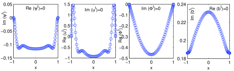
Figure 7: (Color online) The adjoint solution $\mathbb{V}^{\dagger}$ for ${\cal C}=0.08$, ${\cal P}_{m}=0.001$, $q=3/2$ with $R_{{}_{m}}\sim 4.9$ and $Q\sim 0.75$. The open circles are the values on the Chebyshev grid while the solid lines are fits.

The adjoint solution ${\mathbf{V}^{\dagger}}\equiv\mathbb{V}^{\dagger}e^{iQz}+{\rm c.c.}$, in which $\mathbb{V}^{\dagger}\equiv(\Psi^{\dagger},u^{\dagger},\Phi^{\dagger},b^{\dagger})^{\mathbf{T}}$ is such that it satisfies the boundary conditions

$$\Psi^{\dagger}=\partial_{x}\Psi^{\dagger}=u^{\dagger}=\Phi^{\dagger}=\partial_{x}b^{\dagger}=0,\qquad{\rm at}\ \ x=\pm 1,$$ (87)

in addition to periodicity in the vertical direction. In Figure (7), we display an example of $\mathbb{V}^{\dagger}$. We note that it is also an even function with respect to $x$. The solvability condition (84) is automatically satisfied on account of the choice of $Q$ and $R_{m}$, as discussed in the main text. To complete this exposition, we explicitly write out the nonlinear terms appearing in $\mathbf{N_{2}}$,

$$\mathbf{N}_{2}=A^{2}\mathbf{N}_{22}e^{i2Qz}+|A|^{2}\mathbf{N}_{20}+{\rm c.c.,}$$

where $\mathbf{N}_{22}\equiv(N^{(\Psi)}_{{}_{22}},N^{(\Psi)}_{{}_{22}},N^{(\Psi)}_{{}_{22}},N^{(\Psi)}_{{}_{22}})^{\mathbf{T}}$, $\mathbf{N}_{20}\equiv(N^{(\Psi)}_{{}_{20}},N^{(\Psi)}_{{}_{20}},N^{(\Psi)}_{{}_{20}},N^{(\Psi)}_{{}_{20}})^{\mathbf{T}}$ and

$$N^{(\Psi)}_{{}_{22}} = (iQ\Psi_{{}_{11}})\cdot D_{x}(D_{x}^{2}-Q^{2})\Psi_{{}_{11}}-(D_{x}\Psi_{{}_{11}})\cdot iQ(D_{x}^{2}-Q^{2})\Psi_{{}_{11}}$$

$$-{\cal C}\left[(iQ\Phi_{{}_{11}})\cdot D_{x}(D_{x}^{2}-Q^{2})\Phi_{{}_{11}}-(D_{x}\Phi_{{}_{11}})\cdot iQ(D_{x}^{2}-Q^{2})\Phi_{{}_{11}}\right]$$

$$N^{(u)}_{{}_{22}} = (iQ\Psi_{{}_{11}})\cdot D_{x}u_{{}_{11}}-(D_{x}\Psi_{{}_{11}})\cdot iQu_{{}_{11}}-{\cal C}\left[(iQ\Phi_{{}_{11}})\cdot D_{x}b_{{}_{11}}-(D_{x}\Phi_{{}_{11}})\cdot iQb_{{}_{11}}\right]$$

$$N^{(\Phi)}_{{}_{22}} = -\left[(iQ\Phi_{{}_{11}})\cdot D_{x}\Psi_{{}_{11}}-(D_{x}\Phi_{{}_{11}})\cdot iQ\Psi_{{}_{11}}\right]$$

$$N^{(b)}_{{}_{22}} = (iQ\Psi_{{}_{11}})\cdot D_{x}b_{{}_{11}}-(D_{x}\Psi_{{}_{11}})\cdot iQb_{{}_{11}}-{\cal C}\left[(iQ\Phi_{{}_{11}})\cdot D_{x}u_{{}_{11}}-(D_{x}\Phi_{{}_{11}})\cdot iQu_{{}_{11}}\right],$$ (88)

and

$$N^{(\Psi)}_{{}_{20}} = (iQ\Psi_{{}_{11}})\cdot(D_{x}(D_{x}^{2}-Q^{2})\Psi_{{}_{11}})^{*}-(D_{x}\Psi_{{}_{11}})\cdot(iQ(D_{x}^{2}-Q^{2})\Psi_{{}_{11}})^{*}$$

$$-{\cal C}\left[(iQ\Phi_{{}_{11}})\cdot(D_{x}(D_{x}^{2}-Q^{2})\Phi_{{}_{11}})^{*}-(D_{x}\Phi_{{}_{11}})\cdot(iQ(D_{x}^{2}-Q^{2})\Phi_{{}_{11}})^{*}\right]$$

$$N^{(u)}_{{}_{20}} = \underline{(iQ\Psi_{{}_{11}})\cdot(D_{x}u_{{}_{11}})^{*}}-(D_{x}\Psi_{{}_{11}})\cdot(iQu_{{}_{11}})^{*}-\left[(iQ\Phi_{{}_{11}})\cdot(D_{x}b_{{}_{11}})^{*}-(D_{x}\Phi_{{}_{11}})\cdot(iQb_{{}_{11}})^{*}\right]$$

$$N^{(\Phi)}_{{}_{20}} = -\left[(iQ\Phi_{{}_{11}})\cdot(D_{x}\Psi_{{}_{11}})^{*}-(D_{x}\Phi_{{}_{11}})\cdot(iQ\Psi_{{}_{11}})^{*}\right]$$

$$N^{(b)}_{{}_{20}} = (iQ\Psi_{{}_{11}})\cdot(D_{x}b_{{}_{11}})^{*}-(D_{x}\Psi_{{}_{11}})\cdot(iQb_{{}_{11}})^{*}-\left[(iQ\Phi_{{}_{11}})\cdot(D_{x}u_{{}_{11}})^{*}-(D_{x}\Phi_{{}_{11}})\cdot(iQu_{{}_{11}})^{*}\right].$$

Superscript“*” on any given quantity (i.e. $f^{*}$) denotes the complex conjugation of the said quantity. We solve for the quantities $\mathbb{V}_{{}_{22}},\mathbb{V}_{{}_{21}},\mathbb{V}_{{}_{20}}$ using the Chebyshev collocation technique developed for the linear theory and show an example of these results in Figure 8. We note that the functions of $\mathbb{V}_{{}_{22}},\mathbb{V}_{{}_{20}}$ are odd with respect to $x$ while those of $\mathbb{V}_{{}_{21}}$ are even with respect to $x$. We also call attention to the fact that since $N^{(b)}_{20}+\left(N^{(b)}_{20}\right)^{*}=0$, $b_{{}_{20}}$ is also zero. This is significant because it is really a consequence of a second condition that must be met to ensure the existence of a solution at this order. In particular, inspection of the $z$ independent component of the equation describing the evolution of $b_{2}$, i.e.,

$$R_{{}_{m}}^{-1}\partial_{x}^{2}b_{{}_{20}}=|A|^{2}\left[N^{(b)}_{20}+\left(N^{(b)}_{20}\right)^{*}\right],$$ (90)

shows that in order for there to be a solution to $b_{{}_{20}}$, which satisfies the boundary conditions $\partial_{x}b_{{}_{20}}=0$ at $x=\pm 1$, a condition must be met with respect to the terms on the right-hand side of (90). This criterion is most simply seen by (i) integrating this equation from $x=-1$ to $x=1$, (ii) applying boundary conditions, (iii) leaving the requirement

$$0=|A|^{2}\int_{-1}^{1}\left[N^{(b)}_{20}+\left(N^{(b)}_{20}\right)^{*}\right]dx.$$

However, this relationship is automatically satisfied on account of the fact that $Re(N^{(b)}_{20})=0$, as noted above.

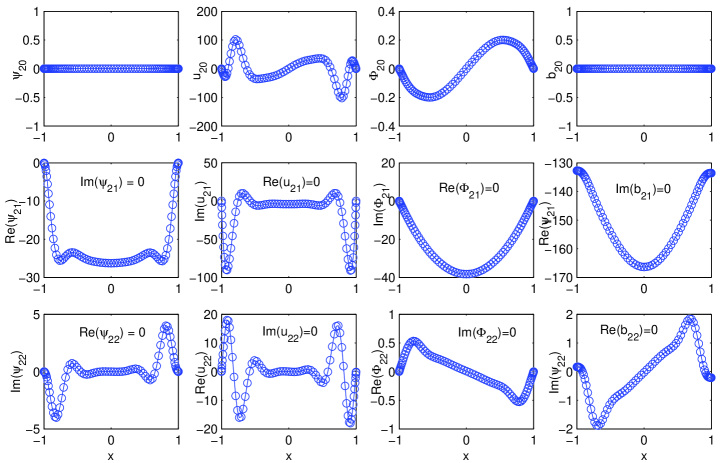
Figure 8: (Color online) The second order solutions $\mathbb{V}_{22},\mathbb{V}_{21},\mathbb{V}_{20}$ for ${\cal C}=0.08$, ${\cal P}_{m}=0.001$, $q=3/2$ with $R_{{}_{m}}\sim 4.9$ and $Q\sim 0.75$. Note the pronounced boundary layers in $u_{22},u_{21}$, $u_{20}$ and, to a lesser degree, $\Psi_{21}$.

We complete the solution to this order by explicitly writing out the form for $\tilde{u}_{20}$ which is associated with $\partial_{Z}B$ - c.f. (83). The equation governing its structure is

$${\cal R}^{-1}\partial_{x}^{2}\tilde{u}_{20}=-{\cal C},$$ (91)

yielding the solution

$$\tilde{u}_{20}=\frac{1}{2}{\cal C}{\cal R}(x^{2}-1).$$ (92)

Finally, at order $\epsilon^{3}$, the equations are

$${\mathbf{{\cal D}}}\partial_{{}_{T}}{\mathbf{V}_{{}_{1}}}+{\mathbf{N}_{3}}={\cal L}{\mathbf{V}_{{}_{3}}}+\mathbf{\tilde{{\cal L}}_{1}}\partial_{{}_{Z}}{\mathbf{V}_{{}_{2}}}+\mathbf{\tilde{{\cal L}}_{2}}\partial^{2}_{{}_{Z}}{\mathbf{V}_{{}_{1}}}+\mathbf{\tilde{{\cal G}}}{\mathbf{V}_{{}_{1}}}.$$ (93)

The terms of the nonlinear functional ${\mathbf{N}_{3}}$ have the more detailed following expansion

$${\mathbf{N}_{3}}=A^{3}\mathbf{N}_{33}e^{i3Qz}+A\partial_{{}_{Z}}A\mathbf{N}_{32}e^{i2Qz}+A|A|^{2}\mathbf{N}_{31}e^{iQz}+A\partial_{{}_{Z}}B\mathbf{\tilde{N}}_{31}e^{iQz}+A^{*}\partial_{{}_{Z}}A\mathbf{N}_{30}+{\rm c.c.}$$ (94)

In order for there to be a solution at this order, the same solvability condition discussed earlier must also be satisfied for this equation. Those terms in the above expression subject to the solvability condition are the ones resonant with $e^{iQz}$ (see the definition of $\mathbf{V}^{\dagger}$ above). Our goal in this work is to satisfy this solvability condition, at this order. In turn, this means that the only two terms from the nonlinear expression that will concern us here with this first solvability (see below) will be the expressions involving $\mathbf{N}_{31}$ and $\mathbf{\tilde{N}}_{31}$. The explicit forms for these expressions are given in Appendix C (in order not to clutter this exposition). The main feature to note about these functions is that $\mathbf{N}_{31}$ is even with respect to $x$ while $\mathbf{\tilde{N}}_{31}$ is odd. The ramifications of these facts are explained below. The solvability condition means taking the inner product of (93) with $\mathbf{V}^{\dagger}$, revealing

$$a\partial_{{}_{T}}A+cA|A|^{2}+\tilde{c}A\partial_{{}_{Z}}B=bA+h\partial^{2}_{{}_{Z}}A,$$ (95)

where

$$a\equiv\left<\mathbb{V}^{\dagger}\cdot{\cal D}\mathbb{V}_{{}_{11}}^{*}\right>,\quad c \equiv \left<\mathbb{V}^{\dagger}\cdot\mathbf{N}_{31}^{*}\right>,\quad\tilde{c}\equiv\left<\mathbb{V}^{\dagger}\cdot\mathbf{\tilde{N}}_{31}^{*}\right>,\quad b\equiv\left<\mathbb{V}^{\dagger}\cdot({\cal G}\mathbb{V}_{{}_{11}})^{*}\right>,$$

$$\quad h \equiv \left<\mathbb{V}^{\dagger}\cdot\left(\mathbf{\tilde{{\cal L}}_{1}}\mathbb{V}_{{}_{21}}+\mathbf{\tilde{{\cal L}}_{2}}\mathbb{V}_{{}_{11}}\right)^{*}\right>.$$ (96)

Inspecting the expressions comprising $\mathbf{\tilde{N}}_{31}$ reveals that they are odd symmetric with respect to $x$. This result means that the expression $\tilde{c}=0$ and, consequently, it means that the evolution equation for the field $A$ evolves according to

$$\partial_{{}_{T}}A=\lambda A+D\partial^{2}_{{}_{Z}}A-\alpha A|A|^{2},\qquad{\rm where}\quad\lambda\equiv b/a,\quad D\equiv h/a,\quad\alpha=c/a,$$ (97)

independent of the second field quantity $B$. This decoupling is a direct consequence of the symmetries preserved in the thin gap Taylor-Couette limit. This will not be the case in the general-gap magnetized Taylor-Couette problem.

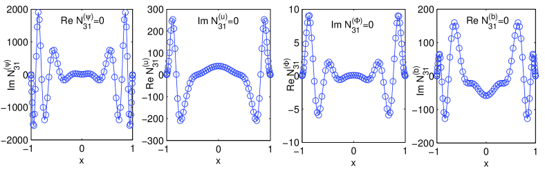
Figure 9: (Color online) The non-linear function $\mathbf{N}_{31}$ for ${\cal C}=0.08$, ${\cal P}_{m}=0.001$, $q=3/2$ with $R_{{}_{m}}\sim 4.9$ and $Q\sim 0.75$.

As noted earlier, there is a second solvability condition, which must be enforced on the order $\epsilon^{3}$ $B$-equation. This becomes necessary on the component of the solution for which there is no explicit $z$ dependence. More explicitly, writing out that component of the equation:

$${R}_{{}_{m}}^{-1}\partial_{x}^{2}b_{30}=\partial_{{}_{T}}B-{R}_{{}_{m}}^{-1}\partial^{2}_{{}_{Z}}B-\tilde{u}_{20}\partial_{{}_{Z}}^{2}B+\Bigl{[}A^{*}\partial_{{}_{Z}}AN^{(b)}_{30}+{\rm c.c.}\Bigr{]}.$$ (98)

The solvability condition can be readily inferred by integrating (98) from $x=-1$ to $x=1$ and requiring that $\partial_{x}b_{30}=0$ at $x=\pm 1$. This procedure is equivalent to taking the inner product of (93) multiplied by $\mathbb{U}_{{}_{11}}$, thus revealing the second envelope equation

$$\partial_{{}_{T}}B=\left(\frac{1}{R_{{}_{m}}}+\frac{{\cal C}{\cal R}}{3}\right)\partial^{2}_{{}_{Z}}B-p\partial_{{}_{Z}}|A^{2}|,$$

where $p\equiv\left<Re\left(N^{(b)}_{30}\right)\right>$. However, the odd symmetry property of $N^{(b)}_{30}$ means that $p=0$. Thus, the second solvability condition yields the simple diffusion equation,

$$\partial_{{}_{T}}B=\left(\frac{1}{R_{{}_{m}}}+\frac{{\cal C}{\cal R}}{3}\right)\partial^{2}_{{}_{Z}}B.$$ (99)

Appendix C The terms for $\mathbf{N}_{31}$

We define for notational convenience the symbols $\nabla_{1}^{2}\equiv D_{x}^{2}-Q^{2}$ and $\nabla_{2}^{2}\equiv D_{x}^{2}-4Q^{2}$. It follows that the expressions are

$$N^{(\Psi)}_{{}_{31}} = (i2Q\Psi_{{}_{22}})(D_{x}\nabla_{1}^{2}\Psi_{{}_{11}})^{*}-\left[(D_{x}\Psi_{{}_{22}})\cdot(iQ\nabla_{1}^{2}\Psi_{{}_{11}})^{*}+(D_{x}\Psi_{{}_{20}})\cdot(iQ\nabla_{1}^{2}\Psi_{{}_{11}})\right]$$ (100)

$$+(iQ\Psi_{{}_{11}})^{*}\cdot(D_{x}\nabla_{2}^{2}\Psi_{{}_{22}})+(iQ\Psi_{{}_{11}})\cdot D_{x}D_{x}^{2}\Psi_{{}_{20}}-(D_{x}\Psi_{{}_{11}})^{*}\cdot(i2Q\nabla_{2}^{2}\Psi_{{}_{22}})$$

$$-{\cal C}\left\{(i2Q\Phi_{{}_{22}})(D_{x}\nabla_{1}^{2}\Phi_{{}_{11}})^{*}-\left[(D_{x}\Phi_{{}_{22}})\cdot(iQ\nabla_{1}^{2}\Phi_{{}_{11}})^{*}+(D_{x}\Phi_{{}_{20}})\cdot(iQ\nabla_{1}^{2}\Phi_{{}_{11}})\right]\right\}$$

$$-{\cal C}\left\{(iQ\Phi_{{}_{11}})^{*}\cdot(D_{x}\nabla_{2}^{2}\Phi_{{}_{22}})+(iQ\Phi_{{}_{11}})\cdot D_{x}D_{x}^{2}\Phi_{{}_{20}}-(D_{x}\Phi_{{}_{11}})^{*}\cdot(i2Q\nabla_{2}^{2}\Phi_{{}_{22}})\right\},$$

$$N^{(u)}_{{}_{31}} = (i2Q\Psi_{{}_{22}})(D_{x}u_{{}_{11}})^{*}-\left[(D_{x}\Psi_{{}_{22}})\cdot(iQu_{{}_{11}})^{*}+(D_{x}\Psi_{{}_{20}})\cdot(iQu_{{}_{11}})\right]$$ (101)

$$+(iQ\Psi_{{}_{11}})^{*}\cdot(D_{x}u_{{}_{22}})+\underline{(iQ\Psi_{{}_{11}})\cdot D_{x}u_{{}_{20}}}-(D_{x}\Psi_{{}_{11}})^{*}\cdot(i2Qu_{{}_{22}})$$

$$-{\cal C}\left\{(i2Q\Phi_{{}_{22}})(D_{x}b_{{}_{11}})^{*}-\left[(D_{x}\Phi_{{}_{22}})\cdot(iQb_{{}_{11}})^{*}+(D_{x}\Phi_{{}_{20}})\cdot(iQb_{{}_{11}})\right]\right\}$$

$$-{\cal C}\left\{(iQ\Phi_{{}_{11}})^{*}\cdot(D_{x}b_{{}_{22}})+(iQ\Phi_{{}_{11}})\cdot D_{x}b_{{}_{20}}-(D_{x}\Phi_{{}_{11}})^{*}\cdot(i2Qb_{{}_{22}})\right\},$$

$$N^{(\Phi)}_{{}_{31}} = -\left\{(i2Q\Psi_{{}_{22}})(D_{x}\Psi_{{}_{11}})^{*}-\left[(D_{x}\Psi_{{}_{22}})\cdot(iQ\Psi_{{}_{11}})^{*}+(D_{x}\Psi_{{}_{20}})\cdot(iQu\Psi_{{}_{11}})\right]\right\}$$ (102)

$$\left\{(iQ\Psi_{{}_{11}})^{*}\cdot(D_{x}\Psi_{{}_{22}})+(iQ\Psi_{{}_{11}})\cdot D_{x}\Psi_{{}_{20}}-(D_{x}\Psi_{{}_{11}})^{*}\cdot(i2Q\Psi_{{}_{22}})\right\},$$

$$N^{(b)}_{{}_{31}} = (i2Q\Psi_{{}_{22}})(D_{x}b_{{}_{11}})^{*}-\left[(D_{x}\Psi_{{}_{22}})\cdot(iQb_{{}_{11}})^{*}+(D_{x}\Psi_{{}_{20}})\cdot(iQb_{{}_{11}})\right]$$ (103)

$$+(iQ\Psi_{{}_{11}})^{*}\cdot(D_{x}b_{{}_{22}})+(iQ\Psi_{{}_{11}})\cdot D_{x}b_{{}_{20}}-(D_{x}\Psi_{{}_{11}})^{*}\cdot(i2Qb_{{}_{22}})$$

$$-\left\{(i2Q\Phi_{{}_{22}})(D_{x}u_{{}_{11}})^{*}-\left[(D_{x}\Phi_{{}_{22}})\cdot(iQu_{{}_{11}})^{*}+(D_{x}\Phi_{{}_{20}})\cdot(iQu_{{}_{11}})\right]\right\}$$

$$-\left\{(iQ\Phi_{{}_{11}})^{*}\cdot(D_{x}u_{{}_{22}})+\underline{(iQ\Phi_{{}_{11}})\cdot D_{x}u_{{}_{20}}}-(D_{x}\Phi_{{}_{11}})^{*}\cdot(i2Qu_{{}_{22}})\right\}$$

and

$$\tilde{N}^{(\Psi)}_{{}_{31}} = 0$$ (104)

$$\tilde{N}^{(u)}_{{}_{31}} = (iQ\Psi_{{}_{11}})\cdot D_{x}\tilde{u}_{{}_{20}}$$ (105)

$$\tilde{N}^{(\Phi)}_{{}_{31}} = 0$$ (106)

$$\tilde{N}^{(b)}_{{}_{31}} = -(iQ\Phi_{{}_{11}})\cdot D_{x}\tilde{u}_{{}_{20}}$$ (107)

Appendix D On the ${\cal O}\left({{\cal P}_{m}^{-4/3}}\right)$ dependence of $\alpha$.

There are a number of terms comprising the integral expression leading to the quantity $\alpha$. Of these, there are a few that dominate its expression when ${\cal P}_{m}$ is small. In the following, we will sketch out one way to understand the ${\cal O}\left({{\cal P}_{m}^{-4/3}}\right)$ scaling behavior of $\alpha$. (Note that because we consider the behavior of this system by holding ${\cal R}_{m}={\rm R}_{m}$ fixed, we will speak about the general scaling dependencies of quantities on ${\cal P}_{m}$ and ${\cal R}^{-1}$ interchangeably as they are, in effect, equivalent under this constraint.)

We noted earlier that the lowest order functions comprising $\mathbb{V}_{{}_{11}}$ exhibit boundary layers of spatial extent ${\cal O}\left({{\cal P}_{m}^{1/3}}\right)$ for ${\cal P}_{m}\ll 1$. Especially acute in this respect is the function for the azimuthal velocity perturbation, $u_{{}_{11}}$. At the next order, we find that the equation for $u_{{}_{20}}$ (i.e. the second order azimuthal velocity function with no dependence on the $z$ coordinate) is simply

$${\cal R}^{{}^{-1}}\partial_{x}^{2}u_{{}_{20}}=N^{(u)}_{{}_{20}}.$$ (108)

Inspection of (LABEL:N20_expressions) shows that $N^{(u)}_{{}_{20}}$ is dominated by the underlined term containing the expression $D_{x}u_{{}_{11}}$. (Note that it is true that the other quantities also, in principle, have boundary layers as well but the one associated with $D_{x}u_{{}_{11}}$ dominates - inspection of Fig. 2 readily shows.) This means that in the boundary layer regions, $N^{(u)}_{{}_{20}}$ scales as ${\cal O}\left({{\cal P}_{m}^{-1/3}}\right)$ while in the interior it remains ${\cal O}\left({1}\right)$. It follows from inspection of (108) that $u_{{}_{20}}$ scales as ${\cal O}\left({{\cal P}_{m}^{-4/3}}\right)$ in the boundary layers and ${\cal O}\left({{\cal P}_{m}^{-1}}\right)$ in the bulk interior.

Now we turn to an inspection of the expression leading to $\alpha$, namely term $c$ of (96) which is composed, in part, of the integrals over the domain of the products $u^{\dagger}\cdot N^{(u)}_{{}_{31}}$ and $b^{\dagger}\cdot N^{(b)}_{{}_{31}}$. Since $u^{\dagger}$ and $b^{\dagger}$ remain ${\cal O}\left({1}\right)$ over the entirety of the domain, it remains for us to evaluate the behavior of $N^{(u)}_{{}_{31}}$ and $N^{(b)}_{{}_{31}}$ over the domain. Although there are several terms that contribute, one of the terms is most dominant: the underlined expressions in (101), which involves $D_{x}u_{{}_{20}}$. Because there is a derivative, the scale of $D_{x}u_{{}_{20}}$ gets amplified by another factor of ${\cal P}_{m}^{-1/3}$ in the boundary layer region. Given what we have established thus far about the character and profile of $u_{{}_{20}}$, it follows that $D_{x}u_{{}_{20}}$ is ${\cal O}\left({{\cal P}_{m}^{-5/3}}\right)$ in the boundary layer regions while it is ${\cal O}\left({{\cal P}_{m}^{-1}}\right)$ in the interior. It means, therefore, that the profiles of $N^{(u)}_{{}_{31}}$ and $N^{(b)}_{{}_{31}}$ similarly reflect this character on the $x$ domain.

Thus, for instance, to determine the order of magnitude of the integral of $b^{\dagger}N^{(b)}_{{}_{31}}$ over the domain, we should break up the integral into parts separating out the interior region and boundary layers. Writing $\delta={\cal P}_{m}^{1/3}$ we have

$$\int_{-1}^{1}b^{\dagger}N^{(b)}_{{}_{31}}dx=\underbrace{\int_{-1}^{-1+\delta}b^{\dagger}N^{(b)}_{{}_{31}}dx}_{{\cal O}\left({{\cal P}_{m}^{-5/3}}\right)\cdot{\cal O}\left({{\cal P}_{m}^{1/3}}\right)}+\underbrace{\int_{-1+\delta}^{1-\delta}b^{\dagger}N^{(b)}_{{}_{31}}dx}_{{\cal O}\left({{\cal P}_{m}^{-1}}\right)\cdot{\cal O}\left({1}\right)}+\underbrace{\int_{1-\delta}^{1}b^{\dagger}N^{(b)}_{{}_{31}}dx}_{{\cal O}\left({{\cal P}_{m}^{-5/3}}\right)\cdot{\cal O}\left({{\cal P}_{m}^{1/3}}\right)}.$$

In other words, because the length scale of the interior zone is ${\cal O}\left({1}\right)$ and the scale of $b^{\dagger}N^{(b)}_{{}_{31}}={\cal O}\left({{\cal P}_{m}^{-1}}\right)$ in that region, the contribution to the integral from this part is ${\cal O}\left({{\cal P}_{m}^{-1}}\right)$. On the other hand, because the length scale of the boundary layer(s) is ${\cal O}\left({{\cal P}_{m}^{1/3}}\right)$, while the value of $b^{\dagger}N^{(b)}_{{}_{31}}$ scales as ${\cal O}\left({{\cal P}_{m}^{-5/3}}\right)$ in those regions, it follows that the contribution to the total integral from these zones is ${\cal O}\left({{\cal P}_{m}^{-4/3}}\right)$. The same reasoning follows for the integral of $u^{\dagger}N^{(u)}_{{}_{31}}$ over the domain.

The nonlinear readjustment occurring in the boundary layers dominates the scale of $\alpha$ and we can conclude that the dominant process leading to saturation occurs in the boundary layers. We note also that had there been no boundary layers, then $\alpha$ would scale as ${\cal O}\left({{\cal P}_{m}^{-1}}\right)$ because of the scale of $u_{{}_{20}}$, which is always at least ${\cal O}\left({{\cal P}_{m}^{-1}}\right)$ on account of (108). This directly relates to the problem investigated in UMR06, in which boundary layers are suppressed on account of the boundary conditions employed in that study. In that case, the saturation process gets contributions from the entirety of the domain and not just the boundary layers.

References

- (1) E.P. Velikhov, Sov. Phys. JETP 90, 995 (1959).
- (2) S. Chandrasekhar, Proc. Natl. Acad. Sci. USA 46, 253 (1960).
- (3) S. Chandrasekhar, Hydrodynamic and Hydromagnetic Stability, (Oxford University Press, Oxford, 1961).
- (4) S.A. Balbus & J.F. Hawley, Astrophys. J. 376, 214 (1991).
- (5) S.A. Balbus & J.F. Hawley, Rev. Mod. Phys. 70, 1 (1998).
- (6) S.A. Balbus, Ann. Rev. Astron. Astrophys. 41, 555 (2003).
- (7) Rüdiger, G. & Shalybkov, D., Phys. Rev. E 66, 016307 (2002).
- (8) Willis, A.P. & Barenghi, C.F., Astron. Astrophys. 388, 688 (2002)
- (9) N.I. Shakura & R.A. Sunyaev, Astron. Astrophys. 24, 337 (1973).
- (10) D. Lynden-Bell & J.E. Pringle, Mon. Not. R. Astron. Soc. 168, 603 (1974).
- (11) P. Goldreich and D. Lynden-Bell, Mon. Not. R. Astron. Soc. 130, 125 (1965).
- (12) S.A. Balbus, J.F. Hawley & J.M. Stone, Astrophys. J. 467, 76 (1996).
- (13) O.M. Umurhan & O. Regev, Astron. Astrophys. 427, 855 (2004).
- (14) G. Lesur & P-Y. Longaretti, Astron. Astrophys. 444, 25 (2005).
- (15) A. Branderburg, Astron. Nachr, 326, 787 (2005).
- (16) H. Ji, J. Goodman & A. Kageyama, Mon. Not. R. Astron. Soc. 325, L1 (2001).
- (17) K. Noguchi, V.I. Pariev, S.A. Colgate, H.F. Beckley, & J. Nordhaus, Astrophys. J. 575, 1151 (2002).
- (18) D.R. Sisan et al., Phys. Rev. Lett. 93, 114502 (2004).
- (19) R. Hollerbach & G.Rüdiger, Phys. Rev. Lett. 95, 124501 (2005).
- (20) W. Liu, J. Goodman & H. Ji, Astrophys. J. 643, 306 (2006).
- (21) F. Stefani, T. Gundrum, G. Gerbeth, G. R diger, M. Schultz, J. Szklarski & R. Hollerbach, Phys. Rev. Lett. 97, 184502 (2006).
- (22) P. Manneville, Dissipative Structures and Weak Turbulence, (Academic Press, San Diego, 1990).
- (23) M.C. Cross & P.C. Hohenberg, Rev. Mod. Phys. 70, 1 (2003).
- (24) P. Manneville, Instabilities, Chaos and Turbulence, (Imperial College Press, London, 2004).
- (25) L.M. Pismen, Patterns and Interfaces in Dissipative Dynamics, (Springer, New York, 2006).
- (26) O. Regev, Chaos and Complexity in Atrophysics, (Cambridge University Press, Cambridge, 2006).
- (27) E. Knobloch & K. Julien, Phys. Fluids 17, 094106 (2005).
- (28) J. Goodman & G. Xu, Astrophys. J. 432, 213 (1994).
- (29) O.M. Umurhan, K. Menou & O. Regev, Phys. Rev. Lett. 98, 034501 (2007) (UMR06).
- (30) M.E. Pessah, C.K. Chan & D. Psaltis, Mon. Not. R. Astron. Soc. 372, 183 (2006)
- (31) M.E. Pessah, C.K. Chan & D. Psaltis, Phys. Rev. Lett. 97, 1105 (2006).
- (32) E. Kersalé, D.W. Hughes, G. Ogilvie, S.M. Tobias & N.O. Weiss, Atrophys. J. 602, 892 (2004).
- (33) E. Kersalé, D.W. Hughes, G. Ogilvie & S.M. Tobias, Atrophys. J. 638, 382 (2006).
- (34) S. Boldyrev and F. Cattaneo, Phys. Rev. Lett. 92, 144501 (2004).
- (35) A.A. Schekochihin, N.E.L. Haugen, A. Brandenburg, S.C. Cowley, J.L. Maron and J.C. McWilliams, Astrophys. J. 625, L115 (2005).
- (36) C.M. Bender & S.A. Orszag, Advanced Mathematical Methods for Scientists and Engineers, (Springer, New York, 1999)
- (37) Note that the quantity (B40), which is the cubic term of the real GLE (18), is primarily the weighted measure of this delivered torque in the limit where .
- (38) This inner product, symbolized by the bracket operation , will be invoked whenever a solvability condition is required.