Profiles of heating in turbulent coronal magnetic loops

?abstractname?

Context. The location of coronal heating in magnetic loops has been the subject of a long-lasting controversy: does it occur mostly at the loop footpoints, at the top, is it random, or is the average profile uniform?

Aims. We try to address this question in model loops with MHD turbulence and a profile of density and/or magnetic field along the loop.

Methods. We use the Shell-Atm MHD turbulent heating model described in Buchlin & Velli (2006), with a static mass density stratification obtained by the HydRad model (Bradshaw & Mason 2003). This assumes the absence of any flow or heat conduction subsequent to the dynamic heating.

Results. The average profile of heating is quasi-uniform, unless there is an expansion of the flux tube (non-uniform axial magnetic field) or the variation of the kinetic and magnetic diffusion coefficients with temperature is taken into account: in the first case the heating is enhanced at footpoints, whereas in the second case it is enhanced where the dominant diffusion coefficient is enhanced.

Conclusions. These simulations shed light on the consequences on heating profiles of the complex interactions between physical effects involved in a non-uniform turbulent coronal loop.

1 Introduction

It is now widely accepted that magnetic loops are the basic building block of the closed solar corona in either active regions or the quiet Sun, and the mechanism responsible for their heating constitutes a major unsolved problem. The energy requirements in the corona are quite well known, with approximately $300\>\mathrm{Wm^{-2}}$ needed in the quiet Sun and $10^{4}\>\mathrm{Wm^{-2}}$ in the active regions respectively (Withbroe & Noyes 1977). It is also believed that photospheric motions can provide this power, with this injected energy being transported into the corona by waves or by the slower movements of the magnetic field lines. The difficulty lies in identifying a credible dissipation mechanism, and it is clear that small scales ($<1\>\mathrm{km}$), such as are likely to be produced by turbulence, are needed. Following the work of Heyvaerts & Priest (1992) and Gómez & Ferro Fontán (1992) who showed that a self-consistent model of turbulence could account for coronal heating, many numerical simulations have been performed in order to study this scenario, e.g. by 2D direct numerical simulations of MHD (e.g. Dmitruk et al. 1998; Georgoulis & Vlahos 1998), by cellular automata (e.g. Lu & Hamilton 1991; Vlahos et al. 1995; Buchlin et al. 2003) or by shell-models (e.g. Nigro et al. 2004; Buchlin & Velli 2007).

An important aspect of such studies which is the subject of this paper concerns the spatial distribution of the heating as a function of distance along the loop. A determination of average energy dissipation profile as a function of the position along a coronal loop would put a strong constraint on the physical mechanisms involved in coronal heating. Observations have suggested that it may be uniform (as concluded for example by Priest et al. 1998), occur predominantly at the loop top (e.g. Reale 2002; Martens et al. 2002; Schmelz & Martens 2006) or perhaps at the footpoints (e.g. Antiochos et al. 1999; Aschwanden et al. 2001; Patsourakos et al. 2004; Gudiksen & Nordlund 2005b). However, if the heating is due to nanoflares, simulations by Patsourakos & Klimchuk (2005) show that present day observations (including the above papers) using spectroscopic lines emitted around $1\>\mathrm{MK}$ or below can give little insight on the localization of heating along the loop. This is because the diagnostics are measured during the cooling of the loop, long after the actual heating has occurred, and so depend only weakly on the location of the heating. The original spatial distribution of the heating has been smoothed out by efficient thermal conduction along the magnetic field.

Furthermore, the multi-thermal nature of observed loops (Schmelz & Martens 2006) indicates that they are composed of multiple unresolved sub-loops (strands), although this is controversial. In this scenario, each strand is heated intermittently and reaches a high temperatures (perhaps in excess of $10^{7}\>\mathrm{K}$ in an active region) before being cooled first by conduction and then by radiation (Cargill 1994). As heat transport is inefficient across magnetic field lines (i.e. across strands), the whole process in each strand can usually be considered to be independent from the other strands.

This paper sets out to determine the spatial location of heating in magnetically closed structures. We simulate a thin coronal loop (i.e. a strand of an observable coronal loop) using a model of reduced-MHD (RMHD) turbulence and Alfvén waves propagation. Importantly, we take into account for the first time the effect of a density stratification based on a one dimensional hydrodynamic loop model. This represents an important first step in coupling energy transport along a magnetic field with MHD processes. The role of a non-uniform magnetic field, as well as the effect of the temperature-dependence of the diffusivity coefficients are discussed.

Our paper is organized as follows: in Sec. 2 we describe the models we use, in Sec. 3 we present the numerical simulations and their results in different cases, and in Sec. 4 we discuss the results further and we give some conclusions.

2 Description of the model

The main model used in this paper is the Shell-Atm model introduced in Buchlin & Velli (2007), which models MHD turbulence in a coronal loop, determining the velocity and magnetic field amplitudes as a function of time, position along the loop and wavenumber $k_{\perp}$ in the transverse direction. The shell model uses a mass density profile produced by an equilibrium run of the HydRad model which calculates the temperature and density along the magnetic field (Bradshaw & Mason 2003). Both models are now briefly described.

2.1 The Shell-Atm model

The Shell-Atm code (Buchlin & Velli 2007) is a model of MHD turbulence in a flux tube permeated by a strong magnetic mean field $\@vec{B}_{\parallel}$. It is based upon reduced-MHD (RMHD: Strauss 1976); in this approximation of incompressible, low-$\beta$, single fluid MHD, the magnetic field is decomposed into $\@vec{B}=\@vec{B}_{\parallel}+\@vec{B}_{\perp}$, where $\@vec{B}_{\parallel}$ defines the $z$-direction (axial, or parallel direction) and $B_{\perp}$ is a small perpendicular fluctuation ($B_{\perp}\ll B_{\parallel}$); the velocity field is also a small perpendicular fluctuation: $\@vec{u}=\@vec{u}_{\perp}$ with $u_{\perp}\ll B_{\parallel}/\sqrt{\mu_{0}\rho}$, where $\rho$ is the mass density.

A further simplification is made, which allows us to perform simulations that are much longer and with much higher Reynolds numbers than direct numerical simulations of the RMHD equations (e.g. Dmitruk et al. 2003); this is needed due to the very wide range of scales involved in coronal turbulence and because we need to perform long runs in order to get average profiles of the heating. The simplification consists of modelling the non-linear dynamics of RMHD in planes perpendicular to $\@vec{B}_{\parallel}$ using a shell-model (Giuliani & Carbone 1998). Fourier space (which corresponds to a perpendicular section of the RMHD model at position $z$ and of width $\ell(z)$) is divided into exponentially-spaced concentric shells $k_{n}(z)=(2\pi/\ell(z))2^{n}$, each containing a scalar value for the velocity and magnetic field fluctuations perpendicular to $B_{\parallel}$ defined as $u_{n}(z)$ and $b_{n}(z)$, where $b(z)$ has been normalized by $\sqrt{\mu_{0}\rho(z)}$. It is assumed that non-linear interactions are only allowed between triads (triplets) of neighboring shells.

All of the shell-models distributed along $\@vec{B}_{\parallel}$ are coupled through the Alfvén waves as described by the RMHD equations. The wave propagation takes into account the effects of a possible non-uniformity of the profiles of the mass density $\rho(z)$ and of the axial magnetic field $B_{\parallel}(z)$ or of the Alfvén speed $b_{\parallel}(z)=B_{\parallel}(z)/\sqrt{\mu_{0}\rho(z)}$, according to Velli (1993). The model equations are:

$$(\partial_{t}\pm b_{\parallel}\partial_{z})Z_{n}^{\pm}\pm\frac{1}{4}Z_{n}^{\pm}\partial_{z}(\ln\rho)\pm\frac{1}{2}Z_{n}^{\mp}\partial_{z}b_{\parallel}=-k_{n}^{2}(\nu^{+}Z_{n}^{\pm}+\nu^{-}Z_{n}^{\mp})+ik_{n}T_{n}^{\pm*}$$ (1)

where $Z_{n}^{\pm}(z)=u_{n}(z)\pm b_{n}(z)$ are Elsässer variables, $\nu^{\pm}=\nu\pm\eta$, $\nu$ is the kinematic viscosity and $\eta$ is the magnetic diffusivity, and the non-linear terms $T_{n}^{\pm}$ are given by Eq. (4) of Giuliani & Carbone (1998) (with $\lambda=2$, $\alpha=2$, $\delta=5/4$ and $\delta_{m}=-1/3$).

We apply this model to a coronal loop. As shown in Fig. 1, the perpendicular planes (each containing a shell-model) represent cross-sections of the loop; the two end planes represent the photospheric footpoints of the loop; the large-scale velocity field $u_{f}$ at the footpoints is chosen to mimic the photospheric motions:

$$u_{z,n}(t)=u_{f,n}\left(\mathrm{e}^{2i\pi A_{z,n}}\sin^{2}(\pi t/t^{*})+\mathrm{e}^{2i\pi B_{z,n}}\sin^{2}(\pi t/t^{*}+\pi/2)\right)$$ (2)

where $z$ is $0$ or $L$ (both footpoints), $n$ corresponds the the scales $2\pi/k_{n}$ of the supergranulation, $A$ and $B$ are random numbers chosen as detailed in Buchlin & Velli (2007). This forcing is what injects the energy into the model, and its amplitude is of the order of $2\>\mathrm{km/s}$.

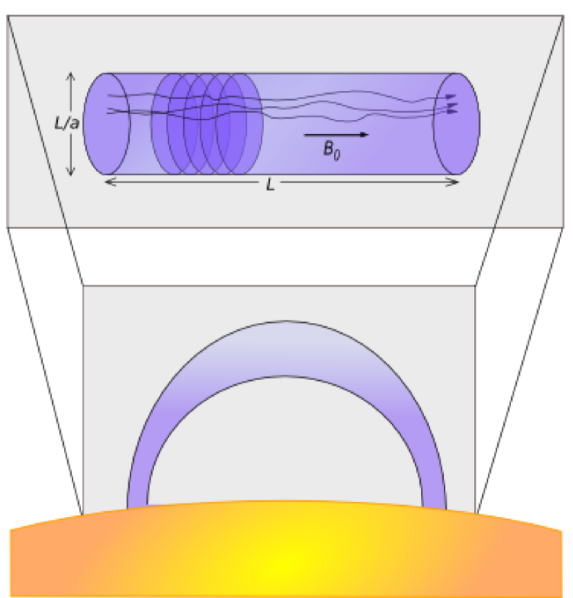
?figurename? 1: Layout of the Shell-Atm model in the case of a coronal loop: shell-models are piled up along $\@vec{B}_{\parallel}$ (top) and represent a loop, whose footpoints are anchored in the photosphere (bottom). Reproduced from Buchlin & Velli (2007).

The model gives the energy per unit volume as $E_{V}=\frac{1}{2}\rho\sum_{n}(|u_{n}|^{2}+|b_{n}|^{2})$ and the heating (power of energy dissipation) per unit volume is calculated by computing the time derivative of $E_{V}$. This gives $H_{V}=\rho\sum_{n}k_{n}^{2}(\nu|u_{n}|^{2}+\eta|b_{n}|^{2})$ (where all quantities may depend on $z$): the heating per unit length is $H_{L}=H_{V}\pi\ell^{2}/4$ and the heating per unit mass is $H_{M}=H_{V}/\rho$ (again, all quantities may depend on $z$).

2.2 The HydRad model

The HydRad code (Bradshaw & Mason 2003) is a hydrodynamic model of a coronal loop with a self-consistent treatment of radiation (including non-equilibrium ion populations). In this paper it is simply used in an equilibrium run, so as to get a hydrostatic profile $\rho_{\textsc{HydRad}}(z)$ of the mass density along the loop. We used an isothermal hydrostatic solution so that the density along the loop is stratified due to gravity alone. Since there is no thermal flux (isothermal temperature profile) the background heating and radiation are in balance, and are thus identically zero. Therefore, we make no assumptions about the nature of the background heating; once coupled to the Shell-Atm model, all of the energy released into the loop will be from the shell model only. The loop length used in this run was $10\>\mathrm{Mm}$.

2.3 A simple phenomenology for the energy and heating profiles

In this section we discuss what profiles of the fields, energy and dissipation power along the loop would be expected from a simple phenomenology.

A mass density profile $\rho(z)$, a magnetic field profile $B_{\parallel}(z)$ and a profile $\nu(z)$ of the dissipation coefficient (kinetic or magnetic) are given (in model units). The Elsässer fields $Z^{\pm}$ are assumed to be both of the same order of magnitude $Z$ (which is reasonable in a loop). The effects of energy dissipation and of non-linear interactions on the magnitudes of the fields are assumed to be negligible.

The conservation of energy fluxes $\phi_{E}^{\pm}=\pm b_{\parallel}E_{V}^{\pm}\pi\ell^{2}/4$ together with the conservation of the magnetic flux $\phi_{B}=B_{\parallel}\pi\ell^{2}/4$ gives then a profile $E_{V}\propto\rho^{1/2}$ of the energy per unit volume. The dissipation power per unit volume is $H_{V}=\rho\nu k_{\perp}^{2}Z^{2}\propto\nu k_{\perp}^{2}\rho^{1/2}$ for a fixed $k_{\perp}$. However, one must bear in mind that when a wave travels along the loop (with non-linear interactions neglected), the associated $k_{\perp}$ is affected by the variation of the width of the loop (in the model, the wave stays in the same shell $n$ of the model): $k_{\perp}=k_{n}(z)=k_{0}(z)\lambda^{n}$, with $k_{0}\propto B_{\parallel}^{1/2}$ because of the conservation of magnetic flux. For this reason, for a linear wave in the shell $n$, $H_{V}^{(n)}\propto\nu B_{\parallel}\rho^{1/2}$.

3 Numerical simulations

For all simulations, we choose model units so that the length of the loop is $L=1$, and so as to have the below-mentioned values for the magnetic field $B_{\parallel}^{f}$ and for the mass density $\rho_{f}$ at the footpoints. Conversion factors to physical units for a sample loop are given in Table 1, but to use the same simulations for other loops with different physical parameters it is sufficient to take different values for the basic conversion factors $M$, $L$ and $T$ for mass, distance and time respectively. We stress that these conversion factors do not necessarily represent typical values of the actual physical quantities in the loop (the model variables are not necessarily of the order of unity in model units; this will especially be true for the diffusion coefficients).

If $\rho_{\textsc{HydRad}}(z)$ is the density profile from the equilibrium run of the HydRad code (see Sec. 2.2), we define $R(z)=\rho_{\textsc{HydRad}}(z)/\rho_{\textsc{HydRad}}(0)$, with $0$ being the position of one footpoint. $R$ varies between $R_{t}=1/30$ at the loop top and $R_{f}=1$ at the footpoints. The profiles of mass density and Alfvén speed are then chosen as a function of $R$ as specified in Table 2 for each of the runs. The physical conditions are chosen to be the same at the footpoints in each run ($\rho_{f}=1/R_{t}$ and $B_{\parallel}^{f}=1$), so that the boundary conditions of the model remain the same in the different runs.

A typical value for the diffusivity coefficients $\nu$ and $\eta$ is $5\,10^{-10}$ in model units (see Table 2 for the exact values used in each run), i.e. of the order of $5\,10^{3}\>\mathrm{m^{2}/s}$; typical Reynolds and magnetic Reynolds numbers are $10^{6}$. This is lower than in the real corona (diffusivity coefficients are higher than in the real corona) but it represents a huge improvement over direct numerical simulations of MHD.

?tablename? 1: Conversion factors between model units and S.I. physical units: expression in the general case and value for a typical modelled loop.

	Conversion factor to S.I. physical units
Quantity	Expression	Typical value
Mass	$M$	$10^{9}\>\mathrm{kg}$
Length, distance	$L$	$10^{7}\>\mathrm{m}$
Time	$T$	$10\>\mathrm{s}$
Velocity, Alfvén speed	$LT^{-1}$	$10^{6}\>\mathrm{m\,s^{-1}}$
Magnetic field	$\sqrt{\mu_{0}}M^{1/2}L^{-1/2}T^{-1}$	$1.1\,10^{-3}\>\mathrm{T}$
Mass density	$ML^{-3}$	$10^{-12}\>\mathrm{kg\,m^{-3}}$
Diffusivity	$L^{2}T^{-1}$	$10^{13}\>\mathrm{m^{2}\,s^{-1}}$
Energy per unit volume	$ML^{-1}T^{-2}$	$1\>\mathrm{J\,m^{-3}}$
Power per unit volume	$ML^{-1}T^{-3}$	$10^{-1}\>\mathrm{W\,m^{-3}}$

We use the model with $1000$ planes piled up along $\@vec{B}_{\parallel}$, and each of these has $18$ shells ($n=0,\ldots 17$). Each of the simulations is run during $500$ units of time (after an initial phase of energy growth), which corresponds to the order of 100 large-eddy turn-over times. Profiles of the energy and of the dissipation per unit volume are averaged over the duration of the runs.

?tablename? 2: Summary of the parameters of the modelled loop for different runs, in model units.

Run	$\rho R_{t}$	$b_{\parallel}/R_{t}^{1/2}$	$B_{\parallel}$	$\nu/10^{-10}$	$\eta/10^{-10}$
(u)	$1$	$1$	$1$	$5$	$5$
(a)	$R$	$R^{-1/2}$	$1$	$5$	$5$
(b)	$R^{1/2}$	$R^{-1/4}$	$1$	$5$	$5$
(c)	$R^{1/4}$	$R^{-1/8}$	$1$	$5$	$5$
(A)	$R$	$R^{-1/4}$	$R^{1/4}$	$5$	$5$
(B)	$R^{1/2}$	$R^{-1/8}$	$R^{1/8}$	$5$	$5$
(C)	$R^{1/4}$	$R^{-1/16}$	$R^{1/16}$	$5$	$5$
(p)	$R$	$R^{-1/2}$	$1$	$0.5(R/R_{t})^{-7/2}$	$0.5(R/R_{t})^{3/2}$
(q)	$R$	$R^{-1/2}$	$1$	$50(R/R_{t})^{-7/2}$	$0.5(R/R_{t})^{3/2}$
(r)	$R$	$R^{-1/2}$	$1$	$10^{2}(R/R_{t})^{-7/2}$	$10^{-2}(R/R_{t})^{3/2}$
(s)	$R$	$R^{-1/2}$	$1$	$10^{2}(R/R_{t})^{-7/2}$	$10^{-4}(R/R_{t})^{3/2}$
(t)	$R$	$R^{-1/2}$	$1$	$10^{2}(R/R_{t})^{-7/2}$	$10^{-6}(R/R_{t})^{3/2}$

3.1 Test case: uniform loop

We present run (u) as a test case, where the mass density, magnetic field, Alfvén speed and diffusion coefficients are all uniform (as in Buchlin & Velli 2007). Figure 2 shows that the time-average profile of the total energy per unit volume is uniform along the loop, with the magnetic energy dominating. The kinetic energy density is also uniform except near the footpoints, where it gets lower because of the boundary conditions ($u_{f}\ll\@vec{B}_{\parallel}$).

The energy dissipation (right panel of Fig. 2) is slightly non-uniform: although the phenomenology of Sec. 2.3 suggests a uniform profile, there is a drop near the footpoints and an enhancement near the loop top; the former can be attributed mainly to the contribution of the profile of kinetic energy dissipation, and the latter to the profile of the magnetic energy dissipation. The ratio of total dissipation power in the central $10\%$ of the loop length to the total dissipation power in both $5\%$ of the loop length at the footpoints is $1.5$.

A second observation is that the ratio of magnetic to kinetic energy dissipation is lower than the ratio of the magnetic to kinetic energy. This is because most magnetic energy is concentrated at large scales as can be seen on the spectra of Fig. 3, which do not dissipate as much as the smaller scales. Then the relative weight of the kinetic dissipation in the total dissipation is increased compared to the weight of the kinetic energy in the total energy; as the kinetic dissipation profile is lower at the footpoints (because of the boundary condition with $u_{f}\ll\@vec{B}_{\parallel}$), this explains the non-uniform shape of the total dissipation profile. This kind of effect needs to be kept in mind when analyzing the other runs.

?figurename? 2: Average profiles of the energy (left) and dissipation power (right) per unit volume, as a function of the position $z$ along the loop, for run (u). The dotted lines are the kinetic energy or dissipation power, the dashed line the magnetic energy or dissipation power, and the plain line is the total.

?figurename? 3: Time-averaged kinetic (dots) and magnetic (dashes) perpendicular 1D energy spectra in the loop for run (u). A line of slope $-5/3$ is shown for reference. These spectra are representative of the spectra obtained for the other runs, although there can be some variations between runs.

3.2 Loop with a non-uniform mass density

We now consider a more realistic loop, with a non-uniform mass density determined by the HydRad model. The ability to take into account a non-uniform mass density (as well as a variable axial magnetic field: see later) is an important advantage of the Shell-Atm model when compared to the model of Nigro et al. (2004) as used by Reale et al. (2005). Run (a) is performed using a mass density profile $\rho(z)=R(z)/R_{t}$ (Fig. 4). In runs (b) and (c) we use $R^{1/2}/R_{t}$ and $R^{1/4}/R_{t}$ for the mass density profiles, so as to assess the effect of smoother profiles.

Loops seen with Yohkoh and TRACE have only a slight width enhancement at the top relative to the footpoints (Klimchuk et al. 1992; Klimchuk 2000; Watko & Klimchuk 2000). It is thus reasonable to assume a uniform axial magnetic field along such loop. In the model we set $B_{\parallel}={b_{\parallel}}^{t}\sqrt{\rho_{t}}$ with ${b_{\parallel}}^{t}=1$ ($\mu_{0}=1$ in model units). The Alfvén speed is then $b_{\parallel}(z)={b_{\parallel}}^{t}(\rho(z)/\rho_{t})^{1/2}$, a function of $z$, as shown in Fig. 4. Consequently the waves are partially reflected due to the Alfvén speed gradient .

The resulting time-averaged profiles of the energy per unit volume $E_{V}(z)$ and of the heating per unit volume $H_{V}(z)$ are shown in Fig. 5. The striking result is that in all these cases, including run (a) which has steep gradients of density and Alfvén speed, the effect of the non-uniform density on the heating profiles is very limited. For run (a) for example, while the phenomenology of Sec. 2.3 predicts a dependence in $\rho^{1/2}$ for both energy density and dissipation, i.e. a ratio $\approx 5.5$ between the footpoints and the loop top, the actual ratio is only about $1.3$ between the highest values (near the footpoints) and the lowest values, for both energy and and dissipation. For runs (b) and (c) (which have shallower density gradients), the profiles are even closer to being uniform.

We performed fits of each of these profiles to a power-law $\rho^{\alpha}$ of the mass density (Table 3). The domain for the fit was restricted to the central $90\%$ of the loop, to avoid effects due to the boundary conditions. In cases (a) and (b), the fit of the heating profile gives an index $\alpha_{H}$ close to $0$ for the power-law $\rho^{\alpha_{H}}$ (taking into account the error bars of the fit; see Table 3 for the detailed results of the fits). Each of the individual profiles cannot be considered as uniform (as would be the case if the fit was perfect and with $\alpha_{H}=0$), but they are still considerably more uniform than that expected from the steep gradient of the mass density $\rho$.

The fit of the energy profiles gives an index $7.1\,10^{-2}<\alpha_{E}<9.4\,10^{-2}$ (in all three cases, taking into account the error bars). The profile of energy is thus also much more uniform than expected from the phenomenology ($\alpha=1/2$). This is surprising as it means that, when going from the footpoints to the loop top, the energy decreases slower than what would be expected from the conservation of the energy flux (under the assumptions detailed in Sec. 2.3). The discrepancies between the phenomenology and the results are discussed further in Sec. 4.

?figurename? 4: Profiles of mass density $\rho$, Alfvén speed $b_{\parallel}$ and gradient of Alfvén speed $\,\mathrm{d}b_{\parallel}/\,\mathrm{d}z$ for run (a), as a function of the position $z$ along the loop.

?figurename? 5: Average profiles of the energy (left) and dissipation power (right) per unit volume, as a function of the position $z$ along the loop, for runs (a), (b) and (c) (from top to bottom). The dotted lines are the kinetic energy or dissipation power, the dashed line the magnetic energy or dissipation power, and the plain line is the total (same as in Fig. 2).

?tablename? 3: Summary of the indices $\alpha_{E}$ and $\alpha_{H}$ for the power-law fits $E_{V}\propto\rho^{\alpha_{E}}$ and $H_{V}\propto\rho^{\alpha_{H}}$, (1) expected from the phenomenology of Sec. 2.3 and (2) obtained from the numerical simulations, for the runs with uniform dissipation coefficients. The fits from the simulations are performed on time-averaged profiles and on the central $90\%$ of the loop.

Run	$\alpha_{E}$ (1)	$\alpha_{E}$ (2)	$\alpha_{H}$ (1)	$\alpha_{H}$ (2)
(a)	$1/2$	$(8.50\pm 0.05)10^{-2}$	$1/2$	$(7.39\pm 0.09)10^{-2}$
(b)	”	$(7.14\pm 0.02)10^{-2}$	”	$(-8.98\pm 0.15)10^{-2}$
(c)	”	$(9.42\pm 0.01)10^{-2}$	”	$(-2.85\pm 0.03)10^{-1}$
(A)	”	$(3.15\pm 0.00)10^{-1}$	$3/4$	$(4.59\pm 0.01)10^{-1}$
(B)	”	$(3.18\pm 0.00)10^{-1}$	”	$(3.81\pm 0.01)10^{-1}$
(C)	”	$(3.05\pm 0.00)10^{-1}$	”	$(1.96\pm 0.04)10^{-1}$

Although the comparison of the heating in loops of different lengths is out of the scope of this paper, we have also performed a simulation of a $40\>\mathrm{Mm}$-long loop. In this case a uniform chromospheric temperature yields unrealistically low coronal densities, so the loop has been divided into a $20\,000\>\mathrm{K}$ chromosphere and, from the points where the density has been divided by $100$ compared to the footpoints, a $1\>\mathrm{MK}$ corona. Although the ratio of footpoint to loop top densities is higher than in the other simulations presented in this paper, the average heating profile remains quasi-uniform ($\alpha_{H}=(3.13\pm 0.66)10^{-2}$). Therefore, when the heating model Shell-Atm is considered alone in a hydrostatic loop (i.e. neglecting the feedback effects of the cooling processes), longer loops do not seem to behave differently than shorter loops.

3.3 Loop with non-uniform mass density and magnetic field

In very large structures like coronal streamers, it is likely that the magnetic field gets weaker with altitude. We model this variation through a dependence on the mass density: the axial magnetic field of the loop is chosen to be $B_{\parallel}(z)=b_{\parallel}\sqrt{\mu_{0}\rho(z)}(\rho(z)/\rho_{t})^{-1/4}$ (the exponent $1/4$ has been chosen so as to minimize both the gradients of magnetic field and of Alfvén speed for a given density profile). The Alfvén speed is then $b_{\parallel}(\rho(z)/\rho_{t})^{1/4}$.

Runs (A), (B) and (C) are performed with this magnetic field profile, and the same density profiles as runs (a), (b) and (c) respectively (see Table 2). For run (A) for example, the ratio of the magnetic field between the footpoints and the loop top is then $2.3$.

?figurename? 6: Average profiles of the energy (left) and dissipation power (right) per unit volume, as a function of the position $z$ along the loop, for runs (A), (B) and (C) (from top to bottom). The dotted lines are the kinetic energy or dissipation power, the dashed line the magnetic energy or dissipation power, and the plain line is the total (same as in Fig. 2).

The resulting time-averaged profiles of the energy and the heating per unit volume are shown in Fig. 6. In all cases (and especially (A), which has the steepest density and magnetic field gradients) the heating is enhanced at the footpoints. The results of the power-law fits of the heating profiles as a function of the mass density are also shown in Table 3; we get $0.19<\alpha_{H}<0.46$ in all three cases (taking into account the error bars) whereas the phenomenology of Sec. 2.3 predicts $\alpha_{H}=3/4$.

This enhancement of the dissipation power at the footpoints can be seen as a consequence of the higher energy per unit volume there. Indeed, the power-law fits of the energy profiles give $0.30<\alpha_{E}<0.32$ in all three cases, as seen in Table 3 (taking into account the error bars), whereas the phenomenology predicts $\alpha_{E}=1/2$. Again, there is more energy at the loop top than what would be expected from the conservation of the energy flux.

3.4 Loop with non-uniform mass density and diffusivity coefficients

Up to now the diffusion coefficients have been assumed to be uniform, but this is not the case if the temperature profile is not uniform. So as to take this effect into account, we consider a different situation than in the previous sections, with the same density profile $\rho(z)=R(z)/R_{t}$ as runs (a) and (A), but assuming now that the loop has a uniform pressure and that the law of perfect gases holds, hence a variation of a factor $R_{f}/R_{t}=30$ of the temperature between the footpoints and the loop top. With these assumptions, the variations of the diffusivity coefficients in the magnetized plasma as obtained from Braginskii (1965) are in $T^{7/2}$ for the kinematic viscosity and in $T^{-3/2}$ for the magnetic diffusivity, where $T$ is the plasma temperature (which is only known in our model from the density $\rho$ and the assumptions we make in this section). We thus choose profiles $\nu=\nu_{t}R^{-7/2}$ and $\eta=\eta_{t}R^{3/2}$ for the kinematic viscosity and for the magnetic diffusivity respectively, where $\nu_{t}$ and $\eta_{t}$ are the values of $\nu$ and $\eta$ that we have chosen at the loop top.

We perform runs (p), (q), (r), (s) and (t) at different magnetic Prandtl numbers at loop top: $Pr_{M}^{t}=\nu_{t}/\eta_{t}=1$, $10^{2}$, $10^{4}$, $10^{6}$ and $10^{8}$ respectively (see Table 2). With the profiles we use, the magnetic Prandtl number is $(R_{f}/R_{t})^{5}$ times lower at the footpoints than at the loop top, i.e. $2.4\,10^{7}$ times lower: it is $Pr_{M}^{f}=4\,10^{-8}$, $4\,10^{-6}$, $4\,10^{-4}$, $4\,10^{-2}$ and $4$ for runs (p), (q), (r), (s) and (t) respectively (see Fig. 7). These ranges of magnetic Prandtl numbers and of diffusivity coefficients, which are impossible to explore with direct numerical simulations, are easily managed by the Shell-Atm model.

?figurename? 7: Profiles of the dissipation coefficients $\nu$ (kinematic viscosity; dots) and $\eta$ (magnetic diffusivity; dashs) used in runs (p), (q), (r), (s) and (t) (from left to right and top to bottom).

?figurename? 8: Average profiles of the energy (left) and dissipation power (right) per unit volume, as a function of the position $z$ along the loop, for runs (p), (q), (r), (s) and (t) (from top to bottom). The dotted lines are the kinetic energy or dissipation power, the dashed line the magnetic energy or dissipation power, and the plain line is the total (same as in Fig. 2).

Compared to run (a), which has otherwise the same parameters, the profiles of the kinetic and magnetic energies, seen in Fig. 8, are barely affected: such small dissipation coefficients, which allow for a wide turbulent inertial range to develop, have almost no influence on the energy content as a function of the position along the loop, and the energy does not decrease significantly with altitude as a result of the dissipation.

However, as expected, the profiles of both the kinematic viscosity $\nu$ and the magnetic diffusivity $\eta$ have an effect on the kinetic ($H_{V}^{u}$) and magnetic ($H_{V}^{b}$) dissipation powers (right panels of Fig. 8): the profile of $H_{V}^{u}$ is mainly affected by the profile of $\nu$ and the profile of $H_{V}^{b}$ is mainly affected by the profile of $\eta$. The combination of both gives a heating profile which is enhanced either at the footpoints (runs (p) and (q)), at the loop top (runs (s) and (t)) or both (run (r)). Heating enhancements at the footpoints are mainly due to magnetic energy dissipation, while a heating enhancement at the loop top is mainly due to kinetic energy dissipation. Note also that, as the kinetic energy is smaller in all cases than the magnetic energy, the ratio of the kinetic over magnetic dissipation is lower than what would be expected from the mere ratio of the kinematic viscosity over the magnetic diffusivity.

The fits of the kinetic (resp. magnetic) dissipation profiles to a power-law $\rho^{\alpha}$ are in most cases broadly consistent with the expected value $\alpha=-7/2$ (resp. $3/2$), although there are important differences between the different runs. The ratios between the kinetic (resp. magnetic) dissipation power near the footpoints and at the loop top are also broadly consistent with the same ratio for $\nu$ (resp. $\eta$). Given the parameters of the model, this ratio can become very large but it is again easily managed by the Shell-Atm model.

4 Discussion

We have presented a set of simulations of a coronal magnetic loop containing a highly turbulent MHD plasma, with Reynolds numbers up to $10^{6}$, a variation between the loop top and the footpoints by a factor of up to $30$ for the density and up to the order of $10^{7}$ for the magnetic Prandtl number. These ranges of physical parameters cannot be reached by direct numerical simulations.

The spatial distributions of the energy and of the heating as a function of the position along the loop have been obtained. The profiles of energy do not have a strong dependence on the position along the loop (runs (a) to (c)), except when the flux tube is expanding (runs (A) to (C)): in this case the energy per unit volume is higher near the footpoints, where the magnetic field is higher. The profiles of the heating (the dissipation of energy per unit volume) also have a low dependence on position when only the density varies. If the flux tube is expanding, the behavior of the heating profile is quite similar to that of the energy profile: the heating is higher near the footpoints.

When we look at runs (a) to (C) the profiles of energy and heating are shallower than what is expected from the simple linear phenomenology introduced in Sec. 2.3. We now try to explain the origin of these discrepancies. First, one might expect that the dissipation occurring during the wave propagation to the loop top would make the profile of energy $E_{V}$ deeper instead of shallower; however, the comparison of the energy profiles in runs (p) to (t) (Fig. 8 left) with run (a) shows that this effect remains unnoticeable. The origin of the energy profile is still unclear.

Assuming now an energy profile $E_{V}\propto\rho^{\alpha_{E}}$ (with $\alpha_{E}$ coming from the fits of the results of the different runs), the dissipation profile in a given shell $n$ is $H_{V}^{(n)}\propto B_{\parallel}\rho^{\alpha_{E}}$, i.e. $\alpha_{H}\approx 0.1$ for runs (a) to (c) and $\alpha_{H}\approx 0.55$ for runs (A) to (C). This is already closer to the simulations results (Table 3) than the purely phenomenological predictions of $1/2$ and $3/4$ respectively. The remainder of the difference could be explained by the effect observed in run (u): the ratio of the kinetic dissipation profile (which is low at footpoints due to the velocity boundary condition at the photosphere) over the magnetic dissipation profile is increased compared to the ratio of the kinetic energy profile over the magnetic energy profile because of the concentration of magnetic energy at the larger scales in the loop. Thus the slow motions of the loops footpoints anchored in the photosphere and the build-up of magnetic energy mainly at large scales have a decisive influence on the determination of the profiles of heating in coronal loops.

Another, more subtle, effect is related to the profiles of the nonlinear and dissipation timescales. For a given $k_{\perp}$, the non-linear time scale is $\tau_{\textrm{NL}}=1/k_{\perp}Z$ and the dissipation time scale is $\tau_{\nu}=1/\nu k_{\perp}^{2}$. Taking into account the energy profile and the variation of $k_{\perp}$ for a given shell $n$ (like in Sec. 2.3), the non-linear time scale is $\tau_{\textrm{NL}}^{(n)}\propto\rho^{(1-\alpha_{E})/2}/B_{\parallel}^{1/2}$ and the dissipation time scale is $\tau_{\nu}^{(n)}\propto 1/\nu B_{\parallel}$ for a given shell $n$. This means that for runs (a) to (c), the dissipation time scale does not depend on position while the nonlinear timescale ($\approx\rho^{0.45}$) is shorter at the loop top: the transfer of energy to the small scales is more efficient, and as a consequence, the dissipation power is higher at the loop top than what is expected from the phenomenology of Sec. 2.3. This is in accordance to what is seen in the simulation results (a shallower profile of dissipation). For runs (A) to (C) the nonlinear ($\propto\rho^{0.23}$) and dissipation ($\propto\rho^{-1/4}$) timescales vary in opposite directions: the nonlinear terms are more efficient at the loop top, but they need to bring the energy further in the spectrum. However, the different $k_{\perp}$-dependence of both competing timescales means that the enhanced efficiency of the nonlinear transfer “wins” over the displacement of the dissipation scale: again, as seen in the simulations, the heating profile is shallower than expected before.

Runs (p) to (t) point out the additional role of the variation of the diffusion coefficients as a function of temperature (and thus as a function of position along the loop), which seems to have been overlooked in previous works. The profile of the kinetic (magnetic) energy dissipation follows approximately the profile of the kinetic (magnetic) diffusion coefficient respectively. The diffusion coefficients have thus a direct influence on the energy dissipation, and as they strongly vary with temperature, this yields a strong variation of the dissipation power along the loop. Furthermore, as both diffusion coefficients vary in opposite ways with temperature, the heating can be enhanced at the footpoints, at the loop top or both, depending on the magnetic Prandtl numbers in the loop.

Although these results seem to be straight forward, this had never been modelled in the context of solar coronal heating, as the precise values of $\nu$ and $\eta$ are usually considered unimportant to get averages of the heating: the main argument for that is that energy is dissipated at the end of the inertial range, at whichever scale (or wavenumber) this end is (Galsgaard & Nordlund 1996). However, these values actually have an importance because (1) they discriminate between low- and high-Reynolds-number physics, with effects like intermittency appearing only at very high Reynolds numbers; (2) when waves propagate between regions with different diffusion coefficients, we have shown in this paper that the profiles of these coefficients contribute to the determination of the profile of the heating.

These simple simulations shed light on the consequences on heating profiles of the complex interactions between some of the physical effects that come into play in a non-uniform turbulent coronal loop: conservation of energy and magnetic fluxes, accumulation of large-scale magnetic field in a loop submitted to photospheric motions, nonlinear effects, and non-uniformity of the viscosity and magnetic diffusivity coefficients. However, many processes have not been included in these simulations, such as heat transport (conduction and radiation), flows, gravity, MHD processes overlooked by the shell-models, and kinetic effects. Future developments may include the heat transport and the subsequent computation of emitted radiation, especially in UV. In addition to completing the picture of the nanoflare-like processes involved in heating and cooling of loops, this will allow the comparison of such models to data from new instruments (such as Hinode/EIS) that observe the plasma at higher temperatures than previous instruments, at earlier stages of heating events.