Scaling Relations and Mass Calibration of the X-ray Luminous Galaxy Clusters at redshift $\sim 0.2$: XMM-Newton Observations

We present the X-ray properties and scaling relations of a flux-limited morphology-unbiased sample of 12 X-ray luminous galaxy clusters at redshift around 0.2 based on XMM-Newton observations. The scaled radial profiles are characterized by a self-similar behavior at radii outside the cluster cores ($>0.2r_{500}$) for the temperature ($T\propto r^{-0.36}$), surface brightness, entropy ($S\propto r^{1.01}$), gas mass and total mass. The cluster cores contribute up to 70% of the bolometric X-ray luminosity. The X-ray scaling relations and their scatter are sensitive to the presence of the cool cores. Using the X-ray luminosity corrected for the cluster central region and the temperature measured excluding the cluster central region, the normalization agrees to better than 10% for the cool core clusters and non-cool core clusters, irrelevant to the cluster morphology. No evolution of the X-ray scaling relations was observed comparing this sample to the nearby and more distant samples. With the current observations, the cluster temperature and luminosity can be used as reliable mass indicators with the mass scatter within 20%. Mass discrepancies remain between X-ray and lensing and lead to larger scatter in the scaling relations using the lensing masses (e.g. $\sim 40$% for the luminosity–mass relation) than using the X-ray masses ($<20$%) due to the possible reasons discussed.

osmology: observations – Galaxies: clusters: general – X-rays: galaxies: clusters – (Cosmology:) dark matter

1 Introduction

Both the gravitational growth of density fluctuations and the expansion history of the Universe can be used to constrain the cosmology.

The gravitational growth of the fluctuation can be measured by, e.g. the evolution of the galaxy cluster mass function (e.g. Schuecker et al. 2003). The most massive clusters show the cleanest results in comparing theory with observations. The mass function of luminous galaxy clusters probes the cosmic evolution of large-scale structure (LSS) and is thus an extremely effective test of cosmological models. It is sensitive to the matter density, $\Omega_{\rm m}$, and the amplitude of the cosmic power spectrum on cluster scales, $\sigma_{8}$ (e.g. Schuecker et al. 2003).

The expansion history of the Universe can be used to determine the metric and thus to constrain the cosmological parameters. Typical examples are Supernova Ia (SN Ia, e.g. Astier et al. 2006) and galaxy clusters combining the Sunyaev-Zeldovich effect (Sunyaev & Zeldovich 1972, the SZ effect) and thermal Bremsstrahlung X-ray approaches (Molnar et al. 2002), in which the luminosity distance and volume are used to determine the metric, respectively.

The multi-pole structure of the cosmic microwave background (CMB) anisotropy power spectrum depends on the normalized overall amount of dark matter (DM) in the Universe. The WMAP three year results imply values of the parameters $\Omega_{\rm m}h^{2}$, $\Omega_{\rm b}h^{2}$, $h$, $n_{\rm s}$, and $\sigma_{8}$ of $0.127^{+0.007}_{-0.013}$, $0.0223^{+0.0007}_{-0.0009}$, $0.73^{+0.03}_{-0.03}$, $0.951^{+0.015}_{-0.019}$, and $0.74^{+0.05}_{-0.06}$ (Spergel et al. 2006). Combining the CMB approach with the other cosmological tests, e.g. galaxy cluster surveys, the large-scale galaxy distribution and/or SN Ia, is sensitive to the effects of dark energy, the density of which is characterized by the parameter $\Omega_{\Lambda}$ and its time evolution by the equation of state parameter $w(z)$ (e.g. Vikhlinin et al. 2002; Allen et al. 2004; Chen & Ratra 2004; Hu et al. 2006).

The construction of the mass function of galaxy clusters for large cosmological cluster samples is based on the cluster X-ray temperature/luminosity estimates and the mass–observable scaling relations (Reiprich & Böhringer 2002). A better understanding of the mass–observable scaling relations and their scatter is of prime importance for galaxy clusters as a unique means to study the LSS and thus to constrain the cosmological parameters (Voit 2005). Precise mass estimates and mass–observable scaling relations can potentially push the current measurement uncertainty (10–30%) of the cosmological tests to higher precision (Smith et al. 2003, 2005; Bardeau et al. 2006).

The mass distributions in galaxy clusters can be probed in a variety of ways using: (i) the X-ray gas density and temperature distributions under the assumptions of hydrostatic equilibrium and spherical symmetry, (ii) the velocity dispersion and spatial distribution of cluster galaxies, (iii) the distortion of background galaxies caused by the gravitational lensing effect, and (iv) the SZ effect. For the relaxed low-redshift clusters, the uncertainties are small in the masses measured from the precise intra-cluster medium (ICM) temperature and density profiles up to large radii (e.g. $r_{500}$) using X-ray observations of XMM-Newton and Chandra (Allen et al. 2004; Pointecouteau et al. 2005; Arnaud et al. 2005; Vikhlinin et al. 2006a). Particularly, the X-ray results for the relaxed clusters have achieved a very high level of precision ($<10$%) in Arnaud et al. (2005) and Vikhlinin et al. (2006a). The methods to measure cluster mass using the velocity dispersion of cluster galaxies and gravitational lensing are improving (Girardi et al. 1998; Smith et al. 2003, 2005; Bardeau et al. 2006). Up to now, it is technically more difficult for the SZ effect to resolve radial temperature distributions in galaxy clusters to obtain precise cluster masses but the future holds promise (Zhang & Wu 2003).

Some interpretations of the cluster dynamics, such as spherical symmetry and hydrostatic equilibrium, are required to obtain the cluster masses for the X-ray approach (also for the SZ effect). Substructure is observed in galaxy clusters and the frequency of its occurrence in ROSAT observations has for example been estimated to be of the order of about $52\pm 7$% (Schuecker et al. 2001). Using high quality XMM-Newton data, Finoguenov et al. (2005) found that substructures (on $>10$% level) can be observed in all the clusters in the REFLEX-DXL sample at $z\sim 0.3$. Based on the strong lensing results using high resolution HST data, Smith et al. (2005) measured the substructure fractions and identified the clusters with multi-modal DM morphologies. The up-coming XMM-Newton/Chandra results of comprehensive samples without exclusion of the mergers (HIFLUGS, Reiprich & Böhringer 2002, Reiprich 2006; LP, Böhringer et al. 2007), would be promising to investigate the mass measurement accuracy and the scaling relations for a morphology-unbiased sample at low redshifts.

Independent of the X-ray method, gravitational lensing provides a direct measure of projected cluster masses irrespective to their dynamical state. Comparison of ground-based lensing data including estimated arc redshifts with ASCA/ROSAT X-ray data show that the masses between X-ray and lensing are closely consistent for relaxed clusters (Allen 1998). However, detailed investigation with high quality (HST/XMM-Newton/Chandra) data reveals that for a few apparently ”relaxed” clusters in X-rays there remain large mass discrepancies between X-ray and lensing, especially on small scales, e.g. CL0024$+$17 (Kneib et al. 2003; Ota et al. 2004; Zhang et al. 2005a) and Abell 2218 (Soucail et al. 2004; Smith et al. 2005; Pratt et al. 2005). Stanek et al. (2006) illustrate the interplay between parameters and sources of systematic error in cosmological applications using galaxy clusters and stress the need for independent calibration of the $L$–$M$ relation such as gravitational weak lensing and X-ray approaches. It is extremely important to investigate cluster dynamics and to calibrate the scaling relations of a set of morphology-unbiased cluster samples at different redshifts to improve the understanding of intrinsic scatter and to control the sources of systematic errors.

Recently two morphology-unbiased flux-limited samples at medium distant redshifts were constructed. One (Smith et al. 2005; Bardeau et al. 2005, 2006; hereafter the pilot LoCuSS sample) is in the redshift range $0.176<z<0.253$ with $L\leavevmode\nobreak\ \geq\leavevmode\nobreak\ 8.0\times 10^{44}\leavevmode\nobreak\ {\rm erg\leavevmode\nobreak\ s^{-1}}$ based on the XBACS in Ebeling et al. (1996). The other (Zhang et al. 2004a, 2006; Finoguenov 2005; Böhringer et al. 2006; the REFLEX-DXL sample) is in the redshift range $0.258<z<0.308$ with $L\leavevmode\nobreak\ \geq\leavevmode\nobreak\ 5.9\times 10^{44}\leavevmode\nobreak\ {\rm erg\leavevmode\nobreak\ s^{-1}}$ based on the REFLEX survey in Böhringer et al. (2004). The selection effect is well understood for both samples (Smith et al. 2005; Böhringer et al. 2006), consisting of massive galaxy clusters spanning the full range of cluster morphologies (Bardeau et al. 2006; Zhang et al. 2006). Using the same method described in Zhang et al. (2006) for the REFLEX-DXL sample, we present here the studies of the pilot LoCuSS sample of 12 clusters (Abell 2219 is flared) based on high quality XMM-Newton observation. Smith et al. (2005) performed the strong lensing studies for most clusters in this sample except for Abell 1689 (Broadhurst et al. 2005a; Halkola et al. 2006) and Abell 2667 (Covone et al. 2006). The strong lensing studies of Abell 2218 can also be found in Kneib et al. (1996, 2004). Weak lensing analysis using HST, CFH12k and Subaru can be found in Bardeau et al. (2005, 2006) and Broadhurst et al. (2005b, for Abell 1689). We note that Abell 773 has no weak lensing mass estimates because no CFH12k data were taken for this cluster. We will compare the X-ray masses with the lensing masses (e.g. Kneib et al. 1996, 2004; Smith et al. 2003, 2005; Bardeau et al. 2006) to discuss possible mass discrepancies.

The main goals of this work are: (1) to derive precise cluster mass and gas mass fraction, (2) to investigate the self-similarity of the scaled profiles of the X-ray properties, (3) to seek for proper definition of the global quantities for the X-ray scaling relations with the least scatter, (4) to study the evolution of the X-ray scaling relations combining the pilot LoCuSS sample with the nearby and more distant samples, and (5) to compare the X-ray and lensing masses and to understand the scatter in the luminosity–mass scaling relations using the lensing masses.

The data reduction is described in Sect. 2 and the X-ray properties of the ICM of the sample in Sect. 3. We investigate the self-similarity of the scaled profiles of the X-ray properties in Sect. 4 and the X-ray scaling relations in Sect. 5. In Sect. 6 we compare the X-ray and lensing masses, discuss the peculiarities in individual clusters, and address the possible explanation for the scatter in the relation between the lensing mass and X-ray luminosity. We our the conclusions in Sect. 7. Unless explicitly stated otherwise, we adopt a flat $\Lambda$CDM cosmology with the density parameter $\Omega_{\rm m}=0.3$ and the Hubble constant $H_{\rm 0}=70$ km s^-1 Mpc^-1. We adopt the solar abundance table of Anders & Grevesse (1989). Confidence intervals correspond to the 68% confidence level. We apply the Orthogonal Distance Regression method (ODRPACK 2.01, e.g. Boggs et al. 1987) taking into account measurement errors on both variables to determine the parameters and their error bars of the fitting throughout this paper. We use Monte Carlo simulations for the uncertainty propagation on all quantities of interest.

2 Data reduction

2.1 Data preparation

All 13 clusters of the pilot LoCuSS sample at $z\sim 0.2$ were observed by XMM-Newton. However, the XMM-Newton observations of Abell 2219 are seriously contaminated by soft proton flares and are therefore excluded in this work. In total, 12 galaxy clusters observed by XMM-Newton were uniformly analyzed using the same method as described in Zhang et al. (2006). We use the XMMSAS v6.5.0 software for the data reduction. In Table 6 (See the electronic edition of the Journal) we present a detailed XMM-Newton log of the observations for all clusters.

All observations were performed with medium or thin filter for three detectors. The MOS data were taken in Full Frame (FF) mode except for MOS1 of Abell 1835. The pn data were taken in Extended Full Frame (EFF) mode or FF mode. For pn, the fractions of the out-of-time (OOT) effect are 2.32% and 6.30% for the EFF mode and FF mode, respectively. An OOT event file is created and used to statistically remove the OOT effect.

Above 10 keV (12 keV), there is little X-ray emission from clusters detected with MOS (pn) due to the low telescope efficiency at these energies. The particle background therefore dominates. The light curve in the energy range 10–12 keV (12–14 keV) for MOS (pn), binned in 100 s intervals, is used to monitor the particle background and to excise periods of high particle flux. Since episodes of “soft proton flares” (De Luca & Molendi 2004) were detected in the soft band, the light curve of the 0.3–10 keV band, binned in 10 s intervals, is used to monitor and to excise the soft proton flares. A 10 s interval bin size is chosen for the soft band to ensure a similar good photon statistic as for the hard band. The average and variance of the count rate have been interactively determined for each light curve from the count rate histogram. Good time intervals (GTIs) are those intervals with count rates below the threshold, which is defined as 2-$\sigma$ above the quiet average. The GTIs of both the hard band and the soft band are used to screen the data. The background observations are screened by the GTIs of the background data, which are produced using exactly the same thresholds as for the corresponding target observations. Settings of $FLAG=0$ and $PATTERN<13$ ($PATTERN<5$) for MOS (pn) are used in the screening process.

An “edetect_chain” command was used to detect point-like sources. Point sources were subtracted before the further data reduction.

2.2 Background subtraction

The background consists of several components exhibiting different spectral and temporal characteristics (e.g. De Luca & Molendi 2001; Lumb et al. 2002; Read & Ponman 2003). The background components can approximately be divided into two groups (e.g. Zhang et al. 2004a). One contains the background components showing significant vignetting, e.g. the cosmic X-ray background (CXB). The other contains the components with very little or no vignetting, e.g. particle-induced background.

Suitable background observations guarantee similar background components showing vignetting as for the target in the same detector coordinates. We choose the blank sky accumulations in the Chandra Deep Field South (CDFS) as background. The background observations were processed in the same way as the cluster observations. The CDFS observations used the thin filter for all detectors and the FF/EFF mode for MOS/pn. The medium filter was used for some target observations. Using the medium filter the background is different from the background using the thin filter at energies below 0.7 keV. Therefore we performed all the analysis at energies above 0.7 keV, in which the difference of the background is negligible. One can subtract the background extracted in the same detector coordinates as for the target. The cluster emission covers the inner part of the field of view (FOV), $R\leq 8^{\prime}$, and leaves the outer region to exam the background. The difference between the background in the target and background observations is taken into account as a residual background in the background subtraction. We applied such a double-background subtraction method specially developed for the medium distant clusters in Zhang et al. (2006) for spectral imaging analysis. More details about this method can be found in Zhang et al. (2006). Note independently a similar type of double background subtraction was earlier described in Pratt et al. (2001) and formalised in Arnaud et al. (2002). Here we only briefly described our double-background subtraction method (Zhang et al. 2006) as follows.

2.2.1 Spectral analysis

The spectra are extracted using the annuli within the truncation radius (see $r_{\rm t}$ in Sect. 3.3 and Table 1) corresponding to a $S/N$ of 3 of the observational surface brightness profile. The width of each annulus is selected to achieve precise temperature estimates. In order to obtain temperature measurements with uncertainties of $\sim 15$%, we used the criterion of $\sim 2000$ net counts per bin in the 2–7 keV band.

For a given target spectrum ($S_{\rm a}$) extracted from the annulus region with an area of $A_{\rm a}$ in the target observations, the background spectrum $B_{\rm a}$ is extracted in the background observations in the same detector coordinates as for the target spectrum. Hereafter we call the count rate ratio of the target and background observations limited to 10–12 keV (12–14 keV) for MOS (pn) as $c_{\rm AB}$. The first-order background spectrum is $c_{\rm AB}B_{\rm a}$. Because the cluster emission covers radii smaller than $8^{\prime}$ as shown in Sect. 3.3 (also see the truncation radius $r_{\rm t}$ in Table 1), the second-order background spectrum can be prepared as follows. A spectrum ($S_{\rm o}$) is extracted from the outer region (e.g. $8^{\prime}<R<8.33^{\prime}$) with an area of $A_{\rm o}$ in the target observations and its background spectrum ($B_{\rm o}$) in the same detector coordinates but in the background observations. The second-order background spectrum is $\frac{A_{\rm a}}{A_{\rm o}}(S_{\rm o}-c_{\rm AB}B_{\rm o})$. Assuming that the second-order background spectrum consists of the vignetted components such as CXB, the cluster spectrum is then given by $S_{\rm a}-c_{\rm AB}B_{\rm a}-\frac{A_{\rm a}}{A_{\rm o}}(S_{\rm o}-c_{\rm AB}B_{\rm o})$. We applied the second-order background spectrum with and without vignetting correction in the spectral analysis, and found that the difference in temperature and metallicity measurements increases with radius only up to 3% and 17%, respectively. Therefore the influence on the spectral measurements due to possible non-vignetted components such as the particle-induced background in the second-order background is negligible.

We performed spectral fitting of the MOS and pn data simultaneously with the XSPEC v11.3.1 software. Both the response matrix file (rmf) and auxiliary response file (arf) are used to recover the correct spectral shape and normalization of the cluster emission component. The following are usually taken into account for the rmf and arf, (i) a pure redistribution matrix giving the probability that a photon of energy $E$, once detected, will be measured in data channel PI, (ii) the quantum efficiency (without any filter, which, in XMM-Newton calibration, is called closed filter position) of the CCD detector, (iii) filter transmission, and (iv) geometric factors such as bad pixel corrections and gap corrections (e.g. around 4% for MOS). The vignetting correction to effective area for off-axis observations can be accounted for in the event lists by a weight column created by “evigweight”. All spectra are extracted considering the vignetting correction by the weight column in the event list produced by “evigweight”. The on-axis rmf and arf are co-created to account for (i) to (iv). We fixed the redshift to the peak value of the cluster galaxy redshift histogram (e.g. Smith et al. 2005; Bardeau et al. 2006; Covone et al. 2006) and the Galactic absorption to the weighted value in Dickey & Lockman (1990). A combined model “wabs$*$mekal” is then used with the on-axis arf and rmf in XSPEC for the fitting.

2.2.2 Image analysis

The 0.7–2 keV band is used to derive the surface brightness profiles. This ensures an almost temperature-independent X-ray emission coefficient over the expected temperature range. The vignetting correction to effective area is accounted for by the weight column in the event lists created by “evigweight”. Geometric factors such as bad pixel corrections are accounted for in the exposure maps. The width of the radial bins is $2^{\prime\prime}$. An azimuthally averaged surface brightness profile of the CDFS is derived in the same detector coordinates as for the target. The count rate ratios of the target and CDFS in the 10–12 keV band and 12–14 keV band for MOS and pn, respectively, are used to scale the CDFS surface brightness. The residual background in each annulus of the surface brightness is the count rate in the 0.7–2 keV band of the area scaled residual spectrum obtained in the spectral analysis. Both the scaled CDFS surface brightness profile and the residual background are subtracted from the target surface brightness profile. The background subtracted and vignetting corrected surface brightness profiles for three detectors are added into a single profile, and re-binned to reach a significance level of at least 3-$\sigma$ in each annulus. The truncation radii $r_{\rm t}$ are listed in Table 1. For most clusters, the particle-induced background varies by less than 10% comparing the background observations to the target observations. Therefore the dispersion of the re-normalization of the background observations is typically 10%. We take into account a 10% uncertainty of the scaled CDFS background and residual background.

2.3 PSF and de-projection

In the imaging analysis, we correct the PSF effect by fitting the observational surface brightness profile with a surface brightness profile model convolved with the empirical PSF matrices (Ghizzardi 2001).

Using the XMM-Newton point-spread function (PSF) calibrations in Ghizzardi (2001) we estimated the redistribution fraction of the flux. We found 20% for bins with width about $0.5^{\prime}$ and less than 10% for bins with width greater than $1^{\prime}$ neglecting energy dependent effects. We thus require an annulus width greater than $0.5^{\prime}$ in the spectral analysis. For such distant massive clusters, the PSF effect is only important within $0.5^{\prime}$, which corresponds $\leq 0.1r_{\rm 500}$ and introduces an uncertainty to the final results of the temperature profiles. This has to be investigated using deeper exposures with better photon statistic. The PSF blurring can not be completely considered for the spectral analysis the same way as for the image analysis because of the limited photon statistic.

The projected temperature is the observed temperature from a particular annulus, containing in projection the foreground and background temperature measurements. Under the assumption of spherical symmetry, the gas temperature in each spherical shell is derived by de-projecting the projected spectra. In this procedure, the inner shells contribute no flux to the outer annuli. The projected spectrum in the outermost annulus is thus equal to the spectrum in the outermost shell. The projected spectrum in the neighboring inner annulus has contributions from all the spectra in the shell at the radius of this annulus and in the outer shells (e.g. Suto et al. 1998). We de-projected the spectra as described in Jia et al. (2004) and performed the spectral fitting of the de-projected spectra in XSPEC to measure the radial temperature and metallicity profiles.

3 X-ray properties

The primary parameters of all 13 galaxy clusters are given in Table 1.

3.1 Density contrast

To determine the global cluster parameters, one needs a fiducial outer radius that was defined as follows. The mean cluster density contrast is the average density with respect to the critical density,

$$\Delta(<r)=\frac{3M(<r)}{4\pi r^{3}\rho_{\rm c}(z)}\;.$$ (1)

The critical density at redshift $z$ is $\rho_{\rm c}(z)=\rho_{\rm c0}E^{2}(z)$, where $E^{2}(z)=\Omega_{\rm m}(1+z)^{3}+\Omega_{\Lambda}+(1-\Omega_{\rm m}-\Omega_{\Lambda})(1+z)^{2}$. $r_{\Delta}$ is the radius within which the density contrast is $\Delta$. $M_{\Delta}$ is the total mass within $r_{\Delta}$. For $\Delta=500$, $r_{500}$ is the radius within which the density contrast is 500 and $M_{500}$ is the total mass within $r_{500}$. For $\Delta=2500$, $r_{2500}$ is the radius within which the density contrast is 2500 and $M_{2500}$ is the total mass within $r_{2500}$.

3.2 Temperature profiles

Temperature profiles probe the thermodynamical history of galaxy clusters. XMM-Newton (also Chandra), in contrast to earlier telescopes, has a less energy-dependent, smaller PSF, more reliable to study cluster temperature profiles. We de-projected the spectra as described in Sect. 2.3 and performed the spectral fitting in XSPEC to obtain the radial measurements of the temperature and metallicity. In the left panels of Fig. 1 (Also see Figs. 19–23 in the electronic edition of the Journal for the whole sample) we show the radial temperature profiles. The temperature profiles are approximated by

$$T(r)=T_{3}\exp[-(r-T_{1})^{2}/T_{2}]+T_{6}(1+r^{2}/T_{4}^{2})^{-T_{5}}+T_{7}\;,$$ (2)

where $T_{i}$, $i=1,...,7$, are simply for parameterization without physical meaning.

A cool core cluster (CCC) often shows both a peaked surface brightness profile and a steep temperature drop towards the cluster center. The classical mass deposition rate is derived by the radiative cooling model linking to the X-ray luminosity and thus the surface brightness profile (e.g. Peres et al. 1998). Chen et al. (2007) defined CCCs by two criteria, (1) scaled mass deposition rate $\dot{M}/M_{500}>10^{-13}/$yr, and (2) mass deposition rate $\dot{M}>0.01M_{\odot}$/yr. They found that 60% of the HIFLUGS sample are CCCs. With high resolution Chandra observations Vikhlinin et al. (2006b) defined CCCs by the cuspness of the surface brightness profile ($\alpha=\frac{d\log\rho_{\rm g}}{d\log r}>0.5$ at $r=0.04R_{500}$), and found that 2/3 of the clusters at $z<0.5$ and 15% at $z>0.5$ are CCCs, respectively. At $z>0.5$, they found no pronounced CCCs with $\alpha>0.7$.

For Abell 383, Abell 1835, Abell 2390 and Abell 2667, the temperatures drop to the values less than 70% of the maximum temperatures towards the cluster center. There is no strict division between CCCs and non-CCCs. We empirically define the CCC as the cluster whose temperature drop is greater than 30% of the peak temperature towards the cluster center. Hereafter these 4 clusters are called CCCs in the sample. As we show later, the 4 CCCs show shorter central cooling time, larger cooling radii (scaled to $r_{500}$) and lower central entropies compared to the non-CCCs. Using our definition of the CCC, the fractions of the CCCs are 33% and 15%, respectively, for the samples at $z\sim 0.2$ in this work and $z\sim 0.3$ in Zhang et al. (2006). This could indicate the evolution of the cool cores for massive clusters between $z\sim 0.2$ and $z\sim 0.3$ that the CCC fraction decreases with increasing redshift. This evolution could have already become important at $z\sim 0.3$.

However, the Poisson noise is quite significant for such small samples. Using re-randomization of the Monte Carlo simulated temperature profiles, the CCC fraction is 25–40% for the pilot LoCuSS sample, and 15–30% for the REFLEX-DXL sample, respectively. The difference in the fraction of the CCCs is actually not significant between the samples at redshift $\sim 0.2$ and 0.3. The evolution of the cool cores is thus not justified by the low significance of our result. Furthermore, the bootstrap effect accounting for missing clusters due to (1) the selection effect of the sample, and (2) the flares the XMM-Newton observational run, can only be recovered by mock catalogs in simulations. Additionally, the detection of the temperature drop in the cluster center becomes difficult for distant clusters, which can enhance the phenomenon that the CCC fraction decreases with the increasing redshift. A less resolution-dependent way to investigate the evolution of the cool cores is to use the luminosity based on the flux images, which will be addressed in Sect. 5.1.

3.3 Surface brightness

A $\beta$ model (e.g. Cavaliere & Fusco-Femiano 1976; Jones & Forman 1984) is often used to describe electron density profiles in clusters. To obtain an acceptable fit for all clusters in this sample, we adopt a double-$\beta$ model of the electron number density profile, $n_{\rm e}(r)=n_{\rm e01}(1+r^{2}/r_{\rm c1}^{2})^{-3\beta/2}+n_{\rm e02}(1+r^{2}/r_{\rm c2}^{2})^{-3\beta/2}$, where $n_{\rm e0}=n_{\rm e01}+n_{\rm e02}$ is the central electron number density (see Table 2), $\beta$ the slope parameter, and $r_{\rm c1}$ and $r_{\rm c2}$ the core radii of the inner and outer components, respectively (e.g. Bonamente et al. 2006). The soft band (e.g. 0.7–2 keV) X-ray surface brightness profile model $S(R)$, in which $R$ is the projected radius, is linked to the radial profile of the ICM electron number density $n_{\rm e}(r)$ as an integral performed along the line-of-sight for hot clusters ($T>2$ keV),

$$S_{\rm X}(R)\propto\int_{R}^{\infty}n_{\rm e}^{2}d\ell.$$ (3)

We fitted the observed surface brightness profile by this integral convolved with the PSF matrices (middle panels in Fig. 1, also see Figs. 19–23 in the electronic edition of the Journal for the whole sample) and obtained the parameters of the double-$\beta$ model of the electron density profile. The fit was performed within the truncation radius ($r_{\rm t}$, see Table 1) corresponding to a $S/N$ of 3 of the observational surface brightness profile. The truncation radii $r_{\rm t}$ are above $r_{500}$ for all 12 clusters. The cluster cores, referring to the central $\beta$ model of the double-$\beta$ model, span a broad range up to 0.2 $r_{500}$. The cluster cores for the CCCs are resolved with the current observations.

3.4 Mass distribution

We assume that the ICM is in hydrostatic equilibrium within the gravitational potential dominated by DM and its distribution appears spherical symmetry. The ICM can then be used to trace the cluster potential. The cluster mass is calculated from the X-ray measured ICM density and temperature distributions,

$$\frac{1}{\mu m_{\rm p}n_{\rm e}(r)}\frac{d[n_{\rm e}(r)T(r)]}{dr}=-\frac{GM(<r)}{r^{2}}\leavevmode\nobreak\ ,$$ (4)

where $\mu=0.62$ is the mean molecular weight per hydrogen atom. Following the method in Zhang et al. (2006), we use a set of input parameters of the approximation functions, in which $\beta$, $n_{\rm e0i}$, $r_{\rm ci}$ ($i=1,2$) represent the electron number density profile $n_{\rm e}(r)$ and $T_{\rm i}$ ($i=1,...,7$) represent the temperature profile $T(r)$, respectively, to compute the mean cluster mass. The mass uncertainties are propagated using the uncertainties of the electron number density and temperature measurements by Monte Carlo simulations as follows. For each cluster, we simulated electron density and temperature profiles of a sample of 100 clusters using the observed electron density and temperature profiles and their errors. The mass profiles and other properties of the 100 simulated clusters were calculated to derive the error bars.

The observed mass profile was used to estimate $M_{500}$ and $r_{500}$ (see Table 2). The NFW model (e.g. Navarro et al. 1997, NFW) does not provide an acceptable fit for the observed mass profiles. We adopt the acceptable fit of a generalized NFW model (e.g. Hernquist 1990; Zhao 1996; Moore et al. 1999, Navarro et al. 2004), $\rho_{\rm DM}(r)=\rho_{\rm s}(r/r_{\rm s})^{-\alpha}(1+r/r_{\rm s})^{\alpha-3}$, where $\rho_{\rm s}$ and $r_{\rm s}$ are the the characteristic density and scale of the halo, respectively (see Table 3). Note $\alpha=0$ could be an artificial fact in fitting the central data points of the mass profile due to low spatial resolution and/or significant PSF effect. In the right panels of Fig. 1 (Also see Figs. 19–23 in the electronic edition of the Journal for the whole sample), we present the observed mass profiles and their best generalized NFW model fits. We note that the data points in the mass profiles are not completely independent, which can introduce uncertainties in the fitting.

3.5 Gas mass fraction distribution

The gas mass fraction is an important parameter for cluster physics, e.g. heating and cooling processes, and cosmological applications using galaxy clusters (e.g. Vikhlinin et al. 2002; Allen et al. 2004). The gas mass fraction distribution is defined as $f_{\rm gas}(<r)=M_{\rm gas}(<r)/M(<r)$. The gas mass, total mass and gas mass fraction at $r_{500}$ are given in Table 2. We obtained an average gas mass fraction of $0.13\pm 0.01$ at $r_{\rm 500}$ for the pilot LoCuSS sample. This result agrees with the average gas mass fraction of $0.116\pm 0.007$ at $r_{\rm 500}$ for the REFLEX-DXL sample at $z\sim 0.3$ in Zhang et al. (2006). The average gas mass fraction at $r_{2500}$ of the pilot LoCuSS sample is $0.107\pm 0.005$, in good agreement with the value of the REFLEX-DXL sample in Zhang et al. (2006) giving $0.100\pm 0.004$, and the value in Allen et al. (2002) based on Chandra observations of 7 clusters giving $f_{\rm gas}\sim 0.105$–$0.138h^{-3/2}_{70}$.

As expected, the gas mass fraction distributions of all the clusters are lower than the universal baryon fraction, $f_{\rm b}=\Omega_{\rm b}/\Omega_{\rm m}=0.176\pm 0.019$, based on the WMAP three year results in Spergel et al. (2006). This is because that the baryons in galaxy clusters reside mostly in hot gas together with a small fraction of stars as implied in simulations (15% $f_{\rm gas}$, e.g. Eke et al. 1998, Kravtsov et al. 2005; 5–7% $f_{\rm gas}$, e.g. Eke et al. 2005). In principle, $\Omega_{\rm m}$ can be determined from the baryon fraction, $f_{\rm b}=f_{\rm gas}+f_{\rm gal}$, in which a contribution from stars in galaxies is given by $f_{\rm gal}=0.02\pm 0.01h_{50}^{-1}$ (White et al. 1993). The gas mass fractions of the pilot LoCuSS sample support a low matter density Universe as also shown in recent studies (e.g. Allen et al. 2002; Ettori et al. 2003; Vikhlinin et al. 2003).

3.6 Global temperature and metallicity

Vikhlinin et al. (2005) used the volume average of the radial temperature profile in a certain radial range as the global temperature. We seek well defined global temperatures for the pilot LoCuSS clusters as follows. We calculated the volume average of the radial temperature profile in the radial range of $0.1r_{500}<r<0.5r_{500}$ and $0.2r_{500}<r<0.5r_{500}$, respectively. We also measured the spectral temperatures ($T^{\rm spec}$) and metallicities ($Z$) in the annuli of $R<2/3r_{\rm t}$, $0.1r_{500}<R<0.5r_{500}$ and $0.2r_{500}<R<0.5r_{500}$, respectively (see Table 4). The spectral temperature agrees with the volume average of the radial temperature profile better in the annulus of 0.2–0.5$r_{500}$ than in the annulus of 0.1–0.5$r_{500}$ because the measurements limited to 0.2–0.5$r_{500}$ are less affected by the cool cores for the CCCs.

We found an average of $0.29\pm 0.02$ $Z_{\odot}$ for the global metallicities of the sample measured in the $<2/3r_{\rm t}$ regions. For the 8 non-CCCs of this sample the average metallicity, $0.26\pm 0.02Z_{\odot}$, agrees with the value of $0.24\pm 0.03$ $Z_{\odot}$ for the REFLEX-DXL sample (Zhang et al. 2006), and $0.21^{+0.10}_{-0.05}Z_{\odot}$ for 18 distant ($0.3<z<1.3$) clusters in Tozzi et al. (2003) within the measurement uncertainties. The average metallicity of the CCCs of the sample, $0.36\pm 0.03Z_{\odot}$, agrees with the value of $0.38\pm 0.07Z_{\odot}$ for 21 CCCs in Allen & Fabian (1998).

4 Self-similarity of the scaled profiles of the X-ray properties

Simulations (e.g. Navarro et al. 1997, 2004) suggest a self-similar structure for galaxy clusters in hierarchical structure formation scenarios. The scaled profiles of the X-ray properties and their scatter can be used to quantify the structural variations. This is a probe to test the regularity of galaxy clusters and to understand their formation and evolution. The accuracy of the determination of the scaling relations, limited by how precise the cluster mass and other global quantities can be estimated, is of prime importance for the cosmological applications of clusters of galaxies.

Because the observational truncation radii ($r_{\rm t}$) in the surface brightness profiles are above $r_{500}$ for all clusters but below $r_{200}$ for most clusters in the sample, we use $r_{500}$ for radial scaling.

The following redshift evolution corrections (e.g. Zhang et al. 2006) are usually used to account for the dependence on the evolution of the cosmological parameters,

$S_{\rm X}\cdot E^{-3}(z)\;(\Delta_{c,z}/\Delta_{c,0})^{-1.5}\propto f(T)$,

$S\cdot E^{4/3}(z)\;(\Delta_{c,z}/\Delta_{c,0})^{2/3}\propto f(T)$,

$L\cdot E^{-1}(z)\;(\Delta_{c,z}/\Delta_{c,0})^{-0.5}\propto f(T)$,

$M\cdot E(z)\;(\Delta_{c,z}/\Delta_{c,0})^{0.5}\propto f(T)$,

$M_{\rm gas}\cdot E(z)\;(\Delta_{c,z}/\Delta_{c,0})^{0.5}\propto f(T)$,

$r\cdot E(z)\;(\Delta_{c,z}/\Delta_{c,0})^{0.5}\propto f(T)$,

where $\Delta_{\rm c,z}=18\pi^{2}+82(\Omega_{\rm m,z}-1)-39(\Omega_{\rm m,z}-1)^{2}$ is the analytic approximation derived from the top-hat spherical collapse model for a flat Universe (Bryan & Norman 1998) and $\Omega_{\rm m,z}$ the cosmic density parameter at redshift $z$. The function $f(T)$ denotes the best fitting power law parameterization.

We investigated the self-similarity of the scaled profiles of the X-ray properties for this sample as follows.

4.1 Scaled temperature profiles

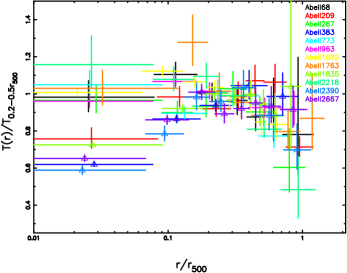
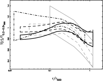
Figure 2: Left: Scaled radial temperature profiles for the pilot LoCuSS sample. The CCCs are in triangles. See the electronic edition of the Journal for a color version. Right: An average temperature profile of the pilot LoCuSS sample (black, solid) compared to the temperature profile ranges in Markevitch et al. (1998, grey, solid), Vikhlinin et al. (2005, grey, dashed), Zhang et al. (2006, black, dashed) and Pratt et al. (2007, black, dash-dotted).

We scaled the radial temperature profiles by $T_{0.2-0.5r_{500}}$ and $r_{500}$ (Fig. 2). Within $0.2r_{\rm 500}$, we observed a temperature drop to at least 70% of the maximum value towards the cluster center for 4 clusters (defined as the CCCs) and an almost constant temperature distribution for the non-CCCs. Previous observations have shown that temperature measurements on scales below $0.2r_{500}$ tend to show peculiarities linked to the cluster dynamical history. For example, the temperatures of merger clusters can be boosted (Smith et al. 2005). However, the boosting is serious mainly in the cluster cores. Using global temperatures excluding the $<0.2r_{500}$ regions can thus (1) tight the scaled profiles of the X-ray properties, (2) minimize the scatter in the X-ray scaling relations and (3) reach a better agreement in the normalization between the X-ray scaling relations for the CCCs and non-CCCs.

An average temperature profile region is derived by averaging the 1-$\sigma$ boundary of the scaled radial temperature profiles. The average temperature profile for the whole sample gives $T(r)\propto r^{0.21\pm 0.04}$, and for the CCC subsample $T(r)\propto r^{0.38\pm 0.04}$, respectively, in the $r<0.2r_{500}$ region. Note the segregation could be more pronounced considering the spatial resolution and PFS effects. This temperature behavior in the cluster cores for the CCC subsample is very similar to the behavior for the nearby CCC sample in Sanderson et al. (2006) giving $T(r)\propto r^{0.4}$ based on Chandra observations. In the outskirts ($0.2r_{500}<r<r_{500}$), the whole sample shows a self-similar behavior giving $T(r)\propto r^{-0.36\pm 0.18}$ with scatter within 20%. A temperature profile decreasing down to 80% of the maximum value with an intrinsic scatter of $\sim 20$% has been observed at about $r_{\rm 500}$ for the average of the sample.

Studies of the cluster temperature distributions (e.g. Markevitch et al. 1998; De Grandi & Molendi 2002; Vikhlinin et al. 2005; Zhang et al. 2004a, 2006; Pratt et al. 2007) indicate a universal temperature profile with a significant decline beyond an isothermal center. The average temperature profile of the pilot LoCuSS sample is consistent with the average profiles from ASCA in Markevitch et al. (1998), BeppoSAX in De Grandi & Molendi (2002) and XMM-Newton in Zhang et al. (2004a, 2006) and Pratt et al. (2007), but is slightly less steep than the profile from Chandra (using an assumed uncertainty of 20% of the averaged temperature profile as an approximate illustration) in Vikhlinin et al. (2005). A similarly universal temperature profile is indicated in outskirts of clusters by simulations (e.g. Borgani et al. 2004; Borgani 2004).

4.2 Scaled metallicity profiles

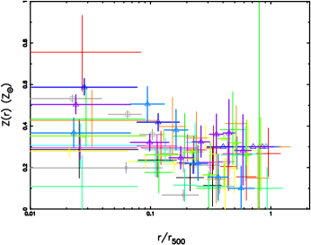
Figure 3: Scaled metallicity profiles. The values in the last bins for some clusters are fixed to 0.3 $Z_{\odot}$ in the spectral fitting which have no error bars. The CCCs are in triangles. The colors have the same meaning as those in Fig. 2. Open and filled boxes denote the average of the scaled metallicity profiles of the CCCs and non-CCCs, respectively, in De Grandi & Molendi (2002, grey).

The metallicity profiles are shown in Fig. 3 with their radii scaled to $r_{500}$. We observed metallicity peaks towards the cluster centers within 0.2 $r_{500}$ for the CCCs. There is no evident evolutionary effect comparing the pilot LoCuSS sample to the nearby CCCs in De Grandi & Molendi (2002) within the measure uncertainties.

4.3 Scaled surface brightness profiles

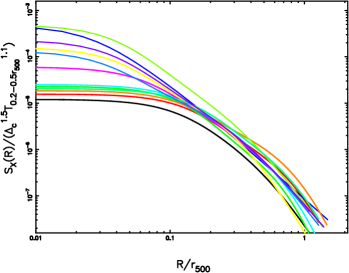
Figure 4: Surface brightness profile fits scaled according to the empirical scaling, $S_{\rm X}\propto T^{1.1}$. The colors have the same meaning as those in Fig. 2.

In the standard self-similar model, gas mass scales with mass and thus temperature as $M_{\rm gas}\propto M\propto T^{1.5}$, which gives $S_{\rm X}\propto T^{0.5}$ (e.g. Arnaud et al. 2002). The $S_{\rm X}$–$T$ scaling based on the empirical $M_{\rm gas}$–$T$ relation provides the least scatter in the scaled surface brightness profiles (e.g. Neumann & Arnaud 2001; Arnaud et al. 2002). We thus applied the current empirical relation $M_{\rm gas}\propto T^{1.8}$ (e.g. Mohr et al. 1999; Vikhlinin et al. 1999; Castillo-Morales & Schindler 2003) corresponding to the scaling $S_{\rm X}\propto T^{1.1}$ to scale the surface brightness profiles (Fig. 4). We found a less scattered self-similar behavior at $R>0.2r_{500}$ for the scaled surface brightness profiles compared to the profiles scaled by $S_{\rm X}\propto T^{0.5}$.

The bolometric X-ray luminosity (here we use the 0.01–100 keV band) is given by $L_{\rm bol}\propto\int\widetilde{\Lambda}(r)n^{2}_{\rm e}(r)dV$, practically an integral of the X-ray surface brightness to 2.5$r_{500}$ ($L_{\rm bol}^{\rm incc}$ in Table2). The value 2.5$r_{500}$ is used because that the extrapolated virial radii are about 2.2–2.6$r_{500}$. We note the luminosity only varies within 3% setting the truncation radius to the value from $r_{500}$ to $2.5r_{500}$.

The surface brightness profiles show small core radii for the CCCs and large core radii for the non-CCCs. Similar to the REFLEX-DXL sample (Zhang et al. 2006) the core radii populate a broad range of values up to 0.2 $r_{500}$. The X-ray luminosity is sensitive to the presence of the cool core. It can thus be used to probe the evolution of the cool cores. We present the bolometric luminosity including and excluding the $R<0.2r_{500}$ region ($L_{\rm bol}^{\rm incc}$ and $L_{\rm bol}^{\rm excc}$) in Table 1. The fractions of the X-ray luminosity attributed to the $R<0.2r_{500}$ region span a broad range up to 70%. This introduces large uncertainties in the use of the luminosity $L_{\rm bol}^{\rm incc}$ as a mass indicator. The normalization varies with the fraction of the CCCs in the sample and the significance of their cool cores by a factor of 30–70%. The X-ray luminosity excluding the $<0.2r_{500}$ region ($L_{\rm bol}^{\rm excc}$) is much less dependent on the presence of the cool core. However, to better re-produce the cluster luminosity and the normalization of the luminosity–temperature/mass relation, we use the X-ray luminosity corrected for the cool core by assuming $S_{\rm X}(R)=S_{\rm X}(0.2r_{500})$ for the $R<0.2r_{500}$ region ($L_{\rm bol}^{\rm corr}$ in Table 1). Using $L_{\rm bol}^{\rm corr}$ for the X-ray scaling relations we obtained reduced scatter and consistent normalization for the CCCs and non-CCCs as shown later. Note the luminosity is lower (by up to 10%) assuming a constant luminosity in the cluster core instead of a beta model, especially for the pronounced CCCs. However, the luminosity corrected for the cool core by the beta model still introduces relatively significant scater dominated by the CCCs due to the correlation between the core radius and the slope parameter.

4.4 Scaled cooling time profiles

The cooling time is derived by the total energy of the gas divided by the energy loss rate

$$t_{\rm c}=\frac{2.5n_{\rm g}T}{n_{\rm e}^{2}\widetilde{\Lambda}}$$ (5)

where $\widetilde{\Lambda}$, $n_{\rm g}$, $n_{\rm e}$ and $T$ are the radiative cooling function, gas number density, electron number density and temperature, respectively. We compute the upper limit of the age of the cluster as an integral from the cluster redshift $z$ up to $z=100$. Cooling regions are those showing cooling time less than the upper limit of the cluster age. The boundary radius of such a region is called the cooling radius. The cooling radius is zero when the cooling time in the cluster center is larger than the upper limit of the cluster age. The cooling time at the resolved inner most radii of the surface brightness profiles and cooling radii are given in Table 2.

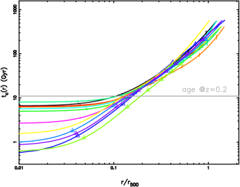
Figure 5: Cooling time profiles. The CCCs are in triangles. The horizontal line denotes the age of the Universe at $z\sim 0.2$. The colors have the same meaning as those in Fig. 2.

In Fig. 5, we show the cooling time profiles with their radii scaled to $r_{500}$. The CCCs show larger cooling radii in unit of $r_{500}$. In the cluster centers, the cooling time is all shorter than the upper limit of the cluster age. The CCCs show much shorter cooling time than for the non-CCCs. The scaled cooling time profiles show a self-similar behavior above $0.2r_{500}$ for the CCC and non-CCC subsamples, respectively. The best fit power law above $0.2r_{500}$ gives $t_{\rm c}(r)\propto r^{1.61\pm 0.01}$ for the whole sample. For the 4 CCCs, the best fit power law above $0.2r_{500}$ gives $t_{\rm c}(r)\propto r^{1.70\pm 0.01}$. For the non-CCCs, the best fit power law above $0.2r_{500}$ is more flat, $t_{\rm c}(r)\propto r^{1.54\pm 0.01}$. The central cooling time is similar to the work in Bauer et al. (2005) using the Chandra data for the same clusters towards the most inner bin resolved. For the pilot LoCuSS sample, the slope of the cooling time profile within 0.2$r_{500}$ becomes steeper with increasing significance of the cool core. This was also observed for the nearby clusters based on Chandra data in Sanderson et al. (2006) and Dunn & Fabian (2006).

The cooling time is calculated towards the cluster center to the inner most bin that the surface brightness profile is resolved. There can be large uncertainties in the cooling time at the inner most bins where the temperature measurements are not resolved. We note that the spatial resolution is important to calculate the proper cooling time in the cluster center. When the cluster core is not well resolved, the value calculated from the measured temperature and electron number density gives the upper limit of the cooling time, specially for the CCCs showing cusped surface brightness profiles.

4.5 Scaled entropy profiles

The entropy is the key to the understanding of the thermodynamical history since it results from shock heating of the gas during cluster formation. The observed entropy is generally defined as $S=Tn_{\rm e}^{-2/3}$ for clusters (e.g. Ponman et al. 1999). Radiative cooling can raise the entropy of the ICM (e.g Pearce et al. 2000) or produce a deficit below the scaling law (e.g. Lloyd-Davies et al. 2000). For all 12 galaxy clusters, the temperature data points are resolved below $0.1r_{500}$. The entropy at $0.1r_{200}$, $S_{\rm 0.1r_{200}}$, can thus be used as an indicator of the central entropy.

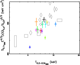
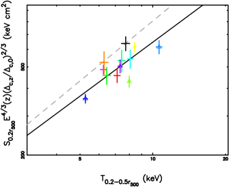
Figure 6: Entropy at $0.1r_{\rm 200}$ (left) and $0.2r_{\rm 500}$ (right) vs. temperature for the pilot LoCuSS sample (crosses) in which the CCCs are in triangles. Nearby clusters in Ponman et al. (2003, boxes) and the REFLEX-DXL sample (diamonds) are shown for comparison. The lines denote the best fits for the pilot LoCuSS sample (solid) and the REFLEX-DXL sample in Zhang et al. (2006, dashed). The colors have the same meaning as those in Fig. 2.

According to the standard self-similar model the entropy scales as $S\propto T$ (e.g. Ponman et al. 1999). We investigated the entropy–temperature relation ($S$–$T$) using $S_{\rm 0.1r_{200}}$ as the central entropy and $T_{0.2-0.5r_{500}}$ as the cluster temperature. $S_{\rm 0.1r_{200}}$ indicates the physics on core scales and $T_{0.2-0.5r_{500}}$ on global scales. Therefore the CCCs show significantly lower central entropies compared to the $S$–$T$ scaling law. This can be due to that lower temperature systems show more pronounced cool cores corresponding to lower central entropies. The entropy at $0.1r_{200}$ can thus be used as a mechanical educt of the non-gravitational process which introduces large scatter of the $S_{\rm 0.1r_{200}}$–$T$ relation (left panel of Fig. 6).

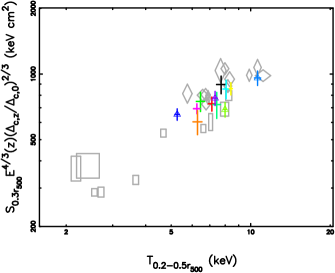
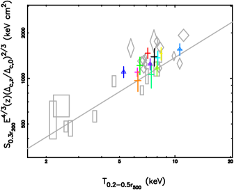
Figure 7: Entropy at $0.3r_{\rm 500}$ (left) and $0.3r_{\rm 200}$ (right) vs. temperature for the pilot LoCuSS sample (crosses), the REFLEX-DXL sample (diamonds) and the sample in Pratt et al. (2006, boxes). The line denote the best fit in Pratt et al. (2006, including only the $E(z)$ correction). The pilot LoCuSS CCCs are in triangles. The colors have the same meaning as those in Fig. 2.

Ponman et al. (2003) suggested to scale the entropy as $S\propto T^{0.65}$ based on the observations for nearby clusters, with which the pilot LoCuSS sample agrees (see the left panel in Fig. 6). $0.1r_{200}$ is slightly smaller than $0.2r_{500}$ for the LoCuSS sample. To avoid the extrapolation to calculate $r_{200}$, we also used the entropies at $0.2r_{500}$, $S_{\rm 0.2r_{500}}$. The scatter is reduced by almost a factor of 2 for the $S$–$T$ relation using $S_{\rm 0.2r_{500}}$ instead of $S_{\rm 0.1r_{200}}$ because that the entropy profiles are more self-similar beyond $0.2r_{500}$ than in the cluster cores. We show the $S$–$T$ relation using $S_{\rm 0.2r_{500}}$ in the right panel of Fig. 6 and Table 5. Within the error, the $S_{\rm 0.2r_{500}}$–$T$ relations for the pilot LoCuSS sample and the REFLEX-DXL sample cannot rule out the standard self-similar model $S\propto T$ while also being consistent with Ponman et al. (2003). The CCCs ($S_{\rm 0.2r_{500}}\propto T^{0.71\pm 0.21}$) agree better with the empirically determined scaling (Ponman et al. 2003) $S\propto T^{0.65}$. As shown in Fig. 7, the further away from the cluster center, the less scatter there is in the $S$–$T$ relation (also see Pratt et al. 2006). There is no noticable evolution in the $S$–$T$ relation (e.g. using $S_{\rm 0.3r_{500}}$ and $S_{\rm 0.3r_{200}}$) comparing the pilot LoCuSS sample to the REFLEX-DXL sample ($z\sim 0.3$, Zhang et al. 2006) and the nearby relaxed cluster sample in Pratt et al. (2006). With the redshift correction, the combined fit of the pilot LoCuSS sample, the REFLEX-DXL sample and the nearby relaxed cluster sample in Pratt et al. (2006) gives $S_{\rm 0.3r_{500}}\propto T^{0.93\pm 0.06}$ and $S_{\rm 0.3r_{200}}\propto T^{0.84\pm 0.08}$, respectively. Note there is the segregation between the CCCs and non-CCCs in which the CCCs show low normalization of the $S$–$T$ relation. With the combined data, at the high mass end the clusters are un-biased to CCCs and at the low mass end the clusters are biased to CCCs (relaxed clusters in Pratt et al. 2006). The slope of the $S$–$T$ relation for the combined data is thus steeper than the slope for the CCCs or non-CCCs. This is less significant for the $S$–$T$ relation using the entropies at larger radii, e.g. $S_{\rm 0.3r_{200}}$.

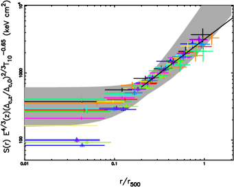
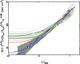
Figure 8: Left: Scaled entropy profiles for the pilot LoCuSS sample and the combined best fit. The shadow denotes the range of the entropy profiles of the nearby clusters in the same temperature range in Ponmen et al. (2003). Right: Scaled entropy profile fits for the pilot LoCuSS sample compared to the REFLEX-DXL sample in Zhang et al. (2006, grey, thin) and the sample in Pratt et al. (2006, black, hatched). The CCCs are in triangles. $T_{10}$ denotes $T_{0.2-0.5r_{500}}/10$ keV. The colors have the same meaning as those in Fig. 2.

We scaled the radial entropy profiles using the empirically scaling (Ponman et al. 2003) $S\propto T^{0.65}$ and $r_{500}$. As shown in Fig. 8, the scaled entropy profiles for the pilot LoCuSS sample are self-similar above $0.2r_{500}$ and show the least scatter around 0.2–0.3$r_{500}$. However, we found the redshift correction is required to obtain an agreement on global radial scales for the pilot LoCuSS sample, Birmingham-CfA sample (Ponman et al. 2003), REFLEX-DXL sample (Zhang et al. 2006) and the cluster sample in Pratt et al. (2006).

After the redshift correction the combined entropy profiles of the pilot LoCuSS sample give the best fit $S(r)\propto r^{1.01\pm 0.04}$ above $0.2r_{\rm 500}$. A similar power law was found as $S\propto r^{0.97}$ by Ettori et al. (2002), $S\propto r^{0.95}$ by Piffaretti et al. (2005), and $S(r)\propto r^{1.00\pm 0.07}$ for the REFLEX-DXL sample ($>0.2r_{500}$). The spherical accretion shock model predicts $S\propto r^{1.1}$ (e.g. Tozzi & Norman 2001; Kay 2004). The combined fit of the entropy profiles for the 4 CCCs in the pilot LoCuSS sample gives $S\propto r^{1.10\pm 0.05}$, similar to the prediction of the spherical accretion shock model and consistent with the relaxed nearby clusters in Pratt et al. (2006) giving $S\propto r^{1.08}$. Since the clusters appear more “relaxed” in Pratt et al (2006) the entropy profiles of their sample are very consistent with the CCCs in the pilot LoCuSS sample. The combined fit of the entropy profiles for the 8 non-CCCs in the pilot LoCuSS sample gives $S\propto r^{0.97\pm 0.05}$.

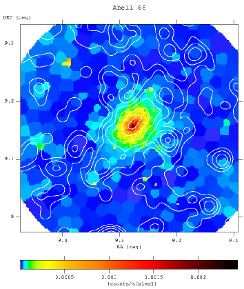
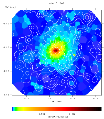
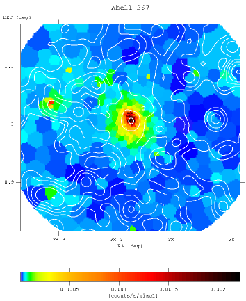
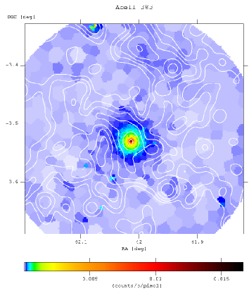
Figure 17: Flat fielded XMM-Newton MOS1 flux images in the 0.7–2 keV band superposed with the CFH12k optical luminosity weighted galaxy density contours.

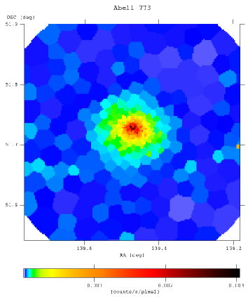
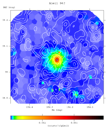
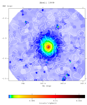
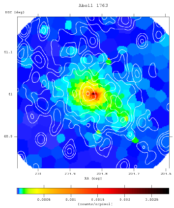
Figure 24: See the caption in Fig. 17. Abell 773 has no CFH12k data.

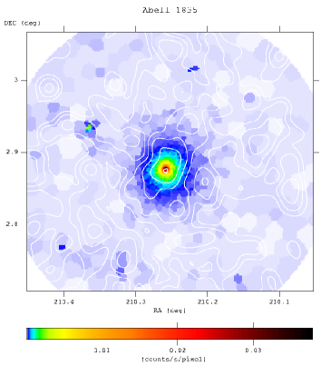
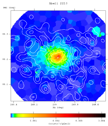
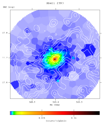
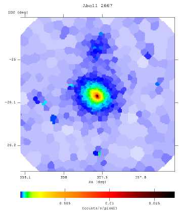
Figure 25: See the caption in Fig. 17. Abell 2667 has no CFH12k data.

The different slopes of the entropy profiles for the CCCs and non-CCCs may indicate the different phases or different origins of the clusters with respect to the cluster morphologies. Observations suggest an evolution of the cluster morphology such that mergers happen more frequently in high redshift galaxy clusters (e.g. Jeltema et al. 2005; Hashimoto et al. 2006). The non-CCCs are dynamically young and thus show the evidence of the recent mergers judging from their X-ray flux images such as elongation and extended low surface brightness features (e.g. Abell 1763 in the pilot LoCuSS sample). Their entropy profiles can be flattened by mergers and thus become less steep than the prediction of the spherical accretion shock model. There is an evidence of AGN activities in some clusters (e.g. Abell 1763, Hardcastle & Sakelliou 2004), in which the central AGN could also affect the entropy profile. On the contrary, the CCCs appear “relaxed”, and their entropy profiles agree with the prediction of the spherical accretion shock model. On the other hand, the different slopes of the entropy profiles of the CCCs and non-CCCs can also be due to geometry. The non-CCCs appear more elongated due to the recent mergers while the CCCs more symmetric as shown in the XMM-Newton flux images (Fig. 17, also see Figs. 24–25 in the electronic edition of the Journal for the whole sample). The flattening of the entropy profiles of the non-CCCs can also be a geometric effect due to the azimuthal average.

4.6 Scaled total mass and gas mass profiles

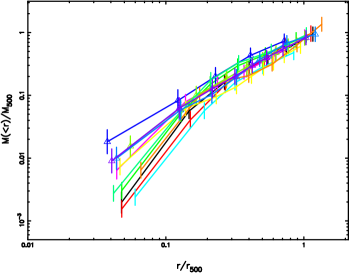
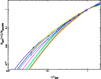
Figure 9: Scaled total mass profiles (left) and gas mass profiles (right). The CCCs are in triangles. The colors have the same meaning as those in Fig. 2. The error bars (a few per cent) of the gas mass profiles are too small to be seen in this plot.

The mass profiles were scaled with respect to $M_{\rm 500}$ and $r_{\rm 500}$, respectively (Fig. 9). We found the least scatter at radii above $0.2r_{\rm 500}$. In the inner regions ($<0.2r_{\rm 500}$), the mass profiles vary significantly with the cluster central dynamics (Fig. 9). As found in the strong lensing studies based on high quality HST data (Smith et al. 2005), the cluster cores can be very complicated with multi-clump DM halos. The peculiarities in the cluster cores for the individual clusters may explain the large scatter of the mass profiles on core scales where the ICM does not always trace DM. This scatter may also suggest the different phases of the clusters.

Similar to the mass profiles, the scaled gas mass profiles appear self-similar at radii above $0.2r_{\rm 500}$ but show less scatter (a few per cent) than for the scaled mass profiles.

5 X-ray scaling relations

To use the mass function of the cluster sample to constrain cosmological parameters, it is important to calibrate the scaling relations between the X-ray luminosity, temperature and gravitational mass, the fundamental cluster properties including also velocity dispersion. Massive clusters, selected in a narrow redshift range are important to constrain the normalization and to understand the scatter in the scaling relations. Both REFLEX-DXL and pilot LoCuSS samples are such flux-limited, morphology unbiased samples. Comparing the X-ray scaling relations of such samples to samples in other narrow redshift bins can constrain the evolution of the X-ray scaling relations.

The scaling relations are generally parameterized by a power law ($Y=Y_{0}X^{\gamma}$). Note the pilot LoCuSS clusters are in a narrow temperature range, which has the disadvantage to constrain the slope parameter. To study the normalization segregation of the scaling relations for the CCCs and non-CCCs, we fit the normalization with fixed slope parameters as often used in previous studies for the pilot LoCuSS sample and the pilot LoCuSS non-CCCs. For each relation, we also performed the fitting with both normalization and slope free. The fitting slopes generally appear consistent with the fixed slopes within the errors. The scatter describes the dispersion between the observational data and the best fit. We list the best fit power law and the scatter in Table 5. For the pilot LoCuSS sample the cluster masses are uniformly determined from high quality XMM-Newton data. This guarantees the minimum systematic error due to the analysis method.

5.1 Cool cores and the X-ray scaling relations

In the cluster cores we observed broad scatter of the X-ray properties with respect to the cluster morphologies (e.g. CCCs and non-CCCs) for the scaled profiles of the X-ray quantities (e.g. temperature, metallicity, surface brightness, cooling time, entropy, total mass and gas mass). This is most probably due to the effects of different physical processes rather than statistical fluctuations in the measurements (Zhang et al. 2004b, 2005b; Finoguenov et al. 2005). The CCCs and non-CCCs can be the clusters at their different phases.

The X-ray luminosity integrated over the whole cluster region introduces significant normalization segregation between CCCs and non-CCCs, and large scatter of the X-ray scaling relations dominated by non-CCCs. It is thus worth to take a closer look how the cool cores affect the scaling relations and their scatter as follows.

For $S_{0.1r_{200}}$–$T$ relation, including the CCCs in the sample introduces not only a steeper slope but also a lower normalization ($\sim 30$%).

Using the X-ray luminosity including the cool core ($L^{\rm incc}$), the normalization of the $L$–$T$ and $L$–$M$ relations excluding the 4 CCCs is reduced by 40%. If the temperature is measured also including the cool core, the normalization segregation will be even larger (by a few per cent) for the $L$–$T$ relation. Using the luminosity corrected for the $<0.2r_{500}$ region and temperature excluding the $<0.2r_{500}$ region, the normalization of the scaling relations agrees to better than 10% for the CCCs and non-CCCs. In such a way the scaling relations among X-ray luminosity, cluster mass and temperature, and their scatter are insensitive to the exclusion of CCCs for the pilot LoCuSS sample. The above results show the following picture. CCCs usually appear more “relaxed”, and are thus considered to provide reliable X-ray mass measurements (e.g. Pierpaoli et al. 2001; Allen et al. 2004). At the same time, the properties of the cool cores exhibit the largest scatter. Therefore, the CCCs were usually selected and the cool cores were often excised or corrected to study the X-ray scaling relations.

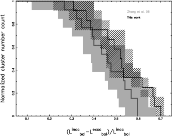
Figure 10: Normalized cumulative cluster number count as a function of the fraction of the total bolometric luminosity attributed by the $<0.2r_{500}$ region for the pilot LoCuSS sample at $z\sim 0.2$ compared to the REFLEX-DXL sample at $z\sim 0.3$ in Zhang et al. (2006).

With the bolometric X-ray luminosity including and excluding the $<0.2r_{500}$ region (Table 2), we show the normalized cumulative cluster number count as a function of the fraction of the luminosity attributed by the cluster core ($<0.2r_{500}$) in Fig. 10. Up to 70% of the bolometric X-ray luminosity is contributed by the cluster core ($<0.2r_{500}$). The evolution of the cool cores is not significant as also explained using the temperature drop towards the cluster center in Sect. 3.2.

As mentioned above the global temperature was calculated excluding the $<0.2r_{500}$ region and the X-ray luminosity was corrected for the $<0.2r_{500}$ region, respectively. In such a way the scatter in the X-ray scaling relations is minimized ($<20$%) and the normalization of the X-ray scaling relations is insensitive to the exclusion of the CCCs ($<10$%).

5.2 Mass–temperature relation

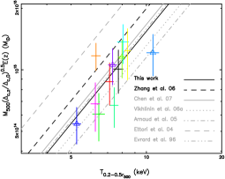
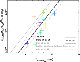
Figure 11: Mass temperature relation (left) and gas mass temperature relation (right). The CCCs are in triangles. The colors have the same meaning as those in Fig. 2. The best fit power law of the pilot LoCuSS sample and REFLEX-DXL sample used the fixed slope of 1.5 for the $M$–$T$ relation and 1.8 for the $M_{\rm gas}$–$T$ relation.

Given the virial theorem ($T\propto M_{500}/r_{500}$) and the spherical collapse model ($M_{500}\propto r_{500}^{3}$) one obtains $M_{500}\propto T^{1.5}$. This scaling was also observed for nearby clusters (e.g. Finoguenov et al. 2001; Reiprich & Böhringer 2002; Arnaud et al. 2005). To compare the pilot LoCuSS sample to the existing nearby and more distant samples, we present the $M_{500}$–$T$ relation fixing the slope parameter to the often used value (1.5) in Fig. 11. The scatter in the cluster mass in the $M_{500}$–$T$ relation is within 20% for the pilot LoCuSS sample.

Evrard et al. (1996) simulated ROSAT observations of 58 nearby clusters ($z\sim 0.04$, 1–10 keV), for which the normalization of the $M$–$T$ relation agrees with the pilot LoCuSS sample. Chen et al (2007) investigated ROSAT and ASCA observations of a flux-limited, morphology-unbiased sample of 106 nearby clusters ($z<0.15$, 1–15 keV, extended HIFLUGCS). The scaling relation of the massive non-CCCs ($T>3$ keV) in their sample shows an excellent agreement with the pilot LoCuSS sample. This also indicates that the cool core correction for the pilot LoCuSS sample introduces less bias into the normalization towards the CCCs. Note the early work related to the HIFLUGCS sample (Finoguenov et al. 2001; Popesso et al. 2005) gives similar scaling relations as in Chen et al. (2007) for the whole HIFLUGCS sample. Vikhlinin et al (2006a) derived the $M$–$T$ relation for 13 low-redshift clusters ($z<0.23$, 0.7–9 keV) using Chandra observations, which normalization agrees with ours within the scatter (20%) for the pilot LoCuSS sample. The scaling in Arnaud et al. (2005) is based on XMM-Newton observations of 6 relaxed nearby clusters ($z<0.15$, 2–9 keV, $T>3.5$ keV). The temperatures used in their work were determined in the 0.1–0.5$r_{200}$ region, which also excludes the cluster cores as we did using the 0.2–0.5$r_{500}$ region. The temperature profiles in Arnaud et al. (2005) are almost flat in the $0.5r_{500}$–$0.5r_{200}$ regions and their values are close to the maximum temperatures. The measured global temperature is thus higher when the $0.5r_{500}$–$0.5r_{200}$ region is used as in Arnaud et al. (2005) than the global temperature measured excluding the $0.5r_{500}$–$0.5r_{200}$. We, also in Zhang et al. (2006), measured the global temperatures using the region only up to $0.5r_{500}$ determined by the photon statistic. Therefore the normalization of the $M$–$T$ scaling relations in this work and Zhang et al. (2006) is slightly higher than in Arnaud et al. (2005).

The $M$–$T$ relation in Ettori et al. (2004) is based on Chandra observations of 28 high redshift clusters ($0.4<z<1.3$, 3–11 keV). It shows a higher normalization compared to the above published relations we mentioned. This could be due to the different way to define the density contrast used in the redshift evolution correction and the method to calculate the global temperatures in Ettori et al. (2004). We used the redshift dependent density contrast (Bryan & Norman 1998) in the redshift evolution correction. We note that in this work the cool cores are excluded in calculating the global temperatures. In Ettori et al. (2004) the central regions including cluster cool cores were used to measure the global temperatures, which tends to give lower temperatures for given cluster masses for the clusters showing cool cores. Therefore the normalization of the $M$–$T$ relation in Ettori et al. (2004) can be higher. The scaling relation in Zhang et al. (2006) is based a flux-limited morphology-unbiased sample of 13 medium distant clusters ($0.26<z<0.31$, $T>5$ keV, REFLEX-DXL) observed by XMM-Newton. Compared to the sample in this work the REFLEX-DXL sample shows a slightly higher normalization but well within the mass scatter ($\sim 20$%) for the pilot LoCuSS sample.

No evident evolution is found for the $M$–$T$ relation comparing the pilot LoCuSS sample to the nearby and more distant samples within the scatter.

5.3 Gas mass–temperature relation

Assuming the gravitational effect dominates in galaxy clusters, the gas should follow the collapse of the DM giving $M_{\rm gas,500}\propto M_{500}$ and thus $M_{\rm gas,500}\propto T^{1.5}$ (e.g. Arnaud 2005). However, the non-gravitational effects become important for the ICM such that the shape of the ICM density profile depends on the cluster temperature (e.g. Ponman et al. 1999) and the observed slope of the $M_{\rm gas,500}$–$T$ relation becomes steep ($\sim 1.8$, e.g. Mohr et al. 1999; Vikhlinin et al. 1999). The slope of the gas mass–temperature relation for the pilot LoCuSS sample is consistent with the previously observed value 1.8 within the error. Therefore, we present the $M_{\rm gas,500}$–$T$ relation for the pilot LoCuSS sample with the fixed slope of 1.8 to compare with the recently published results in Fig. 11. The scatter of the gas mass for the $M_{\rm gas,500}$–$T$ relation is within 15% for the pilot LoCuSS sample. Note the weighted (unweighted) fitting slope of the $M_{\rm gas,500}$–$T$ relation is $2.8\pm 0.8$ ($1.6\pm 0.2$).

The $M_{\rm gas,500}$–$T$ relation in Mohr et al. (1999) is based on a flux-limited sample of 45 nearby clusters spanning a temperature range of 2–10 keV observed by ROSAT and ASCA. Castillo-Morales & Schindler (2003) investigated a sample of 10 nearby clusters ($0.03<z<0.09$, 4.7–9.4 keV) also observed by ROSAT and ASCA. The $M_{\rm gas,500}$–$T$ relation for the pilot LoCuSS sample agrees with the published relations for (i) the nearby samples in e.g. Mohr et al. (1999), Castillo-Morales & Schindler (2003), and Chen et al. (2007, the non-CCCs with $T>3$ keV in HIFLUGCS), and (ii) the more distant sample in Zhang et al. (2006, REFLEX-DXL).

5.4 Luminosity–temperature relation

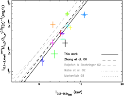
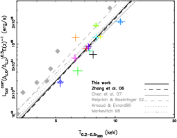
Figure 12: X-ray luminosity in the 0.1–2.4 keV band vs. temperature (left) and bolometric luminosity vs. temperature (right). The CCCs are in triangles. The clusters in Kotov & Vikhlinin (2005) are in diamonds. The colors have the same meaning as those in Fig. 2. The best fit power law of the pilot LoCuSS sample and REFLEX-DXL sample used the fixed slope of 2.6 for the $L_{\rm 0.1-2.4keV}^{\rm corr}$–$T$ relation and 2.98 for the $L_{\rm bol}^{\rm corr}$–$T$ relation.

In the standard self-similar model $M_{\rm gas,500}\propto M_{500}\propto T^{1.5}$ and $M_{500}\propto r_{500}^{3}$ give $L\propto M_{\rm gas}^{2}T^{0.5}/r_{500}^{3}\propto T^{2}$. However, the $L$–$T$ relation deviates from the $L\propto T^{2}$ scaling due to the dependence of the ICM distribution on the cluster temperature (e.g. Neumann & Arnaud 2001) and becomes steeper. Given the empirical scaling $M_{\rm gas,500}\propto T^{1.8}$, one gets $L\propto T^{2.6}$ as often found in observations. We thus fixed the slope to the often observed values (e.g. 2.6 for $L_{\rm 0.1-2.4keV}^{\rm corr}$–$T$ and 2.98 for $L_{\rm bol}^{\rm corr}$–$T$, e.g. observed in Reiprich & Böhringer 2002), and compared the findings for the pilot LoCuSS sample to the recent results in Fig. 12. For the pilot LoCuSS sample, the scatter of the luminosity for the $L$–$T$ relations is within 15%.

The $L$–$T$ relation has been intensively studied for the nearby cluster samples using the luminosity based on ROSAT observations and the temperature based on ASCA observations, for example, in (i) Markevitch (1998, 30 clusters, $0.04<z<0.09$, $T>3.5$ keV), (ii) Evrard & Arnaud (1999, 24 clusters, $z<0.37$, $T>2$ keV), (iii) Reiprich & Böhringer (2002, in which the flux-limited morphology-unbiased sample HIFLUGCS was initially constructed and investigated, note the fits are for the whole HIFLUGCS sample including groups), (iv) Ikebe et al. (2002, a flux-limited sample of 62 clusters, $z<0.16$, 1–10 keV), and (v) Chen et al. (2007, HIFLUGCS).

The $L$–$T$ relation deviates from the standard self-similar prediction $L\propto T^{2}$, but shows no evolution comparing the pilot LoCuSS sample to the nearby samples in Markevitch (1998) and Arnaud & Evrard (1999) using representative non-CCCs. As flux-limited morphology-unbiased samples, the $L^{\rm corr}_{\rm 0.1-2.4keV}$–$T$ relation for the pilot LoCuSS sample agrees with the HIFLUGCS sample (e.g. Reiprich & Böhringer 2002, including groups; Chen et al. 2007, non-CCCs with $T>3$ keV), the sample in Ikebe et al. (2002) and the REFLEX-DXL sample (e.g. Zhang et al. 2006). Therefore no evident evolution is observed for the $L$–$T$ relation up to redshift 0.3.

Kotov & Vikhlinin (2005) applied an alternative redshift evolution for the $L$–$T$ relation of 10 distant non-CCCs ($0.4<z<0.7$, $T>3.5$ keV), giving $L\propto T^{2.64}(1+z)^{1.8}$. We applied the redshift correction to the 7 clusters available in Kotov & Vikhlinin (2005) also observed by XMM-Newton and found an agreement with the pilot LoCuSS sample within the scatter. We note that in Kotov & Vikhlinin (2005) the temperature was measured in the 70 kpc–$r_{500}$ region and luminosity in the 70–1400 kpc region, in which a small central region was excluded in calculating the temperature/luminosity. This tends to give slightly lower/higher temperature/luminosity and thus higher normalization of the $L$–$T$ relation compared to the pilot LoCuSS sample. On the other hand, Kotov & Vikhlinin (2005) used the same aperture for the correction which gives a more significant correction of the cool core for a less massive system and could thus provide lower normalization of the $L$–$T$ relation for less massive systems.

5.5 Luminosity–mass relation

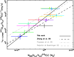
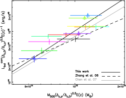
Figure 13: X-ray luminosity in the 0.1–2.4 keV band vs. total mass (left) and bolometric luminosity vs. cluster total mass (right). The CCCs are in triangles. The colors have the same meaning as those in Fig. 2. The best fit power law of the pilot LoCuSS sample used the fixed slope of 1.73 for the $L_{\rm 0.1-2.4keV}^{\rm corr}$–$M$ relation and 1.99 for the $L_{\rm bol}^{\rm corr}$–$M$ relation. The fixed slope of 1.3 was used for the REFLEX-DXL sample in Zhang et al. (2006).

With $M\propto T^{1.5}$ and $L\propto T^{2}$ in the standard self-similar model one derives $L\propto M^{1.33}$. With the observed scaling relations in e.g. Reiprich & Böhringer (2002), $L_{\rm 0.1-2.4keV}\propto T^{2.6}$ gives $L_{\rm 0.1-2.4keV}\propto M^{1.73}$ and $L_{\rm bol}\propto T^{2.98}$ gives $L_{\rm bol}\propto M^{1.99}$, respectively. The fitting of the pilot sample favors the observed scaling relations. Therefore, we fixed the slope to 1.73 for $L_{\rm 0.1-2.4keV}^{\rm corr}$–$T$ and 1.99 for $L_{\rm bol}^{\rm corr}$–$T$, and compared the pilot LoCuSS sample to the recent results in Fig. 13. The scatter of the luminosity and mass for the $L$–$T$ relations is within 15% and 20%, respectively.

The pilot LoCuSS sample agrees with the nearby sample HIFLUGCS (Reiprich & Böhringer 2002; Popesso et al. 2005; Chen et al. 2007, non-CCCs with $T>3$ keV) and the more distant sample REFLEX-DXL (Zhang et al. 2006) also as flux-limited morphology-unbiased samples. Therefore we observed no evident evolution of the luminosity–mass relation.

5.6 $r_{500}$ vs. global temperature

As found in Evrard et al. (1996) the standard self-similar model predicts $r_{500}\propto M^{1/3}\propto T^{0.5}$. The best fit for the pilot LoCuSS sample confirms the standard self-similar model, and gives $r_{500}=10^{-0.335\pm 0.106}T_{0.2-0.5r_{500}}^{0.57\pm 0.12}E(z)^{-1}(\Delta_{c,z}/\Delta_{c,0})^{-0.5}$ Mpc. It agrees with the scaling relation, $r_{500}\propto T^{0.50\pm 0.05}$ for 6 relaxed nearby clusters ($z<0.15$, 2–9 keV, $T>3.5$ keV) in Arnaud et al. (2005) also observed by XMM-Newton.

The above comparison of the X-ray scaling relations in this work with the published results (Figs. 11–13) for the nearby and more distant samples shows that the evolution of the scaling relations can be accounted for by the redshift evolution given in Sect. 4. As shown in Table 5 the normalization of the scaling relations agrees for the CCCs and non-CCCs to better than 10% using the temperature measured excluding the cool core and the luminosity corrected for the cool core. The X-ray quantities such as temperature and luminosity can be used as reliable indicators of the cluster mass with the scatter less than 20%. In general, the slopes of the scaling relations indicate the need for non-gravitational processes. This fits into the general opinion that galaxy clusters show a modified self-similarity up to $z\sim 1$ (e.g. Arnaud 2005). As also demonstrated in simulations (e.g. Poole et al. 2007), mergers only alter the structure of compact cool cores, and the outer structure ($>0.1r_{200}$ or $>0.2r_{500}$) is survived after the merger events. The scaling relations are thus preserved for galaxy clusters.

6 Discussion

6.1 Comparison of the X-ray results

The Chandra data of Abell 1689 (Xue & Wu 2002), Abell 383 and Abell 2390 (Vikhlinin et al. 2006a) were analyzed in details. Bauer et al. (2005) present the cooling time of 8 clusters in the pilot LoCuSS sample based on Chandra data. Smith et al. (2005) measured the Chandra temperatures for 9 clusters in this sample. The published Chandra results for these clusters agree with the XMM-Newton results in this work. We also obtained an agreement with the published results based on the same XMM-Newton data, e.g. Abell 1689 (Andersson & Madejski 2004), Abell 1835 (Majerowicz et al. 2002; Jia et al. 2004) and Abell 2218 (Pratt et al. 2005).

6.2 Gas profiles in the outskirts

The generally adopted $\beta$ model ($\beta=2/3$) gives $n_{\rm e}\propto r^{-2}$. However, Vikhlinin et al. (1999) found a mild trend for $\beta$ to increase as a function of cluster temperature, which gives $\beta\sim 0.80$ and $n_{\rm e}\propto r^{-2.4}$ for clusters around 10 keV. Bahcall (1999) also found that the electron number density scales as $n_{\rm e}\propto r^{-2.4}$ at large radii. Zhang et al. (2006) confirmed their conclusion that $n_{\rm e}\propto r^{-2.42}$ for the REFLEX-DXL clusters. Due to the gradual change in the slope, one should be cautious to use a single slope double-$\beta$ model which might introduce a systematic error in the cluster mass measurements (as also described in e.g. Horner 2001). Similarly, we performed the power law fit of the ICM density distributions at radii above $3^{\prime}$ for the present sample and obtained an average of $n_{\rm e}\propto r^{-2.2\pm 0.1}$.

6.3 Lensing to X-ray mass ratios

Smith et al. (2005) present a uniform strong lensing analysis of 9 clusters in this sample. We took these 9 overlapping clusters as a subsample (hereafter the S05 subsample, X-ray selected) and compared the strong lensing and X-ray masses. Ten clusters in the pilot LoCuSS sample have CFH12k data. The detailed data reduction method can be found in Bardeau et al. (2005) and the weak lensing results of the sample in Bardeau et al. (2006), respectively. The CFH12k optical luminosity weighted galaxy number density contours and weak lensing masses are given in Bardeau et al. (2006). We took these 10 clusters as a subsample (hereafter the B06 subsample, X-ray selected) and compared the weak lensing and X-ray masses. In total eleven clusters have both X-ray and weak/strong lensing masses.

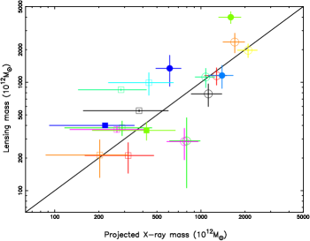
Figure 14: Strong lensing mass vs. projected X-ray mass at $r_{2500}$ for the S05 subsample (boxes) and weak lensing mass vs. projected X-ray mass at $r^{\rm wl}_{200}$ for the B06 subsample (circles), respectively. The symbols for the CCCs are solid. The colors have the same meaning as those in Fig. 2.

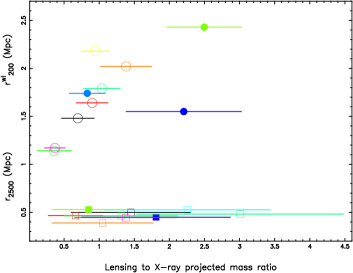
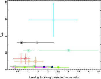
Figure 15: Left: $r_{2500}$ vs. strong lensing to X-ray projected mass ratio for the S05 subsample (boxes) and $r^{\rm wl}_{200}$ vs. weak lensing to X-ray projected mass ratio for the B06 subsample (circles), respectively. Right: substructure fraction (defined in Smith et al. 2005) vs. strong lensing to X-ray projected mass ratio at $r_{2500}$ for the S05 subsample (boxes) and weak lensing to X-ray projected mass ratio at $r^{\rm wl}_{200}$ for the B06 subsample (circles), respectively. The symbols for the CCCs are solid. The colors have the same meaning as those in Fig. 2.

To compare to the lensing mass we calculated the projected X-ray mass distribution for each cluster using its observed radial mass profile. We note that the clusters are detected up to the radii between $r_{500}$ and $r_{200}$. Because the extrapolated virial radii are about 2.2–2.6$r_{500}$, we projected the observational mass profile using a truncation radius of $2.5r_{500}$. We also performed the projection to the weak lensing determined $r^{\rm wl}_{200}$. The comparison of the projected X-ray masses using these 2 different truncation radii, $2.5r_{500}$ and $r^{\rm wl}_{200}$), shows that the X-ray projected mass is insensitive to the truncation radius, varying within a few per cent. The error introduced by the projection to $2.5r_{500}$ is relatively small compared to the projected mass uncertainties, for example, $\sim 30$% at $r^{\rm wl}_{200}$ for Abell 68 using the uncertainties of the electron number density and temperature measurements by Monte Carlo simulations. Therefore we adopt the projected X-ray mass using the truncation radius of $2.5r_{500}$ for further applications. We compare the X-ray masses to the strong lensing masses in Smith et al. (2005) at the X-ray determined $r_{2500}$ and to the weak lensing masses in Bardeau et al. (2006) at the weak lensing determined $r^{\rm wl}_{200}$, respectively (Fig. 14 and Fig. 15). The scatter in the strong/weak lensing to X-ray mass ratio is comparable.

Within the error, 6 out of 9 clusters show consistent mass estimates between X-ray and strong lensing approaches. One third of the clusters show higher strong lensing masses compared to the X-ray masses up to a factor of 2.5. The mean of the strong lensing to X-ray mass ratio is 1.53 with its scatter of 1.07. On average the strong lensing approach tends to give larger masses than the X-ray approach especially for dynamically active clusters.

Within the error, 4 out of 10 clusters show consistent mass estimates between X-ray and weak lensing approaches. The mean of the weak lensing to X-ray mass ratio is 1.12 with its scatter of 0.66. Among the clusters showing inconsistent masses, half have higher weak lensing masses compared to the X-ray masses. On average the X-ray and weak lensing approaches agree better.

6.4 Mass discrepancy

The mass discrepancy between X-ray and lensing can be a combination of the measurement uncertainties and the physics in the individual clusters. The following issues have to be considered in properly comparing the lensing and X-ray masses. (1) Simulations in Poole et al (2006) show that the temperature fluctuations $\Delta T/T\sim 20\%$ can pass the virialization point and persist in the compact cluster cores. Therefore temperature fluctuations at the 20% level do not necessarily indicate a disturbed system, but introduce uncertainties in the cluster mass estimates in the central region. (2) As demonstrated in Puy et al. (2003), the relative error of the X-ray surface brightness goes almost linearly as a function of the rotating angle and axis ratio of the cluster, respectively. The projection of the X-ray masses here is based on the assumption of spherical symmetry, in which the total mass can be easily overestimated/underestimated for aspherical clusters. (3) Specially for the mass distribution in a CCC the cool core has to be well resolved to guarantee the proper X-ray mass estimate in the central region. (4) The line-of-sight merger can enhance the possibility to observe the cluster by strong lensing. A strong lensing selected sample can be boosted because of this. (5) The lack of reliable redshift measurements of the faint galaxies in the weak lensing analysis causes confusion of the lensed background galaxies and unlensed cluster galaxies. This introduces a significant uncertainty in the weak lensing mass estimate (Pedersen et al. 2006). (6) The lack of reliable arc redshift measurements causes uncertainties in the strong lensing mass estimate. (7) The mass distribution of the DM halo can be more complex with multi-components which can significantly affect the strong lensing analysis (e.g. Smith et al. 2005).

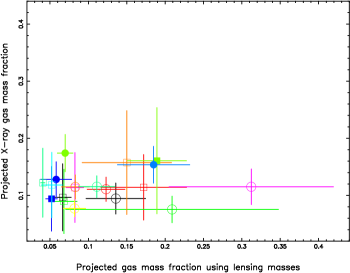
Figure 16: Projected X-ray gas mass fraction vs. projected gas mass fraction using strong lensing (boxes) and weak lensing (circles) masses, for the S05 subsample and B06 subsample, respectively. The symbols for the CCCs are solid. The colors have the same meaning as those in Fig. 2.

The mass discrepancy between X-ray and lensing partially come from the interpretation of galaxy dynamics and ICM structure in galaxy clusters (e.g. Smith et al. 2005; Zhang et al. 2005a). The optical cluster morphology is described in Bardeau et al. (2006). To reveal the link between the X-ray lensing mass discrepancy and the characters of the individual clusters, we investigated the strong/weak lensing to X-ray mass ratio as a function of the X-ray properties such as temperature, metallicity, central entropy, cooling radius, cooling time and X-ray luminosity. However, no evident correlations are observed. This could be a result of the low statistic of only 10 clusters in the subsample. A large sample with better statistic could be helpful for better understanding. In Fig. 16 we present the projected gas mass fractions at $r_{2500}$ using the strong lensing masses and at $r^{\rm wl}_{200}$ using the weak lensing masses, which span a broad range up to 0.3. The scatter of the projected gas mass fractions using the strong (weak) lensing approach is larger by a factor of 1.5 (2.5) than the scatter using the X-ray masses.

Combining data on the optical cluster morphology and the X-ray appearance of the cluster may tell more about the cluster structure and mass discrepancy. The soft band images are less temperature dependent and thus better reflect the ICM density distribution. The MOS1 data show less serious gaps which is important to check the cluster morphology. To have a closer look at the cluster morphology we created flat fielded point source included XMM-Newton MOS1 flux images in the 0.7–2 keV band binned in $8^{\prime\prime}\times 8^{\prime\prime}$. The weighted Voronoi tesselation method (Cappellari & Copin 2003; Diehl & Statler 2006) was used to bin the image to $5\sigma$ significance. In Fig. 17 (also see Figs. 24–25 in the electronic edition of the Journal for the whole sample), we superposed the CFH12k optical luminosity weighted galaxy density contours (Bardeau et al. 2006) on the X-ray adaptively binned images.

6.4.1 Strong lensing and X-ray masses

The morphology of the X-ray images overlaid with optical contours can be used to understand the mass discrepancy in the central regions combined with the substructure fraction in the strong lensing analysis (Smith et al. 2005). We thus present the strong/weak lensing to X-ray mass ratio versus the substructure fraction (Fig. 15). Three clusters show discrepancies of the masses using the strong lensing and X-ray approaches. Here we discuss these 3 clusters, which show a significant link between the substructure fraction and strong lensing to X-ray mass ratio.

Abell 383 has very low substructure fraction, appearing “relaxed” in the strong lensing analysis. The X-ray temperature profile show a strong decrease towards the cluster center, which can be even more significant considering the PSF correction. This can add uncertainties in the X-ray mass estimate.

Abell 773 and Abell 2218 have very high substructure fractions showing multi-modal DM halos as found in Smith et al. (2005). In X-rays the multi-clumps are smeared out and both clusters appear symmetric. This may explain the large mass discrepancy between strong lensing and X-ray for Abell 773 (by a factor of 2.3) and Abell 2218 (by a factor of 3). Reliable arc redshift measurements have been obtained in the strong lensing mass estimate for Abell 2218 (e.g. Smith et al. 2005 and the references in). The mass distribution of the DM halo in Abell 2218 shows a complex structure with multi-components in the central region (Smith et al. 2005). The pronounced mass discrepancy between X-ray and strong lensing for Abell 2218 is mostly due to the combination of (1), (2), (4) and (7) as partly indicated in Girardi et al. (1997) and Pratt et al. (2005).

6.4.2 Weak lensing and X-ray masses

Among the 6 clusters with inconsistent weak lensing and X-ray masses, the mass discrepancy is not significant for Abell 68 and Abell 1763.

The highest projected gas mass fractions were observed in Abell 963 ($\sim 0.3$) and Abell 267 ($\sim 0.2$) using the weak lensing masses (Fig. 16). The X-ray masses are likely reliable for these 2 clusters since both clusters appear regular in their X-ray flux images. Therefore the high projected gas mass fractions using the weak lensing masses may indicate that the weak lensing masses are underestimated for these 2 clusters. This could explain the low weak lensing to X-ray mass ratio ($\sim 0.4$) for Abell 267 and Abell 963.

Abell 1835 shows the most significant mass discrepancy (by a factor of 2.5) between X-ray and weak lensing. At $r^{wl,c02}_{200}=2.11$ Mpc given by the weak lensing analysis in Clowe & Schneider (2002), our X-ray mass is $(10.4\pm 2.1)\times 10^{14}M_{\odot}$, in a good agreement with their weak lensing mass $(8.5\pm 0.8)\times 10^{14}M_{\odot}$. The mass profile within $0.5r_{500}$ agrees with the strong lensing mass profile in Smith et al. (2005). The X-ray mass ($M_{500}$) of Abell 1835 also agrees with the previous X-ray results in Majerowicz et al. (2002). The pronounced mass discrepancy between X-ray and weak lensing using CFH12k data for Abell 1835 is mostly due to the combination of (1), (2), (3) and (5). The mass discrepancy for Abell 383 appears similar to Abell 1835.

As shown in Fig. 15, there is a trend that the weak lensing to X-ray mass ratio increases with the characteristic cluster size (e.g. $r^{\rm wl}_{200}$). The disagreement between the weak lensing and X-ray masses becomes worse with increasing radius. This could be understood as follows. (i) There is little X-ray emission in the outskirts beyond $r_{500}$. The extrapolation of the X-ray mass profiles are too steep compared to the cluster potential in the outskirts. The projected X-ray mass at $r^{\rm wl}_{200}$ could thus be underestimated. (ii) The LSS component becomes important at the boundary of the cluster (e.g. the REFLEX-DXL cluster RXCJ0014.3$-$3022, Braglia et al. 2007) which can enhance the weak lensing mass by including filaments in the projected cluster mass (Pedersen & Dahle 2006). (iii) Two colors were used to distinguish the lensed background galaxies and un-lensed cluster galaxies. The background confusion could also introduce some uncertainties, which requires reliable photometric redshift measurements to improve the situation (e.g. Gavazzi & Soucail 2007).

6.5 Luminosity–mass relation using lensing masses

The purpose to calibrate the $L$–$M$ relation is to seek the representative $L$–$M$ scaling and to understand the scatter so that the global luminosity can be used as a cluster mass indicator. The global luminosity is thus used in the $L$–$M$ relations, but with different independent cluster mass estimates. In such a way, the difference of the scater in the $L$–$M$ relations using different mass approaches can help us better understanding the scatter and thus sources of systematics. The calibration of the $L$–$M$ relation could thus provide the proper scatter and sources of systematic errors which should be included in the cluster luminosity function for the cluster cosmology.

We investigated the calibration of the luminosity–mass scaling relation using independent approaches such as X-ray and gravitational lensing for an X-ray selected flux-limited sample in a narrow redshift bin ($z\sim 0.2$). The X-ray cluster mass, based on the X-ray selection criteria and calculated from the X-ray quantities, is correlated with the X-ray luminosity. The gravitational lensing approach provides a unique tool to measure the cluster mass without assuming hydro-statistic equilibrium in the ICM required in the X-ray approach. The lensing mass is independent of the X-ray properties such as temperature, luminosity etc. Using the lensing masses instead of the X-ray masses in the scaling relations can guarantee less systematics and errors. The lensing and X-ray approaches can thus be combined to understand the scaling relations and to reveal the physics in the scatter of the scaling relations.

Smith et al. (2005) performed such studies of the mass–temperature relation on $r_{2500}$ scales combining the Chandra and HST data. Petersen et al. (2006) performed similar studies for a collected sample from archive. With the pilot LoCuSS sample, there are 3 advantages to the previous studies. (1) Lensing signals are sensitive to the two-dimensional mass distribution and thus tend to pick up the random structures in projection along the line-of-sight. The first advantage is that the subsample of the overlapping clusters for combining the X-ray and lensing studies is X-ray selected, no bias towards the clusters showing line-of-sight mergers. (2) Both the strong/weak lensing and X-ray data were uniformly observed and consistently analyzed for the overlapping clusters. The second advantage is that the systematics of the sample are better controlled than the sample collected in the archive. (3) Both strong lensing and weak lensing masses are combined with the high quality XMM-Newton data covering the scales extending to radii larger than $r_{500}$.

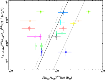
Figure 18: X-ray luminosity in the 0.1-2.4 keV band vs. strong lensing mass within $r_{2500}$ for the S05 subsample (boxes), and weak lensing mass within $r^{wl}_{200}$ for the B06 subsample (circles), respectively. The symbols for the CCCs are solid. The colors have the same meaning as those in Fig. 2. The slope of the fitting is set to 1.73. The grey lines denote the best fit power law for the S05 subsample (dashed) and B06 subsample (solid). The black line denotes the X-ray luminosity–mass relation for the pilot LoCuSS sample at $z\sim 0.2$.

In Fig. 18, we show the luminosity–mass scaling relations using X-ray and lensing masses. We observed the correlation between the strong/weak lensing mass and X-ray luminosity. The scatter using the lensing masses is about 40%, larger than using the X-ray masses ($<20\%$). The large scatter using the strong/weak lensing masses can be due to the combination of (1) the dependence between the X-ray luminosity and X-ray mass since the X-ray luminosity is measured within the scale $2.5r_{500}$ determined by the X-ray approach instead of the scale $r_{200}^{\rm wl}$ determined by the lensing approach, (2) the small size of the sample, (3) the possible additional uncertainties in the X-ray and lensing mass estimates due to the multi-component DM halo, (4) the use of a definition of the global X-ray luminosity such as to reduce the scatter in the X-ray scaling relations, and perhaps (5) the physics for the individual clusters such as central AGNs.

We went through the radio archive, and found that there is potentially one central AGN in each cluster for the LoCuSS sample. There is an evidence of the link between their AGN activities and the scatter of the scaling relation. Abell 1763 shows one twin-jet radio source in the center (e.g. Hardcastle & Sakelliou 2004), and one twin-lobe radio source $\sim 5^{\prime}$ off-center together with an extended low surface brightness X-ray feature. The archive SDSS spectrum shows that the cD galaxy of Abell 1835 is a LINER. As 2 clusters with the most significant indication of AGN activities in the sample, Abell 1763 and Abell 1835 coincidentally introduce the most pronounced scatter in the $L$–$M$ scaling relations using both strong lensing and weak lensing masses.

7 Summary and conclusions

We performed a systematic analysis to measure the X-ray quantities based on XMM-Newton observations for the pilot LoCuSS sample, a flux-limited morphology-unbiased sample at $z\sim 0.2$ consisting of 12 X-ray luminous galaxy clusters. We investigated various X-ray properties, the scaling relations and their scatter, and compared the X-ray and gravitational lensing masses for this sample. We summarize the main conclusions as follows.

(i) Self-similarity of the scaled profiles of the X-ray properties

An almost self-similar behavior of the scaled profiles of X-ray properties, such as temperature, surface brightness, cooling time, entropy, gravitational mass and gas mass, has been found for radii above 0.2 $r_{500}$ for the sample.

• Based on XMM-Newton observations, we obtained an average temperature profile of the sample with a plateau at 0.2–0.5 $r_{500}$ and a drop to 80% of the maximum temperature at $0.5r_{500}$ with 20% scatter. For the 4 CCCs, we observed cool gas showing lower temperatures than 70% of the maximum temperatures in the cluster cores. In the $r<0.2r_{500}$ region, the average temperature profile for the whole sample gives $T(r)\propto r^{0.21\pm 0.04}$, and for the CCC subsample $T(r)\propto r^{0.38\pm 0.04}$, respectively. In the outskirts ($0.2r_{500}<r<r_{500}$), it gives $T(r)\propto r^{-0.36\pm 0.18}$ for the whole sample, without an evident difference between the CCCs and non-CCCs at 1$\sigma$ significance level. The averaged temperature profile for the pilot LoCuSS sample at $z\sim 0.2$ is consistent with the nearby and more distant cluster samples within the observational dispersion

• We determined the XMM-Newton surface brightness profiles up to at least $r_{500}$. The surface brightness profiles of the non-CCCs show flat cores populating a broad range of values up to 0.2 $r_{500}$. For the CCCs, the cluster cores are resolved with current XMM-Newton data. The surface brightness profiles are quite self-similar at $R>0.2r_{500}$ for the sample.

• The scaled cooling time profiles show an almost self-similar behavior above $0.2r_{500}$. The best fit power law above $0.2r_{500}$ gives $t_{\rm c}(r)\propto r^{1.61\pm 0.01}$ for the whole sample, $t_{\rm c}(r)\propto r^{1.70\pm 0.01}$ for the 4 CCCs, and $t_{\rm c}(r)\propto r^{1.54\pm 0.01}$ for the 8 non-CCCs.

• We found an empirical scaling, $S_{0.2r_{500}}\propto T^{0.81\pm 0.19}$. The $S$–$T$ relation for this sample agrees with the REFLEX-DXL sample and the sample in Pratt et al. (2006). After the redshift evolution correction, the entropy profiles for the pilot LoCuSS sample agree with the nearby clusters in Ponman et al. (2003) and Pratt et al. (2006) and the more distant clusters in Zhang et al. (2006) within the observational dispersion. The entropy profiles at $r>0.2r_{500}$ for the whole sample give $S(r)\propto r^{1.01\pm 0.04}$. The non-CCCs show a combined entropy profile of $S(r)\propto r^{0.97\pm 0.05}$. The entropy profiles for the 4 CCCs give, $S(r)\propto r^{1.10\pm 0.05}$, consistent with the spherical accretion shock model prediction.

(ii) X-ray scaling relations

• The scaling relations are sensitive to the exclusion of CCCs when the X-ray luminosity and temperature are measured including the cluster cores. The cluster cores ($<0.2r_{500}$) contribute up to 70% of the bolometric X-ray luminosity. Using the X-ray luminosity corrected for the cool core and temperature excluding the cool core, one not only minimizes the scatter in the scaling relations but also obtains an agreement better than 10% between the normalization for the CCCs and non-CCCs.

• For the pilot LoCuSS sample the mass scatter is less than 20% in the mass observable scaling relations. The X-ray scaling relations show no evident evolution comparing the pilot LoCuSS sample to the nearby and more distant samples within the observational dispersion after the redshift evolution correction. This fits the general opinion (e.g. Maughan et al. 2003; Arnaud 2005; Arnaud et al. 2005; Vikhlinin et al. 2006a; Zhang et al. 2006) that the evolution of galaxy clusters up to $z\sim 1$ is well described by a self-similar model for massive clusters. With the current observations, the X-ray quantities such as temperature and luminosity can be used as reliable indicators of the cluster mass within 20% scatter.

(iii) Mass calibration and the luminosity–mass relation

The discrepancies remain between the X-ray measured cluster masses and the gravitational lensing masses. This can be due to a combination of the measurement uncertainties and the physics in the individual clusters. The scatter in the strong lensing to X-ray mass ratios and weak lensing to X-ray mass ratios, respectively, is similar. We observed the correlation between the X-ray luminosity and lensing mass. The scatter using the gravitational lensing masses is significant ($\sim 40$%). This can be either due to the unknown physics or due to that the sample is too small. A large X-ray selected sample with high quality X-ray and gravitational lensing observations should shed light on it.

Table 1: Primary parameters. Column (1): cluster name; Col. (2): optical redshift (e.g. Smith et al. 2005; Bardeau et al. 2006); Cols. (3,4): sky coordinates in epoch J2000 of the cluster center; Col. (5): hydrogen column density (Dickey & Lockman 1990); Col. (6): truncation radius corresponding to a $S/N$ of 3 of the observational surface brightness profile; Cols. (7–9): bolometric luminosity including the $<0.2r_{500}$ region, excluding the $<0.2r_{500}$ region, and corrected for the $<0.2r_{500}$ region, respectively.

Name	$z_{\rm opt}$	X-ray centroid		$N_{\rm H}$	$r_{\rm t}$	$L_{\rm bol}^{\rm incc}$	$L_{\rm bol}^{\rm excc}$	$L_{\rm bol}^{\rm corr}$
		R.A.	delc.	$10^{22}$ cm-2	arcmin	$10^{45}$erg/s	$10^{45}$erg/s	$10^{45}$erg/s
Abell 68	0.255	00   37   06.159	$+09$  09   28.72	0.0493	6.1	$1.17\pm 0.10$	$0.63\pm 0.07$	$0.89\pm 0.10$
Abell 209	0.209	01   31   52.607	$-13$  36   35.50	0.0164	7.4	$1.25\pm 0.10$	$0.80\pm 0.07$	$1.04\pm 0.10$
Abell 267	0.230	01   52   42.021	$+01$  00   41.17	0.0280	5.3	$0.75\pm 0.07$	$0.35\pm 0.04$	$0.51\pm 0.07$
Abell 383	0.187	02   48   03.340	$-03$  31   43.55	0.0392	7.7	$0.76\pm 0.05$	$0.25\pm 0.04$	$0.34\pm 0.05$
Abell 773	0.217	09   17   52.935	$+51$  43   19.41	0.0144	7.7	$2.06\pm 0.15$	$1.05\pm 0.11$	$1.50\pm 0.15$
Abell 963	0.206	10   17   03.178	$+39$  02   56.53	0.0140	6.1	$1.16\pm 0.09$	$0.56\pm 0.07$	$0.75\pm 0.09$
Abell 1689	0.184	13   11   29.330	$-01$  20   26.66	0.0182	8.0	$2.94\pm 0.10$	$0.96\pm 0.06$	$1.49\pm 0.10$
Abell 1763	0.228	13   35   18.115	$+41$  00   03.89	0.0936	7.5	$1.75\pm 0.15$	$1.21\pm 0.12$	$1.50\pm 0.15$
Abell 1835	0.253	14   01   01.865	$+02$  52   35.48	0.0232	7.0	$5.18\pm 0.17$	$1.56\pm 0.10$	$2.29\pm 0.17$
Abell 2218	0.176	16   35   53.775	$+66$  12   32.43	0.0324	7.7	$1.15\pm 0.08$	$0.70\pm 0.06$	$0.94\pm 0.08$
Abell 2219	0.226	16   40   19.900	$+46$   42   41.00	0.0178	—	—	—	—
Abell 2390	0.233	21   53   37.115	$+17$  41   46.41	0.0680	7.7	$3.90\pm 0.26$	$1.86\pm 0.17$	$2.54\pm 0.26$
Abell 2667	0.230	23   51   39.218	$-26$  05   03.49	0.0165	7.6	$2.10\pm 0.12$	$0.81\pm 0.08$	$1.11\pm 0.12$

The XMM-Newton observations of Abell 2219 are flared.

Table 2: Deduced properties of all 13 galaxy clusters. Column (1): cluster name; Col. (2): electron number density of the inner most radial bin; Col. (3): entropy at $0.2r_{500}$; Col. (4): inner most radial bin of the surface brightness profile; Col. (5): cooling time measured at $r_{\rm cen}$; Col. (6): cooling radius; Col. (7): $r_{500}$; Cols. (8–10): gas mass, total mass and gas mass fraction at $r_{500}$.

Name	$n_{e0}$	$S_{0.2r_{500}}$	$r_{\rm cen}$	$t_{\rm c}$	$r_{\rm cool}$	$r_{500}$	$M_{\rm gas,500}$	$M_{500}$	$f_{\rm gas,500}$
$10^{-3}$ cm-3		keV cm2	kpc	Gyr	$r_{500}$	Mpc	$10^{14}M_{\odot}$	$10^{14}M_{\odot}$
Abell 68	$6.4\pm 0.3$	$487\pm 35$	$3.55$	$6.6\pm 0.2$	$0.10$	$1.21$	$0.68\pm 0.07$	$6.51\pm 1.93$	$0.105\pm 0.060$
Abell 209	$5.7\pm 0.2$	$370\pm 26$	$3.74$	$6.4\pm 0.3$	$0.14$	$1.15$	$0.77\pm 0.08$	$5.33\pm 1.71$	$0.146\pm 0.089$
Abell 267	$7.4\pm 0.4$	$365\pm 33$	$3.29$	$4.9\pm 0.4$	$0.15$	$1.06$	$0.47\pm 0.04$	$4.29\pm 1.30$	$0.109\pm 0.060$
Abell 383	$54.6\pm 1.5$	$303\pm 14$	$1.98$	$0.5\pm 0.2$	$0.16$	$0.98$	$0.33\pm 0.04$	$3.17\pm 0.94$	$0.104\pm 0.061$
Abell 773	$7.4\pm 0.4$	$434\pm 41$	$3.15$	$5.7\pm 0.5$	$0.14$	$1.33$	$1.05\pm 0.12$	$8.30\pm 2.45$	$0.126\pm 0.070$
Abell 963	$14.3\pm 0.8$	$393\pm 18$	$2.14$	$2.6\pm 0.2$	$0.14$	$1.14$	$0.62\pm 0.07$	$5.19\pm 1.52$	$0.120\pm 0.066$
Abell 1689	$30.1\pm 0.9$	$505\pm 25$	$1.95$	$1.5\pm 0.2$	$0.13$	$1.44$	$1.05\pm 0.14$	$10.26\pm 2.96$	$0.102\pm 0.060$
Abell 1763	$6.5\pm 0.3$	$402\pm 47$	$4.00$	$6.1\pm 0.5$	$0.13$	$1.12$	$0.88\pm 0.08$	$4.96\pm 1.46$	$0.178\pm 0.094$
Abell 1835	$60.8\pm 1.2$	$334\pm 20$	$2.50$	$0.6\pm 0.3$	$0.19$	$1.22$	$1.14\pm 0.11$	$6.62\pm 1.94$	$0.172\pm 0.092$
Abell 2218	$5.8\pm 0.2$	$444\pm 51$	$3.26$	$8.0\pm 0.5$	$0.12$	$1.07$	$0.62\pm 0.06$	$4.18\pm 1.27$	$0.147\pm 0.085$
Abell 2390	$40.1\pm 1.6$	$486\pm 34$	$2.31$	$0.9\pm 0.3$	$0.14$	$1.29$	$1.21\pm 0.16$	$7.67\pm 2.28$	$0.158\pm 0.095$
Abell 2667	$40.7\pm 1.4$	$399\pm 27$	$2.33$	$0.8\pm 0.3$	$0.15$	$1.19$	$0.77\pm 0.09$	$6.02\pm 1.74$	$0.128\pm 0.073$
Mean	—	—	—	—	—	—	—	—	$0.13\pm 0.01$

Table 3: Generalized NFW model fit. Column (1): cluster name; Cols. (2,3): characteristic density and scale of the halo of the generalized NFW fit; Col. (4): slope parameter of the generalized NFW fit.

Name	$\rho_{\rm s}$	$r_{\rm s}$	$\alpha$
	$10^{14}M_{\odot}$ Mpc-3	Mpc
Abell 68	$82\pm 3$	$0.203\pm 0.005$	$0.000\pm 0.100$
Abell 209	$38\pm 5$	$0.289\pm 0.018$	$0.000\pm 0.063$
Abell 267	$82\pm 5$	$0.184\pm 0.008$	$0.000\pm 0.100$
Abell 383	$108\pm 15$	$0.127\pm 0.008$	$0.518\pm 0.044$
Abell 773	$53\pm 2$	$0.262\pm 0.006$	$0.000\pm 0.100$
Abell 963	$173\pm 33$	$0.126\pm 0.010$	$0.000\pm 0.090$
Abell 1689	$64\pm 14$	$0.220\pm 0.021$	$0.608\pm 0.070$
Abell 1763	$69\pm 6$	$0.187\pm 0.010$	$0.000\pm 1.000$
Abell 1835	$275\pm 11$	$0.117\pm 0.002$	$0.000\pm 0.100$
Abell 2218	$123\pm 4$	$0.149\pm 0.003$	$0.000\pm 1.000$
Abell 2390	$128\pm 20$	$0.168\pm 0.011$	$0.324\pm 0.055$
Abell 2667	$165\pm 14$	$0.142\pm 0.005$	$0.037\pm 0.035$

Table 4: Cluster global temperatures and metallicities. Column (1): cluster name; Col. (2,3): volume averaged radial temperature profile of 0.1–0.5 $r_{500}$ and 0.2–0.5 $r_{500}$, respectively; Col. (4-9): spectral measured temperatures and metallicities of the annuli of $R<2/3r_{\rm t}$, $0.1r_{500}<R<0.5r_{500}$ and $0.2r_{500}<R<0.5r_{500}$, respectively.

Name	$T_{0.1-0.5r_{500}}$	$T_{0.2-0.5r_{500}}$	$T^{\rm spec}_{<2/3r_{\rm t}}$	$T^{\rm spec}_{0.1-0.5r_{500}}$	$T^{\rm spec}_{0.2-0.5r_{500}}$	$Z_{<2/3r_{\rm t}}$	$Z_{0.1-0.5r_{500}}$	$Z_{0.2-0.5r_{500}}$
	keV	keV	keV	keV	keV	$Z_{\odot}$	$Z_{\odot}$	$Z_{\odot}$
Abell 68	$8.2\pm 0.3$	$7.7\pm 0.3$	$7.9\pm 0.3$	$7.7\pm 0.3$	$7.3\pm 0.3$	$0.17\pm 0.05$	$0.15\pm 0.04$	$0.12\pm 0.05$
Abell 209	$6.4\pm 0.2$	$7.1\pm 0.3$	$6.9\pm 0.2$	$7.0\pm 0.2$	$7.1\pm 0.3$	$0.28\pm 0.04$	$0.23\pm 0.03$	$0.22\pm 0.04$
Abell 267	$6.1\pm 0.2$	$6.5\pm 0.4$	$6.1\pm 0.2$	$6.1\pm 0.2$	$6.2\pm 0.4$	$0.23\pm 0.05$	$0.23\pm 0.05$	$0.25\pm 0.08$
Abell 383	$4.6\pm 0.1$	$5.3\pm 0.2$	$4.5\pm 0.1$	$4.7\pm 0.1$	$4.7\pm 0.2$	$0.44\pm 0.04$	$0.29\pm 0.04$	$0.18\pm 0.06$
Abell 773	$7.8\pm 0.3$	$8.1\pm 0.4$	$7.9\pm 0.2$	$7.8\pm 0.3$	$8.3\pm 0.4$	$0.30\pm 0.03$	$0.26\pm 0.04$	$0.30\pm 0.06$
Abell 963	$6.5\pm 0.2$	$6.3\pm 0.2$	$6.4\pm 0.2$	$6.5\pm 0.2$	$6.5\pm 0.2$	$0.31\pm 0.04$	$0.30\pm 0.03$	$0.28\pm 0.05$
Abell 1689	$9.0\pm 0.2$	$8.4\pm 0.2$	$9.0\pm 0.1$	$9.0\pm 0.2$	$8.5\pm 0.2$	$0.26\pm 0.02$	$0.24\pm 0.02$	$0.26\pm 0.04$
Abell 1763	$7.1\pm 0.2$	$6.3\pm 0.3$	$6.3\pm 0.2$	$6.1\pm 0.2$	$5.8\pm 0.3$	$0.27\pm 0.05$	$0.23\pm 0.04$	$0.20\pm 0.05$
Abell 1835	$7.6\pm 0.2$	$8.0\pm 0.3$	$7.2\pm 0.1$	$8.1\pm 0.2$	$8.4\pm 0.3$	$0.29\pm 0.02$	$0.25\pm 0.02$	$0.23\pm 0.04$
Abell 2218	$8.0\pm 0.2$	$7.4\pm 0.3$	$6.9\pm 0.2$	$6.9\pm 0.2$	$6.6\pm 0.3$	$0.25\pm 0.04$	$0.18\pm 0.21$	$0.21\pm 0.04$
Abell 2390	$9.7\pm 0.4$	$10.6\pm 0.6$	$10.1\pm 0.3$	$10.6\pm 0.4$	$11.6\pm 0.6$	$0.35\pm 0.04$	$0.28\pm 0.04$	$0.24\pm 0.06$
Abell 2667	$7.0\pm 0.2$	$7.3\pm 0.3$	$6.6\pm 0.1$	$7.2\pm 0.2$	$7.0\pm 0.3$	$0.34\pm 0.03$	$0.30\pm 0.03$	$0.29\pm 0.04$

Table 5: Power law, $Y=Y_{0}\;X^{\gamma}$, parameterized X-ray scaling relations.

$X$	$Y$	$Y_{0}$	$\gamma$	Scatter		Sample
				$X$	$Y$
$\frac{T_{0.2-0.5r_{500}}}{\rm keV}$	$\frac{S_{0.2r_{500}}}{\rm keV\;cm^{2}}\;E(z)^{4/3}\;\left(\frac{\Delta_{c,z}}{\Delta_{c,0}}\right)^{2/3}$	$10^{2.08\pm 0.26}$	$0.90\pm 0.30$	—	—	REFLEX-DXL
		$10^{2.00\pm 0.16}$	$0.81\pm 0.19$	—	—	pilot LoCuSS sample
		$10^{1.96\pm 0.22}$	$0.89\pm 0.25$	—	—	non-CCC subsample
		$10^{2.04\pm 0.18}$	$0.71\pm 0.21$	—	—	CCC subsample
$\frac{r}{r_{500}}$	$\frac{S}{\rm keV\;cm^{2}}\;E(z)^{4/3}\;\left(\frac{\Delta_{c,z}}{\Delta_{c,0}}\right)^{2/3}\left(\frac{T_{0.2-0.5r_{500}}}{10keV}\right)^{-0.65}$	$10^{3.52\pm 0.03}$	$1.00\pm 0.07$	—	—	REFLEX-DXL
		$10^{3.50\pm 0.02}$	$1.01\pm 0.04$	—	—	pilot LoCuSS sample
		$10^{3.49\pm 0.02}$	$0.97\pm 0.05$	—	—	non-CCC subsample
		$10^{3.52\pm 0.02}$	$1.10\pm 0.05$	—	—	CCC subsample
$\frac{T_{0.2-0.5r_{500}}}{\rm keV}$	$\frac{M_{500}}{M_{\odot}}\;E(z)\;\left(\frac{\Delta_{c,z}}{\Delta_{c,0}}\right)^{0.5}$	$10^{13.69\pm 0.03}h_{70}^{-1}$	1.5 (fixed)	0.05	0.15	pilot LoCuSS sample
		$10^{13.72\pm 0.04}h_{70}^{-1}$	1.5 (fixed)	0.05	0.20	non-CCC subsample
		$10^{13.91\pm 0.38}h_{70}^{-1}$	$1.24\pm 0.44$	0.06	0.15	pilot LoCuSS sample
		$10^{13.41\pm 0.53}h_{70}^{-1}$	$1.87\pm 0.63$	0.07	0.19	non-CCC subsample
$\frac{T_{0.2-0.5r_{500}}}{\rm keV}$	$\frac{M_{\rm gas,500}}{M_{\odot}}\;E(z)\;\left(\frac{\Delta_{c,z}}{\Delta_{c,0}}\right)^{0.5}$	$10^{12.54\pm 0.04}h_{70}^{-1}$	1.8 (fixed)	0.06	0.10	pilot LoCuSS sample
		$10^{12.54\pm 0.05}h_{70}^{-1}$	1.8 (fixed)	0.06	0.11	non-CCC subsample
		$10^{11.72\pm 0.70}h_{70}^{-1}$	$2.76\pm 0.81$	0.05	0.13	pilot LoCuSS sample
		$10^{11.65\pm 0.98}h_{70}^{-1}$	$2.86\pm 1.17$	0.05	0.13	non-CCC subsample
$\frac{T_{0.2-0.5r_{500}}}{\rm keV}$	$\frac{L_{\rm 0.1-2.4keV}^{\rm corr}}{\rm erg\;s^{-1}}\;E(z)^{-1}\;\left(\frac{\Delta_{c,z}}{\Delta_{c,0}}\right)^{-0.5}$	$10^{42.31\pm 0.04}h_{70}^{-1}$	2.60 (fixed)	0.05	0.12	pilot LoCuSS sample
		$10^{42.30\pm 0.05}h_{70}^{-1}$	2.60 (fixed)	0.05	0.13	non-CCC subsample
		$10^{41.87\pm 0.71}h_{70}^{-1}$	$3.11\pm 0.82$	0.04	0.13	pilot LoCuSS sample
		$10^{42.17\pm 0.86}h_{70}^{-1}$	$2.76\pm 1.01$	0.05	0.14	non-CCC subsample
$\frac{T_{0.2-0.5r_{500}}}{\rm keV}$	$\frac{L_{\rm bol}^{\rm corr}}{\rm erg\;s^{-1}}\;E(z)^{-1}\;\left(\frac{\Delta_{c,z}}{\Delta_{c,0}}\right)^{-0.5}$	$10^{42.39\pm 0.04}h_{70}^{-1}$	2.98 (fixed)	0.04	0.12	pilot LoCuSS sample
		$10^{42.38\pm 0.05}h_{70}^{-1}$	2.98 (fixed)	0.05	0.13	non-CCC subsample
		$10^{41.84\pm 0.70}h_{70}^{-1}$	$3.62\pm 0.80$	0.04	0.13	pilot LoCuSS sample
		$10^{41.95\pm 0.90}h_{70}^{-1}$	$3.49\pm 1.06$	0.04	0.14	non-CCC subsample
$\frac{M_{500}}{M_{\odot}}\;E(z)\;\left(\frac{\Delta_{c,z}}{\Delta_{c,0}}\right)^{0.5}$	$\frac{L_{\rm 0.1-2.4keV}^{\rm corr}}{\rm erg\;s^{-1}}\;E(z)^{-1}\;\left(\frac{\Delta_{c,z}}{\Delta_{c,0}}\right)^{-0.5}$	$10^{18.65\pm 0.04}h_{70}^{-1}$	1.73 (fixed)	0.14	0.11	pilot LoCuSS sample
		$10^{18.61\pm 0.04}h_{70}^{-1}$	1.73 (fixed)	0.19	0.12	non-CCC subsample
		$10^{18.12\pm 4.74}h_{70}^{-1}$	$1.77\pm 0.32$	0.14	0.11	pilot LoCuSS sample
		$10^{22.85\pm 3.51}h_{70}^{-1}$	$1.45\pm 0.23$	0.19	0.12	non-CCC subsample
$\frac{M_{500}}{M_{\odot}}\;E(z)\;\left(\frac{\Delta_{c,z}}{\Delta_{c,0}}\right)^{0.5}$	$\frac{L_{\rm bol}^{\rm corr}}{\rm erg\;s^{-1}}\;E(z)^{-1}\;\left(\frac{\Delta_{c,z}}{\Delta_{c,0}}\right)^{-0.5}$	$10^{15.16\pm 0.04}h_{70}^{-1}$	1.99 (fixed)	0.14	0.12	pilot LoCuSS sample
		$10^{15.11\pm 0.04}h_{70}^{-1}$	1.99 (fixed)	0.19	0.13	non-CCC subsample
		$10^{14.16\pm 5.39}h_{70}^{-1}$	$2.06\pm 0.36$	0.14	0.12	pilot LoCuSS sample
		$10^{19.88\pm 3.19}h_{70}^{-1}$	$1.67\pm 0.21$	0.19	0.13	non-CCC subsample

Figure 1: De-projected temperature profiles (upper panels), surface brightness profiles (middle panels) and mass profiles (lower panels). The temperature profiles are approximated by the parameterization $T(r)=T_{3}\exp[-(r-T_{1})^{2}/T_{2}]+T_{6}(1+r^{2}/T_{4}^{2})^{-T_{5}}+T_{7}$ crossing all the data points (solid). The vertical line denotes $0.1r_{500}$. The surface brightness profiles are parameterized by double-$\beta$ model. The observed mass profiles are fitted by generalized NFW model.

Appendix A XMM-Newton observational information

Table 6: Observational information of the XMM-Newton data.

Name	Date	Id	Filter	Frame		Net exposure (ks)
				MOS	pn	MOS1	MOS2	pn
Abell 68	2006-03-14	0084230201	Medium	FF	EFF	24.94	23.81	18.15
Abell 209	2001-01-15	0084230301	Medium	FF	EFF	17.33	16.09	12.80
Abell 267	2002-01-02	0084230401	Medium	FF	EFF	16.06	15.74	10.96
Abell 383	2002-08-17	0084230501	Medium	FF	EFF	28.07	28.05	21.50
Abell 773	2001-04-26	0084230601	Medium	FF	EFF	13.01	14.68	15.90
Abell 963	2001-11-02	0084230701	Medium	FF	EFF	23.82	24.69	17.92
Abell 1689	2001-12-24	0093030101	Thin	FF	EFF	33.67	33.34	29.24
Abell 1763	2002-12-13	0084230901	Medium	FF	EFF	12.32	12.01	9.34
Abell 1835	2000-06-28	0098010101	Thin	FF	FF	—	25.27	24.73
Abell 2218	2002-09-28	0112980101	Thin	FF	EFF	16.69	16.91	13.79
Abell 2219	2002-06-14	0112231801	Medium	FF	EFF	—	—	—
	2002-06-24	0112231901	Medium	FF	EFF	—	—	—
Abell 2390	2001-06-19	0111270101	Thin	FF	FF	10.27	10.03	8.85
Abell 2667	2003-06-21	0148990101	Medium	FF	FF	22.21	22.87	14.10

The MOS1 data of Abell 1835 are in window mode, which cannot be used for this work. The XMM-Newton observations of Abell 2219 are flared.

Appendix B Individual cluster profiles

Figure 19: See the caption in Fig. 1.

Figure 20: See the caption in Fig. 1.

Figure 21: See the caption in Fig. 1.

Figure 22: See the caption in Fig. 1.

Figure 23: See the caption in Fig. 1.