Polarisation studies of the prompt gamma-ray emission from GRB 041219a using the Spectrometer aboard INTEGRAL

Linear polarisation in gamma-ray burst prompt emission is an important diagnostic with the potential to significantly constrain models. The spectrometer aboard INTEGRAL, SPI, has the capability to detect the signature of polarised emission from a bright $\gamma$–ray source. GRB 041219a is the most intense burst localised by INTEGRAL with a fluence of 5.7 $\times 10^{-4}$ ergs cm^-2 over the energy range 20 keV–8 MeV and is an ideal candidate for such a study. Polarisation can be measured using multiple events scattered into adjacent detectors because the Compton scatter angle depends on the polarisation of the incoming photon. A search for linear polarisation in the most intense pulse of duration 66 seconds and in the brightest 12 seconds of GRB 041219a was performed in the 100–350 keV, 100–500 keV and 100 keV–1 MeV energy ranges. It was possible to divide the events into six directions in the energy ranges of 100–350 keV and 100–500 keV using the kinematics of the Compton scatter interactions. The multiple event data from the spectrometer was analysed and compared with the predicted instrument response obtained from Monte–Carlo simulations using the GEANT 4 INTEGRAL mass model. The $\chi^{2}$ distribution between the real and simulated data as a function of the percentage polarisation and polarisation angle was calculated for all three energy ranges. The degree and angle of polarisation were obtained from the best–fit value of $\chi^{2}$. A weak signal consistent with polarisation was found throughout the analyses. The degree of linear polarisation in the brightest pulse of duration 66 s was found to be $63^{+31}_{-30}$% at an angle of $70^{+14}_{-11}$ degrees in the 100–350 keV energy range. The degree of polarisation was also constrained in the brightest 12 s of the GRB and a polarisation fraction of $96^{+39}_{-40}$% at an angle of $60^{+12}_{-14}$ degrees was determined over the same energy range. However, despite extensive analysis and simulations, a systematic effect that could mimic the weak polarisation signal could not be definitively excluded. Our results over several energy ranges and time intervals are consistent with a polarisation signal of about 60% but at a low level of significance ($\sim 2\sigma$). The polarisation results are compared with predictions from the synchrotron and Compton drag processes. The spectrum of this GRB can also be well fit by a combined black body and power law model which could arise from a combination of the Compton and synchrotron processes, with different degrees of polarisation. We therefore conclude that the procedure described here demonstrates the effectiveness of using SPI as a polarimeter, and is a viable method of measuring polarisation levels in intense gamma–ray bursts.

1 Introduction

Polarisation is a powerful tool for investigating emission processes in long gamma–ray bursts (GRBs). The link between the $\gamma$-ray production mechanism and the degree of linear polarisation can be exploited to constrain models.

Long gamma ray bursts are linked to the collapse of a massive star which forms a rapidly rotating black hole. For a recent review of GRBs, see Mészáros (2006). In addition, a large ordered magnetic field may be induced by the angular momentum of the accretion disk (Zhang & Mészáros, 2004; Piran, 2004). Energetic outflows develop which are beamed perpendicular to the accretion disk and along the black hole’s rotation axis. An observer close to the jet axis will detect a GRB. Polarisation is generally associated with an asymmetry in the way that the material is viewed. The asymmetry can be attributed to a preferential orientation of the magnetic field or to inverse Compton scattering. The polarisation mechanisms are discussed in more detail in §7.

The reported detection of significant polarisation ($\Pi_{s}=80\pm 20\%$ in the energy range 15–2000 keV) in GRB 021206 (Coburn & Boggs, 2003) using the RHESSI spacecraft led to many publications examining the results (Rutledge & Fox, 2004; Wigger et al., 2004; Boggs & Coburn, 2003) and the mechanisms for producing large polarisation (e.g. Shaviv & Dar, 1995; Nakar et al., 2003; Waxman, 2003; Granot, 2003; Lazzati et al., 2004; Dado et al., 2007). The RHESSI results highlighted the importance of correctly evaluating the systematic effects, which may mimic a polarisation signature. A recent novel attempt (Willis et al., 2005) involved analysing the Earth’s albedo flux seen by BATSE for GRB 930131 and GRB 960924, where the lower limits of polarisation were found to be $\Pi_{s}$ $>$ 35% and $\Pi_{s}$ $>$ 50% respectively. These figures can only be considered as lower limits due to systematic effects, including natural anisotropies in the Earth’s albedo flux and possible limitations in the GEANT 4 code at the time the simulation was run.

The dominant mode of interaction for photons in the energy range of a few hundred keV is Compton scattering. Linearly polarised $\gamma$–rays preferentially scatter perpendicular to the incident polarisation vector, resulting in an azimuthal scatter angle distribution (ASAD) which is modulated relative to the distribution for unpolarised photons. The sensitivity of an instrument to polarisation is determined by its effective area to scatter events and the average value of the polarimetric modulation factor, Q, which is the maximum variation in azimuthal scattering probability for polarised photons (Lei et al., 1997). The value of Q is given by

$$Q=\frac{d\sigma_{\bot}-d\sigma_{\parallel}}{d\sigma_{\bot}+d\sigma_{\parallel}}$$ (1)

where d$\sigma_{\bot}$, d$\sigma_{\parallel}$ are the Klein-Nishina differential cross-sections for Compton scattering perpendicular and parallel to the polarisation direction, respectively. Q is a function of incident photon energy, E, and the Compton scatter angle, $\theta$, between the incident and scattered photon directions. For a source of count rate S and fractional polarisation $\Pi_{s}$, the expected ASAD is given by:

$$\frac{\partial S}{\partial\phi}={\left(\frac{S}{2\pi}\right)}{\left[1-Q\Pi_{s}\cos 2(\phi-\eta)\right]}$$ (2)

where $\phi$ is the scattering angle, and $\eta$ is the polarisation angle (Lei et al., 1997). This equation yields a 180$\degr$ modulated curve when fit to polarised data, where $\eta$ represents the minimum angle of the modulated distribution and gives the direction of the polarisation vector.

1.1 SPI as a polarimeter

SPI is not optimised to act as a polarimeter, but because of its detector layout, geometry and thick detector plane, the modulation from a polarised flux can be measured through multiple scatter events in its detectors. Kalemci et al. (2004) found that it is possible to measure polarisation in a moderately bright GRB in the field of view of SPI if the GRB is on–axis. GRB 041219a had a fluence of 5.7 $\times 10^{-4}$ ergs cm^-2 and a peak flux of 1.84 $\times 10^{-5}$ ergs cm^-2 s^-1 (20 keV–8 MeV) at an off–axis angle of 3.2^∘ and is the most intense burst detected by INTEGRAL, so would appear to be an ideal candidate (McBreen et al., 2006). Detailed Monte–Carlo simulations built with the GEANT 4 toolkit can be used to predict the response of SPI to a polarised flux. A comparison of the data and simulations enables a determination of the polarisation strength and angle.

Figure 1: The numbering system used for the Germanium SPI detectors. The 6 directions used in the polarisation analysis are shown along with the y– and z–coordinate axes of the spacecraft. The x–axis is normal to the detector plane.

2 The Spectrometer aboard INTEGRAL

The European Space Agency’s International Gamma-Ray Astrophysics Laboratory, INTEGRAL, was launched on 17 October 2002 (Winkler et al., 2003). It consists of two coded mask $\gamma$–ray instruments, the spectrometer (SPI) and the imager (IBIS). The instruments are coaligned so that data is taken by all instruments in one pointing.

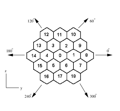
SPI consists of 19 hexagonal germanium (Ge) detectors (Vedrenne et al., 2003), arranged to minimise the volume of the array and the space between each detector (Fig. 1). The detectors cover the energy range 20 keV–8 MeV with an energy resolution of 2.5 keV at 1.3 MeV. Each detector is 6.9 cm in height, with a centre to centre distance of $\sim$ 6 cm between adjacent crystals. A coded mask is located 1.71 m above the detector plane for imaging purposes, giving a 16^∘ corner–to–corner field of view. The sensitivity of SPI ($\sim$ 5 $\times 10^{-6}$ photons cm^-2 s^-1 keV^-1) is limited by the instrumental background, which consists mainly of cosmic rays impinging on the detectors and the secondary particles created by their interaction (Jean et al., 2003; Weidenspointner et al., 2003). The background can be determined by averaging the count rate over a long period of time during the science window, and subtracting this average from the raw count rate. The background is significantly reduced by the presence of an anti–coincidence shield made from BGO crystals surrounding the Ge detectors.

The operating mode of SPI is based on the detection of events from the Ge detectors which are not accompanied by a corresponding detection in the anti–coincidence shield. The events are separated into single events (SE) where a photon deposits energy in one detector, and multiple events (ME) where the photon deposits energy in two or more detectors. All events are processed by the Digital Front End Electronics (DFEE), which provides event timing and classification. SPI operates in photon–by–photon mode, which produces photon packets (80 packets/8 s) containing all of the non–vetoed events and scientific housekeeping packets (5 packets/8 s) including the event counters which are used to generate lightcurves.

Detectors 2 and 17 ceased to function on December 6, 2003, and July 17, 2004 respectively. The failure of these detectors results in a decrease of the effective area of the instrument to about 90% of the original area for SEs. It is reduced to $\sim$ 75% for MEs, because the number of pseudo detectors (i.e. the adjacent detector pairs used to measure multiple events) drops from 84 to 64.

3 Model simulation

The advent of fast computing clusters has made difficult computational tasks such as the prediction of instrument response to polarised flux more feasible. A computer model of the INTEGRAL spacecraft written in the GEANT 4 toolkit (Agostinelli et al., 2003) was used for simulations in this work. This model was developed from the GEANT 3 INTEGRAL Mass–Model (TIMM) (Ferguson et al., 2003) originally used to assess the background recorded by the instruments onboard INTEGRAL. The model contains an accurate representation of the SPI instrument, including the mask and veto elements. The rest of the spacecraft is modelled to a much lower level of detail. Average densities and simplified geometries are used for areas of the spacecraft positioned at larger distances from the detectors since they will not have a large effect on the on–axis gamma–rays.

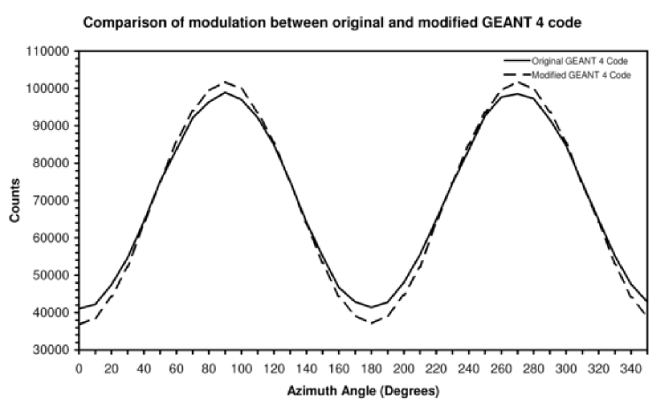
The GEANT 4 toolkit contains all the physics necessary to allow the tracking of photons and particles through a modelled geometry. The software consists of a series of random number generators to calculate the probability of an interaction occurring in a material. As with any program, the simulation is dependent on the coding of the interaction in the software. Mizuno et al. (2005) reported an incorrect implementation of the polarised Compton and Rayleigh scattering processes in the GEANT 4 code. This error caused the azimuthal modulation due to the polarisation to be lower than expected. When the appropriate correction was applied, an increase of $\sim$15% was seen, even in the higher energy regime used in our simulations (Fig. 2).

Figure 2: Simulated modulation due to Compton Scattering in a test geometry. The solid line gives the original GEANT 4 Compton scatter code and the dashed line gives the Compton scatter code using modifications from Mizuno et al. (2005).

Figure 3: The mask elements (yellow) overlaying the detectors (blue), as viewed from the direction of the incoming GRB photons generated from the simulations. Fig. 1 shows the number allocated to each detector.

3.1 Simulating GRB 041219a

Gamma–ray photons were directed into the model geometry from a plane surface in the direction of the GRB, 3.08^∘ from the INTEGRAL x–axis and 63.95^∘ from the INTEGRAL z–axis, simulating the incoming flux from a source at infinity from the same direction relative to the spacecraft as the GRB. The Band model (Band et al., 1993) parameters for the main peak of the burst of duration 66 seconds ($\alpha$ = $-1.50\leavevmode\nobreak\ ^{+0.08}_{-0.06}$, $\beta$ = $-1.95\leavevmode\nobreak\ ^{+0.08}_{-0.21}$, E₀ = 568 ${}^{+310}_{-205}$ keV) were used to create the spectrum (see $\S$4.2). This 66 s interval was selected to maximise the source counts.

For each simulation run, the polarisation angle of the photons was set between 0^∘ and 180^∘ in 10 degree steps, and the polarisation fraction was set to 100%. There was also one run for a beam of unpolarised photons. Only polarisation angles between 0^∘ and 180^∘ were simulated due to the symmetry of the system and the difficulty in separating the scattering directions between the pixels. The effect of the spectral shape on the level of polarisation was simulated, and it was found that the simulated polarisation signal depended very weakly on the spectral parameters. The secondary photons produced by the multiple events scatter more in the forward direction at higher energies, causing the azimuthal modulation to drop slightly. At lower energies the multiple events are less likely to occur due to the photoelectric effect dominating the scatter processes.

The simulations produced a list of all the interactions that occurred in the sensitive volumes of the model (Ge detectors and BGO shield). These data were then converted into an event list, for comparison to the real SPI data. Initially the interactions were summed, so that the energy deposits correspond to the total energy deposited for an event in each of the sensitive volumes. These deposits were then filtered according to the energy thresholds of the detectors ($\sim$20 keV) and veto ($\sim$80 keV). After subtracting the vetoed events, the event list was separated into single events (where the photon is detected in one pixel) and multiple events (where the photon is detected in multiple pixels). This process produced the final list of events to analyse and compare to the real data. The unpolarised simulation data was combined with the polarised simulation data, allowing the percentage of polarisation to be changed for each angle.

4 SPI Data Analysis

GRB 041219a was detected by IBAS at 01:42:18 UTC on December 19^th 2004 (Götz et al., 2004) at a location of 00h 24m 25.8s, +62^° 50^′ 05.6^′′ close to the axis of the detector.

4.1 Temporal Analysis

Figure 4: Background-subtracted single event lightcurve of GRB 041219a, summed over all SPI detectors in the energy range 20 keV–8 MeV. The vertical solid lines mark the start and end of the 66 second emission phase (T₀ = 261 s to T₀ = 327 s). The vertical dashed lines mark the start and end of the brightest 12 seconds of the burst (T₀ = 276 s to T₀ = 288 s). T₀ is the IBAS trigger time (01:42:18 UTC).

GRB 041219a consisted of an initial precursor–type pulse, followed by a quiescent period lasting approximately 200 s, before the main emission beginning at $\sim$ 250 s post–trigger. An image of the coded mask as seen from the direction of the incoming GRB photons was obtained from the simulations (Fig. 3). The background–subtracted single event lightcurve summed over all of the detectors was generated and is shown in Fig. 4. The mask almost completely obscured three of the detectors (12, 3, 0), and partially obscured five more (4–6, 8, 13) (Fig. 6). Also, detectors 2 and 17 are no longer functioning (and were not included in the analysis). However, the GRB can be clearly recognised in at least nine of the SE lightcurves in Fig. 6.

Figure 5: (a) Band model fit to GRB041219a and residuals for the 66 s emission phase (Fig. 4). (b) $\nu$F_ν spectrum of GRB 041219a. The Band model parameters are $\alpha=-1.50$, $\beta=-1.95$ and E₀ = $568$ keV.

4.2 Spectral Analysis

The spectrum of GRB 041219a was extracted using specific GRB tools from the Online Software Analysis (Diehl et al., 2003; Skinner & Connell, 2003) version 5.0 available from the INTEGRAL Science Data Centre. GRB 041219a is the brightest burst localised by INTEGRAL with a peak flux of 43 ph cm^-2 s^-1 (20 keV–8 MeV). The spectrum of the burst and sub-intervals were well fit by the Band model (Band et al., 1993), although the parameters of the spectrum evolved during the burst. A detailed discussion of the spectral and temporal behaviour of this burst is available in McBreen et al. (2006). The most intense emission pulse of duration 66 s (indicated by the solid lines in Fig. 4) was selected for polarisation analysis. The photon indices, $\alpha$ and $\beta$, for the emission phase used to calculate the polarisation were $-1.50\leavevmode\nobreak\ ^{+0.08}_{-0.06}$ and $-1.95\leavevmode\nobreak\ ^{+0.08}_{-0.21}$ respectively. The break energy E₀ was $568\leavevmode\nobreak\ ^{+310}_{-205}$ keV. The spectra are shown in Fig. 5. The peak energy, E_peak, is given by $(2+\alpha)\times\,E_{\rm 0}$ and the value of E_peak in the interval of the main emission phase is $284\leavevmode\nobreak\ ^{+310}_{-74}$ keV. In addition, the polarisation analysis was performed for the brightest 12 s of the 66 s interval to determine the polarisation over the duration of this intense pulse.

Figure 6: The layout of the 19 detectors of SPI with single event lightcurves of GRB 041219a showing the variation in count rate per detector. The horizontal and vertical axes give the time and count rate in each detector respectively. The detector number is indicated in the corner of each lightcurve. Detectors 2 and 17 are not in operation. The detectors with high count rate were unobscured or partially obscured by the mask (Fig. 3).

It is interesting to note that the spectrum of GRB 041219a was equally well fit by a combination of a black body and power law model (McBreen et al., 2006). Fan et al. (2005) also found that the early optical and infrared emission from GRB 041219a can be modelled as the superposition of a reverse and a forward shock component. The ejecta are magnetised to a small extent, which may be due to magnetic field generation during the internal shock phase. Fan et al. (2005) predicted that the internal shock emission was very likely to be linearly polarised.

5 Polarisation Analysis

There is no positional resolution within the SPI detectors and so it is not possible to determine the exact position of the interaction within an individual detector. Centre–to–centre interactions are assumed for multiple events. According to the simulations, this will introduce an uncertainty on each angle of $\sim$29$\degr$. Below 511 keV, the incoming photons predominantly Compton scatter from the detector with the lower energy deposit to the higher one (Kalemci et al., 2004). Thus 6 directions of scatter can be distinguished. For higher energies, the order of energy deposition does not distinguish between anti–parallel directions and the number of directions is limited to 3. To enable a larger energy range from 100 keV–1 MeV to be investigated, the analysis was also performed in 3 directions.

5.1 Method

The analysis procedure was carried out, starting with the raw data from SPI, as follows:

1. All interactions between detectors (double events) during the defined time intervals were selected.

2. Only double events that occurred in adjacent detectors were accepted.

3. The list of events was calibrated (using the spi_gain_corr tool from OSA 5.0) to convert the original channel number to energy in keV.

4. All interactions with less than 30 keV deposited per detector were rejected. Relatively few photons above 100 keV will lose $<$ 30 keV in Compton scatter interactions.

5. Coincident pairs whose combined energies lie in the 100–350 keV range were selected. Up to 511 keV, incoming photons predominantly scatter from the detector with the lower energy deposit to the higher one allowing 6 separate directions to be determined.

6. The scatter pairs were divided into 6 different directions (0–300 degrees) and the total number of events in each direction were determined (Fig. 1).

7. Background events (using the same selection process) were selected from intervals in the same science window before the GRB occurred (Table 1), since the emission continued up to the end of the science window. The scaled background was then subtracted from the multiple event list. The set of 19 detectors was also divided into 4 quadrants and the total background was calculated separately for each quadrant to ensure that there were no biases in any specific direction or systematic effects.

Table 1: Time intervals used for the background determination in 6 directions.

Observation	Start Time (UTC)	End Time (UTC)
Background 1	01:30:00	01:31:06
Background 2	01:35:00	01:36:06
Background 3	01:36:30	01:37:36
Background 4	01:38:00	01:39:06
Total (sec)		264

The analysis was carried out for 6 directions in the energy ranges 100–350 keV and 100–500 keV and over two separate time intervals (Fig. 4) as described above. The analysis was also performed for 3 directions in the 100–350 keV, 100–500 keV and 100 keV–1 MeV energy ranges to compare the values obtained from both methods. The number of multiple events between 100–350 keV, 100–500 keV and 100 keV–1 MeV were 860, 1218 and 1876 respectively for the 66 s time interval, and the total number of simulated events was $\sim 10^{5}$ per energy range. The simulated and real data sets were scaled by the total number for all directions to ensure that the comparisons between both types of data were valid and anisotropies in the response due to the mask and the two inoperative detectors were taken into account.

Each second of data during the 66 seconds was also analysed separately using the standard OSA software. It was observed that approximately 30 seconds into the brightest portion of the burst, the live time per second of each detector dropped dramatically to about half of its original value due to the high data rate and telemetry limitations (Fig. 7). The result was that almost half of the multiple events during this period were lost, and so it was necessary to reduce the ME background to take this loss into account (Fig. 8). The analysis was carried out for the brightest 12 seconds of the pulse (T₀ = 276 s to T₀ = 288 s) before the event rates were significantly affected by packet loss to check the method and to avail of a higher signal to noise. The two sets of results for the 12 second and the 66 second intervals could then be analysed separately and compared.

Figure 7: The average live time for each SPI detector per second over the most intense phase of emission of the GRB, showing a marked decline $\sim$30 seconds into the pulse.

Figure 8: The original multiple event lightcurve (dashed) for all operative detectors for the 66 second interval, and the multiple event lightcurve (solid line) after the dead time correction was made. The vertical dashed lines indicate the 12 seconds used in the analysis.

The multiple event rate between detectors on opposite sides of the array was examined to determine the random rate between non–adjacent detectors and to investigate if the GRB had sub–microsecond variability (i.e. if events were deposited in a shorter interval than the 350 ns coincidence time window). It was observed that even between detectors with high single event count rates (e.g. detectors 10 and 15) in the 66 second interval, the average multiple event rate was approximately 1 count over the 66 second duration. This result agrees with the expected random rate and excludes sub–microsecond variability in GRB 041219a.

The event distribution is highly dependent on SPI’s geometry (Lei et al., 1997). Since there are inhomogeneities in the detector layout (e.g. inoperative detectors and detectors covered by the coded mask), the Q distribution will also be distorted. This distribution as a function of polarisation angle was simulated and taken into account when estimating an average value of Q. From our simulations, we estimated the average modulation factor Q for 100% polarisation to be 24 $\pm$ 7%, in agreement with the calculations of Kalemci et al. (2004).

6 Results

Figure 9: Contour plots of the percentage polarisation as a function of the polarisation angle for the six scatter directions ($\rm{0}^{\circ}-\rm{360}^{\circ}$) in the 12 second interval, showing the 68%, 95% and 99.7% probability contours. The plots indicate a non–zero value for the level of polarisation. (a) refers to the energy range 100–350 keV and (b) refers to the energy range 100–500 keV.

The 100% polarised and 0% polarised data obtained from the Monte–Carlo simulations for each scatter angle were combined to create a partially polarised signal with varying degrees of polarisation. The fitting routine compared the real data with the partially polarised simulated data. The percentage polarisation was varied from 0% to 100% in steps of 10% and the angle was varied from 0^∘ to 180^∘ in 10^∘ intervals. The real data were compared with the simulated data and the value of $\chi^{2}$ calculated for a range of angles and percentages of polarisation. These values were used to generate significance level contour plots (Figs. 9 and 10), which gave a minimum at the angle and percentage of polarisation that most closely matched the real data. The results of the fitting procedures are given in Table 2, which lists the percentage polarisation and the angle for the 12 second and 66 second time intervals in the energy ranges 100–350 keV, 100–500 keV and 100 keV–1 MeV. The errors quoted for the percentage and angle of polarisation are 1$\sigma$ for 2 parameters of interest.

Fig. 9 shows the contour plots obtained by comparing the real and simulated data for the six scatter directions in the 12 second interval. Fig. 10 shows the corresponding contour plots for the three scatter directions in the 12 s and 66 s intervals. The contour plots for the 66 second interval for the six scatter directions are not shown, because the best fit probability indicates that the model was not a good fit to the real data, and a 68% probability contour could not be generated. The contour plots indicate a non–zero value for the level of polarisation in all of the time intervals and energy ranges studied.

Eight of the ten cases listed in Table 2 indicate that the percentage of polarisation is greater than 50%. The best fit probability that the simulated values match the real data is greater than 99.8% in the 12 second interval for the three scatter directions in the 100–350 keV energy range, corresponding to a percentage polarisation of $96^{+39}_{-40}$% at an angle of $60^{+12}_{-14}$ degrees (Fig. 10 (a)). The best fit probability in the 66 second interval is greater than 98% for the three scatter directions in the same energy range, corresponding to a percentage polarisation of $63^{+31}_{-30}$% at an angle of $70^{+14}_{-11}$ degrees (Fig. 10 (b)). The polarisation angles are consistent in all cases with a value between $60^{\circ}$ and $70^{\circ}$. Despite extensive analysis and simulations, we could not exclude a systematic effect that could mimic the weak polarisation signal. In some cases, the percentage polarisation exceeds 100% when the errors are taken into account. This is due to the poor signal to noise of the data and possible systematic instrumental effects.

The weighted mean level of polarisation was calculated for each time interval separately from the values listed in Table 2, where the best fit probability that the model was a good fit to the real data was greater than 90%. The level of polarisation for the 12 second time interval was $76\pm 40\%$ at an angle of $67^{+16}_{-15}$ degrees and the level of polarisation for the 66 second time interval was $43\pm 25\%$ at an angle of $70^{+17}_{-18}$ degrees. The weighted mean for all cases listed in Table 2 was determined to be $60\pm 35\%$ for an angle of $68\pm 15$ degrees.

Figure 10: Contour plots of the percentage polarisation as a function of the polarisation angle for the three scatter directions ($\rm{0}^{\circ}$, $\rm{60}^{\circ}$ and $\rm{120}^{\circ}$), showing the 68%, 95% and 99.7% probability contours. (a) and (b) refer to the energy range 100–350 keV, (c) and (d) to the energy range 100–500 keV, and (e) and (f) to the energy range 100 keV–1 MeV. The plots on the left represent the 12 s interval, and the plots on the right represent the 66 s interval.

Table 2: Table of results from $\chi^{2}$ fitting of real and simulated data. The columns from left to right list the duration of the interval, the polarisation percentage, angle and best–fit probability that the model simulations matched up with the real data, the energy ranges analysed over six directions (columns 3 and 4) and the energy ranges analysed over three directions (columns 5–7). The errors quoted are 1$\sigma$ for 2 parameters of interest.

	Polarisation	6 Directions (Fig. 9)		3 Directions (Fig. 10)
		100–350 keV	100–500 keV	100–350 keV	100–500 keV	100 keV–1 MeV
12 second	Percentage (%)	$98\pm 53$	$71\leavevmode\nobreak\ ^{+52}_{-53}$	$96\leavevmode\nobreak\ ^{+39}_{-40}$	$70\pm 37$	$68\pm 29$
interval
	Angle (∘)	$60\leavevmode\nobreak\ ^{+16}_{-17}$	$70\leavevmode\nobreak\ ^{+22}_{-21}$	$60\leavevmode\nobreak\ ^{+12}_{-14}$	$70\leavevmode\nobreak\ ^{+15}_{-14}$	$70\leavevmode\nobreak\ ^{+14}_{-10}$
	Probability (%)	87.2	93.4	99.8	99.5	95.9
66 second	Percentage (%)	$70\pm 20$	$52\pm 11$	$63\leavevmode\nobreak\ ^{+31}_{-30}$	$49\pm 24$	$26\pm 20$
interval
	Angle (∘)	$70\leavevmode\nobreak\ ^{+9}_{-8}$	$70\pm 5$	$70\leavevmode\nobreak\ ^{+14}_{-11}$	$70\leavevmode\nobreak\ ^{+16}_{-11}$	$70\leavevmode\nobreak\ ^{+19}_{-27}$
	Probability (%)	18.4	36.9	98.0	95.5	97.3

7 Discussion

The results obtained from our simulations and analysis are consistent with linear polarisation at about the 60% level ($\sim 2\sigma$) at an angle of $\sim 70^{\circ}$. It is possible that the percentage polarisation varies with energy, angle and time over the duration of the burst. However, the levels of polarisation measured during the brightest 12 seconds of GRB 041219a and the brightest 66 second pulse are consistent at the $\sim 2\sigma$ level, indicating that there is no major variation in polarisation during the intense 66 second pulse. It is unlikely that a burst brighter than GRB 041219a will be detected by INTEGRAL. A GRB of similar fluence but over a shorter time interval may produce better statistics. Another possibility is a spectrally harder burst, similar to GRB 941017 (González et al., 2003), which would produce more multiple events in the MeV energy range and thus create a strong polarisation signature.

Kalemci et al. (2006) have independently analysed the SPI data for GRB 041219a, with simulations performed using the MGEANT code rather than the GEANT 4 code used here. By fitting the azimuthal scatter angle distribution of the observed data over the 6 directions, we obtain results consistent with Kalemci et al. (2006) in both magnitude and direction, within the limits given by the large error bars. However, the more complete analysis presented here compares the observed data to various combinations of the simulated polarised and unpolarised data (Figs. 9 and 10, Table 2). We agree with the conclusions of Kalemci et al. (2006) that there is a possibility that instrumental systematics may dominate the measured effect.

There are a number of different methods of measuring polarisation using the INTEGRAL instruments. For example, Marcinkowski et al. (2006) described a new method of using the IBIS instrument in Compton mode to detect and analyse an intense burst that was outside the coded and partially coded field of view of IBIS. GRB 030406 was well detected through the shield using this method. Since IBIS consists of two layers of detector arrays (Ubertini et al., 2003), Compton scattering can be used to detect the events which interact in one layer and scatter into the second layer. The Compton mode determines the energy deposit and position of the event in each array. Therefore, it may be possible to extend this technique to measure the polarisation fraction of a spectrally hard GRB as well as the spectral and temporal parameters. Finger (2006) is also investigating the possibility of using the IBIS Compton mode to search for GRB polarisation. Hajdas (2006) is using the RHESSI spectrometer to set instrumental limits on the minimum detectable polarisation for several sources, including GRBs. It should be noted that the BAT detector on SWIFT (Gehrels et al., 2004) is not configured for polarisation measurements of GRBs. However, a number of missions have been proposed specifically to measure GRB polarisation e.g. POLAR (Produit et al., 2005) and XPOL (Costa et al., 2006).

The spectra of GRB 041219a have been well fit by both the Band model and a combination of a black body plus power law model (McBreen et al., 2006). Recently Ryde (2005) studied the prompt emission from 25 bright GRBs and found that the time resolved spectra could be equally well fit by the black body plus power law model and with the Band model. Rees & Mészáros (2005) suggested that the $E_{peak}$ in the $\gamma$–ray spectrum is due to a Comptonised thermal component from the photosphere, where the comoving optical depth falls to unity. The thermal emission from a laminar jet when viewed head–on would give rise to a thermal spectrum peaking in the X–ray or $\gamma$–ray band. The resulting spectrum would be the superposition of the Comptonised thermal component and the power law from synchrotron emission. Unfortunately, the polarisation measurements of GRB 041219a are not sensitive enough to detect the change in polarisation that might result from the combination of the Compton and synchrotron processes.

A significant level of polarisation can be produced in GRBs by either synchrotron emission or by inverse Compton scattering. The fractional polarisation produced by synchrotron emission in a perfectly aligned magnetic field can be as high as $\Pi_{s}=(p+1)/(p+7/3)$ where p is the power law index of the electron distribution. Typical values of p = 2–3 correspond to a polarisation of 70–75%. An ordered magnetic field of this type would not be produced in shocks but could be advected from the central engine (Granot & Königl, 2003; Granot, 2003; Lyutikov et al., 2003).

Another asymmetry capable of producing polarisation, comparable to an ordered magnetic field, involves a jet with a small opening angle that is viewed slightly off–axis (Waxman, 2003). A range of magnetic field configurations have been considered (Sari, 1999; Ghisellini & Lazzati, 1999; Granot, 2003; Nakar et al., 2003; Fan et al., 2005). The intensity distribution and maximum polarisation of the jet are modified if the pitch angle distribution of the electrons is not isotropic, but biased towards the orthogonal direction (Lazzati, 2006). The more anisotropic distribution produces larger net polarisation. For broader jets, only a small fraction of random observers would detect a high level of polarisation.

Shaviv & Dar (1995) and Dar & de Rújula (2004) have pointed out that polarisation is a characteristic signature of the inverse Compton process. This mechanism was also considered in the framework of an ensheathed fireball (Eichler & Levinson, 2003). Compton Drag (CD) emission is produced when an ionised plasma moves relativistically through a photon field. A fraction of the photons undergo inverse Compton scattering on relativistic electrons and have their energies increased by $\sim$4$\gamma^{2}$ where $\gamma$ is the electron Lorentz factor, and under certain circumstances the scattered photons have high polarisation.

Lazzati et al. (2004) considered CD from a fireball with an opening angle comparable to the relativistic beaming. The polarisation is lower than that from a point source because the observed radiation comes from different angles. In the fireball model, the fractional polarisation emitted by each element remains the same, but the direction of the polarisation vector of the radiation emitted by different elements within the shell is rotated by different amounts. This can lead to effective depolarisation of the total emission (Lyutikov et al., 2003), which is not observed in GRB 041219a. A lower level of polarisation has recently been predicted for X–ray flashes (Dado et al., 2007).

Lazzati et al. (2004) calculated the polarisation as a function of the observer angle for several jet geometries, and showed that a high level of polarisation can be produced if the condition $\Gamma\theta_{j}\leq 5$ is satisfied, where $\Gamma$ is the Lorentz factor of the jet and $\theta_{j}$ is the opening angle of the jet. In the case of GRB 041219a, it is possible to estimate the values of $\Gamma$ and $\theta_{j}$ in the following way. GRB 041219a is estimated to have a redshift of z $\sim$ 0.7 using the Yonetoku relationship (Yonetoku et al., 2004). The fluence from 20 keV to 8 MeV is 5.7 $\times$ 10^-4 ergs cm^-2, yielding a value of $\sim$10⁵⁴ ergs for the total isotropic emission (McBreen et al., 2006). The standard beaming corrected energy for GRBs is $E=5\times 10^{50}$ ergs (Frail et al., 2001). Combining this information with the total isotropic emission yields a value of $\theta_{j}\sim 2.5^{\circ}$ (0.044 rad). The Lorentz factor of the fireball can be obtained from the redshift corrected peak energy E_peak (E${}_{peak}=483$ keV for GRB 041219a) by the relationship

$$E_{peak}\simeq 10\leavevmode\nobreak\ \Gamma^{2}\leavevmode\nobreak\ k\leavevmode\nobreak\ T$$ (3)

where T$\sim$10⁵ K is the black body spectrum of the photon field (Lazzati et al., 2004). The computed value is $\Gamma\sim$ 75, yielding the result:

$$\Gamma\theta_{j}\sim 3.3$$ (4)

The small value of $\Gamma\theta_{j}$ shows that it is possible to have polarisation of $\sim$60% in GRB 041219a and also produce the lower limit to the values of the polarisation for two BATSE GRBs (Willis et al., 2005) and the value of 41${}^{+57}_{-44}$ % obtained by RHESSI for GRB 021206 (Wigger et al., 2004).

Synchrotron radiation from an ordered magnetic field advected from the central engine and Compton Drag are both good explanations for a significant level of polarisation. It should be possible to distinguish between the two emission mechanisms. Only a small fraction of GRBs should be highly polarised from Compton Drag because they have narrower jets, whereas the synchrotron radiation from an ordered magnetic field should be a general feature of all GRBs. Another possible distinction between the two processes involves the optical flash because the Compton Drag radiation should be less polarised than synchrotron radiation.

A small but significant degree of linear polarisation was discovered in the optical afterglow of GRB 990510 (Covino et al., 1999; Wijers et al., 1999). Since then, there have been a number of other detections of polarisation in afterglows (eg Covino et al., 2004; Gorosabel et al., 2004). The polarisation is observed to be at about the 1–3% level and is reasonably constant when associated with a smooth afterglow lightcurve (Covino et al., 2003). The polarisation can vary in direction and degree on a time scale of hours if there are deviations from the smooth power law decay (Greiner et al., 2003). For a review of the levels of asymmetry needed to provide a polarisation signal in the prompt and afterglow emission, see Lazzati (2006).

GRBs and their afterglows can also be used to place constraints on Quantum Gravity (QG) because of a birefringence effect on photon propagation, caused by the difference in light velocity for the two states of circular polarisation (Gambini & Pullin, 1999). Limits have been obtained using the UV/optical afterglows (Fan et al., 2007). However, a definitive detection of the polarisation of the $\gamma$–ray prompt emission will provide a much better constraint on models of QG.

8 Conclusions

The Spectrometer aboard INTEGRAL, SPI, has been used to measure the level of polarisation of the intense burst GRB 041219a which was detected by IBAS. The predicted instrument response was obtained by Monte–Carlo simulations using the GEANT 4 mass model. Our results over several energy ranges and two time intervals are consistent with a polarisation signal of $60\pm 35\%$ which is a low level of significance ($\sim 2\sigma$). The level of polarisation was calculated to be $\Pi_{s}=63^{+31}_{-30}$% at an angle $70^{+14}_{-11}$ degrees for the 66 second time interval in the energy range 100–350 keV. The degree of polarisation was also constrained in the brightest 12 s of the GRB and a value of $96^{+39}_{-40}$% at an angle of $60^{+12}_{-14}$ degrees over the same energy range was obtained. Despite extensive analysis and simulations, we could not exclude a systematic effect that could mimic the weak polarisation signal. The polarisation fraction is within the range of the lower limits obtained from BATSE data for GRB 930131 and GRB 960924 (Willis et al., 2005), and also the value of 41${}^{+57}_{-44}$ % obtained by RHESSI for GRB 021206 (Wigger et al., 2004).

As reviewed in §7, there are a number of model predictions available to explain the GRB observations. A significant degree of polarisation can be produced in GRBs by either synchrotron emission or by inverse Compton scattering. The level of polarisation produced by synchrotron emission can be as high as 70%. For Compton Drag, the condition $\Gamma\theta_{j}\leq 5$ must be satisfied. In the case of GRB 041219a, $\Gamma\theta_{j}\sim 3.3$ and hence this process can explain significant $\gamma$–ray polarisation. In some interpretations of GRB spectra, there can be a contribution from both the Compton and synchrotron processes.