The Deep X-Ray Radio Blazar Survey (DXRBS). III.
Radio Number Counts, Evolutionary Properties, and Luminosity Function of Blazars

Abstract

Our knowledge of the blazar surface densities and luminosity functions, which are fundamental parameters, relies still on samples at relatively high flux limits. As a result, our understanding of this rare class of active galactic nuclei is mostly based on relatively bright and intrinsically luminous sources. We present the radio number counts, evolutionary properties, and luminosity functions of the faintest blazar sample with basically complete ($\sim 95\%$) identifications. Based on the Deep X-ray Radio Blazar Survey (DXRBS), it includes 129 flat-spectrum radio quasars (FSRQ) and 24 BL Lacs down to a 5 GHz flux and power $\sim 50$ mJy and $\sim 10^{24}$ W/Hz, respectively, an order of magnitude improvement as compared to previously published (radio-selected) blazar samples. DXRBS FSRQ are seen to evolve strongly, up to redshift $\approx 1.5$, above which high-power sources show a decline in their comoving space density. DXRBS BL Lacs, on the other hand, do not evolve. High-energy (HBL) and low-energy (LBL) peaked BL Lacs share the same lack of cosmological evolution, which is at variance with some previous results. The observed luminosity functions are in good agreement with the predictions of unified schemes, with FSRQ getting close to their expected minimum power. Despite the fact that the large majority of our blazars are FSRQ, BL Lacs are intrinsically $\sim 50$ times more numerous. Finally, the relative numbers of HBL and LBL in the radio and X-ray bands are different from those predicted by the so-called ”blazar sequence” and support a scenario in which HBL represent a small minority ($\approx 10\%$) of all BL Lacs.

1. Introduction

Blazars are one of the most extreme classes of active galactic nuclei (AGN), distinguished by high luminosity, rapid variability, high polarization, radio core-dominance (and therefore flat [$\alpha_{\rm r}\lesssim 0.5$] radio spectra), and apparent superluminal speeds. Their broad-band emission extends from the radio up to the gamma-rays, and is dominated by non-thermal radiation (synchrotron and inverse-Compton), likely emitted by a relativistic jet pointed close to our line of sight. This so-called ”relativistic beaming” gives rise to many interesting effects, which explain most blazar features (see the Appendix of Urry & Padovani, 1995). The properties of misdirected blazars are consistent with those of radio galaxies. Indeed, unified schemes (e.g., Urry & Padovani, 1995) ascribe the differences between ”beamed” (i.e., with their jets forming a small angle w.r.t. the line of sight) objects and the so-called ”parent population” to orientation effects. Within the blazar class, which includes flat-spectrum radio quasars (FSRQ) and BL Lacertae objects, these are thought to be the beamed counterparts of high- and low-luminosity radio galaxies, respectively. The main difference between the two blazar classes lies in their emission lines, which are strong and quasar-like for FSRQ and weak or in some cases outright absent in BL Lacs.

As a consequence of their peculiar orientation with respect to our line of sight, blazars represent a rare class of sources, making up considerably less than $5\%$ of all AGN (Padovani, 1997). Therefore, previously available blazar samples suffered from small number statistics and relatively high limiting fluxes (until recently $\sim$ 1 Jy and a few $\times 10^{-13}$ erg cm^-2 s^-1 in the radio and X-ray band respectively). The small size of these samples ($\sim 30-50$ objects) implies also that the derivation of beaming parameters based on luminosity function studies, and therefore the viability of unified schemes (e.g., Padovani & Urry, 1990; Urry et al., 1991) is considerably uncertain, especially at low powers. Moreover, as our understanding of the blazar phenomenon is mostly based on relatively bright and intrinsically luminous sources, we have only been sampling the tip of the iceberg of the blazar population. For example, the best (and only!) radio luminosity function (LF) of BL Lacs is still the 1 Jy one, which is about 15 years old (Stickel et al., 1991). The situation is only slightly better for FSRQ. Wall et al. (2005) have recently studied the FSRQ LF and evolution using the Parkes 0.25 Jy sample, while Ricci et al. (2006) had to use the Kühr et al. (1981) 1 Jy sample to study the epoch-dependency of the FSRQ LF. (The fact that Urry & Padovani (1995) used a 2 Jy sample for their review paper gives an idea of how slow progress in this field is.) This state of affairs, and the lack of a sizeable sample which includes both FSRQ and BL Lacs, has so far also prevented a specific test of the suggested possible evolutionary link between FSRQ and BL Lacs (Cavaliere & D’Elia, 2002; Böttcher & Dermer, 2002).

The large majority of all known blazars have been discovered either in radio or X-ray surveys (but see Collinge et al., 2005, for a recent optically-selected BL Lac sample identified from the Sloan Digital Sky Survey). Previous work has shown that X-ray and radio selection methods yield BL Lacs with somewhat different properties, especially as regards the frequency at which most of the synchrotron power is emitted, $\nu_{\rm peak}$ (Padovani & Giommi, 1995b). The spectral energy distributions (SEDs) of most radio selected BL Lacs peak, in a $\nu-\nu f_{\nu}$ notation, in the IR/optical bands, and these sources are now referred to as LBL (low-energy peaked BL Lacs: Padovani & Giommi, 1995b). By contrast, X-ray surveys select mostly HBL (high-energy peaked BL Lacs), whose energy output peaks in the UV/X-ray bands. The question of which of the two BL Lac subclasses is the most numerous one has been a topic of debate in the past few years. This is not simply a demographical issue but touches upon the details of jet physics and the so-called ”blazar sequence” (see below as well as Padovani, 2007, for a review). In this respect, we note that Perlman et al. (1998) and Padovani et al. (2002, 2003) have recently demonstrated that, contrary to previous (lack of) evidence and the predictions of the blazar sequence, FSRQ with SEDs similar to those of HBL, or HFSRQ, do indeed exist, although these sources fail to reach $\nu_{\rm peak}$ values as extreme as those of HBL. One way to answer this population question is through relatively deep number counts. However, BL Lac number counts are still based on samples put together in the early nineties and, therefore, at relatively high fluxes. Furthermore, while the strong evolution of FSRQ down to the (still relatively high) fluxes sampled seems established, the issue of BL Lac evolution is still quite open. X-ray selected samples (mostly HBL) have generally shown indications of (small) negative evolution, i.e., with sources being less luminous and/or less numerous in the past (see Rector et al., 2000; Beckmann et al., 2003, and references therein; this result has been recently challenged by Caccianiga et al. (2002)). Radio-selected samples (mostly LBL), on the other hand, have exhibited very weak, if any, evolution (Stickel et al., 1991). It is important to notice that no sample, so far, has studied the evolutionary properties and LF of FSRQ, HBL, and LBL, within the same survey.

Deeper, sizable blazar samples, have started to be assembled in the past few years by us (Perlman et al., 1998; Landt et al., 2001, hereafter Paper I and II respectively; see also Padovani et al. (2003)) and others (RGB: Laurent-Muehleisen et al. (1999); REX: Caccianiga et al. (2002); HRX: Beckmann et al. (2003); CLASS: Caccianiga & Marchã (2004); and Sedentary: Giommi et al., 2005, see also Padovani (2002) for a review). Some of these samples take advantage of the fact that blazars are relatively strong radio and X-ray sources and therefore use a double radio/X-ray selection method.

In Paper I and II we presented the methods, most of the identifications, and some preliminary results of the Deep X-Ray Radio Blazar Survey (DXRBS), a large-area ($\lesssim 1,900$ deg² depending on X-ray flux) survey which reaches relatively faint X-ray ($\sim 2\times 10^{-14}$ erg cm^-2 s^-1) and radio ($\sim 50$ mJy, depending on declination) fluxes. In this paper we present the radio number counts, evolutionary properties, and luminosity functions of blazars in the DXRBS sample, which is at present almost completely ($\gtrsim 94\%$) identified.

There are various features that make DXRBS a unique sample with which to address various issues:

1. DXRBS is currently the faintest and largest blazar sample with nearly complete identifications; it therefore allows us to reach fainter and intrinsically weak blazars, thereby providing further tests of unified schemes;

2. DXRBS includes both FSRQ and BL Lacs within the same sample; it is then possible to compare the properties of the two classes, including number densities, luminosity functions, and evolution, independently of selection effects due to different sample criteria and definitions. This is vital also to test the idea of an evolutionary link between the two classes;

3. DXRBS includes both LBL and HBL within the same sample; this has never been achieved before and makes it possible to compare the properties of the two classes independently of obvious effects due to the different selection bands and methods, HBL being normally X-ray selected and LBL being typically radio-selected;

4. DXRBS reaches radio (and X-ray) fluxes faint enough to provide definite tests to the so-called ”blazar sequence” (Fossati et al., 1998), which posits an inverse dependence of $\nu_{\rm peak}$ on intrinsic power. This scenario not only envisions the non-existence of FSRQ with SEDs similar to those of HBL, which are present in DXRBS, but predicts also a dominance of HBL in X-ray and relatively deep radio surveys, which, until now, could not be proven or disputed due to the lack of deep samples;

The DXRBS survey and its selection criteria, the sky coverage of the X-ray catalogue we have used, WGACAT, and the sample selection and identifications are described in § 2. In § 3 we analyze the DXRBS completeness, while § 4 describes the DXRBS number counts, and § 5 discusses the sample evolutionary properties. We obtain the DXRBS luminosity functions in § 6, while § 7 summarizes our conclusions.

Throughout this paper spectral indices are written $S_{\nu}\propto\nu^{-\alpha}$ and the values $H_{0}=70$ km s^-1 Mpc^-1, $\Omega_{\rm M}=0.3$, and $\Omega_{\rm\Lambda}=0.7$ have been used (Spergel et al., 2003). To compare some of our results with previous work at times we have also adopted an $H_{0}=50$ km s^-1 Mpc^-1, $\Omega_{\rm M}=0$, and $\Omega_{\rm\Lambda}=0$ (empty Universe) cosmology. Preliminary results on some of the topics addressed in this paper were presented by Padovani (2001, 2002).

2. The DXRBS Sample

The selection technique and identification procedures used for DXRBS have been described in Paper I and II. We summarize here our final sample selection, discuss the WGCAT sky coverage, and present our sample definition and identifications.

2.1. Candidate Selection

DXRBS takes advantage of the fact that all blazars are relatively strong X-ray and radio emitters. Selecting X-ray and radio sources with flat radio spectra (one of the defining properties of the blazar class) is therefore a very efficient way of finding these rare sources. By adopting a spectral index cut $\alpha_{\rm r}\leq 0.7$ DXRBS selects all FSRQ (defined by $\alpha_{\rm r}\leq 0.5$) and basically all BL Lacs, and excludes the large majority of radio galaxies.

DXRBS initially was the result of a cross-correlation of all serendipitous (i.e., excluding targets) X-ray sources in the publicly available ROSAT database WGACAT95 (first revision: White, Giommi, & Angelini, 1995), having quality flag $\geq 5$ (to avoid problematic detections), with a number of publicly available radio catalogues (the chosen X-ray and radio catalogues were selected on the basis of their large area and low flux limit). North of the celestial equator, we used the 6 and 20 cm Green Bank survey catalogues GB6 and NORTH20CM (Gregory et al., 1996; White & Becker, 1992), while south of the equator we used the 6 cm Parkes-MIT-NRAO catalogue PMN (Griffith & Wright, 1993). For objects south of the celestial equator, where a survey at a frequency different from the one of the PMN (6 cm) was missing when we started this project (the NVSS [Condon et al. (1998)], now available, reaches in any case only $\delta=-40^{\circ}$), we conducted a snapshot survey with the Australia Telescope Compact Array (ATCA) at 3.6 and 6 cm. This not only gave us arcsecond radio positions for our southern sources (we use the NVSS for the northern ones) but also radio spectral indices unaffected by variability. Note that the primary selection has been done at 6 cm, as the 20 cm catalogues are used to derive spectral indices.

A second version of WGACAT was released in May 2000. In the course of the work on this version, White, Giommi, and Angelini became aware of a problem with the coordinates for 345 sequences in WGACAT95, caused by an error in converting the header of the event files. This error caused an offset in the source declination up to 1 arcmin but typically less. The fraction of sources affected is very small, $\sim 1.4\%$ and $\sim 0.4\%$ for the PMN and GB6 correlation respectively. For objects satisfying our completeness criteria (see § 2.3), no source was mistakenly included because of this error, while only one had to be added. The $1\sigma$ WGACAT positional errors (see Paper I for more details) range from 13 arcsec for the inner $10^{\prime}$ of the PSPC field to 53 arcsec for the $50-60^{\prime}$ ring.

The X-ray/radio matching was done as follows. WGACAT was correlated with both GB6 and PMN catalogues with a radius of 1.5 arcmin, excluding however sources for which the ratio between X-ray/radio offset and positional error was larger than 2 for the inner region ($<30$ arcmin) of the ROSAT Position Sensitive Proportional Counter (PSPC) (as for such relatively large correlation radii one expects a non-negligible number of spurious matches; see § 3.2). In the northern hemisphere the resulting sample was then correlated with the NORTH20CM catalogue with a radius of 3 arcmin, as the positional uncertainties of the NORTH20CM catalogue are considerably worse than those of the GB6 catalogue (160 arcsec at the 90% level compared to $10-15$ arcsec at the $1\sigma$ level respectively), and the $6-20$ cm spectral index calculated. In the south we derived the $6-20$ cm spectral index from PMN and NVSS data, summing up the flux from all NVSS sources within 3 arcmin from the PMN position for $\delta>-40^{\circ}$, while we used our own ATCA observation to derive the $3.6-6$ cm spectral index for $\delta<-40^{\circ}$ (this slightly different criterion translates in an estimated loss of only three blazar candidates: see details in Paper II and also § 2.3). Finally, we excluded from our candidate list the following sources: clearly resolved out by our ATCA observations, with $|b|\leq 10^{\circ}$, within $5^{\circ}$ from the Large and Small Magellanic Clouds (LMC, SMC) and M 31, and within $6^{\circ}$ from the Orion Nebula.

2.2. WGACAT Sky Coverage

The sensitivity of the ROSAT PSPC instrument, besides the obvious dependence on exposure time and background intensity, is a strong function of the position in the field of view. Consequently, the area of the sky covered at any given flux (usually known as the sky coverage) is a complex function of flux. Two basic factors are responsible for the off-axis radius dependence: 1. the decrease of the instrument effective area at large offset angles (vignetting effect); 2. the degradation of the Point Spread Function (PSF) with distance from the center. Both factors can be described analytically by the following relationships which give the minimum detectable count rate $cr_{\rm min}$ in a PSPC image:

$$cr_{\rm min}=900~{}\sqrt{(b/t)}~{}~{}~{}~{}~{}~{}~{}~{}~{}~{}~{}~{}~{}~{}~{}~{}~{}~{}~{}~{}~{}~{}~{}~{}~{}~{}~{}~{}~{}r\leq 10^{\prime}$$ (1)

$$cr_{\rm min}=900~{}\sqrt{(b/t)}~{}\exp[(r-10)/15]~{}~{}~{}~{}~{}~{}~{}r>10^{\prime}$$ (2)

where $t$ is the exposure time in seconds, $r$ the off-axis radius expressed in arc minutes, and $b$ the value of the local background (counts/pixel/s). The dependence on $t$ and $b$, in background limited exposures ($t\gtrsim 2000~{}s$), is given by the factor $\sqrt{(b/t)}$ while the reduced sensitivity at large off-set angles due to vignetting and the PSF degradation is described by the exponential term $\exp[(r-10)/15]$ and is negligible at low ($r\leq 10^{\prime}$) off-axis angles.

The form of eqs. (1) and (2) and the value of its parameters have been derived by studying the dependence of WGACAT source count rates on $t$, $b$ and $r$. Eqs. (1) and (2) are somewhat conservative since some sources can still be detected just below the threshold, but it ensures that the number of spurious sources and source confusion are reduced, so that WGACAT can be used for statistical studies.

The WGACAT sky coverage has then been computed simply inverting the sensitivity laws (1) and (2) for each field. The following areas of the PSPC field of view have been excluded from the computation:

1. $r<1.8^{\prime}$, to exclude the target of the PSPC observations;

2. $13^{\prime}<r<24^{\prime}$, to avoid the PSPC window structure which absorbs most of the photons in this region due to the wobble motion applied to most exposures;

3. $r>45^{\prime}$, to take into account the strongly reduced PSPC sensitivity at larger off-axis angles;

4. 10% of the circular region between $r=24^{\prime}$ and $r=45^{\prime}$, to subtract the area covered by the eight equally spaced ribs extending outward from the inner ring.

Finally, to take into account the DXRBS selection criteria (see § 3.1), the sky coverage has been calculated excluding the WGACAT fields satisfying the following conditions:

1. $\delta>75^{\circ}$

2. $-10^{\circ}\leq b\leq 10^{\circ}$

3. circular regions around M 31, LMC, SMC ($R=5^{\circ}$) and the Orion Nebula ($R=6^{\circ}$)

4. (small) regions not covered by the PMN and the GB6 surveys.

Count rates have been converted to $0.3-2$ keV fluxes assuming a power law spectral model absorbed by an amount of neutral hydrogen equal to the Galactic value as determined by the 21 cm measurements of Dickey & Lockman (1990).

Figure 1.— The DXRBS/WGACAT sky coverage for various assumptions of the power law energy index, ranging from $\alpha_{\rm x}=-0.2$ (bottom left curve) to $\alpha_{\rm x}=3.8$ (top left curve), with a step equal to 0.4.

Fig. 1 shows the DXRBS/WGACAT sky coverage for various assumptions of the power law energy index, ranging from $\alpha_{\rm x}=-0.2$ to $\alpha_{\rm x}=3.8$, with a step equal to 0.4. Note how the area covered at a given flux depends on the assumed energy slope. To avoid the uncertainty introduced by assuming a single value, as often done, this was estimated individually for every source from the hardness ratios, as described in Padovani & Giommi (1996).

2.3. Sample definition and identifications

We have defined a complete sample from the sources which meet the following five criteria:

1. $\alpha_{\rm 6-20}\leq 0.7$ for $\delta>-40^{\circ}$ and $\alpha_{\rm 3.6-6}\leq 0.7$ for $\delta\leq-40^{\circ}$;

2. $|b|>10^{\circ}$, avoiding also the Large and Small Magellanic Clouds, the Orion Nebula, and M 31;

3. $f_{20{\rm cm}}\geq 150$ mJy for $0\leq\delta\leq 75^{\circ}$;

4. $f_{6{\rm cm}}\geq 51$ mJy for $-87.5^{\circ}\leq\delta<-37^{\circ}$ and $-29^{\circ}<\delta<0^{\circ}$, $f_{6{\rm cm}}\geq 72$ mJy for $-37^{\circ}\leq\delta\leq-29^{\circ}$;

5. $1.8^{\prime}\leq{\rm PSPC~{}offset}\leq 13^{\prime}$ and $24^{\prime}\leq{\rm PSPC~{}offset}\leq 45^{\prime}$.

Point 1 has been discussed in § 2.1, point 2 excludes the Galactic plane and the usual bright, extended sources, points 3 and 4 will be addressed in § 3, while point 5 is related to the derivation of the WGACAT sky coverage (see § 2.2). These criteria were chosen in order to ensure that a well defined, flux-limited sample could be obtained.

The above defining criteria were met by 219 blazar candidates, of which 77 were previously known sources. Details on the identification of the optical counterpart and spectroscopic observations for most sources, including objects not belonging to the complete sample, are given in Papers I and II. Identifications for the remaining objects and the final list of DXRBS sources will be presented in a future publication.

We follow here a classification scheme slightly changed from that adopted in Paper II, using the work of Landt et al. (2002, 2004). The blazar class includes BL Lacertae objects, historically characterized by an almost complete lack of emission lines, and the flat-spectrum radio quasars (FSRQ), which by definition display broad, strong emission lines. The separation of BL Lacs from radio galaxies, on the one hand, and from radio quasars, on the other hand, is somewhat controversial. Both BL Lacs and radio galaxies can have no or only narrow emission lines and therefore, along the lines of Marchã et al. (1996), we have used the value of the Ca break, a stellar absorption feature in the optical spectrum defined by $C=(f_{+}-f_{-})/f_{+}$ (where $f_{-}$ and $f_{+}$ are the fluxes in the rest frame wavelength regions $3750-3950$ Å  and $4050-4250$ Å  respectively), to differentiate between the two. We have adopted a separation value of $C=0.4$, since Landt et al. (2002) showed that above this value sources become increasingly lobe-dominated (see their Fig. 6).

We have adopted a dividing value of full-width half maximum $FWHM=1000$ km/s between “narrow” and “broad” emission lines. We also make the commonly accepted distinction between steep spectrum radio quasars (SSRQ) ($\alpha_{\rm r}>0.5$) and FSRQ ($\alpha_{\rm r}\leq 0.5$). In order to separate BL Lacs (with broad emission lines) from radio quasars we have used the physical classification scheme of Landt et al. (2004) which separates sources into weak-lined and strong-lined radio-loud AGN based on their location in the rest frame equivalent width plane of the narrow emission lines [OII] $\lambda 3727$ and [OIII] $\lambda 5007$ (see their Fig. 4). If our spectrum did not cover the positions of both these emission lines we have adopted for BL Lacs (i.e., weak-lined radio-loud AGN) a limit of 5 Å on the rest frame equivalent width of any detected emission line, which is the same as that used for the 1 Jy sample (Stickel et al., 1991).

Tab. 1 gives the breakdown of the sample. One hundred and fifty-three sources turned out to be blazars, that is 129 FSRQ and 24 BL Lacs respectively.

Table 1Complete sample composition.

Class	Total	Newly	Previously	No redshift
		identified	known
FSRQ	129	79	50	0
BL Lacs	24	15	9	7
SSRQ	33	24	9	0
Radio Galaxies	17	9	8	0
Unidentified [$\alpha_{\rm r}>0.5$]	16[6]	16[6]		16[6]

3. Completeness of DXRBS

The completeness of our sample is a complex function of many factors, namely:

1. the completeness of the catalogues which make up DXRBS; this is clearly beyond our control but needs to be taken into account to the best of our knowledge;

2. our cross-correlation radii; one here has to find a reasonable compromise between too large of a value, which produces a high number of spurious sources, and too small of a value, which increases incompleteness;

3. our double X-ray/radio selection, which could result in some incompleteness when comparing our results with purely radio-selected samples;

4. our radio spectral index cut;

5. the still missing identifications;

6. a subtle second order effect, to do with non-serendipitous sources being included, which could result in an excess of sources at large radio fluxes.

We discuss these points in turn below.

3.1. Input catalogues

3.1.1 GB6

The GB6 catalogue (Gregory et al., 1996) covers the northern sky at $0^{\circ}<\delta<+75^{\circ}$ with a flux limit at 6 cm which is declination dependent and $\approx 25$ mJy. Since all our northern sources have $f_{\rm 20cm}>150$ mJy (see below), our spectral index cut of $\alpha_{\rm r}\leq 0.7$ implies $f_{\rm 6cm}>65$ mJy, well above the GB6 limit. Indeed, all our northern sources have $f_{\rm 6cm}>87$ mJy.

3.1.2 NORTH20

The NORTH20 catalogue (White & Becker, 1992) covers the sky at $-5^{\circ}<\delta<+82^{\circ}$ with a formal flux limit at 20 cm of 100 mJy. However, as described in the original paper, the catalogue is known to be incomplete below 150 mJy. We checked on this by using the NVSS. Out of the 32,530 sources in the NVSS with flux $\geq 100$ mJy, $-5^{\circ}<\delta<+82^{\circ}$, and $|b|>10^{\circ}$, only $\sim 72\%$ have a NORTH20 counterpart. For fluxes $\geq 150$ and 300 mJy this fraction goes up to $\sim 90\%$ and $\sim 97\%$, respectively, which shows that there is still some incompleteness above 150 mJy. To remedy this we cross-correlated the WGACAT/GB6 sample with the NVSS using a radius of 1.5 arcmin. Spectral indices were derived as described in Padovani et al. (2003), that is by summing up the 1.4 GHz flux from all NVSS sources within a 3 arcmin radius (corresponding roughly to the beam size of the GB6 survey). This resulted in eleven sources with $f_{\rm 20cm}>150$ mJy, PSPC offset outside the 13 and 24 arcmin range (§ 2.3), and $\alpha_{\rm r}\leq 0.7$ being added to our sample. We can then safely consider DXRBS complete for $f_{\rm 20cm}>150$ mJy and $0^{\circ}<\delta<+75^{\circ}$ (the region of the sky covered by both GB6 and NORTH20 catalogues).

3.1.3 PMN

The PMN catalogue (Griffith & Wright, 1993) comprises four different surveys in the $-87.5^{\circ}<\delta<+10^{\circ}$ range, with flux limits at 6 cm which are in most cases declination dependent and extend down to $\sim 20$ mJy. As the GB6 catalogue reaches $\delta=0^{\circ}$, we did not include any PMN “northern” source. Also, for simplicity we included in our cross-correlation only sources with $f_{\rm 6cm}>51$ mJy in the area covered by the Southern, Tropical, and Equatorial surveys ($-87.5^{\circ}<\delta<-37^{\circ}$ and $-29^{\circ}<\delta<+10^{\circ}$), which is the maximum declination-dependent flux limit for these surveys, and sources in the Zenith survey ($-37^{\circ}<\delta<-29^{\circ}$) with $f_{\rm 6cm}>72$ mJy, which is its limit. Apart from the declinations covered by the Zenith survey, we are then well above the formal completeness limits of the PMN survey.

3.1.4 WGACAT

The first version of WGACAT (White, Giommi, & Angelini, 1995) covers $\sim 10\%$ of the sky to varying degrees of sensitivity, with exposures typically a factor of 100 longer than those achieved during the six month ROSAT All Sky Survey (RASS). Since we cross-correlate WGACAT with radio catalogues, the chance that one of our sources is a spurious X-ray detection is vanishingly small. The DXRBS X-ray flux limits depend on the exposure time and the distance from the center of the PSPC (see § 2.2) and vary between $\sim 10^{-14}$ and $\sim 10^{-11}$ erg cm^-2 s^-1.

3.2. Cross-correlations

A cross-correlation between two catalogues will produce a number of spurious associations $N_{\rm sp}$ which depends on the number of sources in the first (X-ray) catalogue $N_{1}$, the surface density in the second (radio) catalogue $S$, and the correlation radius $r$ as follows

$$N_{\rm sp}=8.73\times 10^{-4}(r/arcmin)^{2}~{}(S/[\#/deg^{2}])~{}N_{1}.$$ (3)

The number of spurious matches in a given thin shell of radius $\Delta r$ will be

$$N_{\rm sp}/\Delta r=1.75\times 10^{-3}(r/arcmin)~{}(S/[\#/deg^{2}])~{}N_{1}.$$ (4)

The completeness of our cross-correlation was computed in a way which is as independent as possible of “a priori” assumptions, including the positional errors, but relies only on the previous equations. Namely, the cross-correlations were done with a radius larger than the one we finally adopted (typically 5 arcmin) and the matches were binned in radial shells (typically 6 arcsec) as $N/\Delta r$. The results were then plotted as a function of the positional offset between the matches. This is shown for the WGACAT – GB6 correlation in Fig. 2 (top), which displays the strong peak at small radii due to real matches, followed by a decline, and then by the rise $\propto r$ due to the predominance of spurious sources at large radii.

The total number of spurious sources for a given correlation radius could be estimated using eq. (3). However, this requires a reliable estimate of $S$, the surface density of sources in the radio catalogue, which might not be straightforward to determine when the flux limit depends on position, as is the case for both GB6 and PMN catalogues. Most importantly, the coefficients in eq. (3) and (4) neglect clustering, which would slightly increase $N_{\rm sp}$. Therefore, we left the numerical coefficient free and found the best-fit value by imposing that above a large enough radius (determined interactively) all sources are spurious, that is $N_{\rm sp}/\Delta r=N/\Delta r$ (solid line in Fig. 2 [top]). This gives us also an estimate of the completeness level at every correlation radius, which is defined as $N_{\rm real}(r)/N_{\rm real}(r\rightarrow\infty)$, where $N_{\rm real}(r)=N(r)-N_{\rm sp}(r)$ (in practice $N_{\rm real}(r)$ converges at $r\gtrsim$ 3 arcmin).

Figure 2.— Top: the number of matches per arcmin shell as a function of positional offset for the WGACAT – GB6 correlation. The strong peak at small radii is due to real matches, while the linear increase at large radii is due to spurious sources. The solid line represents the number of spurious sources as predicted by eq. (4), fitted by assuming that at large radii all sources are spurious. Bottom: the dependence of completeness (solid line) and real matches ($1~{}-$ spurious) fraction (dashed line) on offset (see text for details). The dotted line at 1.5 arcmin defines our adopted cross-correlation radius.

Fig. 2 (bottom) shows the dependence of completeness and real matches ($1~{}-$ spurious) fraction as a function of positional offset for the WGACAT – GB6 correlation. We adopted as our correlation radius the value at which the two curves cross, that is 1.5 arcmin (the same result applies to the WGACAT – PMN correlation). That is, we are maximizing our completeness while at the same time minimizing the fraction of spurious sources. Our results are as follows: the completeness level is $\sim 87\%$ for the WGACAT – GB6 correlation and $\sim 85\%$ for the WGACAT – PMN correlation. The percentages of spurious matches are $\sim 13\%$ and $\sim 17\%$ for the GB6 and PMN correlations respectively, very close to the fraction of sources with ratio between X-ray/radio offset and positional error larger than 2 ($\sim 13\%$ and $\sim 21\%$), which were already excluded from the sample (§ 2.1). For our adopted cross-correlation radius of 3 arcmin, the completeness level of the WGACAT/GB6 – NORTH20CM correlation is $\sim 99\%$ (this very high value is explained by the fact that we are correlating two radio catalogues at similar frequencies). As discussed above, the positional uncertainties of WGACAT sources depend on their PSPC offset, so one might worry that in the outer parts we could be more incomplete (see a preliminary discussion in Paper I). However, the completeness level for the WGACAT – PMN correlation for PSPC offsets between 30 and 45 arcmin is $\sim 83\%$, not significantly different from that of the full WGACAT ($\sim 85\%$).

To take the incompleteness related to the adopted cross-correlation radius into account all our number counts and luminosity functions have been multiplied by the factor $1/0.85\sim 1.18$.

3.3. The double X-ray/radio selection

Figure 3.— Top: The sampling of the radio flux – X-ray flux plane by different blazar surveys. Thick lines represent ”hard” survey limits, while thin lines are the fluxes reached in a band other than the one of selection. Sources belonging to a given survey occupy a region of the plane whose bottom-left corner is indicated by the thick/thin lines. The long-dashed line at $f_{\rm x}/f_{\rm r}=3.2\times 10^{-12}$ erg cm^-2 s^-1 Jy^-1 separates sources with $\alpha_{\rm rx}\leq 0.78$ (high-energy peaked blazars) from sources with $\alpha_{\rm rx}>0.78$ (low-energy peaked blazars), while the hatched regions represent the ”forbidden” zones, different for BL Lacs and FSRQ at the high $f_{\rm x}/f_{\rm r}$ end, where no blazars have been found so far. Bottom: The short-dashed lines show the parameter space sampled by DXRBS. The diagonal solid line defines a DXRBS subsample with complete coverage of the plane for $f_{\rm x}/f_{\rm r}\geq 4\times 10^{-13}$ erg cm^-2 s^-1 Jy^-1, while the vertical dot-dashed line defines a complete X-ray flux limited DXRBS LBL sample with $f_{\rm x}\geq 1.6\times 10^{-13}$ erg cm^-2 s^-1. See text for more details.

As many recent blazar surveys, DXRBS is not simply radio or X-ray flux-limited, like the previous “classical” blazar samples, but adopts a double radio/X-ray selection. As discussed by Padovani (2001, 2002), it is important to assess what region of parameter space such a survey is sensitive to, in order to understand what constraints it can or cannot put on blazar demographics. In particular, one should ask if such a sample can provide meaningful radio or X-ray constraints (number counts, luminosity functions, etc.), i.e., if it can provide a representative blazar sample which can be considered flux-limited in one band. The answer to this lies in how a survey covers the blazar radio flux – X-ray flux plane and how this compares to the region of this plane which can be occupied by blazars.

To this aim, we have estimated the range of $f_{\rm x}/f_{\rm r}$ covered by blazars using the multiwavelength AGN catalogue put together by Padovani, Giommi, & Fiore (1997), adding additional X-ray information from Siebert et al. (1998). We get a value for the smallest X-ray-to-radio flux ratio $\sim 8\times 10^{-14}$ erg cm^-2 s^-1 Jy^-1, for both FSRQ and BL Lacs (upper diagonal dotted line in Fig. 3). As regards the largest value, this differs by about one order of magnitude for the two classes, as expected based on the results of Padovani et al. (2003), being $f_{\rm x}/f_{\rm r}\sim 2\times 10^{-9}$ erg cm^-2 s^-1 Jy^-1 for BL Lacs and $f_{\rm x}/f_{\rm r}\sim 3\times 10^{-10}$ erg cm^-2 s^-1 Jy^-1 for FSRQ (lower diagonal dotted lines in Fig. 3). This agrees with the values found by Giommi et al. (2006) by correlating the NVSS sources with $f_{\rm r}>1$ Jy with the RASS.

These ROSAT based results hold even at fainter X-ray fluxes. Bassett et al. (2004) present X-ray data for 15 high-redshift radio-loud quasars, 12 of which have radio spectral index information and classify as FSRQ (this is by no means a complete sample, although it represents $\sim 30\%$ of all currently known $z>4$ radio-loud quasars). The minimum $f_{\rm x}/f_{\rm r}$ value for this sample is $\sim 10^{-13}$ erg cm^-2 s^-1 Jy^-1, i.e., basically the same as the one obtained based on ROSAT data, despite the fact that the typical X-ray flux for this sample is $\sim 10^{-13}$ erg cm^-2 s^-1, i.e., about one order of magnitude smaller than for DXRBS.

Fig. 3 (top) shows the sampling of the radio flux – X-ray flux plane by DXRBS compared to that by the “classical” blazar surveys (1 Jy (Stickel et al., 1991), Einstein Medium Sensitivity Survey (EMSS) (Stocke et al., 1991; Rector et al., 2000), and Einstein Imaging Proportional Counter (IPC) Slew (Perlman et al., 1996) BL Lac samples and the 2 Jy FSRQ sample (Wall & Peacock, 1985; di Serego Alighieri et al., 1994)) and a number of recent surveys with double radio/X-ray selection (RASS - Green Bank (RGB) survey (Laurent-Muehleisen et al., 1999), the Radio-Emitting X-ray (REX) survey (Caccianiga et al., 1999, 2002), and the Sedentary survey (Giommi, Menna, & Padovani, 1999; Giommi et al., 2005)). Note that all of these recent surveys are primarily devoted to BL Lacs, although REX includes also emission line sources and Padovani et al. (2003) have cross-correlated the RGB sample with the NVSS to obtain radio spectral indices and extract the FSRQ. We also add a very recent FSRQ survey which, although not as deep as DXRBS and purely radio-selected, goes deeper than the 2 Jy sample, namely the Parkes 0.25 Jy flat-spectrum sample (Wall et al., 2005). To the best of our knowledge, all other recent surveys which reach fainter radio fluxes than DXRBS are either not completely identified and/or have a relatively bright optical magnitude cut which translates into severe constraints on the number and type of sources included.

In Fig. 3 (top) every survey is characterized by either one or two flux limits (thick lines), while the smallest flux reached by a sample in a band other than the one of selection is given by a thin line. For example, the EMSS reaches $f_{\rm x}\sim 2\times 10^{-13}$ erg cm^-2 s^-1 (thick line), by default the X-ray selection limit (actually, the faintest of various X-ray limits, due to the serendipitous nature of the survey). A limit in one band translates into a limit in the other one and in this case the radio faintest EMSS BL Lac has a flux $f_{\rm r}\sim 1$ mJy (thin line). The sources of a given survey occupy a region of the flux-flux plane whose bottom-left corner is shown in the figure. The long-dashed line in the figure (X-ray-to-radio flux ratio $f_{\rm x}/f_{\rm r}=10^{-11.5}$ erg cm^-2 s^-1 Jy^-1 or $\alpha_{\rm rx}\sim 0.78$) divides high-energy peaked from low-energy peaked blazars (both BL Lacs and FSRQ; see Padovani et al., 2002, 2003)

Fig. 3 clearly illustrates the limitations of surveys with double radio/X-ray flux limits. A survey whose limits fall quite far from both dotted lines will not provide a complete picture of the blazar population. For example, the REX survey cannot provide BL Lac radio number counts to be compared with the predictions of a beaming model based on the 1 Jy sample, simply because it does not include all the BL Lacs above its radio limit (as it misses all those above the radio limit but below the X-ray limit). For the complementary reason, neither can REX provide X-ray number counts to be compared with the predictions from a beaming model based on the EMSS sample. REX will provide radio number counts for HBL, given its proximity to the HBL/LBL dividing line, and X-ray number counts for LBL (as it detects all LBL above its X-ray flux limit). The same arguments apply to the RGB survey, which has the further problem of an optical limit ($B<18$). In short, surveys with two flux limits can provide a complete picture of the blazar population only if one of the limits is relatively close to the edge of the region of parameter space occupied by blazars.

DXRBS misses sources only in a small corner of the radio flux – X-ray flux plane between its X-ray flux limit and the lower limiting X-ray-to-radio flux ratio for blazars (Fig. 3, bottom). For a value of this parameter $\sim 8\times 10^{-14}$ erg cm^-2 s^-1 Jy^-1 and a radio limit of 51 mJy, in fact, DXRBS should have been sensitive to X-ray fluxes down to $\sim 4\times 10^{-15}$ erg cm^-2 s^-1 to be considered equivalent to a purely radio flux-limited sample. It then follows that no source with $51\leq f_{\rm 6cm}<250$ mJy and $f_{\rm x}<2\times 10^{-14}$ erg cm^-2 s^-1 (see Fig. 3) could have been included in the survey. In fact, DXRBS covers fully the blazar region of the radio flux – X-ray flux plane at radio fluxes $\geq 250$ mJy, as for this radio limit and given DXRBS’ X-ray limit, our survey touches the ”forbidden” zone in Fig. 3 (and happens to overlap with the PKS 0.25 Jy). Furthermore, DXRBS includes all blazars with $f_{\rm r}\geq 51$ mJy and $f_{\rm x}/f_{\rm r}\geq 4\times 10^{-13}$ erg cm^-2 s^-1 Jy^-1, as shown by the solid line in Fig. 3, bottom. We will address this point again in the following sections, but we stress here that the missed small corner of the radio flux – X-ray flux plane has no influence on the number counts, evolution, and luminosity function of DXRBS, since to evaluate these we properly take into account our flux limits. However, a correction is required when comparing these properties to those of purely radio-selected samples (see § 4). Finally, an X-ray flux limited LBL sample with $f_{\rm x}\gtrsim 1.6\times 10^{-13}$ erg cm^-2 s^-1 (dot-dashed line in Fig. 3, bottom) can be defined within DXRBS (see Section 4.2).

3.4. Radio spectral index cut

Our sources are selected to have $\alpha_{\rm r}\leq 0.7$ (§ 2.3). However, the radio data used to derive the radio spectral index are simultaneous only for $\delta\leq-40^{\circ}$. Wall et al. (2005) have recently addressed this issue and pointed out that any flux-limited survey will preferentially select sources in an up-state, whereas flux density measurements taken at a different time reflect sources in a mean state. They also point out that it is the variations at frequencies above the survey frequency which matter. Since our radio spectral indices have been derived using frequencies below the survey frequency, this would result in an artificial flattening of the spectra, with the inclusion of some extra sources in our sample. However, the fact that all our data come from flux-limited surveys is bound to mitigate this effect.

3.5. Missing identifications

Our sample is not yet fully identified. At the time of writing (January 2007), there are still sixteen sources in the complete sample for which we do not have a classification (seven in the southern and nine in the northern hemisphere). Out of the 16 still unidentified objects, we note that six have $\alpha_{\rm r}>0.5$ and therefore cannot be FSRQ. Based on the relative fraction of the different DXRBS classes, we estimate that we are missing $\approx 9$ FSRQ and $\approx 2$ BL Lacs, with the remaining five sources being SSRQ (4) and radio-galaxies (1). Therefore, we are likely to still be missing $\approx 7\%$ and $\approx 8\%$ of DXRBS FSRQ and BL Lacs respectively. We address this incompleteness in § 5.

3.6. Non-serendipitous sources

Although we have obviously excluded all ROSAT targets from our samples, a subtle, second-order effect is present which results in the inclusion of additional non-serendipitous sources. Consider the case of an X-ray target which was discovered because in the field of view of a well-known and, therefore, likely radio-bright blazar. When this source is observed as a ROSAT target, the quasar will appear to be serendipitously in its field of view, while in fact it is not there by chance and needs to be excluded. We have then done so for the easiest cases (e.g., radio-loud objects in fields of Einstein Medium Sensitivity Survey sources), also by going back to the original ROSAT proposal, but in some other cases it is very difficult to ascertain the relation between the target and a radio source in the field. This might translate into a residual excess at high radio fluxes (see § 4).

4. Number Counts

The area of the sky over which every source could be found, used for the number counts, volume calculations, and LFs, is determined by its X-ray and radio fluxes as follows:

1. if $f_{6{\rm cm}}\geq 72$ mJy and $f_{20{\rm cm}}\geq 150$ mJy, the radio source is detectable over the whole sky; we then use the full WGACAT sky coverage and determine the appropriate area based on the values of the X-ray flux and X-ray spectral index;

2. if $51\leq f_{6{\rm cm}}<72$ mJy and $f_{20{\rm cm}}\geq 150$ mJy, the radio source is detectable over the whole sky excluding the PMN Zenith area ($-37^{\circ}<\delta<-29^{\circ}$); we then use the WGACAT sky coverage for the whole sky excluding that region;

3. if $f_{6{\rm cm}}>72$ mJy and $f_{20{\rm cm}}<150$ mJy, the radio source is not detectable in the northern hemisphere; we then use the WGACAT sky coverage for the southern sky;

4. if $51\leq f_{6{\rm cm}}<72$ mJy and $f_{20{\rm cm}}<150$ mJy, the radio source is detectable over the whole southern sky excluding the PMN Zenith area ($-37^{\circ}<\delta<-29^{\circ}$); we then use the WGACAT sky coverage for the southern sky excluding that region.

As discussed in § 3.3, DXRBS is ”almost” equivalent to a radio flux-limited sample. In fact, it misses some (but not all) sources with $51\leq f_{\rm 6cm}<250$ mJy and $f_{\rm x}/f_{\rm r}<4\times 10^{-13}$ erg cm^-2 s^-1 Jy^-1 (see Fig. 3). We corrected the number counts for this effect by first deriving the $f_{\rm x}/f_{\rm r}$ distribution for the sub-sample with $f_{\rm 6cm}>250$ mJy (weighted for the effect of the sky coverage; see Padovani et al., 2003). This sub-sample covers the full range of $f_{\rm x}/f_{\rm r}$ for blazars and therefore its $f_{\rm x}/f_{\rm r}$ distribution should be unbiased. We then compared that to the $f_{\rm x}/f_{\rm r}$ distribution for the whole sample and estimated the fraction of missed sources with $f_{\rm x}/f_{\rm r}<4\times 10^{-13}$ erg cm^-2 s^-1 Jy^-1 as a function of $f_{\rm x}/f_{\rm r}$. The $f_{\rm x}/f_{\rm r}$ values were then converted to radio fluxes by using our X-ray limit and the number counts were then corrected. (For example, the correction for $f_{\rm 6cm}>100$ mJy was derived by evaluating the fraction of additional sources with $f_{\rm x}/f_{\rm r}<2\times 10^{-13}$ erg cm^-2 s^-1 Jy^-1, this being equal to our X-ray flux limit of $2\times 10^{-14}$ erg cm^-2 s^-1 divided by this radio flux.) The correction is not large, being $\sim 13\%$ for $100<f_{\rm 6cm}<250$ mJy and $\sim 70\%$ only for $f_{\rm 6cm}<100$ mJy, and within $\approx 1\sigma$ from the uncorrected values (compare the dotted-dashed and solid lines in Fig. 4 and 6). Given the small number statistics for the BL Lac sample (only 8 BL Lacs have $f_{\rm 6cm}>250$ mJy), we evaluated this for FSRQ and then applied the same correction to the BL Lac sample.

4.1. BL Lacs

Figure 4.— The integral number counts for DXRBS BL Lacs at 5 GHz (6 cm). The solid line represents the total number counts, while filled circles show the values at selected fluxes to show the errors involved. The dotted-dashed line shows the counts without the correction which we applied to make DXRBS equivalent to a radio flux-limited sample (§ 3.3). The open square represents the surface density for the 1 Jy sample, while the open triangle represents the surface density for the S5 sample. Both of these points have been corrected to take into account our somewhat different definition of a BL Lac. The dashed line and filled triangles are the number counts for the BL Lacs with $\alpha_{\rm rx}\leq 0.78$, while the dotted line and filled squares are the number counts for the BL Lacs in the HBL box. See text for details.

Fig. 4 presents the integral number counts at 5 GHz for the DXRBS BL Lacs (solid line), compared to the values derived from the 1 Jy (Stickel et al., 1991, open square) and S5 (Kühr et al., 1987, as updated by Stickel et al. (1993); open triangle) samples. The filled circles show the values at selected bins to show the errors involved without crowding the plot. In making the comparison with previous BL Lac surveys we note that their definition of BL Lac was somewhat different from ours, which is less restrictive and reaches $\alpha_{\rm r}=0.7$ (while previous radio samples were defined by $\alpha_{\rm r}\leq 0.5$). Since $2/3$ (16/24) of the DXRBS BL Lacs also fulfill the 1 Jy definition, the 1 Jy and S5 points were multiplied by the factor $3/2$ to take this difference into account.

A couple of points need to be considered before discussing our results: 1. we do not characterize the uncertainties by simply considering the total number of sources, as the error bars would become progressively smaller, which is misleading. At relatively faint X-ray (and, on average, radio) fluxes, in fact, the surveyed area decreases and the number of sources gets smaller. We take that into account by summing in quadrature the errors for the individual sources. As a result, the error bars are larger at high and low fluxes, where the number of sources is small, and smaller at intermediate fluxes, where the statistics is better; 2. the radio flux limit is higher at 20 cm than at 6 cm. This has an impact on the northern counts only below 150 mJy, our adopted completeness limit at 20 cm, as for $\alpha_{\rm r}\sim 0$ (the median for our sample), $f_{\rm 6cm}\sim f_{\rm 20cm}$. Given the lower flux limit of the 6 cm (PMN) survey, the southern counts go deeper than the northern ones.

Taking all this into account, we can say that our counts agree with previous estimates at relatively high fluxes (250 mJy). The BL Lac with the largest radio flux in our sample has $f_{\rm 6cm}\sim 0.99$ Jy so we cannot really compare our results with the 1 Jy sample. Given the fact that for the northern and southern hemisphere we have used different radio catalogues and a somewhat different selection, we have also checked that the southern and northern counts agree within the errors down to $\sim 150$ mJy; below this value only southern sources contribute.

4.2. The relative numbers of HBL and LBL

Until about ten years ago HBL (then called XBL for X-ray selected BL Lacs) were regarded to have their jets seen at larger angles w.r.t. to the line of sight as compared to LBL (then called RBL for radio-selected BL Lacs; see, e.g., Urry & Padovani, 1995, and references therein). This meant also that XBL/HBL were thought to be the most numerous subclass. In the mid 1990s Giommi & Padovani (1994) and Padovani & Giommi (1995a) proposed a new interpretation for the existence of HBL/XBL. Against the prevailing view at the time, HBL/XBL were instead suggested to be intrinsically rare and to represent the $\approx 10\%$ of BL Lacs with relatively high $\nu_{\rm peak}$. The fact that they were the dominant class in the X-ray band was thought to be a simple selection effect related to their SED. Namely, X-ray surveys were sampling the BL Lac radio population at relatively low radio fluxes and mostly detected the small fraction of objects with high $f_{\rm x}/f_{\rm r}$ ratios. This scenario is now also supported by the results of Landt et al. (2002), which show no difference in jet orientation between the two BL Lac subclasses (see also Rector et al., 2000).

By the end of the 1990s the “different orientation” paradigm was replaced by a new scenario. The so-called “blazar sequence” proposed that LBL and HBL sampled the higher and lower part of the jet bolometric luminosity function, respectively, instead of different parts of the radio luminosity function (Fossati et al., 1997). The “blazar sequence”, which was later expanded to incorporate also radio quasars (Fossati et al., 1998), advocates once more that HBL are more numerous than LBL. Furthermore, since it is based on the assumption that an inverse dependence exists between $\nu_{\rm peak}$ and intrinsic power due to the effects of the more severe electron cooling in more powerful sources, it excludes the existence of blazars with high radio powers and high $\nu_{\rm peak}$ (i.e., HFSRQ).

The predictions for the relative numbers of HBL and LBL in radio and X-ray surveys are dramatically different in the two scenarios and can be put to test with deep blazar surveys. In the first case (Padovani & Giommi, 1995a), HBL represent a minority, and their fraction in radio surveys should be constant and $\approx 10\%$. Moreover, X-ray surveys should detect HBL in large numbers at high fluxes, due to their UV/X-ray peaked SEDs, but deeper X-ray samples should reveal an increasingly large fraction of LBL (Giommi & Padovani, 1994; Padovani & Giommi, 1995a). In the second case the situation is reversed, with the fraction of HBL expected to increase at lower fluxes in the radio band and be basically constant in the X-rays (Fossati et al., 1997).

Note that the question of which BL Lac class (HBL or LBL) is most numerous is not simply a demographical question but has also strong implications on the physics of relativistic jets. The frequency at which most of the synchrotron power is emitted, $\nu_{\rm peak}$, in fact, shows a very large range in BL Lacs. Furthermore, $\nu_{\rm peak}\propto\gamma^{2}_{\rm peak}\delta B$, where $\gamma_{\rm peak}$ is the Lorentz factor of the electrons emitting most of the radiation, $\delta$ is the Doppler factor, and $B$ is the magnetic field. Evidence towards a predominance of LBL or HBL would then point towards Nature preferentially making jets which peak at IR/optical or UV/X-ray energies, thereby constraining also the physical parameters of the jets.

In order to test the two competing scenarios we have also derived the number counts for HBL. HBL should be defined in terms of the position of the frequency at which most of the synchrotron power is emitted, $\nu_{\rm peak}$. This requires multifrequency data and fitting their SEDs. One alternative is to use the X-ray-to-radio flux ratio, or the effective radio-X-ray spectral index $\alpha_{\rm rx}$. Bona fide HBL, in fact, were shown to have $\alpha_{\rm rx}\leq 0.78$ (Padovani & Giommi, 1996). Padovani et al. (2003), however, have found that a definition based solely on $\alpha_{\rm rx}$ was not optimal, while the position of the sources on the $\alpha_{\rm ox}$, $\alpha_{\rm ro}$ plane, which means using two (instead of one) effective spectral indices, appeared to be more sensitive to the synchrotron peak frequency, especially for FSRQ. They then defined a so-called “HBL box”, derived by using all HBL in the multi-frequency AGN catalog of Padovani, Giommi, & Fiore (1997), i.e., a region of this plane within $2\sigma$ from the mean $\alpha_{\rm ro}$, $\alpha_{\rm ox}$, and $\alpha_{\rm rx}$ values of HBL. For comparison with previous results we adopt in this paper both definitions.

The situation in the radio band is illustrated in Fig. 4. The fraction of BL Lacs with $\alpha_{\rm rx}\leq 0.78$ is $14^{+9}_{-6}\%$, while that in the HBL box is $9^{+6}_{-3}\%$. These values are slightly smaller than those given in Padovani et al. (2003) due to our somewhat different BL Lac definition and also because in that paper we did not correct for the missing corner in the radio flux – X-ray flux plane discussed above and in § 3.3 (Note that no correction is required for HBL sources, as their X-ray fluxes are such that they are all well away from that corner: see Fig. 3). Interestingly, the fraction of HBL, according to both definitions, appears to be constant with radio flux, within the errors, at least where we have enough statistics ($f_{\rm r}\lesssim 0.1$ Jy). Said differently, the ratio LBL/HBL is constant and $\sim 6$ (using the $\alpha_{\rm rx}$ definition, for consistency with previous work). At the radio fluxes reached by DXRBS, Fossati et al. (1997) predicted a value $\sim 2.1$ (extrapolating from their Tab. 3), that is a factor of 3 smaller. Fig. 6 (see § 4.3) paints a strikingly similar picture for FSRQ.

Figure 5.— The integral X-ray number counts for BL Lacs, adapted from Padovani & Giommi (1995a). Data for five X-ray selected samples are shown (see Padovani & Giommi, 1995a, for details). Filled triangles represent the bivariate X-ray counts for the 1 Jy LBL with $f_{\rm x}\gtrsim 3\times 10^{-12}$ erg cm^-2 s^-1. The dotted line represents the DXRBS LBL with $f_{\rm x}\geq 1.6\times 10^{-13}$ erg cm^-2 s^-1, with filled squares showing the values at selected fluxes to show the errors involved. In both cases these define complete, X-ray flux limited LBL samples. The solid line represents the X-ray number counts for LBL predicted by Giommi & Padovani (1994) and revised by Padovani & Giommi (1995a), while the dashed line shows the predictions of the blazar sequence (Fossati et al., 1997). See text for details.

To see what happens in the X-ray band we have defined an X-ray flux limited sample of LBL by applying a cut to our DXRBS sample at $f_{\rm x}\sim 1.6\times 10^{-13}$ erg cm^-2 s^-1 (dot-dashed line in Fig. 3, bottom). The resulting 11 objects form a complete, X-ray selected LBL sample which reaches approximately the same limiting flux as the EMSS sample. The X-ray number counts for this sample are shown in Fig. 5 (dotted line, filled squares) to be in extremely good agreement with the predictions of Padovani & Giommi (1995a) (solid line). Note also how the LBL/HBL ratio increases roughly sevenfold at fainter fluxes, going from $\sim 1-2\%$ at $f_{\rm x}\sim 10^{-12}-10^{-11}$ erg cm^-2 s^-1 to $\sim 10\%$ at $f_{\rm x}\sim 10^{-13}$ erg cm^-2 s^-1. For comparison, Fossati et al. (1997) predicted the opposite behavior, that is a slight ($5-10\%$) decrease over the same flux range (dashed line in Fig. 5). We also evaluated the X-ray LF for the DRXBS LBL sample and, again, found it to be in very good agreement with the predictions made by Padovani & Giommi (1995a) (see their Fig. 4).

All available evidence seems then to favor a scenario where HBL represent a small ($\approx 10\%$), constant fraction of the BL Lac population, contrary to the predictions of the blazar sequence. This adds to the recent questioning of the general validity of the blazar sequence (e.g., Giommi, Menna, & Padovani, 1999; Padovani et al., 2003; Caccianiga & Marchã, 2004; Antón & Browne, 2005; Nieppola et al., 2006; Landt et al., 2006, see also Padovani (2007)). Note that in this case, unlike that for FSRQ and BL Lacs (§ 6.3), relative number counts do translate into relative space densities, as none of the two classes evolve.

4.3. FSRQ

Figure 6.— The integral number counts for DXRBS FSRQ at 5 GHz (6 cm). The solid line represents the total number counts, while filled circles show the values at selected fluxes to show the errors involved. The dotted-dashed line shows the counts without the correction which we applied to make DXRBS equivalent to a radio flux-limited sample (§ 3.3). The open square represents the surface density for the 1 Jy sample while the open triangle represents the surface density for the PKS 0.25 Jy sample. The dashed line and filled triangles are the number counts for the FSRQ with $\alpha_{\rm rx}\leq 0.78$, while the dotted line and filled squares are the number counts for the FSRQ in the HBL box. See text for details.

Fig. 6 presents the integral number counts at 5 GHz for the DXRBS FSRQ (solid line), compared to the values derived from the 1 Jy (Stickel et al., 1994, open square) and the PKS 0.25 Jy (Wall et al., 2005, open triangle) samples. The latter value has been derived by converting the numbers given in Wall et al. (2005) to 5 Ghz assuming $\alpha_{\rm r}\sim 0$ and by multiplying them by the ratio of DXRBS FSRQ with $\alpha_{\rm r}\leq 0.5$ and those with $\alpha_{\rm r}\leq 0.4$ ($\sim 1.2$), to compensate for the fact that the Wall et al. (2005) sample includes only sources with $\alpha_{\rm r}\leq 0.4$. As before, the filled circles show the values at selected bins to show the errors involved without crowding the plot.

The following points can be made regarding Fig. 6: 1. our number counts agree with previous estimates at 250 mJy; they appear to be higher than previous surveys at 1Jy but, given the error bars, not significantly so (although this might be related to the effect discussed in § 3.6); 2. the number ratio between FSRQ and BL Lacs appear to be independent of radio flux and $\approx 8$ (taking into account the possible excess of DRXBS FSRQ at high fluxes). As for BL Lacs, the southern and northern counts agree within the errors down to $\sim 150-200$ mJy, where the effect of the higher flux limit of the northern hemisphere starts to become relevant.

We have also derived number counts for ”HBL-like” FSRQ, or HFSRQ, defined as for BL Lacs in terms of their $\alpha_{\rm rx}$ and their position in the $\alpha_{\rm ox}$, $\alpha_{\rm ro}$ plane. These are shown in Fig. 6. The fraction of FSRQ with $\alpha_{\rm rx}\leq 0.78$ is $12^{+3}_{-2}\%$, while that in the HBL box is is $4^{+2}_{-1}\%$. The fraction of HFSRQ, according to both definitions, appears also to be roughly constant with radio flux, within the errors, as was the case for HBL.

We note that our derived number counts have important implications also for the study of the Cosmic Microwave Background (CMB), as DXRBS reaches radio fluxes which are much fainter than those of the foreground sources detected in the WMAP catalogue. Giommi et al. (2006) have indeed shown that our surface densities imply that a significant number of faint blazars are expected to contaminate CMB fluctuation maps as foreground sources, with important implications for the CMB fluctuation spectrum.

5. Evolution

Table 2DXRBS Evolutionary Properties.

			$H_{0}=70$, $\Omega_{\rm M}=0.3$, $\Omega_{\rm\Lambda}=0.7$		$H_{0}=50$, $\Omega_{\rm M}=0$, $\Omega_{\rm\Lambda}=0$
Sample	N	$\langle z\rangle$	$\langle V_{\rm e}/V_{\rm a}\rangle$	$\tau$	$\langle V_{\rm e}/V_{\rm a}\rangle$	$\tau$
FSRQ	129	$1.82\pm 0.08$	$0.635\pm 0.025$	$0.27^{+0.05}_{-0.03}$	$0.621\pm 0.025$	$0.26^{+0.05}_{-0.04}$
FSRQ, $f_{6{\rm cm}}\geq 100$ mJy	102	$1.40\pm 0.07$	$0.608\pm 0.029$	$0.33^{+0.09}_{-0.06}$	$0.593\pm 0.029$	$0.32^{+0.13}_{-0.06}$
FSRQ, $f_{\rm x}/f_{\rm r}\geq 4\times 10^{-13}$	101	$1.55\pm 0.07$	$0.724\pm 0.029$	$0.18^{+0.02}_{-0.02}$	$0.723\pm 0.029$	$0.16^{+0.02}_{-0.01}$
FSRQ, $z\leq 1$	49	$0.71\pm 0.03$	$0.629\pm 0.041$	$0.18^{+0.07}_{-0.04}$	$0.640\pm 0.041$	$0.14^{+0.05}_{-0.03}$
FSRQ, $\alpha_{\rm rx}\leq 0.78$ (HFSRQ)	37	$1.79\pm 0.16$	$0.735\pm 0.047$	$0.20^{+0.03}_{-0.03}$	$0.726\pm 0.047$	$0.17^{+0.03}_{-0.02}$
FSRQ, in HBL box	15	$1.59\pm 0.23$	$0.740\pm 0.075$	$0.19^{+0.05}_{-0.03}$	$0.724\pm 0.075$	$0.16^{+0.05}_{-0.03}$
BL Lacs	24	$0.26\pm 0.04$	$0.54\pm 0.06$	…	$0.57\pm 0.06$	…
BL Lacs, $f_{6{\rm cm}}\geq 100$ mJy	17	$0.29\pm 0.05$	$0.42\pm 0.07$	…	$0.45\pm 0.07$	…
BL Lacs, $f_{\rm x}/f_{\rm r}\geq 4\times 10^{-13}$	22	$0.26\pm 0.04$	$0.54\pm 0.06$	…	$0.56\pm 0.06$	…
BL Lacs, $\alpha_{\rm rx}\leq 0.78$ (HBL)	7	$0.35\pm 0.05$	$0.54\pm 0.10$	…	$0.56\pm 0.10$	…
BL Lacs, $\alpha_{\rm rx}>0.78$ (LBL)	17	$0.19\pm 0.03$	$0.54\pm 0.07$	…	$0.57\pm 0.07$	…
BL Lacs, in HBL box	6	$0.37\pm 0.06$	$0.48\pm 0.13$	…	$0.50\pm 0.13$	…

We study the evolutionary properties of DXRBS through the $V_{\rm e}/V_{\rm a}$ test (Avni & Bahcall, 1980; Morris et al., 1991), a variation of the $V/V_{\rm max}$ test (Schmidt, 1968), that is the ratio between enclosed and available volume. Values of $\langle V_{\rm e}/V_{\rm a}\rangle$ significantly different from 0.5 indicate evolution, which will be positive (i.e., sources were more luminous and/or more numerous in the past) for values $>0.5$, and negative (i.e., sources were less luminous and/or less numerous in the past) for values $<0.5$. Moreover, one can also fit an evolutionary model to the sample by finding the evolutionary parameter which makes $\langle V_{\rm e}/V_{\rm a}\rangle=0.5$.

We have computed $V_{\rm e}/V_{\rm a}$ values for our sources taking into account our flux limits (at 6 and 20 cm and in the X-ray band) and the appropriate sky coverage. Statistical errors are given by $\sigma=1/\sqrt{12~{}N}$ (Avni & Bahcall, 1980). To have a first, simple estimate of the sample evolution we have also derived the best fit parameter $\tau$ assuming a pure luminosity evolution of the type normally used, i.e., $P(z)=P(0){\rm exp}[T(z)/\tau]$, where $T(z)$ is the look-back time (the smaller $\tau$ the stronger the evolution).

Table 2 gives the sub-sample in column (1), the number of sources in column (2), the mean redshift in column (3), $\langle V_{\rm e}/V_{\rm a}\rangle$ and $\tau$ in columns (4) and (5) for our $\Lambda$ cosmology, and $\langle V_{\rm e}/V_{\rm a}\rangle$ and $\tau$ in columns (6) and (7) for the empty Universe cosmology, for comparison with previous results. Note that $\langle z\rangle$ is calculated taking into account the effect of the sky coverage (see discussion in Paper II).

The main results are the following:

1. DXRBS FSRQ evolve at the $5.4\sigma$ ($4.8\sigma$ for an empty Universe cosmology) level, a well known result (e.g., Padovani & Urry, 1992; Urry & Padovani, 1995). Their evolutionary parameter for the simple case of pure luminosity evolution is fully consistent with that derived by Urry & Padovani (1995) for the 2 Jy FSRQ sample for an empty Universe ($\tau=0.23^{+0.07}_{-0.04}$);

2. DXRBS BL Lacs do not evolve, i.e., their $\langle V_{\rm e}/V_{\rm a}\rangle$ value is not significantly different from 0.5 (and consequently $\tau\gtrsim 1$). The results for BL Lacs are more uncertain because of the smaller number statistics. The fact that $\sim 30$% of them have no redshift is less of a problem, as redshift affects $V_{\rm e}/V_{\rm a}$ values way less than flux (a value equal to $\langle z\rangle$ was assumed in this case);

3. The typical redshifts for FSRQ and BL Lacs are markedly different, with the former covering the $0.2-4.7$ range and having $\langle z\rangle=1.82\pm 0.08$ and the latter having $0.04\leq z\leq 0.73$ and $\langle z\rangle=0.26\pm 0.04$;

4. The $\langle V_{\rm e}/V_{\rm a}\rangle$ values for HBL and LBL (using both definitions; see § 4) are not significantly different. This is a new result, which contradicts the commonly accepted point of view that HBL and LBL have different evolutionary properties. Notice that for the first time we can study the evolution of HBL and LBL within the same sample. Previous comparisons had been typically made between the 1 Jy (radio-selected) and the EMSS samples (X-ray-selected), although Rector et al. (2000) did study the dependency of $\langle V_{\rm e}/V_{\rm a}\rangle$ on X-ray-to-radio flux ratios for the EMSS sample. Admittedly, the errors on the $\langle V_{\rm e}/V_{\rm a}\rangle$ values are rather large but this is the best that can be done at present;

5. HFSRQ have mean redshifts and evolutions similar to those of the main FSRQ sample. Although the $\langle V_{\rm e}/V_{\rm a}\rangle$ values appear slightly larger for HFSRQ (but still within $\lesssim 2\sigma$), this difference can be easily explained by the fact that the HFSRQ sample is free from the effect discussed in § 3.3, unlike the full sample (see below), and completely identified, as all still to be observed sources have $\alpha_{\rm rx}>0.78$ and are outside the HBL box.

To check for the effect of the corner of the radio flux – X-ray flux plane ”missed” by DXRBS (§ 3.3), which is necessary only if one wants to compare our results to those of purely radio flux-limited samples, one cannot take the approach we used in § 4. The $V_{\rm e}/V_{\rm a}$ test, in fact, involves redshift, and so a simple correction to the observed number of sources with a given radio flux will not be sufficient. We have taken two complementary approaches to address this: 1. we evaluated $\langle V_{\rm e}/V_{\rm a}\rangle$ for both FSRQ and BL Lac samples applying a cut in radio flux at 100 mJy. By doing this the corner that DXRBS is missing in the radio–X-ray flux plane in Fig. 3 shrinks considerably, although we do lose a factor of two in radio flux depth. Tab. 2 shows that $\langle V_{\rm e}/V_{\rm a}\rangle$ for these higher radio flux samples is consistent with that for the full samples within $\sim 1.3\sigma$; 2. we defined a sub-sample with complete coverage of the radio–X-ray flux plane for $f_{\rm x}/f_{\rm r}\geq 4\times 10^{-13}$ erg cm^-2 s^-1 Jy^-1 (to the right of the dotted line in Fig. 3, bottom; this translates into an additional constraint on the X-ray flux limit, which is bound to be $\geq 4\times 10^{-13}\times(f_{\rm r}/{\rm Jy})$ erg cm^-2 s^-1). By doing this DXRBS has complete coverage of a somewhat restricted region of the radio–X-ray flux plane down to our nominal radio flux limit. Tab. 2 shows that $\langle V_{\rm e}/V_{\rm a}\rangle$ for these sub-samples is slightly larger than for the full samples but still within $\sim 2\sigma$ for our adopted cosmology. Both these results show that the double X-ray/radio selection discussed in § 3.3 has only a small effect on the derivation of the evolutionary properties of DXRBS. This makes sense as our X-ray flux limit, which is above the one which would guarantee complete coverage of the radio–X-ray flux plane, is properly taken into account when calculating the volumes (but this was not the case when deriving number counts).

We have also assessed the effect of the still unidentified sources as follows. We have assumed that all remaining 10 sources with $\alpha_{\rm r}\leq 0.5$ are FSRQ and all remaining 6 sources with $\alpha_{\rm r}>0.5$ are BL Lacs. (Note that based on the relative fraction of the different DXRBS classes the expected numbers would be 9 and 2 for FSRQ and BL Lacs respectively: see § 2.3). We then assigned a redshift equal to $\langle z\rangle$ and then added these sources to the FSRQ and BL Lac samples. The resulting $\langle V_{\rm e}/V_{\rm a}\rangle$ values increase only by $\lesssim 0.6\sigma$ as compared to the values given in Tab. 2, which shows that our results are quite stable against the addition of the still unidentified objects.

Given the available FSRQ statistics we can move beyond the assumption of pure luminosity evolution and study in detail possible redshift dependencies. In the case of a pure (luminosity or density) evolution model, that is under the assumption that the rate of change is independent of cosmic epoch, the best fit evolutionary parameter has to be the same at all redshifts (see, e.g., della Ceca et al., 1992). It then follows that $\langle V_{\rm e}/V_{\rm a}\rangle$ has also to be constant. The simplest test we can do is then to see if, and how, $\langle V_{\rm e}/V_{\rm a}\rangle$ changes with redshift. We then split our FSRQ sample in six redshift bins so that each bin contained roughly the same number of sources (22 for the first three bins and 21 for the last three). $\langle V_{\rm e}/V_{\rm a}\rangle$ is roughly constant and $\sim 0.6$ between $z\sim 0.3$ and 2, while above this redshift it drops to 0.47 (from 0.65 at $z\sim 0.3$), a change which is significant at the $2\sigma$ level. The sign of the evolution also changes, from strongly ($2.5\sigma$) positive at $z\sim 0.3$ to consistent with no evolution at $z\gtrsim 2$.

Figure 7.— The banded $\langle V_{\rm e}/V_{\rm a}\rangle$ statistic, $\langle(V_{\rm e}-V_{o})/(V_{\rm a}-V_{o})\rangle$ versus $z_{o}$ for DXRBS FSRQ. The horizontal dashed line indicates the value of 0.5 expected under the null hypothesis of no evolution. The ($1~{}\sigma$) statistical error bars, given by $\sigma=1/\sqrt{12~{}N}$, where $N$ is the number of objects in the subsample with $z>z_{o}$, are shown for selected redshifts.

An alternative, more common way to check for a cosmic epoch-dependent evolution is through the so-called banded $\langle V_{\rm e}/V_{\rm a}\rangle$ statistic, i.e., $\langle(V_{\rm e}-V_{o})/(V_{\rm a}-V_{o})\rangle$, where $V_{o}$ is the cosmological volume enclosed by a redshift $z_{o}$ (see, e.g., Dunlop & Peacock, 1990). This allows the detection of any high-redshift, possibly negative evolution by separating it by the well-known strong, positive, low-redshift evolution. This is shown in Fig. 7. The change is very strong, with a highly significant drop in $\langle V_{\rm e}/V_{\rm a}\rangle$ with redshift, and evolution vanishing by $z\gtrsim 1.3$. $\langle V_{\rm e}/V_{\rm a}\rangle$, in fact, goes from being $>0.5$ at the $5.4\sigma$ level at $z\sim 0$ to values which are $<0.5$, although not significantly so, for $z\gtrsim 2$. At higher redshifts, in fact, the lack of sources makes it very difficult to accrue more meaningful statistics from this test. This is an inherent limitation of DXRBS, due to the fact that the faintest X-ray sources are only detected in a relatively small area of the sky (see Fig. 1). Since, on average, these are also the sources with the highest redshifts, this explains our relatively large error bars at $z\gtrsim 2$. These results, however, are consistent, for example, with those of Dunlop & Peacock (1990), Jarvis & Rawlings (2000), and Arshakian et al. (2006). Stronger evidence for a redshift cut-off comes from the evolution of the FSRQ luminosity function (§ 6.2).

As regards BL Lacs, due to their smaller number, we did two simpler checks: first, we divided the sample with redshift information into two bins containing an equal number of sources, above and below $z=0.264$; the $\langle V_{\rm e}/V_{\rm a}\rangle$ values for the two samples are both consistent with 0.5 within $2\sigma$; second, we applied the banded $\langle V_{\rm e}/V_{\rm a}\rangle$ statistics for $z_{o}=0$ (whole sample) and $z_{o}=0.264$; again, the two values are consistent with 0.5, this time within $1.3\sigma$. In the following we then assume no evolution at all redshifts for the BL Lac sample.

6. Luminosity Functions

As for the case of the evolutionary properties, the double X-ray/radio selection discussed in § 3.3 has only a very small effect on the derivation of the DXRBS LFs. In particular, by adopting the two approaches discussed in § 5 (i.e., applying a radio cut at 100 mJy and defining a sub-sample with $f_{\rm x}/f_{\rm r}\geq 4\times 10^{-13}$ erg cm^-2 s^-1) there is little, if any, change in the BL Lac and FSRQ LFs, typically well within $1\sigma$ at a given radio power. This is because the ”missing” low radio flux sources would be spread over a range of powers, making the overall impact smaller. Moreover, the volumes are properly calculated using our X-ray flux limit (see § 5). All our LFs are derived using the $1/V_{\rm max}$ (in our case $1/V_{\rm a}$) technique (Schmidt, 1968).

6.1. BL Lacs

Figure 8.— The radio luminosity function of DXRBS BL Lacs (filled points). Error bars correspond to $1\sigma$ Poisson errors (Gehrels, 1986). The solid line is a weighted least-squares fit to the data.

The LF of DXRBS BL Lacs is shown in Fig. 8. As discussed above, based on the $\langle V_{\rm e}/V_{\rm a}\rangle$ analysis, no evolution is assumed. Therefore, the shown LF is supposed to be epoch-independent. We have assumed $z=\langle z\rangle\sim 0.26$ for the 7/24 BL Lacs without redshift.

The LF is well fitted by a single power law of the form $\phi(P_{\rm r})\propto P_{\rm r}^{-B_{r}}$. Varying the binning, the differential slope is in the range $2.05<B_{r}<2.23$. For a bin size $\Delta\log P=0.6$, which is representative, a weighted least-squares fit yields $\phi(P_{\rm r})\propto P_{\rm r}^{-2.12\pm 0.16}$ ($\chi^{2}_{\nu}\sim 1.2$ for 3 degrees of freedom). The total number density of BL Lacs in the range $7\times 10^{23}-6\times 10^{26}$ W/Hz, derived independently of bin size from the integral LF, is $840\pm 100$ Gpc^-3.

We have checked how our assumption on the missing redshifts affects the LF determination in two ways: 1. we have excluded the 7 objects without redshift from our computation and multiplied the LF by 24/17. The resulting LF is consistent with the previous one within the errors, which shows that the overall shape of the LF is not strongly dependent on us assuming $z=\langle z\rangle$ for the 7 BL Lacs without redshift; 2. the fact that these sources show a featureless continuum might suggest that their redshifts could be the highest in the sample. The lack of features, in fact, could be related to stronger beaming and, therefore, to (on average) higher luminosities. We have then obtained lower limits on the redshifts of these sources from their V magnitudes by making use of the fact that BL Lacs are hosted by ellipticals of almost constant luminosity (e.g., Urry et al., 2000), which makes them adequate standard candles. By assuming a value for the ratio of the jet/galaxy flux when a BL Lac appears featureless, one can estimate the apparent magnitude of the host galaxy, which gives in turn a lower limit on the redshift of the BL Lac (as the jet/galaxy ratio could be higher). We have taken a conservative limit on the jet/galaxy ratio of a featureless BL Lac of one, based on Fig. 1 of Landt et al. (2002), and have used the relation between apparent V magnitude and redshift for luminous ellipticals published by Browne & Marchã (1993). The resulting lower limits span the range $0.11-0.64$, with $\langle z\rangle\sim 0.28$, very close to the value we assumed. With a jet/galaxy ratio of 10, which based on Landt et al. (2002) could be more appropriate for a featureless BL Lac, we obtain lower limits in the range $0.24-1.47$, with $\langle z\rangle\sim 0.65$. However, even assuming this value for the missing redshifts changes very little the resulting LF, which is consistent with the previous one well within the errors.

Figure 9.— The radio luminosity function of DXRBS BL Lacs (filled points) compared to the predictions of a beaming model based on the 1 Jy luminosity function and evolution (solid line, Urry & Padovani, 1995). The open squares represent the 1 Jy luminosity function (Stickel et al., 1991). Error bars correspond to $1\sigma$ Poisson errors (Gehrels, 1986). The beaming predictions and the 1 Jy points have been corrected to take into account our somewhat different definition of a BL Lac. For consistency with Stickel et al. (1991) the DXRBS luminosity function has been de-evolved to zero redshift and an $H_{0}=50$ km s^-1 Mpc^-1, $\Omega_{\rm M}=0$, and $\Omega_{\rm\Lambda}=0$ cosmology has been adopted. See text for details.

Fig. 9 shows the LF of DXRBS BL Lacs for an empty Universe cosmology (filled points), to compare it with previous determinations and the predictions of unified schemes. The figure shows also the 1 Jy LF (open squares, Stickel et al., 1991), and the predictions of a beaming model based on the 1 Jy LF and evolution (solid line, Urry & Padovani, 1995). These show what one should expect to find when reaching powers lower than those used to constrain the LF at the high end. Note that since Stickel et al. (1991) had de-evolved their LF to zero redshift using their best fit value ($\tau=0.32$), we have done the same for DXRBS BL Lacs, for which we get $\tau=0.45^{+3.05}_{-0.18}$.

A few interesting points can be made: 1. the DXRBS and 1 Jy LFs are in very good agreement in the region of overlap, despite the factor $\sim 20$ difference in limiting flux; 2. the DXRBS LF reaches powers about one order of magnitude smaller that those reached by the 1 Jy LF, as expected given point n. 1; 3. the DXRBS LF is in good agreement with the predictions of unified schemes, which means that the unification of BL Lacs and Fanaroff-Riley (FR) type I radio galaxies seems to work also at low powers. Note that while the 1 Jy LF was fitted by $\phi(P_{\rm r})\propto P_{\rm r}^{-2.53\pm 0.15}$ (Stickel et al., 1991), the DXRBS LF is somewhat flatter, with $\phi(P_{\rm r})\propto P_{\rm r}^{-2.31\pm 0.18}$ (for a bin size $\Delta\log P=0.6$; $\chi^{2}_{\nu}\sim 2.7$ for 4 degrees of freedom; as before, the slope does not change, well within the errors, for different bin sizes). This is explained by the fact that the BL Lac LF predicted by unified schemes flattens out for $P_{\rm r}\lesssim 10^{26}$ W/Hz, a region which is better sampled by DXRBS. For this cosmology the total number density of BL Lacs in the range $10^{24}-6\times 10^{26}$ W/Hz, derived independently of bin size from the integral LF, is $310\pm 35$ Gpc^-3, to be compared with the value of $40$ Gpc^-3 in the range $6\times 10^{24}-3\times 10^{27}$ W/Hz for the 1 Jy LF.

Two caveats are worth mentioning: 1. as done above, we have assumed $z=\langle z\rangle\sim 0.26$ for the 7/24 BL Lacs without redshift but, as before, the overall shape of the LF is not strongly dependent on this assumption; 2. as mentioned above (§ 4) the definition of a BL Lac for the 1 Jy and DXRBS samples is somewhat different. Since $2/3$ (16/24) of the DXRBS BL Lacs fulfill the 1 Jy definition, the 1 Jy points and the beaming predictions based on them were multiplied by the factor $3/2$ to take this difference into account.

6.2. FSRQ

Figure 10.— The differential radio luminosity function of DXRBS FSRQ in a $P\times\phi(P)$ form in six different redshift bins (including roughly the same number of sources): $0.2-0.65$, $0.65-0.90$, $0.90-1.22$, $1.22-1.47$, $1.47-2.0$, and $2.0-4.72$. The dashed line indicates, for reference, the luminosity function in the lowest redshift bin, while the dotted line shows what the highest redshift LF should be in the case of pure luminosity evolution with $\tau$ equal to the best fit parameter given in Tab. 2 for the whole FSRQ sample. Error bars correspond to $1\sigma$ Poisson errors (Gehrels, 1986). See text for details.

Figure 11.— The integral radio luminosity function of DXRBS FSRQ in six different redshift bins (including roughly the same number of sources): $0.2-0.65$, $0.65-0.90$, $0.90-1.22$, $1.22-1.47$, $1.47-2.0$, and $2.0-4.72$. The dashed line indicates, for reference, the luminosity function in the lowest redshift bin, while the dotted line shows what the highest redshift LF should be in the case of pure luminosity evolution with $\tau$ equal to the best fit parameter given in Tab. 2 for the whole FSRQ sample. See text for details.

The case for FSRQ is more complex, as we know from the $\langle(V_{\rm e}-V_{o})/(V_{\rm a}-V_{o})\rangle$ analysis (§ 5) that the evolutionary parameter is epoch-dependent, and therefore we cannot simply de-evolve the global LF to zero redshift. We have then studied the LF evolution as a function of redshift. To be able to do so in a meaningful way retaining also a significant number of sources per redshift bin we have divided our sample in six bins so that each bin contains roughly the same number of sources (22 for the first three bins and 21 for the last three). Finally, we have computed both the differential and integral LFs, as they give complementary information.

Figure 12.— Integral number densities for DXRBS FSRQ as a function of redshift for four power ranges, from top to bottom: $P_{\rm r}>10^{26.5}$ W/Hz, $P_{\rm r}>10^{27}$ W/Hz, $P_{\rm r}>10^{27.5}$ W/Hz, $P_{\rm r}>10^{28}$ W/Hz. The dotted lines show the integral number densities expected in the case of pure luminosity evolution with $\tau$ equal to the best fit parameter given in Tab. 2 for the whole FSRQ sample.

Fig. 10 shows the differential LF for DXRBS FSRQ in a $P\times\phi(P)$ form. This is equivalent to the $\phi(M_{\rm B})$ form normally used in the optical band and allows an easy separation of luminosity and density evolution as the former would simply translate the LF to the right (higher powers) with no change in the ordinate (number), while the opposite would be true for the latter. The figure also shows (dotted line) what the highest redshift LF should be in the case of pure luminosity evolution with $\tau$ equal to the best fit parameter given in Tab. 2 for the whole FSRQ sample. Keeping in mind that for a single power law LF one cannot distinguish between luminosity and density evolution, we assume that some luminosity evolution takes place, based on studies in other bands (see, e.g., Croom et al., 2004). Despite our somewhat limited statistics, and related relatively large scatter, which prevent us from a more quantitative analysis, three things are apparent: 1. most of the luminosity evolution happens at relatively low redshift, as already by $z\sim 1.3$ the increase in power is almost as high as expected in the highest redshift bin for a simple pure luminosity evolution model. Beyond $z\approx 1$ not much action seems to take place; 2. all but one of the six LFs can be fitted by a single power-law with slope in the range 1.6 – 1.9 ($\phi(P_{\rm r})\propto P_{\rm r}^{-B_{r}}$; 4/6 are actually in the 1.6 – 1.75 range), the exception being the highest redshift one, whose anomalous steepness is due to a single object. No trend of slope with redshift is present, within the errors; 3. the total number of sources (maximum space density) appears to be roughly constant at low redshifts ($z\lesssim 1$).

Fig. 11 shows the integral LFs. Here the sharp shift in power from $z\sim 0.4$ to $z\sim 1.3$ is clearer, as is the sudden stop at higher redshifts. There is also evidence, for $P_{\rm r}\lesssim 10^{27}$ W/Hz, of an increase in the number density of FSRQ with redshift (at a given power) and a hint of a decrease (with redshift) at larger powers. The evolution of the number density is much better seen in Fig. 12, which plots it as a function of redshift above four powers, labeled in the figure. The curves show an initial, strong increase at low redshift/powers, peaking at $z\approx 1.5$, followed by a decline at higher redshifts. Moreover, while at low powers the integral number densities are consistent with those expected in the case of pure luminosity evolution (dotted lines), at high powers ($P\gtrsim 3\times 10^{27}$ W/Hz) they are lower, pointing to a deficit of sources at high redshifts and luminosities as compared to the pure luminosity evolution scenario. All of the above suggests a high-redshift ($z\approx 1.5$) decline in the comoving space density of high-power ($P\gtrsim 10^{27}$ W/Hz) FSRQ. These results are similar to those obtained by Wall et al. (2005) for the Parkes 0.25 Jy sample.

We have also derived the LF of DXRBS FSRQ for an empty Universe cosmology, to compare it with previous determinations of the local LF of FSRQ and the predictions of unified schemes. Given that the evolutionary parameter is epoch dependent (§ 5) and that therefore we cannot simply de-evolve the global LF to zero redshift, we have restricted ourselves to sources having $z\leq 1$. This is the redshift where the evolution appears to slow down considerably (see Figs. 10 and 11) and it gives us also a large enough number of objects. This sub-sample includes 49 sources and is characterized by $\tau=0.14^{+0.05}_{-0.03}$ (see Tab. 2). Note that this evolution is as strong as found in the optical band for the 2dF QSO Redshift Survey (2QZ) ($\tau=1/k_{1}=1/6.15\sim 0.16$; Croom et al., 2004).

Figure 13.— The radio luminosity function of DXRBS FSRQ with $z\leq 1$ (filled points) de-evolved at zero redshift compared to the predictions of a beaming model based on the 2 Jy luminosity function and evolution (solid line, Urry & Padovani, 1995). The open squares represent the 2 Jy luminosity function. Error bars represent the sum in quadrature of the $1\sigma$ Poisson errors (Gehrels, 1986) and the variations of the number density associated with a $1\sigma$ change in the evolutionary parameter $\tau$. For consistency with Urry & Padovani (1995) an $H_{0}=50$ km s^-1 Mpc^-1, $\Omega_{\rm M}=0$, and $\Omega_{\rm\Lambda}=0$ cosmology has been adopted. Both beaming model and 2 Jy LF have been converted from 2.7 GHz assuming $\alpha_{\rm r}=0$. See text for details.

The resulting LF is presented in Fig. 13 (filled points), which shows also the 2 Jy LF and the predictions of a beaming model based on the 2 Jy LF and evolution (solid line, Urry & Padovani, 1995). These show what one should expect to find when reaching powers lower than those used to constrain the LF at the high end. The model and 2 Jy LF have been converted from 2.7 GHz assuming $\alpha_{\rm r}=0$.

A few interesting points can be made: 1. the 2 Jy and DXRBS LFs are in very good agreement in the region of overlap, despite the factor $\sim 40$ difference in limiting flux; 2. the DXRBS LF reaches powers more than one order of magnitude smaller that those reached by the 2 Jy LF, as expected given point n. 1; 3. the DXRBS LF is in good agreement with the predictions of unified schemes of Urry & Padovani (1995) , although slightly above them in the first two luminosity bins, which means that the unification of FSRQ and FR II radio galaxies seems to work also at low powers. The observed differences could be simply due to the fact that the predictions are based on a FR II LF derived from a very high flux (2 Jy) sample; 4. we are getting close to the limits of the FSRQ ”Universe”. In fact, as FSRQ are thought to be the beamed counterparts of high-power radio galaxies, the low-luminosity part of their LF should end at relatively high powers. Assuming that the minimum luminosity inferred from the fit to the 2 Jy LF is correct (solid line in the figure, based on the 2 Jy LF of FR II radio galaxies; see Urry & Padovani, 1995), then DXRBS is approaching that value.

Note that the model prediction of a flattening of the FSRQ LF for $P_{\rm r}\lesssim 10^{26}$ W/Hz, a region which is better sampled by DXRBS, fits quite well the fact that the 2 Jy LF is $\phi(P_{\rm r})\propto P_{\rm r}^{-2.3\pm 0.3}$, while the DXRBS LF is flatter, with $\phi(P_{\rm r})\propto P_{\rm r}^{-1.63\pm 0.16}$.

6.3. BL Lacs and FSRQ

DXRBS allows us to compare the LFs of BL Lacs and FSRQ within the same sample, which has obvious advantages. Given the redshift dependence of the FSRQ LF (Fig. 10) and the fact that BL Lacs reach only $z\sim 1$, we do this in Fig. 14 for the BL Lac sample, split into two equally large sub-samples at $z=0.26$, and the $z\leq 1$ FSRQ. In the latter case, we show the three lowest redshift bins of Fig. 10 and the LF of the $z\leq 1$ sources de-evolved to zero redshift using the appropriate evolutionary parameter (see Tab. 2).

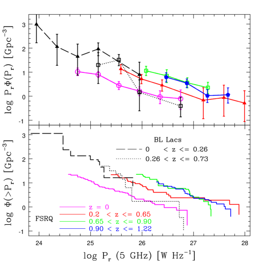
Figure 14.— Top: the differential radio luminosity function in a $P\times\phi(P)$ form for BL Lacs (black) in two redshift bins ($0-0.26$; dashed and $0.26-0.73$; dotted lines) and FSRQ in three redshift bins: $0.2-0.65$ (red), $0.65-0.90$ (green), $0.90-1.22$ (blue) and at $z=0$ (magenta). The latter is based on the $z\leq 1$ sub-sample and was de-evolved to zero redshift using the appropriate evolutionary parameter (see § 6.2 and Tab. 2). Error bars correspond to $1\sigma$ Poisson errors (Gehrels, 1986). Bottom: the integral radio luminosity function of BL Lacs in two redshift bins (dashed and dotted lines) and FSRQ in three redshift bins and at $z=0$.

A few interesting points can be made: 1. the different evolutionary properties of FSRQ and BL Lacs are visually apparent. Namely, splitting the BL Lac LF into two redshift bins is equivalent to a simple luminosity split, with the two LFs overlapping without discontinuity (see Beckmann et al., 2003, for a similar result in the X-ray band). The FSRQ LFs, on the other hand, clearly display an “evolution”, with the LFs in different redshift bins being shifted with respect to one another, as already discussed in § 6.2; 2. BL Lacs are $\sim 50$ times more numerous than FSRQ, the former having a total number density $\sim 1,100$ Gpc^-3 for $P_{\rm r}>7\times 10^{23}$ W/Hz, the latter having a total number density $\sim 23$ Gpc^-3 for $P_{\rm r}>4\times 10^{24}$ W/Hz. This is not simply due to the fact that BL Lacs reach lower powers, as the BL Lac number density above $4\times 10^{24}$ W/Hz is $\sim 240$ Gpc^-3, i.e., a factor $\sim 10$ larger than that of FSRQ above the same radio power, due to the fact that the FSRQ LF is flatter than that of BL Lacs ($\phi(P_{\rm r})\propto P_{\rm r}^{-1.7}$ vs. $\phi(P_{\rm r})\propto P_{\rm r}^{-2.1}$). The fact that FSRQ are $\approx 8$ times more abundant in our sample (§ 4) is due to the fact that FSRQ evolve, which means they are more luminous and their fluxes are “boosted”, and to our flux limit. BL Lacs are in fact expected to “catch up” at lower radio fluxes, becoming the dominant blazar class below $\approx 2$ mJy (Padovani & Urry, 1992); 3. all of the above, including the rough overlap between FSRQ and BL Lac LF in the $10^{26}\lesssim P_{\rm r}\lesssim 10^{27}$ W/Hz regime, is in perfect accordance with the unified schemes of Urry & Padovani (1995) (see also Padovani, 1992). Namely, a scenario in which BL Lacs are beamed FR Is and FSRQ are beamed FR IIs explains the larger number densities, lower radio powers, and steeper LF of the former (see also Figs. 9 and 13).

Finally, the observed LFs constrain a possible evolutionary link between the two classes. It has in fact been suggested (e.g., Cavaliere & D’Elia, 2002; Böttcher & Dermer, 2002) that a “genetic” link might be present between FSRQ and BL Lacs, with some of the former switching from a short-lived, high accretion rate regime to a long-lived, low accretion rate regime. This would imply a decrease in the FSRQ number density at lower redshifts, which is not seen and goes also against the evidence discussed in § 5 (see Fig. 7). Fig. 14 shows in fact that the FSRQ LF evolves smoothly to $z=0$, while that of BL Lacs has no redshift dependence. One could then infer that any evolutionary connection between FSRQ and BL Lacs has then to be limited and cannot affect the bulk of the blazar population. One caveat, however, is that radio power makes up a very small fraction of the total, bolometric luminosity, and is also not likely to be related to the episodes of large accretion of cold gas discussed by Cavaliere & D’Elia (2002) and Böttcher & Dermer (2002).

7. Summary and Conclusions

We have used a well-defined, complete sample selected from the Deep X-ray Radio Blazar Survey (DXRBS) to probe the radio number counts, evolution, and luminosity functions of blazars down to 5 GHz fluxes ($\sim 50$ mJy) and powers ($\sim 10^{24}$ W/Hz) about one order of magnitude deeper than previously available. Our sample includes 129 flat-spectrum radio quasars (FSRQ) and 24 BL Lacs detected in the radio and X-ray bands over $\lesssim 2,000$ deg². Great care has been taken in assessing the completeness of the sample and the effects of its double X-ray/radio selection, which are relevant for other on-going surveys as well. Our main results can be summarized as follows:

1. Our number counts agree with previous estimates at higher radio fluxes; the surface densities of BL Lacs and FSRQ reach $\sim 0.06$ deg^-2 and $\sim 0.6$ deg^-2 respectively at $f_{\rm 5GHz}\sim 50$ mJy.

2. The two blazar sub-classes have different evolutionary properties. FSRQ evolve as strongly as optically selected quasars, at least up to redshift $\approx 1.5$, with evidence of no evolution and a decline in space density at higher redshifts for high-power sources. BL Lacs, on the other hand, do not evolve. This is true also for high-energy peaked BL Lacs (HBL), at variance with some previous results based on X-ray selected samples, which had found evidence of negative evolution. FSRQ and BL Lac redshifts are also widely different, with the former covering the $0.2-4.7$ range with $\langle z\rangle=1.82\pm 0.08$ and the latter having $0.04\leq z\leq 0.73$ and $\langle z\rangle=0.26\pm 0.04$.

3. The observed radio luminosity functions are in good agreement with the predictions of unified schemes, with FSRQ getting close to their expected minimum power ($\approx 5\times 10^{24}/(H_{0}/50)^{2}$ W/Hz). The idea that blazars are radio galaxies seen with their jets close to our line of sight seems then to work also at relatively low powers.

4. Despite the fact that the large majority of DXRBS blazars are FSRQ, BL Lacs are intrinsically $\sim 50$ times more numerous, again in agreement with unified schemes.

5. The observed relative numbers of HBL and LBL are different from those predicted by the so-called ”blazar sequence”. The LBL/HBL ratio is roughly constant and $\sim 6$ in the radio band, instead of the predicted decrease down to $\sim 2$ at our flux limits. The opposite behavior is seen in the X-ray band, where a marked (sevenfold) increase in the LBL/HBL ratio is observed going to lower fluxes, instead of the slight decrease expected. The available evidence supports a scenario in which HBL are intrinsically a small minority ($\approx 10\%$) of all BL Lacs.

References

- Antón & Browne (2005) Antón, S., & Browne, I. W. A. 2005, MNRAS, 356, 225
- Arshakian et al. (2006) Arshakian, T. G., Ros, E., & Zensus, J. A. 2006, A&A, 458, 397
- Avni & Bahcall (1980) Avni, Y., & Bahcall, J. N. 1980, ApJ, 235, 694
- Bassett et al. (2004) Bassett, L. C., Brandt, W. N., Schneider, D. P., Vignali, C., Chartas, G., & Garmire, G. P. 2004, AJ, 128, 523
- Beckmann et al. (2003) Beckmann, V., Engels, D., Bade, N., & Wucknitz, O. 2003, A&A, 401, 927
- Böttcher & Dermer (2002) Böttcher, M., & Dermer, C. D. 2002, ApJ, 564, 86
- Browne & Marchã (1993) Browne, I. W. A., & Marchã, M. J. M. 1993, MNRAS, 261, 795
- Caccianiga et al. (1999) Caccianiga, A., Maccacaro, T., Wolter, A., della Ceca, R., & Gioia, I. M. 1999, ApJ, 513, 51
- Caccianiga et al. (2002) Caccianiga, A., Maccacaro, T., Wolter, A., della Ceca, R., & Gioia, I. M. 2002, ApJ, 566, 181
- Caccianiga & Marchã (2004) Caccianiga, A., & Marchã, M. J. M. 2004, MNRAS, 348, 937
- Cavaliere & D’Elia (2002) Cavaliere, A., & D’Elia, V. 2002, ApJ, 571, 226
- Collinge et al. (2005) Collinge, M. J., et al. 2005, AJ, 129, 2542
- Condon et al. (1998) Condon, J. J., Cotton, W. D., Greisen, E. W., Yin, Q. F., Perley, R. A., Taylor, G. B., & Broderick, J. J. 1998, AJ, 115, 169
- Croom et al. (2004) Croom, S. M., Smith, R. J., Boyle, B. J., Shanks, T., Miller, L., Outram, P. J., & Loaring, N. S. 2004, MNRAS, 349, 1397
- della Ceca et al. (1992) della Ceca, R., Maccacaro, T., Gioia, I. M., Wolter, A., & Stocke, J. T. 1992, ApJ, 389, 491
- di Serego Alighieri et al. (1994) di Serego Alighieri, S., Danziger, J., Morganti, R., & Tadhunter, C. 1994, MNRAS, 269, 998
- Dickey & Lockman (1990) Dickey, J. M., & Lockman, F. J. 1990, ARA&A, 28, 215
- Dunlop & Peacock (1990) Dunlop, J. S., & Peacock, J. A. 1990, MNRAS, 247, 19
- Fossati et al. (1997) Fossati, G., Celotti, A., Ghisellini, G., & Maraschi, L., 1997, MNRAS, 289, 136
- Fossati et al. (1998) Fossati, G., Maraschi, L., Celotti, A., Comastri, A., & Ghisellini, G. 1998, MNRAS, 299, 433
- Gehrels (1986) Gehrels, N. 1986, ApJ, 303, 336
- Giommi et al. (2006) Giommi, P., Colafrancesco, S., Cavazzutti, E., Perri, M., & Pittori, C. 2006, A&A, 445, 843
- Giommi, Menna, & Padovani (1999) Giommi, P., Menna, M. T., Padovani, P. 1999, MNRAS, 310, 465
- Giommi & Padovani (1994) Giommi, P., & Padovani, P. 1994, MNRAS, 268, L51
- Giommi et al. (2005) Giommi, P., Piranomonte, S., Perri, M., & Padovani, P. 2005, A&A, 434, 385
- Gregory et al. (1996) Gregory, P. C., Scott, W. K., Douglas, K., & Condon, J. J. 1996, ApJS, 103, 427
- Griffith & Wright (1993) Griffith, M. R., & Wright, A. E. 1993, AJ, 105, 1666
- Jarvis & Rawlings (2000) Jarvis, M. J., & Rawlings, S. 2000, MNRAS, 319, 121
- Kühr et al. (1987) Kühr, H., Johnston, K. J., Odenwald, S., & Adlhoch, J. 1987, A&AS, 71, 493
- Kühr et al. (1981) Kühr, H., Witzel, A., Pauliny-Toth, I. I. K., & Nauber, U. 1981, A&AS, 45, 367
- Landt et al. (2002) Landt, H., Padovani, P., & Giommi, P. 2002, MNRAS, 336, 945
- Landt et al. (2004) Landt, H., Padovani, P., Perlman, E. S., & Giommi, P. 2004, MNRAS, 351, 83
- Landt et al. (2001) Landt, H., Padovani, P., Perlman, E., Giommi, P., Bignall, H., & Tzioumis, A. 2001, MNRAS, 323, 757 (Paper II)
- Landt et al. (2006) Landt, H., Perlman, E. S., & Padovani, P. 2006, ApJ, 637, 183
- Laurent-Muehleisen et al. (1999) Laurent-Muehleisen, S. A., Kollgaard, R. I., Feigelson, E. D., Brinkmann, W., & Siebert, J. 1999, ApJ, 525, 127
- Marchã et al. (1996) Marchã, M. J. M., Browne, I. W. A., Impey, C. D., & Smith, P. S. 1996, MNRAS, 281, 425
- Morris et al. (1991) Morris, S. L., Stocke, J. T., Gioia, I. M., Schild, R. E., Wolter, A., Maccacaro, T., & Della Ceca, R. 1991, ApJ, 380, 49
- Nieppola et al. (2006) Nieppola, E., Tornikoski, M., & Valtaoja, E. 2006, A&A, 445, 441
- Padovani (1992) Padovani, P. 1992, MNRAS, 257, 404
- Padovani (1997) Padovani, P. 1997, in Very High Energy Phenomena in the Universe, ed. Y. Giraud-Héraud & J. Trân Thanh Vân (Paris: Ed. Frontières), 7
- Padovani (2001) Padovani, P. 2001, in ASP Conf. Ser. 227, Blazar Demographics & Physics, ed. P. Padovani, & C. M. Urry (San Francisco: ASP), 163
- Padovani (2002) Padovani, P. 2002, in Blazar Astrophysics with BeppoSAX and Other Observatories, ed. P. Giommi, E. Massaro, & G. Palumbo (Frascati: ASI), 101
- Padovani (2007) Padovani, P. 2007, in The Multi-messenger approach to high energy gamma-ray sources, Barcelona, July 4 – 7, 2006, in press (arXiv:astro-ph/0610545)
- Padovani et al. (2002) Padovani, P., Costamante, L., Ghisellini, G., Giommi, P., & Perlman, E. 2002, ApJ, 581, 895
- Padovani & Giommi (1995a) Padovani, P., & Giommi, P. 1995a, ApJ, 444, 567
- Padovani & Giommi (1995b) Padovani, P., & Giommi, P. 1995b, MNRAS, 277, 1477
- Padovani & Giommi (1996) Padovani, P., & Giommi, P. 1996, MNRAS, 279, 526
- Padovani, Giommi, & Fiore (1997) Padovani, P., Giommi, P., & Fiore, F. 1997, Mem. Soc. Astron. Italiana, 68, 147
- Padovani et al. (2003) Padovani, P., Perlman, E. S., Landt, H., Giommi, P., & Perri, M. 2003, ApJ, 588, 128
- Padovani & Urry (1990) Padovani, P., & Urry, C. M. 1990, ApJ, 356, 75
- Padovani & Urry (1992) Padovani, P., & Urry, C. M. 1992, ApJ, 387, 449
- Perlman et al. (1998) Perlman, E. S., Padovani, P., Giommi, P., Sambruna, R., Jones, L. R., Tzioumis, A., & Reynolds, J. 1998, AJ, 115, 1253 (Paper I)
- Perlman et al. (1996) Perlman, E. S., et al. 1996, ApJS, 104, 251
- Rector et al. (2000) Rector, T. A., Stocke, J. T., Perlman, E. S., Morris, S. L., & Gioia, I. M. 2000, AJ, 120, 1626
- Ricci et al. (2006) Ricci, R., Prandoni, I., Gruppioni, C., Sault, R. J., & de Zotti, G. 2006, A&A, 445, 465
- Schmidt (1968) Schmidt, M. 1968, ApJ, 151, 393
- Siebert et al. (1998) Siebert, J., Brinkmann, W., Drinkwater, M. J., Yuan, W., Francis, P. J., Peterson, B. A., & Webster, R. L. 1998, MNRAS, 301, 261
- Spergel et al. (2003) Spergel, D. N., et al. 2003, ApJS, 148, 175
- Stickel et al. (1993) Stickel, M., C. M., Fried, J. W., & Kühr, H. 1993, A&AS, 97, 483
- Stickel et al. (1994) Stickel, M., C. M., Fried, J. W., & Kühr, H. 1994, A&AS, 105, 211
- Stickel et al. (1991) Stickel, M., Padovani, P., Urry, C. M., Fried, J. W., & Kühr, H. 1991, ApJ, 374, 431
- Stocke et al. (1991) Stocke, J. T., Morris, S. L., Gioia, I. M., Maccacaro, T., Schild, R., Wolter, A., Fleming, T. A., & Henry, J. P. 1991, ApJS, 76, 813
- Urry & Padovani (1995) Urry, C. M., & Padovani, P. 1995, PASP, 107, 803
- Urry et al. (1991) Urry, C. M., Padovani, P., & Stickel, M. 1991, ApJ, 382, 501
- Urry et al. (2000) Urry, C. M., Scarpa, R., O’Dowd, M., Falomo, R., Pesce, J. E., & Treves, A. 2000, ApJ, 532, 816
- Wall et al. (2005) Wall, J. V., Jackson, C. A., Shaver, P. A., Hook, I. M., & Kellermann, K. I. 2005, A&A, 434, 133
- Wall & Peacock (1985) Wall, J. V., & Peacock, J. A. 1985, MNRAS, 216 173
- White, Giommi, & Angelini (1995) White, N. E., Giommi, P., & Angelini, L. 1995, database at http://wgacat.gsfc.nasa.gov
- White & Becker (1992) White, R. L., & Becker, R. H. 1992, ApJS, 79, 331