ESC observations of SN 2005cf
I. Photometric Evolution of a Normal Type Ia Supernova

Abstract

We present early–time optical and near–infrared photometry of supernova (SN) 2005cf. The observations, spanning a period from about 12 days before to 3 months after maximum, have been obtained through the coordination of observational efforts of various nodes of the European Supernova Collaboration and including data obtained at the 2m Himalayan Chandra Telescope. From the observed light curve we deduce that SN 2005cf is a fairly typical SN Ia with a post–maximum decline ($\Delta m_{15}(B)_{true}$ = 1.12) close to the average value and a normal luminosity of $M_{B,max}$ = –19.39$\pm$0.33. Models of the bolometric light curve suggest a synthesised ⁵⁶Ni mass of about 0.7M_⊙. The negligible host galaxy interstellar extinction and its proximity make SN 2005cf a good Type Ia supernova template.

1 Introduction

Type Ia supernovae (SNe Ia) have been extensively studied in recent years for their important cosmological implications. They are considered to be powerful distance indicators because they combine a high luminosity with relatively homogeneous physical properties. Moreover, observations of high–redshift SNe Ia have provided the clue for discovering the presence of a previously undetected cosmological component with negative pressure, labelled “dark energy”, and responsible of the accelerated expansion of the Universe (see Astier et al., 2006, and references therein).

Thanks to the collection of a larger and larger compendium of new data (e.g. Hamuy et al., 1996; Riess et al., 1999a ; Jha et al., 2006), an unexpected variety in the observed characteristics of SNe Ia has been shown to exist, and it is only using empirical relations between luminosity and distance–independent parameters, e.g. the shape of the light curve (see e.g. Phillips et al., 1993), that SNe Ia can be used as standardisable candles.

Actually Benetti et al., (2005) have recently shown that a one–parameter description of SNe Ia does not account for the observed variety of these objects. In order to understand the physical reasons that cause the intrinsic differences in Type Ia SNe properties, we need to improve the statistics by studying in detail a larger number of nearby objects. There are considerable advantages in analysing nearby SNe: one can obtain higher signal–to–noise (S/N) data, and these SNe can be observed for a longer time after the explosion, providing more information on the evolution during the nebular phase. Moreover, due to their proximity, the host galaxies are frequently monitored by automated professional SN searches and/or individual amateur astronomers. This significantly increases the probability of discovering very young SNe Ia, allowing the study of these objects at the earlier phases after the explosion.

In order to constrain the explosion and progenitor models, excellent–quality data of a significant sample of nearby SNe Ia is necessary. To this end, a large consortium of groups, comprising both observational and modelling expertise has been formed (European Supernova Collaboration, ESC) as part of a European Research Training Network (RTN).

To date, we obtained high–quality data for about 15 nearby SNe Ia. Analyses of individual SNe include SN 2002bo (Benetti et al., 2004), SN 2002er (Pignata et al., 2004; Kotak et al., 2005), SN 2002dj (Pignata et al., in preparation), SN 2003cg (Elias–Rosa et al., 2006), SN 2003du (Stanishev et al., 2007), SN 2003gs (Kotak et al., in preparation), SN 2003kf (Salvo et al., in preparation), SN 2004dt (Altavilla et al., in preparation) and SN 2004eo (Pastorello et al., 2007). Statistical analysis of samples of SNe Ia, including those followed by the ESC were performed by Benetti et al., (2005), Mazzali et al., (2005), Hachinger et al., (2006).

The proximity of SN 2005cf and its discovery almost two weeks before the $B$-band maximum (see below) made it an ideal target for the ESC. Immediately following the discovery announcement, we started an intensive photometric and spectroscopic monitoring campaign, which covered the SN evolution over a period of about 100 days from the discovery. This is the first of two papers where ESC data of SN 2005cf are presented. This work is devoted to study the early time optical and IR photometric observations of SN 2005cf, while spectroscopic data will be presented in a forthcoming paper (Garavini et al., 2007).

The layout of this paper is as follows: in Sect. 2 the ESC observations of SN 2005cf will be presented, including a description of the data reduction techniques. In Sect. 3 the light curves of SN 2005cf will be displayed and analysed. In Sect. 4 we derive the main parameters of the SN using empirical relations from literature, while in Sect. 5 additional properties are inferred from light curve modelling. We conclude the paper with a summary (Sect. 6).

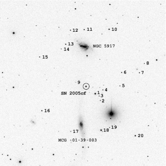
Figure 1: SN 2005cf in MCG –01–39–003: $B$ band image obtained on July 1, 2005 with the 2.2m Telescope of Calar Alto equipped with CAFOS. The field of view is 9$\times$9 arcmin². The sequence stars of Tab. 2 are labelled with numbers. The galaxy below the SN in the image is MCG –01–39–003, the upper one is NGC 5917. North is up, East is to the left.

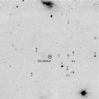
Figure 2: SN 2005cf in MCG –01–39–003: $H$ band image obtained on July 14, 2005 with the Telescopio Nazionale Galileo (TNG) of La Palma (Canary Islands) equipped with NICS. The field of view is 4.2$\times$4.2 arcmin². The NIR sequence stars reported in Tab. 3 are labelled. North is up, East is to the left.

2 Observations

2.1 SN 2005cf and the Host Galaxy

SN 2005cf was located close to the tidal bridge between two galaxies. It is known that the interaction between galaxies and/or galaxy activity phenomena may enhance the rate of star formation. As a consequence the rate of SNe in such galaxies is expected to increase. Although this scenario should favour mainly core–collapse SNe descending from short–lived progenitors, it could also increase the number of progenitors of SNe Ia with respect to the genuinely old stellar population (Della Valle & Livio, 1994). Indeed Smirnov & Tsvetkov, (1981) found indications of enhanced production of SNe of all types in interacting galaxy systems and Navasardyan et al., (2001) obtained a similar result in interacting pairs. More recently Della Valle et al., (2005) found evidence of an enhanced rate of SNe Ia in radio–loud galaxies, probably due to repeated episodes of interaction and/or merging. However, in general, the location of SN explosions does not seem to coincide with regions of strong interaction in the galaxies (Navasardyan et al., 2001), and the discovery of SNe in tidal tails remains an exceptional event (Petrosian & Turatto, 1995). This makes SN 2005cf a very interesting case.

SN 2005cf was discovered by H. Pugh and W. Li with the KAIT telescope on May 28.36 UT when it was at magnitude 16.4 (Puckett et al., 2005). Puckett et al., (2005) also report that nothing was visible on May 25.37 UT to a limiting magnitude of 18.5. The coordinates of SN 2005cf are $\alpha=15^{h}21^{m}32\aas@@fstack{s}21$ and $\delta=-07\degr 24\arcmin 47\aas@@fstack{\prime\prime}5$ (J2000). The object is located 15”.7 West and 123” North of the centre of MCG –01–39–003 (Fig. 1), a peculiar S0 galaxy (source NED).

SN 2005cf lies in proximity of a luminous bridge connecting MCG –01–39–003 with the Sb galaxy MCG –01–39–002 (also known as NGC 5917, see Fig. 1). This makes the association to one or the other galaxy uncertain. We will assume that SN 2005cf exploded in MCG –01–39–003, in agreement with Puckett et al., (2005), remarking that such assumption has no significant effect on the overall SN properties. Basic information on SN 2005cf, its host galaxy and the interacting companion is listed in Tab. 1.

Modjaz et al., (2005) obtained a spectrum on May 31.22 UT with the Whipple Observatory 1.5-m telescope (+ FAST) and classified the new object as a young (more than 10 days before maximum light) Type Ia SN. This gave the main motivation for the activation of the follow–up campaign by the ESC.

Table 1: Main parameters for SN 2005cf, the host galaxy MCG –01–39–003 and the interacting companion NGC 5917.

SN 2005cf
$\alpha$ (J2000.0)	15h21m32$\aas@@fstack{s}$21	1
$\delta$ (J2000.0)	-07$\degr$24$\arcmin$47$\aas@@fstack{\prime\prime}$.5	1
Offset Galaxy–SN‡	15′′.7W, 123′′N	1
SN Type	Ia	2
E$(B-V)_{host}$	0	3
E$(B-V)_{Gal}$	0.097	4
Discovery date (UT)	2005 May 28.36	1
Discovery JD	2453518.86	1
Discovery mag.	16.4	1
Predisc. limit epoch (UT)	2005 May 25.37	1
Predisc. limit mag.	18.5	1
JD($B_{max}$)	2453534.0	3
$B_{max}$	13.54	3
$M_{B,max}(\mu)$	$-$19.39	3
$\Delta$m${}_{15}(B)_{true}$	1.12	3
$s^{-1}$	0.99	3
$\Delta$$C_{12}$	0.355	3
tr	18.6	3
M(56Ni)	0.7M⊙	3
MCG –01–39–003
PGC name	PGC 054817	5
Galaxy type	S0 pec	5
$\alpha$ (J2000.0)	15h21m33$\aas@@fstack{s}$29	5
$\delta$ (J2000.0)	$-07\degr 26\arcmin 52\aas@@fstack{\prime\prime}38$	5
$B_{tot}$	14.75 $\pm$ 0.43	6
D	$1\arcmin 4\times 0\arcmin 7$	5
vVir	1977 km s-1	6
v3k	2114 km s-1	6
$\mu$	32.51	3
E$(B-V)_{Gal}$	0.098	4
MCG –01–39–002 (NGC 5917)
PGC name	PGC 054809	5
Galaxy type	Sb pec	5
$\alpha$ (J2000.0)	15h21m32$\aas@@fstack{s}$57	5
$\delta$ (J2000.0)	$-07\degr 22\arcmin 37\aas@@fstack{\prime\prime}8$	5
$B_{tot}$	13.81 $\pm$ 0.50	6
D	$1\arcmin 5\times 0\arcmin 9$	5
vvir	1944 km s-1	6
v3k	2080 km s-1	6
$\mu$	32.51	3
E$(B-V)_{Gal}$	0.095	4

^‡ we assume MCG –01–39–003 as host galaxy.
1 = Puckett et al., (2005); 2 = Modjaz et al., (2005);
3 = this paper; 4 = Schlegel et al., (1998);
5 = NED (it http://nedwww.ipac.caltech.edu);
6 = LEDA (it http://leda.univ-lyon1.fr).

2.2 ESC Observations

Table 2: $U$, $B$, $V$, $R$, $I$ magnitudes of the sequence stars in the field of SN 2005cf. The errors reported in brackets are the r.m.s. of the available measurements, obtained during photometric nights only.

Star	$U$	$B$	$V$	$R$	$I$
1	14.886 (0.018)	14.710 (0.008)	13.986 (0.007)	13.561 (0.007)	13.155 (0.006)
2	18.243 (0.021)	18.125 (0.008)	17.308 (0.007)	16.867 (0.008)	16.453 (0.006)
3	19.217 (0.015)	18.292 (0.009)	17.262 (0.007)	16.682 (0.008)	16.178 (0.006)
4	18.080 (0.020)	17.548 (0.011)	16.661 (0.007)	16.164 (0.008)	15.705 (0.006)
5	19.290 (0.013)	18.131 (0.009)	16.705 (0.005)	15.800 (0.005)	14.930 (0.007)
6		17.176 (0.008)	17.005 (0.008)	16.940 (0.012)	16.829 (0.007)
7	17.314 (0.020)	17.172 (0.010)	16.350 (0.006)	15.895 (0.008)	15.436 (0.006)
8	19.128 (0.022)	18.207 (0.009)	17.152 (0.008)	16.552 (0.006)	16.035 (0.007)
9	20.984 (0.059)	19.776 (0.010)	18.490 (0.012)	17.605 (0.007)	16.795 (0.006)
10	15.865 (0.009)	15.827 (0.011)	15.169 (0.007)	14.777 (0.005)	14.423 (0.006)
11	16.917 (0.010)	16.929 (0.006)	16.264 (0.007)	15.883 (0.006)	15.523 (0.010)
12	17.475 (0.011)	17.503 (0.008)	16.837 (0.007)	16.458 (0.007)	16.109 (0.005)
13	17.668 (0.016)	16.688 (0.008)	15.662 (0.007)	15.066 (0.006)	14.573 (0.009)
14	19.939 (0.018)	18.879 (0.009)	17.271 (0.010)	16.300 (0.008)	15.167 (0.010)
15	17.627 (0.011)	17.398 (0.009)	16.543 (0.009)	16.058 (0.008)	15.602 (0.005)
16	16.446 (0.011)	16.401 (0.010)	15.700 (0.007)	15.288 (0.006)	14.909 (0.008)
17	18.181 (0.016)	18.456 (0.009)	17.863 (0.007)	17.487 (0.009)	17.153 (0.007)
18	15.228 (0.019)	14.717 (0.008)	13.833 (0.006)	13.298 (0.006)	12.786 (0.008)
19	17.808 (0.013)	17.952 (0.008)	17.397 (0.009)	17.031 (0.007)	16.695 (0.007)
20	16.556 (0.022)	15.813 (0.006)	14.801 (0.005)	14.201 (0.005)	13.676 (0.007)

Table 3: $J$, $H$, $K^{\prime}$ magnitudes of the sequence stars in the field of SN 2005cf, with assigned errors.

Star	$J$	$H$	$K^{\prime}$
1	12.54 (0.01)	12.15 (0.02)	12.21 (0.01)
2	15.91 (0.01)	15.46 (0.02)	15.53 (0.03)
3	15.49 (0.01)	14.97 (0.01)	14.99 (0.02)
4	15.10 (0.02)	14.61 (0.02)	14.60 (0.01)
5	13.84 (0.08)	13.22 (0.01)	13.25 (0.03)
6	16.74 (0.01)	16.50 (0.01)
9	15.80 (0.01)	15.07 (0.03)	15.01 (0.02)
A	16.56 (0.03)	15.88 (0.04)	15.85 (0.04)
B	16.85 (0.03)	16.27 (0.03)	16.12 (0.01)
C	17.70 (0.03)	17.31 (0.02)	17.34 (0.01)
D	17.77 (0.03)	17.36 (0.04)	17.40 (0.01)
E	17.62 (0.01)	17.26 (0.02)	17.27 (0.07)
F	17.39 (0.01)	17.26 (0.07)

We have obtained more than 360 optical data points, covering about 60 nights, from about 12 days before the $B$ band maximum to approximately 3 months after. In addition, near–infrared (NIR) observations have been performed in 5 selected epochs. Observations at late phases will be presented in a forthcoming paper.

During the follow–up, 8 different instruments have been used for the optical and 2 for the NIR observations:

• the 40–inch Telescope at the Siding Spring Observatory (Australia) with a Wide Field Camera (eight 2048$\times$4096 CCDs, with pixel scale of 0.375 arcsec pixel^-1) and standard broad band Bessell filters $B$, $V$, $R$, $I$;

• the 3.58m Italian Telescopio Nazionale Galileo (TNG) at the Observatorio de los Muchachos in La Palma (Canary Islands, Spain), equipped with DOLORES and a Loral thinned and back–illuminated 2048$\times$2048 detector, with scale 0.275 arcsec pixel^-1, yielding a field of view of about 9.4$\times$9.4 arcmin². We used the $U$, $B$, $V$ Johnson and $R$, $I$ Cousins filters (with TNG identification numbers 1, 10, 11, 12, 13, respectively);

• the 2.5m Nordic Optical Telescope in La Palma equipped with ALFOSC (with an E2V 2048$\times$2048 CCD of 0.19 arcsec pixel^-1) and a set of $U$, $B$, $V$, $R$ Bessell filters (with NOT identification numbers 7, 74, 75, 76, respectively) and an interference $i$ band filter (number 12);

• the 2.3m Telescope in Siding Spring, equipped with the E2V 2048$\times$2048 imager, with pixel scale of 0.19 arcsec pixel^-1 and standard broad band Bessell filters $U$, $B$, $V$, $R$, $I$;

• the Mercator 1.2m Telescope in La Palma, equipped with a 2048$\times$2048 CCD camera (MEROPE) having a field of view of 6.5$\times$6.5 arcmin² and a resolution of about 0.19 arcsec pixel^-1. We used $U$, $B$, $V$, $R$, $I$ filters (with identification codes UG, BG, VG, RG and IC, respectively);

• the 2.2m Telescope of Calar Alto (Spain) equipped with CAFOS and a SITe 2048$\times$2048 CCD, 0.53 arcsec pixel^-1; the filters available were the $U$, $B$, $V$, $R$, $I$ Johnson (labelled as 370/47b, 451/73, 534/97b, 641/158, 850/150b, respectively);

• the Copernico 1.82m Telescope of Mt. Ekar (Asiago, Italy); equipped with AFOSC, a TEKTRONIX 1024$\times$1024 thinned CCD (0.47 arcsec pixel^-1) and a set of $B$, $V$, $R$ Bessell and the $i$ Gunn filters;

• the ESO/MPI 2.2m Telescope in La Silla (Chile), with a wide field mosaic of eight 2048$\times$4096 CCDs (0.24 arcsec pixel^-1) and a total field of view of 34$\times$33 arcmin². We used the broad band filters $U$ (labelled as ESO877), $B$ (ESO878), $V$ (ESO843), Cousins $Rc$ (ESO844), and EIS $I$ (ESO879);

• the TNG equipped with the Near Infrared Camera Spectrometer (NICS) with a HgCdTe Hawaii 1024$\times$1024 array (field of view 4.2$\times$4.2 arcmin², scale 0.25 arcsec pixel^-1); the filters used in the observations were $J$, $H$, $K^{\prime}$.

• the 3.5m Telescope in Calar Alto with Omega–Cass, having a Rockwell 1024$\times$1024 HgCdTe Hawaii array with pixel scale 0.2 arcsec pixel^-1 and $J$, $H$, $K^{\prime}$ filters.

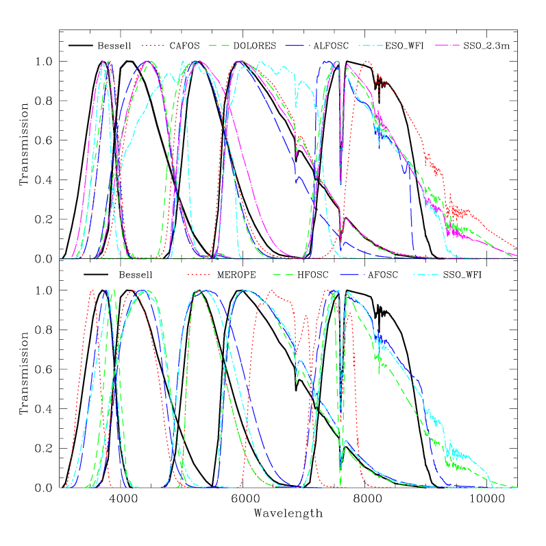
Figure 3: Comparison between the different instrumental $U$, $B$, $V$, $R$ and $I$ transmission curves, normalised to the peak transmission, and the standard Johnson–Cousins functions. The instrumental transmission curves were reconstructed taking into account the filter transmission, the CCD quantum efficiency, the reflectivity of the mirrors, the atmospheric transmission and, when available, the lenses throughput.

In this paper we also included the data from Anupama et al. (in preparation) obtained using the 2m Himalayan Chandra Telescope (HCT) of the Indian Astronomical Observatory (IAO), Hanle (India), equipped with the Himalaya Faint Object Spectrograph Camera (HFOSC), with a SITe 2048$\times$4096 CCD (pixel scale 0.296 arcsec pixel^-1), with a central region (2048$\times$2048 pixels) used for imaging and covering a field of view of 10$\times$10 arcmin². Standard Bessell $U$, $B$, $V$, $R$, $I$ filters were used.

The $U$, $B$, $V$, $R$, $I$ transmission curves for all optical instrumental configurations used during the follow–up of SN 2005cf are shown in Fig. 3, and compared with the standard Johnson–Cousins passbands (Bessell, 1990).

Table 4: Comparison between synthetic and photometric colour terms. The colour terms for HFOSC are provided by the observatory without associated errors. For SSO–40inch Telescope + WFI, we have only two colour term measurements, therefore the statistic is too poor to compute reliable errors.

Instrument                   $U$ $(U-B)$                                      $B$ $(B-V)$                                     $V$ $(B-V)$                                      $R$ $(V-R)$                                      $I$ $(R-I)$
	syn	ph	syn	ph	syn	ph	syn	ph	syn	ph
40inch+WFI			$-$0.022	0.005	$-$0.002	0.033	0.054	0.054	0.042	$-$0.019
DOLORES	0.059$\star$	0.105 $\pm$ 0.047	0.080	0.064 $\pm$ 0.018	$-$0.101	$-$0.120 $\pm$ 0.033	0.031	0.022$\pm$ 0.037	0.025	0.023 $\pm$ 0.017
ALFOSC	0.093$\star$	0.122 $\pm$ 0.010	0.023	0.044 $\pm$ 0.012	$-$0.048	$-$0.049 $\pm$ 0.021	$-$0.074	$-$0.098 $\pm$ 0.024	$-$0.086	$-$0.068 $\pm$ 0.033
2.3m+imager	0.048	0.094 $\pm$ 0.033	0.081	0.014 $\pm$ 0.024	0.026	0.027 $\pm$ 0.009	0.035	0.040 $\pm$ 0.016	0.028	0.002 $\pm$ 0.016
Merope	$-$0.089	$-$0.105 $\pm$ 0.008	$-$0.168	$-$0.130 $\pm$ 0.014	$-$0.002	$-$0.001 $\pm$ 0.011	0.126	0.134 $\pm$ 0.022	$-$0.284	$-$0.332 $\pm$ 0.026
CAFOS	0.121$\star$	0.167 $\pm$ 0.016	0.107	0.115 $\pm$ 0.005	$-$0.061	$-$0.048 $\pm$ 0.005	$-$0.008	$-$0.015 $\pm$ 0.017	0.219	0.256 $\pm$ 0.036
AFOSC			$-$0.068$\star$	$-$0.030 $\pm$ 0.013	0.041	0.047 $\pm$ 0.010	0.066	0.052 $\pm$ 0.033	$-$0.031	$-$0.044 $\pm$ 0.036
2.2m+WFI	$-$0.021	$-$0.070 $\pm$ 0.036	0.249	0.244 $\pm$ 0.024	$-$0.067	$-$0.067 $\pm$ 0.013	0.015	0.000 $\pm$ 0.022	$-$0.010	0.006 $\pm$ 0.022
HFOSC	0.155	0.188	$-$0.028	$-$0.049	0.045	0.047	0.038	0.065	0.018	0.017

$\star$  The passband’s blue cutoff was modified

2.3 Data Reduction

The reduction of the optical photometry was performed using standard IRAF tasks. The first reduction steps included bias, overscan and flat field corrections, and the trimming of the images using the IRAF package CCDRED.

The pre–reduction of the NIR images was slightly more laborious, as it required a few additional steps. Due to the high luminosity of the night sky in the NIR, we needed to remove the sky contribution from the target images, by creating “clean” sky images. This was done by median–combining a number of dithered science frames. The resulting sky template image was then subtracted from the target images. Most of our data were obtained with several short–exposure dithered frames, which had to be spatially registered and then combined in order to improve the S/N.

The NICS images required particular treatment, as they needed also to be corrected for the cross talking effect (i.e. a signal which was detected in one quadrant produced negative ghost images in the other 3 quadrants) and for the distortion of the NICS optics. These corrections were performed using a pipeline, SNAP, available at TNG for the reduction of images obtained using NICS.

Instrumental magnitudes of SN 2005cf were determined with the point–spread function (PSF) fitting technique, performed using the SNOoPY package. Since SN 2005cf is a very bright and isolated object, the subtraction of the host galaxy template is not required, and the PSF fitting technique provides excellent results.

In order to transform instrumental magnitudes into the standard photometric system, first–order colour corrections were applied, using colour terms derived from observations of several photometric standard fields (Landolt, 1992). The photometric zeropoints were finally determined for all nights by comparing magnitudes of a local sequence of stars in the vicinity of the host galaxy (cf. Fig. 1) to the average estimates obtained during some photometric nights. The average magnitudes for the sequence stars in the field of SN 2005cf are reported in Tab. 2.

The HFOSC data from Anupama et al. have been checked comparing the stars in common to both local sequences. In order to calibrate their SN magnitudes onto our sequence, we applied additive zeropoint shifts (smaller than 0.05 mags), slightly corrected for the colour terms of the instrumental configuration of HCT.

In analogy to optical observations, NIR photometry was computed using different standard fields of the Arnica catalogue (Hunt et al., 1998) and finally calibrated using a number of local standards in the field of SN 2005cf (Fig. 2). The $J$, $H$, $K^{\prime}$ magnitudes of the IR local standards are reported in Tab. 3.

3 Light Curves of SN 2005cf

3.1 S–Correction to the Optical Light Curves

The optical photometry of SN 2005cf, as derived from comparison with the Landolt’s standard fields and our local sequence stars only (see below), shows a disturbing scatter in the magnitudes obtained using different instrumental configurations. This was due to the combination of the difference between the instrumental photometric system (see also Fig. 3) and the non–thermal SN spectrum. In order to remove these systematic errors we used a technique, presented in Stritzinger et al., (2002), called S–correction. To compute the corrections, one first needs to determine the instrumental passband $S(\lambda)$, defined as:

$$S(\lambda)=F(\lambda)\cdot QE(\lambda)\cdot A(\lambda)\cdot M(\lambda)\cdot L(\lambda)$$ (1)

where $F(\lambda)$ is the filter transmission function, $QE(\lambda)$ is the detector quantum efficiency, $A(\lambda)$ is the continuum atmospheric transmission profile, $M(\lambda)$ is the mirror reflectivity function and $L(\lambda)$ is the lens throughput. Information on instruments, detectors and filters used during the follow–up of SN 2005cf is given in Sect. 2.2. In order to derive the atmospheric transmission profile of Calar Alto and La Palma, we made use of the information reported in Hopp & Fernàndez, (2002) and King, (1985), respectively, while for the La Silla site we used the CTIO transmission curve available in IRAF. For Asiago–Ekar, the Siding Spring Observatory and the Indian Astronomical Observatory we obtained $A(\lambda)$ by adapting the standard atmospheric model proposed by Walker, (1987) in order to match the average broad band absorption coefficients of these sites. Finally, $M(\lambda)$ was obtained using a standard aluminum reflectivity curve multiplied by the number of reflections in a given instrumental configuration, while $L(\lambda)$ was estimated for DOLORES and WFI only. For all the other instrumental configurations, we assumed that $L(\lambda)$ was constant across the whole spectral range. This approximation, together with a rapid variability both in the CCD quantum efficiency and in the atmosphere’s transmission curve at the blue wavelengths, are probably the reasons why the $U$ reconstructed passbands do not match the observed ones (see Tab. 4).

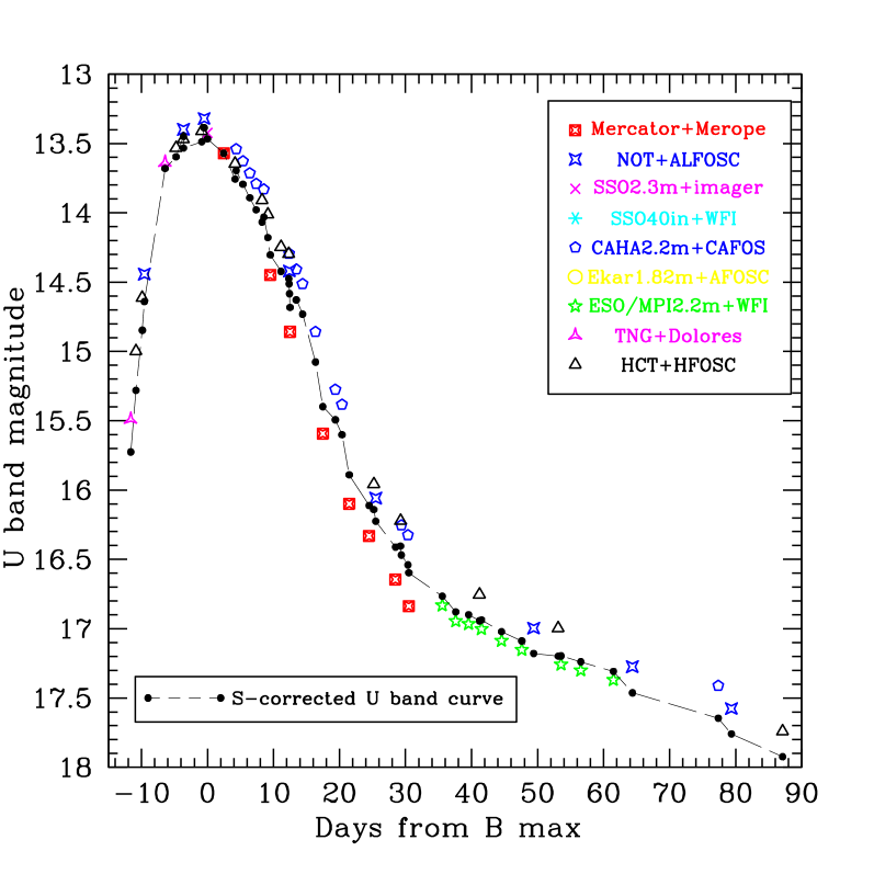
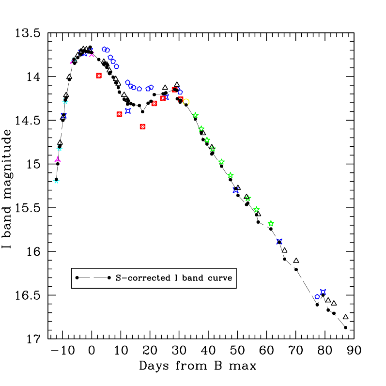
Figure 4: Top: comparison between the original $U$ band light curve of SN 2005cf and the S–corrected one. Bottom: the same, but for the $I$ band. Original data points obtained using different instruments are plotted with different symbols. The large scatter is due to the diversity of the $U$ and $I$ filters available at the various telescopes. The final, S–corrected $U$ and $I$ band photometry is represented by filled circles, connected with a dashed line.

In order to check the match between the modelled passbands and the real ones, and to calculate the instrumental zero points for all configurations, we followed the same approach as Pignata et al., (2004), updating to the new set of spectro–photometric standard stars from Stritzinger et al., (2005), which span a range in colour larger than that provided by previous works (e.g. Hamuy et al., 1994). In Tab. 4 we report the comparison between the colour terms computed via the synthetic photometry and those determined through the observation of a number of standard fields. For the latter, the estimates and their associated errors (see Tab. 4) were computed using a 3$\sigma$–clipped average. In a few cases, when the difference between the synthetic colour term and photometric colour term was larger than 3$\sigma$, the passbands were adjusted.

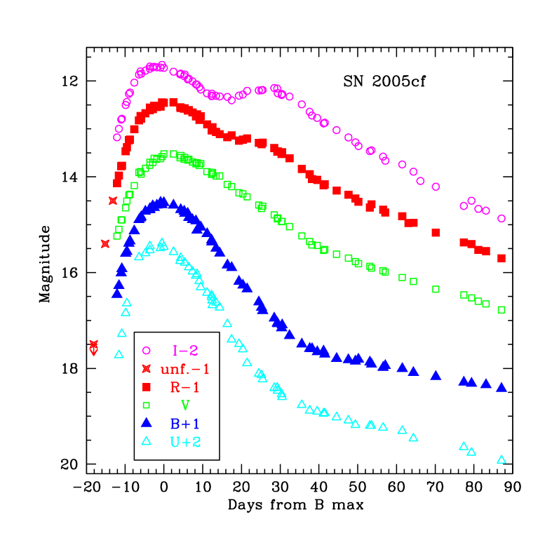
Figure 5: $U$, $B$, $V$, $R$, $I$ light curves of SN 2005cf, including the unfiltered measurements from IAU Circ. 8534 (asterisk). The phase is measured in days from the $B$ band maximum.

For each instrumental configuration, the S–correction measurements at different epochs were fitted by a third– or fourth–order polynomial, as in Pignata et al., (2004), and the r.m.s. deviations of the data points from the fitted law provided an estimate of the errors due to the correction itself. The correction applied to the photometry of SN 2005cf turned out to be effective because of the detailed characterisation of the photometric properties of most of the instruments used by the ESC (Pignata et al., 2004) and the excellent spectral sequence available for this object (Garavini et al., 2007). Note that, however, since most spectra of SN 2005cf had not adequate coverage in the region below 3500Å, we had to resort to spectra of SN 1994D in order to estimate the S–correction for the $U$ band.

The original (i.e. non S–corrected) optical photometry for SN 2005cf is reported in Tab. LABEL:SN_mags (columns 3 to 7). The corrections to be applied to the original magnitudes are also reported in Tab. LABEL:SN_mags (columns 8 to 12). The differences are in general quite small, especially in the $B$, $V$, $R$ bands, and they are significant only for some specific instrumental configurations (sometimes of 0.1–0.2 magnitudes, see e.g. the $I$ filters of the Mercator Telescope + Merope, the 2.2m Calar Alto Telescope + CAFOS and the Himalayan Chandra Telescope + HFOSC, or the $B$ filter mounted at the 2.2m ESO/MPI Telescope + WFI). On the contrary, the $U$ band correction is large for most instrumental configurations. As shown in Fig. 3 (see also Stanishev et al. 2006), this is because the sensitivity curves of the $U$ filters available at the various telescopes are significantly different (being often shifted to redder wavelengths) compared to the standard $U$ Bessell passband.

Table 5: continued.

Date	JD	Original Magnitude					S-correction					S
	(+2400000)	$U$	$B$	$V$	$R$	$I$	$\Delta U$	$\Delta B$	$\Delta V$	$\Delta R$	$\Delta I$
31/5	53521.90		15.493	15.243	15.142	15.191		-0.031	-0.005	-0.004	-0.014	1
31/5	53522.38	15.490	15.299	15.127	14.973	14.952	0.235	-0.027	-0.030	0.003	0.047	2
01/6	53522.97		15.044	14.902	14.785	14.819		-0.032	-0.004	-0.005	-0.014	1
01/6	53523.16	14.999	14.934	14.913	14.769	14.759	0.282	-0.010	-0.011	0.002	0.030	H
02/6	53524.13	14.613	14.609	14.658	14.466	14.472	0.234	-0.009	-0.009	0.001	0.029	H
02/6	53524.44	14.443	14.582	14.514	14.377	14.449	0.198	-0.021	-0.007	0.006	-0.011	3
03/6	53524.97		14.425	14.382	14.241	14.282		-0.033	-0.003	-0.005	-0.013	1
03/6	53525.25		14.348	14.373	14.224	14.214		-0.009	-0.006	0	0.028	H
04/6	53526.35		14.139	14.189	14.009	14.007		-0.008	-0.004	-0.002	0.028	H
06/6	53527.57	13.638	13.924	13.943	13.823	13.831	0.043	-0.026	-0.034	-0.001	0.035	2
06/6	53527.95		13.896	13.896	13.736	13.816		-0.034	-0.002	-0.006	-0.014	1
06/6	53528.14		13.848	13.944	13.792	13.822		-0.007	-0.001	-0.004	0.027	H
07/6	53529.24	13.533	13.730	13.822	13.680	13.758	0.063	-0.006	0.002	-0.005	0.027	H
08/6	53530.38	13.399	13.712	13.710	13.544	13.726	0.050	-0.018	-0.012	0.012	-0.029	3
08/6	53530.38	13.470	13.676	13.753	13.617	13.719	0.063	-0.006	0.003	-0.007	0.026	H
09/6	53531.12		13.614	13.695	13.597	13.688		-0.005	0.004	-0.007	0.025	H
09/6	53531.48		13.659	13.629		13.737		-0.017	-0.013		-0.034	3
10/6	53531.52				13.501					0.013		3
10/6	53532.19		13.601	13.628	13.553	13.689		-0.004	0.004	-0.008	0.025	H
11/6	53533.13	13.410	13.539	13.618	13.541	13.696	0.078	-0.004	0.004	-0.009	0.024	H
12/6	53533.50	13.320	13.602	13.592	13.432	13.706	0.067	-0.015	-0.012	0.015	-0.042	3
12/6	53533.99	13.423	13.568	13.525	13.462	13.748	0.044	-0.029	-0.002	-0.007	-0.022	4
14/6	53536.47	13.570	13.602	13.501	13.486	13.990	0.001	-0.008	0.022	-0.041	-0.184	5
16/6	53538.19	13.645		13.606	13.558	13.831	0.112		-0.005	-0.007	0.031	H
16/6	53538.36	13.540	13.725	13.581	13.562	13.688	0.155	-0.036	-0.023	0.004	0.158	6
17/6	53539.21		13.723	13.641	13.583	13.864		-0.003	-0.008	-0.007	0.033	H
17/6	53539.37	13.628	13.798	13.616	13.567	13.700	0.166	-0.034	-0.022	0.004	0.164	6
18/6	53540.13		13.770	13.664	13.625	13.931		-0.003	-0.010	-0.006	0.036	H
18/6	53540.41	13.714	13.887	13.656	13.607	13.780	0.178	-0.032	-0.021	0.004	0.172	6
19/6	53541.37	13.790	13.929	13.713	13.653	13.828	0.189	-0.030	-0.020	0.004	0.180	6
20/6	53542.26	13.909	13.925	13.743	13.742	14.030	0.158	-0.004	-0.016	-0.003	0.041	H
21/6	53542.53	13.831	14.144	13.724	13.695	13.885	0.201	-0.029	-0.019	0.004	0.189	6
21/6	53543.14	14.013	14.050	13.781	13.814	14.083	0.165	-0.005	-0.018	-0.001	0.043	H
22/6	53543.51	14.450	14.065	13.694	13.764	14.432	-0.146	-0.012	0.033	-0.028	-0.254	5
23/6	53545.13	14.246	14.197	13.915	13.906	14.212	0.177	-0.006	-0.023	0.001	0.047	H
24/6	53546.30	14.296	14.330	13.974	14.031	14.267	0.179	-0.007	-0.025	0.002	0.049	H
24/6	53546.36	14.294	14.386	13.921	13.974	14.067	0.219	-0.028	-0.012	0.004	0.198	6
24/6	53546.43	14.420	14.368	13.937	13.950	14.394	0.163	-0.007	0.003	0.022	-0.087	3
25/6	53546.50	14.859	14.376	13.879	13.986		-0.177	-0.014	0.036	-0.018		5
25/6	53547.45	14.409	14.523	13.996	14.060	14.111	0.219	-0.028	-0.010	0.004	-0.199	6
26/6	53548.40	14.512	14.626	13.990	14.105	14.126	0.219	-0.029	-0.009	0.005	0.197	6
28/6	53550.37	14.858	14.877	14.164	14.170	14.143	0.219	-0.033	-0.005	0.005	0.189	6
29/6	53551.48	15.593	14.919	14.169	14.143	14.573	-0.195	-0.019	0.036	-0.005	-0.170	5
01/7	53553.37	15.275	15.224	14.333	14.240	14.142	0.218	-0.040	0.001	0.006	0.164	6
02/7	53554.37	15.383	15.307	14.356	14.219	14.124	0.218	-0.042	0.003	0.007	0.159	6
03/7	53555.47	16.099	15.364	14.385	14.196	14.308	-0.209	-0.024	0.034	0.005	-0.101	5
06/7	53558.48	16.331	15.640	14.558	14.287	14.250	-0.220	-0.024	0.032	0.004	-0.053	5
07/7	53559.19	15.957	15.751	14.680	14.331	14.130	0.183	-0.025	-0.020	-0.011	0.062	H
07/7	53559.49	16.059	15.812	14.593	14.280	14.237	0.166	-0.015	0.021	0.007	-0.049	3
10/7	53562.48	16.645	15.972	14.763	14.402	14.151	-0.234	-0.020	0.031	-0.001	-0.004	5
11/7	53563.24	16.220	16.079	14.889	14.495	14.095	0.184	-0.026	-0.015	-0.018	0.062	H
11/7	53563.37	16.253	16.135	14.850	14.459	14.143	0.216	-0.067	0.011	0.010	0.113	6
12/7	53564.37	16.324	16.226	14.923	14.515	14.180	0.215	-0.068	0.011	0.010	0.114	6
Date	JD	Original Magnitude					S-correction					S
	(+2400000)	$U$	$B$	$V$	$R$	$I$	$\Delta U$	$\Delta B$	$\Delta V$	$\Delta R$	$\Delta I$
13/7	53564.50	16.837	16.113	14.902	14.492	14.260	-0.241	-0.018	0.031	-0.004	0.012	5
14/7	53566.41		16.327	15.066	14.633	14.291		-0.010	-0.024	-0.019	0.035	7
18/7	53569.57	16.831	16.592	15.179	14.863	14.444	-0.065	-0.096	0.056	-0.027	0.044	8
20/7	53571.60	16.945	16.684	15.298	14.977	14.599	-0.066	-0.097	0.054	-0.029	0.044	8
20/7	53572.21		16.616	15.430	15.071	14.650		-0.023	-0.009	-0.023	0.072	H
22/7	53573.55	16.965	16.753	15.384	15.097	14.727	-0.066	-0.097	0.051	-0.032	0.045	8
23/7	53575.20	16.753	16.660	15.546	15.204	14.810	0.190	-0.020	-0.008	-0.023	0.076	H
24/7	53575.51	17.002	16.799	15.471	15.193	14.827	-0.066	-0.096	0.048	-0.034	0.046	8
27/7	53578.55	17.086	16.891	15.574	15.327	14.977	-0.065	-0.094	0.043	-0.038	0.048	8
30/7	53581.61	17.152	16.914	15.659	15.417	15.129	-0.064	-0.091	0.039	-0.042	0.051	8
31/7	53583.41	16.996	16.862	15.755	15.443	15.299	0.182	-0.014	0.016	0.011	-0.018	3
01/8	53584.20		16.833	15.823	15.543	15.275		-0.022	-0.010	-0.020	0.084	H
04/8	53587.14	16.997	16.897	15.881	15.660	15.378	0.201	-0.025	-0.012	-0.018	0.086	H
05/8	53587.56	17.258	17.005	15.873	15.619	15.392	-0.062	-0.092	0.033	-0.044	0.056	8
08/8	53590.56	17.300	17.076	15.929	15.733	15.522	-0.061	-0.092	0.031	-0.044	0.059	8
08/8	53591.13		16.970	16.006	15.763	15.575		-0.027	-0.015	-0.016	0.089	H
13/8	53595.50	17.369	17.094	16.075	15.868	15.681	-0.061	-0.089	0.028	-0.043	0.062	8
14/8	53597.10				15.978					-0.012		H
15/8	53598.38	17.275	17.096	16.172	15.943	15.886	0.187	-0.008	0.014	0.018	0.009	3
17/8	53600.18					15.992					0.096	H
21/8	53604.15		17.192	16.368	16.173	16.109		-0.022	-0.020	-0.008	0.099	H
28/8	53611.38	17.410	17.294	16.475	16.372	16.518	0.235	-0.003	-0.008	-0.001	0.091	6
30/8	53613.37	17.576	17.293	16.519	16.385	16.464	0.183	0.023	0.008	0.020	0.036	3
01/9	53615.14			16.618	16.525	16.561			-0.020	0.001	0.109	H
03/9	53617.10		17.341	16.674	16.552	16.596		0	-0.020	0.003	0.112	H
07/9	53621.11	17.741	17.412	16.798	16.695	16.754	0.183	0.009	-0.020	0.007	0.116	H

1 = 40inch SSO Telescope + WFI;

2 = 3.5m Telescopio Nazionale Galileo + DOLORES;

3 = 2.5m Nordic Optical Telescope + ALFOSC;

4 = 2.3m SSO Telescope + Imager;

5 = 1.2m Mercator Telescope + MEROPE;

6 = 2.2m Calar Alto Telescope + CAFOS;

7 = 1.82m Copernico Telescope + AFOSC;

8 = 2.2m ESO/MPI Telescope + WFI;

H = 2m Himalayan Chandra Telescope + HFOSC.

Table 6: continued.

Date	JD	$U$	$B$	$V$	$R$	$I$	S
	(+2400000)
25/5	53515.87				$\geq$18.5		0
28/5	53518.86				16.4		0
30/5	53520.85				15.5		0
31/5	53521.90		15.462 (0.010)	15.238 (0.008)	15.138 (0.009)	15.177 (0.011)	1
31/5	53522.38	15.725 (0.043)	15.272 (0.015)	15.097 (0.010)	14.976 (0.011)	14.999 (0.024)	2
01/6	53522.97		15.012 (0.009)	14.898 (0.008)	14.780 (0.008)	14.805 (0.009)	1
01/6	53523.16	15.281 (0.055)	14.924 (0.017)	14.902 (0.020)	14.771 (0.013)	14.789 (0.024)	H
02/6	53524.13	14.847 (0.053)	14.600 (0.024)	14.649 (0.024)	14.467 (0.016)	14.501 (0.022)	H
02/6	53524.44	14.641 (0.044)	14.561 (0.011)	14.507 (0.009)	14.383 (0.009)	14.438 (0.010)	3
03/6	53524.97		14.392 (0.010)	14.379 (0.007)	14.236 (0.008)	14.269 (0.009)	1
03/6	53525.25		14.339 (0.041)	14.367 (0.015)	14.224 (0.011)	14.242 (0.020)	H
04/6	53526.35		14.131 (0.041)	14.185 (0.034)	14.007 (0.012)	14.035 (0.023)	H
06/6	53527.57	13.681 (0.045)	13.899 (0.015)	13.909 (0.013)	13.822 (0.010)	13.866 (0.023)	2
06/6	53527.95		13.862 (0.012)	13.894 (0.010)	13.730 (0.011)	13.802 (0.013)	1
06/6	53528.14		13.841 (0.012)	13.943 (0.021)	13.788 (0.017)	13.849 (0.018)	H
07/6	53529.24	13.596 (0.048)	13.724 (0.011)	13.824 (0.020)	13.675 (0.011)	13.785 (0.019)	H
08/6	53530.38	13.449 (0.044)	13.694 (0.011)	13.698 (0.008)	13.556 (0.009)	13.697 (0.009)	3
08/6	53530.38	13.533 (0.062)	13.670 (0.018)	13.756 (0.021)	13.610 (0.014)	13.745 (0.030)	H
09/6	53531.12		13.609 (0.029)	13.699 (0.024)	13.590 (0.014)	13.713 (0.020)	H
09/6	53531.48		13.642 (0.011)	13.617 (0.011)		13.703 (0.010)	3
10/6	53531.52				13.514 (0.013)		3
10/6	53532.19		13.597 (0.039)	13.632 (0.020)	13.545 (0.013)	13.714 (0.027)	H
11/6	53533.13	13.487 (0.047)	13.535 (0.029)	13.622 (0.028)	13.533 (0.019)	13.720 (0.018)	H
12/6	53533.50	13.386 (0.044)	13.587 (0.010)	13.580 (0.009)	13.447 (0.011)	13.664 (0.010)	3
12/6	53533.99	13.467 (0.029)	13.539 (0.010)	13.523 (0.011)	13.455 (0.012)	13.727 (0.047)	4
14/6	53536.47	13.571 (0.065)	13.594 (0.010)	13.523 (0.008)	13.445 (0.015)	13.806 (0.035)	5
16/6	53538.19	13.757 (0.056)		13.601 (0.022)	13.551 (0.016)	13.862 (0.019)	H
16/6	53538.36	13.695 (0.049)	13.689 (0.013)	13.558 (0.013)	13.566 (0.015)	13.846 (0.030)	6
17/6	53539.21		13.720 (0.022)	13.633 (0.027)	13.577 (0.016)	13.897 (0.016)	H
17/6	53539.37	13.794 (0.049)	13.764 (0.013)	13.594 (0.008)	13.571 (0.010)	13.864 (0.028)	6
18/6	53540.13		13.767 (0.019)	13.654 (0.026)	13.620 (0.015)	13.966 (0.023)	H
18/6	53540.41	13.892 (0.049)	13.855 (0.013)	13.635 (0.011)	13.611 (0.012)	13.952 (0.031)	6
19/6	53541.37	13.979 (0.049)	13.899 (0.016)	13.693 (0.015)	13.657 (0.012)	14.008 (0.032)	6
20/6	53542.26	14.067 (0.057)	13.921 (0.024)	13.727 (0.015)	13.739 (0.032)	14.071 (0.024)	H
21/6	53542.53	14.032 (0.050)	14.115 (0.018)	13.705 (0.015)	13.700 (0.013)	14.074 (0.030)	6
21/6	53543.14	14.178 (0.060)	14.045 (0.022)	13.763 (0.025)	13.813 (0.014)	14.126 (0.018)	H
22/6	53543.51	14.304 (0.065)	14.053 (0.009)	13.727 (0.009)	13.736 (0.015)	14.179 (0.022)	5
23/6	53545.13	14.423 (0.053)	14.191 (0.025)	13.892 (0.024)	13.907 (0.016)	14.259 (0.033)	H
24/6	53546.30	14.475 (0.052)	14.323 (0.017)	13.949 (0.022)	14.033 (0.026)	14.316 (0.030)	H
24/6	53546.36	14.513 (0.049)	14.358 (0.016)	13.909 (0.011)	13.978 (0.015)	14.265 (0.030)	6
24/6	53546.43	14.583 (0.044)	14.361 (0.011)	13.940 (0.012)	13.972 (0.010)	14.307 (0.017)	3
25/6	53546.50	14.682 (0.065)	14.362 (0.009)	13.915 (0.008)	13.968 (0.015)		5
25/6	53547.45	14.628 (0.049)	14.495 (0.012)	13.986 (0.009)	14.064 (0.010)	14.310 (0.029)	6
26/6	53548.40	14.731 (0.050)	14.597 (0.014)	13.981 (0.009)	14.110 (0.012)	14.323 (0.031)	6
28/6	53550.37	15.076 (0.049)	14.844 (0.013)	14.159 (0.009)	14.175 (0.008)	14.332 (0.028)	6
29/6	53551.48	15.398 (0.065)	14.900 (0.009)	14.205 (0.007)	14.139 (0.015)	14.403 (0.022)	5
01/7	53553.37	15.493 (0.050)	15.184 (0.013)	14.334 (0.013)	14.246 (0.015)	14.306 (0.032)	6
02/7	53554.37	15.601 (0.050)	15.265 (0.014)	14.359 (0.013)	14.226 (0.016)	14.283 (0.032)	6
03/7	53555.47	15.890 (0.065)	15.340 (0.009)	14.419 (0.008)	14.201 (0.015)	14.207 (0.021)	5
06/7	53558.48	16.111 (0.066)	15.616 (0.009)	14.590 (0.008)	14.291 (0.015)	14.197 (0.022)	5
07/7	53559.19	16.140 (0.050)	15.726 (0.018)	14.660 (0.023)	14.320 (0.011)	14.192 (0.015)	H
07/7	53559.49	16.225 (0.044)	15.797 (0.010)	14.614 (0.008)	14.287 (0.010)	14.188 (0.009)	3
10/7	53562.48	16.411 (0.065)	15.952 (0.010)	14.794 (0.008)	14.401 (0.015)	14.147 (0.022)	5
11/7	53563.24	16.404 (0.059)	16.053 (0.013)	14.874 (0.026)	14.477 (0.018)	14.157 (0.029)	H
Date	JD	$U$	$B$	$V$	$R$	$I$	S
	(+2400000)
11/7	53563.37	16.469 (0.051)	16.069 (0.013)	14.861 (0.010)	14.469 (0.011)	14.255 (0.031)	6
12/7	53564.37	16.539 (0.049)	16.158 (0.013)	14.934 (0.010)	14.525 (0.009)	14.294 (0.029)	6
13/7	53564.50	16.596 (0.066)	16.095 (0.010)	14.933 (0.008)	14.488 (0.015)	14.272 (0.021)	5
14/7	53566.41		16.317 (0.015)	15.042 (0.017)	14.614 (0.021)	14.325 (0.026)	7
18/7	53569.57	16.766 (0.032)	16.496 (0.012)	15.235 (0.009)	14.836 (0.009)	14.488 (0.018)	8
20/7	53571.60	16.879 (0.030)	16.587 (0.011)	15.351 (0.009)	14.948 (0.009)	14.643 (0.018)	8
20/7	53572.21		16.593 (0.022)	15.421 (0.031)	15.048 (0.019)	14.721 (0.025)	H
22/7	53573.55	16.899 (0.030)	16.656 (0.011)	15.435 (0.009)	15.065 (0.008)	14.772 (0.017)	8
23/7	53575.20	16.943 (0.063)	16.640 (0.021)	15.538 (0.028)	15.181 (0.021)	14.885 (0.023)	H
24/7	53575.51	16.937 (0.029)	16.703 (0.011)	15.519 (0.009)	15.159 (0.009)	14.873 (0.018)	8
27/7	53578.55	17.021 (0.030)	16.797 (0.011)	15.617 (0.009)	15.289 (0.009)	15.025 (0.017)	8
30/7	53581.61	17.088 (0.030)	16.823 (0.012)	15.698 (0.009)	15.376 (0.009)	15.180 (0.018)	8
31/7	53583.41	17.178 (0.044)	16.849 (0.010)	15.771 (0.008)	15.454 (0.009)	15.281 (0.009)	3
01/8	53584.20		16.811 (0.027)	15.813 (0.028)	15.523 (0.011)	15.359 (0.035)	H
04/8	53587.14	17.198 (0.052)	16.872 (0.020)	15.869 (0.020)	15.642 (0.027)	15.464 (0.018)	H
05/8	53587.56	17.196 (0.030)	16.913 (0.011)	15.906 (0.009)	15.575 (0.009)	15.448 (0.018)	8
08/8	53590.56	17.239 (0.029)	16.984 (0.011)	15.960 (0.009)	15.689 (0.009)	15.580 (0.018)	8
08/8	53591.13		16.943 (0.013)	15.991 (0.022)	15.747 (0.013)	15.664 (0.026)	H
13/8	53595.50	17.308 (0.109)	17.005 (0.022)	16.103 (0.040)	15.825 (0.020)	15.743 (0.027)	8
14/8	53597.10				15.966 (0.018)		H
15/8	53598.38	17.462 (0.045)	17.088 (0.010)	16.186 (0.009)	15.961 (0.010)	15.895 (0.009)	3
17/8	53600.18					16.088 (0.021)	H
21/8	53604.15		17.171 (0.019)	16.348 (0.031)	16.165 (0.011)	16.208 (0.022)	H
28/8	53611.38	17.645 (0.051)	17.291 (0.013)	16.467 (0.011)	16.371 (0.009)	16.609 (0.030)	6
30/8	53613.37	17.759 (0.045)	17.316 (0.012)	16.527 (0.011)	16.405 (0.011)	16.500 (0.011)	3
01/9	53615.14			16.598 (0.019)	16.526 (0.014)	16.670 (0.030)	H
03/9	53617.10		17.341 (0.018)	16.654 (0.028)	16.555 (0.015)	16.707 (0.018)	H
07/9	53621.11	17.924 (0.053)	17.421 (0.021)	16.778 (0.025)	16.702 (0.015)	16.870 (0.025)	H

0 = unfiltered magnitudes from IAU Circ. 8534

1 = 40inch SSO Telescope + WFI;

2 = 3.5m Telescopio Nazionale Galileo + DOLORES;

3 = 2.5m Nordic Optical Telescope + ALFOSC;

4 = 2.3m SSO Telescope + Imager;

5 = 1.2m Mercator Telescope + MEROPE;

6 = 2.2m Calar Alto Telescope + CAFOS;

7 = 1.82m Copernico Telescope + AFOSC;

8 = 2.2m ESO/MPI Telescope + WFI;

H = 2m Himalayan Chandra Telescope + HFOSC.

We remark that S–correction in the $U$ band is affected by a non–negligible uncertainty due to the low quantum efficiency of the CCDs and errors in the flux calibration of the SN spectra below $\sim$3500 Å.

The comparison between the $U$ and the $I$ band light curves of SN 2005cf (Fig. 4, top and bottom, respectively) before and after the S–correction, displays the improvement in the quality of the photometry. The final optical light curves are shown in Fig. 5, while the S-corrected magnitudes of SN 2005cf are reported in Tab. LABEL:SN_mags_corr.

Hereafter, we will refer to JD = 2453534.0 as the epoch of the $B$ band maximum light (see Sect. 4).

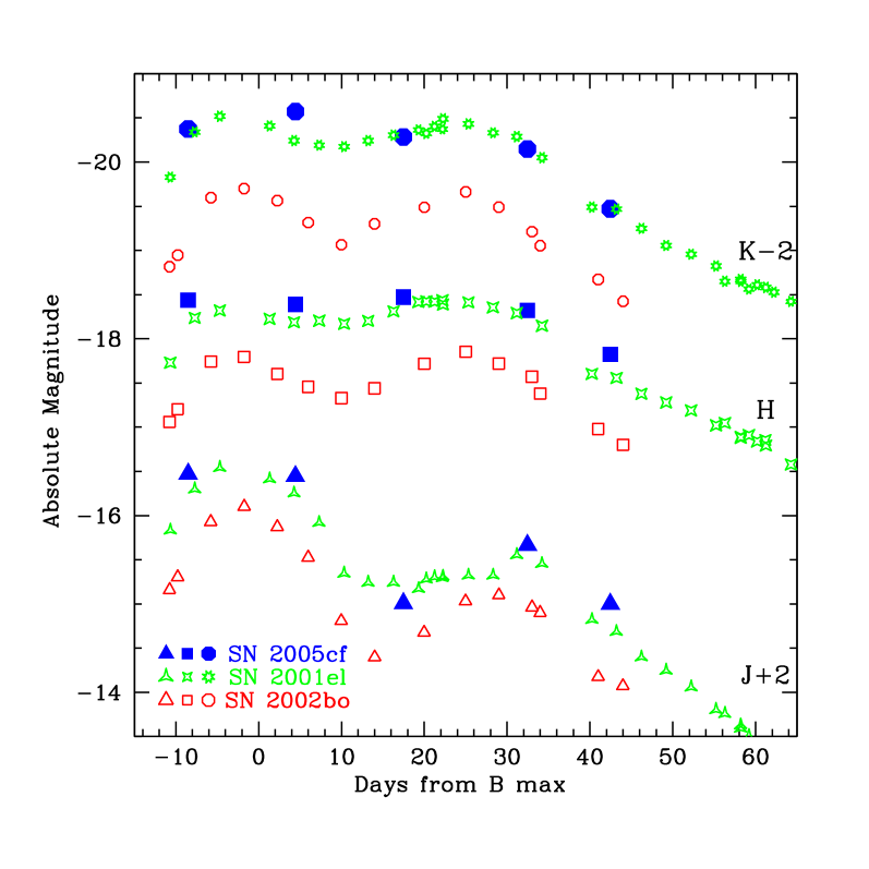
Figure 6: NIR absolute light curves of SNe 2005cf (blue filled symbols), 2001el (green starred symbols) and 2002bo (red open symbols). The sources of the data are cited in the text. $K^{\prime}$ photometry is displayed for SN 2005cf.

3.2 Near–IR Light Curves

Contrary to the optical photometry, no S–correction was applied to our NIR photometry, owing to the lack of adequate time coverage of the NIR spectroscopy. The NIR photometry available for SN 2005cf is shown in Tab. 7. In Fig. 6, the absolute NIR light curves of SN 2005cf are compared with those of the well–studied SNe 2001el (Krisciunas et al., 2003) and 2002bo (Krisciunas et al., 2004). The absolute magnitudes were computed assuming the distance modulus and total reddening values of Tab. 8 (see Sect. 3.4).

Table 7: $J$, $H$, $K^{\prime}$ magnitudes of SN 2005cf and assigned errors.

Date	JD	$J$	$H$	$K^{\prime}$	S
	(+2400000)
03/6	53525.49	14.13 (0.02)	14.13 (0.03)	14.17 (0.03)	A
16/6	53538.45	14.15 (0.03)	14.18 (0.03)	13.97 (0.03)	A
29/6	53551.48	15.59 (0.02)	14.10 (0.03)	14.26 (0.03)	B
14/7	53566.45	14.93 (0.02)	14.25 (0.03)	14.40 (0.03)	A
24/7	53576.47	15.60 (0.03)	14.75 (0.03)	15.07 (0.03)	A

A = Telescopio Nazionale Galileo 3.5m + NICS;
B = Calar Alto 3.5m Telescope + Omega–Cass

SN 2002bo is significantly fainter than both SN 2005cf and 2001el. However, we remark that the behaviour of SN 2002bo in the NIR is rather peculiar and that SN 2005cf was observed in the $K^{\prime}$ band, while SN 2001el and SN 2002bo were calibrated by Krisciunas et al., (2003, 2004) in the standard Persson’s system (Persson et al., 1998). The deep minimum in the $J$ band light curve of SN 2005cf resembles that observed in SN 2002bo, although the $J$ band luminosity is closer to that of SN 2001el. The plateau–like behaviour of the $H$ band light curve of SN 2005cf between phase about $-$10 and +30 is very similar to that observed in the light curve of SN 2001el. A strong similarity between SN 2005cf and SN 2001el is also seen in the $K$ band evolution. Their $K$ band light curves remain relatively flat from phase $-$10 and +30, while the maxima of SN 2002bo are somewhat more pronounced.

Recently, Kasen, (2006) explained the variable strength of the NIR secondary maximum in SNe Ia in terms of different abundance stratification, metallicities of the progenitor star and amounts iron–group elements synthesized in the explosion. In particular, Type Ia SNe ejecting more radioactive ⁵⁶Ni are expected to show, together with a brighter light curve, more pronounced NIR secondary maxima.

3.3 Reddening and Distance

SN 2005cf exploded very far from the nucleus of MCG –01–39–003, in a region with low background contamination. Deep late–time VLT imaging (F. Patat, private communication) shows that the SN exploded at the edge of a long tidal bridge connecting MCG –01–39–003 with the interacting companion (see also Vorontsov-Velyaminov & Arhipova, 1963), suggesting relatively small host galaxy interstellar extinction. This finding is supported by non–detection of narrow interstellar lines in the SN spectra. As Sect. 3.4 will show, a small value for the interstellar extinction is also supported by the normal colour curves of SN 2005cf. Therefore, in this paper we will adopt as total extinction the Galactic estimate at the coordinates of the SN, i.e. E$(B-V)$ = 0.097$\pm$0.010, reported by Schlegel et al., (1998).

Despite the relatively short distance, the galaxy system hosting SN 2005cf is poorly studied. As a consequence, large uncertainty exists in the distance estimate. For MCG –01–39–003 and NGC 5917 LEDA provides the recession velocities corrected for the effects of the Local Group infall onto the Virgo Cluster (208 km s^-1, Terry et al., 2002): v_Vir = 1977 and 1944 km s^-1 are reported for the two galaxies, respectively. However, we should take into account a non–negligible gravitational effect of the Virgo Cluster at the distance of the two galaxies. Taking into account the observed positions of the two galaxies relative to the Virgo centre, a crude estimate of the virgocentric component subtracts to the observed recession velocities about 3–400 km s^-1. hereafter we will adopt the first infall velocity model.

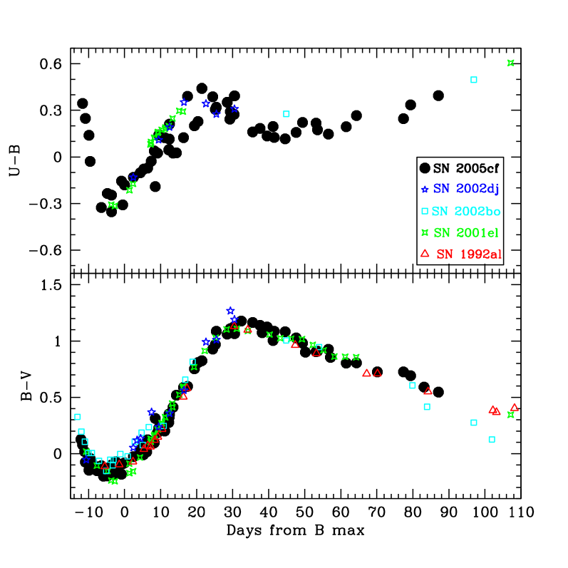
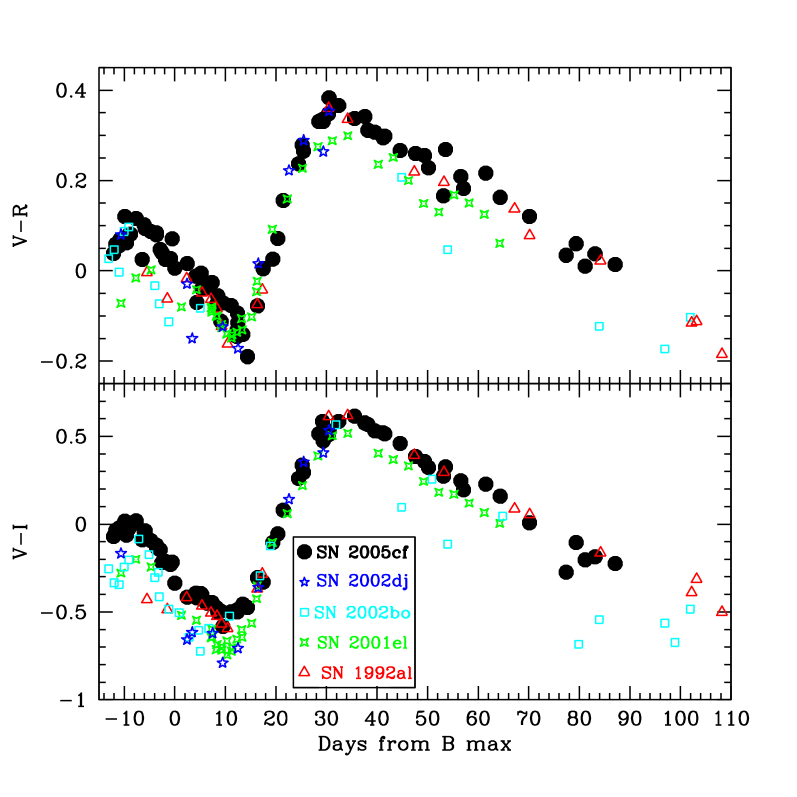
Figure 7: Colour evolution of SN 2005cf compared with other SNe Ia with similar $\Delta m_{15}(B)_{true}$: SNe 1992al, 2001el, 2002bo, 2002dj. Evolution of $U-B$ (top–left), $B-V$ (bottom–left), $V-R$ (top–right) and $V-I$ (bottom–right) colours. All colour curves are reddening corrected. For references, see the text.

Table 8: Basic information for the SNe Ia sample with $\Delta m_{15}(B)_{true}$ $\sim$1.1 included in this paper.

SN	host galaxy	$\mu$	E$(B-V)_{TOT}^{\otimes}$	JD$(B)_{max}$	$M_{B,max}$	$\Delta m_{15}(B)_{true}$	sources
2005cf	MCG –01–39–003	32.51	0.097	2453534.0	-19.39	1.12	1,0
2002dj	NGC 5018	32.92	0.15	2452450.5	-19.17	1.15	2,0
2002bo	NGC 3190	31.45	0.38	2452356.5	-18.98	1.17	3,4,0
2001el	NGC 1448	31.29	0.22‡	2452182.5	-19.35	1.13	5
1992al	ESO 234–G069	33.82	0.034	2448838.36	-19.37	1.11	6,0

^⊗ E(B-V)_Gal + E(B-V)_host; ^‡ E(B-V)_host = 0.18, with R_V = 2.88.
0 = LEDA; 1 = this paper; 2 = Pignata et al., in preparation; 3 = Benetti et al., (2004);
4 = Stehle et al., (2005); 5 = Krisciunas et al., (2003); 6 = Hamuy et al., (1996).

Kraan–Korteweg, (1986) computed distance estimates of a large sample of nearby galaxies based on a virgocentric non–linear flow model (see e.g. Silk, 1977). While MCG –01–39–003 and NGC 5917 are not listed in the catalogue, with a good approximation we can assume the same infall correction computed for another galaxy, NGC 5812, which projects very close to the SN 2005cf parent galaxy and has similar recession velocity (v_Vir = 1965 km $s^{-1}$, LEDA, cf. Tab. 1). In the Kraan–Korteveg’s catalogue, the distances are expressed in units of the Virgo Cluster distance (d_Vir). For NGC 5812 two alternative distances are derived from different assumptions on the virgocentric infall velocity of the Local Group: 1.91 d_Vir for a more commonly accepted 220 km s^-1 – model (Tammann & Sandage, 1985) or 1.84 d_Vir for a 440 km s^-1 – model (Kraan–Korteweg, 1986). Since a value for the local infall velocity toward Virgo of 220 km s^-1 is close to that currently adopted by LEDA (208 km s^-1),

To derive the distance modulus of SN 2005cf we need to adopt a distance for Virgo. For the latter, the values reported in the literature show some scatter. For instance, the mean Tully–Fisher distance of Virgo obtained by Fouqué et al., (2001) from 51 spiral galaxies members of the cluster is d = 18.0 $\pm$ 1.2 Mpc. This gives a distance of NGC 5812 of 34.4 Mpc ($\mu$ = 32.68).

Alternatively, computing the cepheid distances of 6 galaxies of the Virgo Cluster, Fouqué et al., (2001) found a somewhat smaller distance of Virgo: d = 15.4 $\pm$ 0.5 Mpc. The resulting distance of NGC 5812 is 29.4 Mpc ($\mu$ = 32.34). Averaging the distance moduli of NGC 5812 obtained from the two different estimates of the Virgo distance, we obtain $\mu$ = 32.51. We can reasonably adopt this distance modulus also for MCG –01–39–003 and NGC 5917. A conservative estimate of the error is obtained from the dispersion of the galaxy peculiar motions, i.e. $\sim$350 km s^-1 (Somerville et al., 1997), which gives a maximum error in the distance modulus of $\Delta$$\mu$ = 0.33. Hereafter, we will adopt $\mu$ = 32.51 $\pm$ 0.33 as our best distance modulus estimate for the galaxy hosting SN 2005cf.

3.4 Colour Curves, Absolute Luminosity and Bolometric Light Curve

In what follows, we compare colour evolution, absolute light curves and pseudo–bolometric luminosity of SN 2005cf with those of other Type Ia SNe with similar light curve shape. The range of $\Delta m_{15}(B)$ $\sim$ 1.0–1.2 (around the average value for normal SNe Ia) is well populated. As comparison objects we have selected SNe 1992al (Hamuy et al., 1996), 2001el (Krisciunas et al., 2003), 2002bo (Benetti et al., 2004; Krisciunas et al., 2004) and 2002dj (Pignata et al., in preparation). Basic information about the distance moduli and reddening values adopted for this sample is reported in Tab. 8. In particular, as already seen in Sect. 3.3, $\mu$ = 32.51 and E$(B-V)$ = 0.097 (Schlegel et al., 1998) were adopted for SN 2005cf.

In Fig. 7 the $U-B$ (top–left), $B-V$ (bottom–left), $V-R$ (top–right) and $V-I$ (bottom–right) intrinsic colour curves of SN 2005cf and the other similar SNe Ia mentioned above are shown. The colour evolution of all these objects is very similar, with a few minor differences. The $U-B$ colour (Fig. 7, top–left) has a steep decline (from 0.4 to about $-$0.3) until $\sim$4 days before maximum. Then the $U-B$ colour curves become redder, arriving at $\sim$0.3 about 3–4 weeks past maximum and being almost constant thereafter. SNe 2001el and 2002dj have a similar evolution.

The evolution of the $B-V$ colour curves (Fig. 7, bottom–left) is very similar for all SNe of our sample, showing a decreasing trend from $\sim$ 0.3 to $-$0.2 in the period 13 to 5 days before the $B$ band maximum. Then the $B-V$ colour rises for approximately one month, reaching a $B-V$ $\approx$ 1.2. In the subsequent two months, the $B-V$ colour becomes bluer again, to values below $\sim$0.5 at a phase of $\sim 90$ days past maximum.

The $V-R$ and $V-I$ colours show a similar behaviour (see Fig. 7, top–right and bottom–right). Soon after the explosion, the colours turn red. Then, between about a week before and two weeks past maximum, the trend is reversed (the $V-I$ colour, in particular, decreases from 0 to $-$0.7 in this time interval). Subsequently, until about 1 month past the $B$ band maximum, the colours become again redder ($V-R$ rises from $-$0.2 to +0.4, $V-I$ from $-$0.7 to 0.6), followed by a phase where they turn bluer again. About 3 months after maximum, the V–R colour reaches 0 and V–I about $-$0.3, with an ongoing trend to bluer values in the subsequent weeks. The only outlier is SN 2002bo, which seems to have bluer $V-R$ and $V-I$ colours at all phases, especially well after maximum.

A comparison of the absolute light curves of SN 2005cf and other similar events is shown in Fig. 8, both for the $B$ band (top panel) and the $I$ band (bottom panel). It is remarkable that the $I$ band secondary maximum, known to be more or less pronounced in different SNe Ia, is similarly prominent for the SNe of this sample. The $B$ band maximum magnitude of SN 2005cf is $M_{B,max}$ $\approx-$19.39, which is in the bright side of the SN Ia luminosity function. At the epoch of the $B$ band maximum, the dereddened colour is $(B-V)_{B,max}=-$0.09.

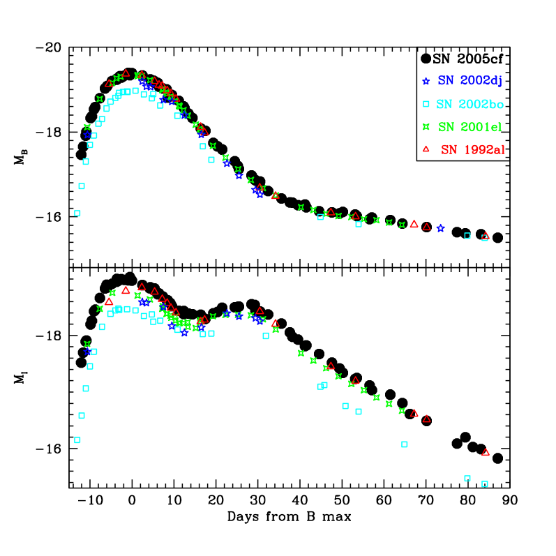
Figure 8: $B$ (top) and $I$ band (bottom) absolute light curves for SN 2005cf and other similar objects: SNe 1992al, 2001el, 2002bo, 2002dj. The values of $\mu$ and E$(B-V)$ adopted are shown in Tab. 8.

The luminosity evolution of SN 2005cf obtained integrating the fluxes in the optical bands is shown in Fig. 9. For comparison, also the observed pseudo–bolometric light curves for other similar SNe Ia are shown. Since $U$ band observations of SN 1992al are missing, we applied a $U$ band correction to its light curve following Contardo et al., (2000). The pseudo–bolometric light curves of our Type Ia SN sample are extremely similar, with the exception of SN 2002bo, which is fainter than SN 2005cf by a factor 0.75, suggesting a non–negligible scatter in luminosity also among similarly declining SNe Ia.

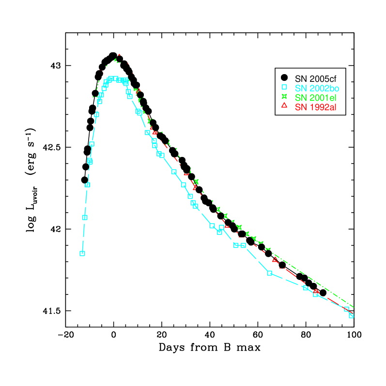
Figure 9: Quasi–bolometric light curves for SNe 2005cf, 1992al, 2001el and 2002bo. All these SNe Ia are characterised by similar values for the $\Delta m_{15}(B)$ parameter (about 1.1).

4 SN Parameters

The excellent photometric coverage of SN 2005cf allows us to precisely estimate the epoch, and the apparent and absolute magnitudes at the $B$, $V$ and $I$ maxima. The parameters for all bands are obtained by fitting the light curves with a low–degree spline function. The results are reported in Tab. 9. In particular, the epoch of the $B$ band maximum is found to be JD($B_{max}$) = 2453534.0$\pm$0.3 (June 12.5 UT).

Table 9: Parameters of SN 2005cf derived from the optical light curves. The errors in the absolute magnitudes are largely dominated by the uncertainty in the distance modulus estimate ($\pm$0.33). The values for A_λ are those provided by Schlegel et al., (1998).

	JD(max)	$m_{\lambda,max}$	Aλ	$M_{\lambda,max}$	$\Delta m_{15}(\lambda)_{obs}$
	(+24000000)
$U$	53532.4$\pm$0.6	13.40$\pm$0.05	0.53	$-$19.64	1.26 $\pm$ 0.05
$B$	53534.0$\pm$0.3	13.54$\pm$0.02	0.42	$-$19.39	1.11 $\pm$ 0.03
$V$	53535.3$\pm$0.3	13.53$\pm$0.02	0.32	$-$19.30	0.61 $\pm$ 0.02
$R$	53534.6$\pm$0.4	13.45$\pm$0.03	0.26	$-$19.32	0.71 $\pm$ 0.04
$I$	53532.0$\pm$0.5	13.70$\pm$0.03	0.19	$-$19.00	0.61 $\pm$ 0.06

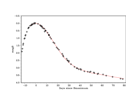
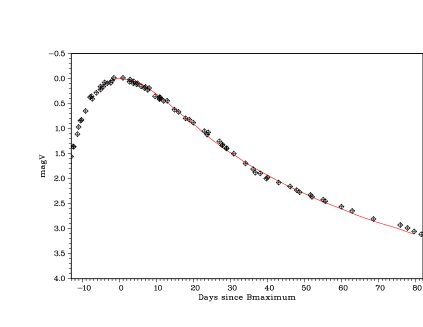
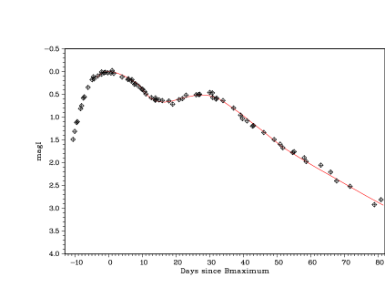
Figure 10: Comparison between light curves of SN 2005cf (diamonds) and the template SN 1992al (solid line, from Hamuy et al., 1996), in the $B$, $V$, $I$ bands (from top to bottom).

In Fig. 10 the B, V and I light curves of SN 2005cf are compared with those of the template SN 1992al (Hamuy et al., 1996). The match of the light curves is excellent and therefore one of the most important parameters for SNe Ia, the $\Delta m_{15}(B)$ is expected to be very similar. An observed $\Delta m_{15}(B)_{obs}$ $\approx$ 1.11 $\pm$ 0.03 is measured for SN 2005cf (see column 6 in Tab. 9), well matching that derived for SN 1992al (Hamuy et al., 1996). This value makes SN 2005cf a typical SN Ia. Owing to the low interstellar extinction suffered by SN 2005cf, the correction for reddening to apply to $\Delta m_{15}(B)$ is very small. The reddening corrected $\Delta m_{15}(B)_{true}$ is obtained applying the relation of Phillips et al., (1999):

$$\Delta m_{15}(B)_{true}=\Delta m_{15}(B)_{obs}+0.1\times E(B-V)$$ (2)

This gives $\Delta m_{15}(B)_{true}$ = 1.12.

An alternative parameter characterising the light curves of Type Ia SNe is the stretch factor s^-1 (Perlmutter et al., 1997), i.e. the coefficient indicating the stretch in time of the $B$ band light curve. We compute for SN 2005cf $s^{-1}$ = 0.99$\pm$0.02. This result is in excellent agreement with the value (0.995$\pm$0.179) derived applying the relation of Altavilla et al., (2004):

$$\Delta m_{15}(B)_{true}=1.98\times(s^{-1}-1)+1.13$$ (3)

The $\Delta m_{15}(B)$–calibrated absolute magnitude at the $B$ band maximum can be computed applying various relations available in literature. The relation between $M_{B,max}$ and $\Delta m_{15}(B)$ from Hamuy et al., (1996):

$$M_{\lambda,max}^{\star}=A+B\times[\Delta m_{15}(B)-1.1]$$ (4)

provides a preliminary tool to get a calibrated absolute magnitude at maximum for SN 2005cf. The label $M_{\lambda,max}^{\star}$ is to indicate that this magnitude has to be rescaled to H₀ = 72 km s^-1 Mpc^-1. Using the “low extinction case” parameters reported in Tab. 3 of Hamuy et al., (1996) and after rescaling $M_{B,max}^{\star}$ to H₀ = 72 km s^-1 Mpc^-1, we obtain $M_{B,max}$ =$-$19.03 $\pm$ 0.05. An updated, reddening–free decline rate vs. $\Delta m_{15}(B)$ relation was provided by Phillips et al., (1999) (see also their Tab. 3):

$$M_{\lambda,max}^{\star}=M_{\lambda,max}^{1.1}+a\times[\Delta m_{15}(B)-1.1]+b\times[\Delta m_{15}(B)-1.1]^{2}$$ (5)

From Eq. 5, using as $M_{\lambda,max}^{1.1}$ the coefficient A of Eq. 4 and reporting the magnitudes to H₀ = 72 km s^-1 Mpc^-1, we derive for SN 2005cf a reddening–corrected absolute magnitude of $M_{B,max}$ = 19.02$\pm$0.05. The magnitudes for the other bands can be found in Tab. 10.

Altavilla et al., (2004) used a further, updated version of Eq. 4, with different coefficients ($A$ = $-$19.403 $\pm$ 0.044 and $B$ = 1.061 $\pm$ 0.154, under the assumption of intermediate Cepheids metallicity, $\Delta$Y/$\Delta$Z = 2.5, and with R_B = 3.5). Applying the relation of Altavilla et al., we obtain $M_{B,max}$ = $-$19.35 $\pm$ 0.06 (for H₀ = 72 km s^-1 Mpc^-1).

Using a large sample of SNe Ia, Prieto et al., (2006) provided an updated version of the relation between absolute $B$ band magnitude at peak and post–maximum decline (Eq. 4, but with different values for the coefficients A and B). Using the coefficients of the low host galaxy extinction case (see Prieto et al., (2006), their Tab. 3, middle), we obtain for SN 2005cf $M_{B,max}$ = $-$19.31 $\pm$ 0.03. Estimates for other bands are reported in Tab. 10. The discrepancy of these magnitudes with those derived from other methods (see Tab. 10) may be due to the uncertainty in the zeropoints of the Eq. 4 reported in Prieto et al., (2006). Using different sub–samples, the scatter in the zeropoint values is between 0.10 and 0.15 magnitudes in all bands (see their Tab. 4).

Another approach for estimating the absolute magnitude at maximum is that of Reindl et al., (2005), who computed the value from $\Delta m_{15}(B)$ and colour at maximum. Rewriting their Eq. (23),

$$M_{\lambda,max}^{\star}=\alpha\times[\Delta m_{15}(B)-1.1]+\beta\times[(B-V)_{0}+0.024]+\gamma$$ (6)

with the coefficients $\alpha$, $\beta$ and $\gamma$ reported in Tab. 5 of Reindl et al., (2005), and with $(B-V)_{0}$ obtained from their empirical relation

$$(B-V)_{0}=0.045\times\Delta m_{15}(B)-0.073$$ (7)

we obtain the absolute magnitudes shown in Tab. 10. For the $B$ band it is $-$19.16 $\pm$ 0.06 (with H₀ = 72 km s^-1 Mpc^-1).

Table 10: $\Delta m_{15}(B)$–corrected absolute magnitudes for SN 2005cf. All absolute magnitudes are scaled to H₀ = 72 km s^-1 Mpc^-1.

method	$M_{B,max}$	$M_{V,max}$	$M_{I,max}$
Phillips et al. (1999)‡	$-$19.02$\pm$0.05	$-$19.03$\pm$0.05	$-$18.76$\pm$0.05
Altavilla et al. (2004)	$-$19.35$\pm$0.06
Prieto et al. (2006)	$-$19.31$\pm$0.03	$-$19.24$\pm$0.03	$-$18.97$\pm$0.03
Reindl et al. (2005)	$-$19.16$\pm$0.06	$-$19.14$\pm$0.04	$-$18.89$\pm$0.07
Wang et al. (2005)	$-$19.27$\pm$0.09	$-$19.20$\pm$0.09	$-$18.86$\pm$0.09
Average Values	$-$19.28$\pm$0.08	$-$19.20$\pm$0.05	$-$18.90$\pm$0.06
Distance (Tab. 9)	$-$19.39$\pm$0.33	$-$19.30$\pm$0.33	$-$19.00$\pm$0.33

^‡ Not considered in the computation of the average absolute magnitudes

An alternative method was recently proposed by Wang et al., (2005), who introduced a new parameter, the intrinsic B–V colour 12 days after maximum light ($\Delta C_{12}$), which is correlated with the absolute magnitude via the empirical formula:

$$M_{\lambda,max}=M_{0}+R\times\Delta C_{12}$$ (8)

where the parameter $\Delta C_{12}$ is found to be 0.354 $\pm$ 0.022 using $\Delta m_{15}(B)$ = 1.12 and the relation of Wang et al.:

$$\Delta C_{12}=0.347+0.401\times D_{15}^{B}-0.875\times(D_{15}^{B})^{2}+2.44\times(D_{15}^{B})^{3}$$ (9)

where $D_{15}^{B}$ = $\Delta m_{15}(B)$ – 1.1. The values of the parameters $M_{0}$ and $R$ are reported in Tab. 2 of Wang et al., (2005). This provides $M_{B,max}$ = $-$19.27 $\pm$ 0.09. Estimates for the $V$ and $I$ band are also reported in Tab. 10.

Averaging the calibrated absolute magnitudes obtained applying different methods (those obtained with the older relations of Phillips et al., (1999) were not considered), the following estimates have been obtained for SN 2005cf: $M_{B,max}$ = $-$19.28$\pm$0.08, $M_{V,max}$ = $-$19.20$\pm$0.05 and $M_{I,max}$ = $-$18.90$\pm$0.06, where the errors are the standard deviations of the available estimates (see Tab. 10). From the average absolute peak magnitudes, we obtain the following reddening–corrected colours: $B-V$ = $-$0.08 and $V-I$ = $-$0.30, which are well consistent with those obtained from the direct measurements in Tab. 9, being $-$0.09 and $-$0.30 respectively.

Another interesting parameter is the rise time $t_{r}$ in the $B$ band, i.e. the time spent by the SN from the explosion to the $B$ band maximum. A first attempt to estimate this parameter was performed by Pskovskii, (1984), who found it to be related to the post–maximum decay rate $\beta$, closely related to the $\Delta m_{15}(B)$, via the relation:

$$t_{r}=13+0.7\beta$$ (10)

For SN 2005cf $\beta$ is estimated to be about 7.47 mag/100^d, setting the explosion epoch $t_{r}\sim$ 18.2 days before the $B$ band maximum. Another more recent method was suggested by Riess et al., 1999b . In a first approximation, very young SNe Ia are homologously expanding fireballs, where the luminosity is proportional to the square of time since explosion. Riess et al., 1999b derived $t_{r}$ from the relation:

$$L(t)=A\times(t+t_{r})^{2}$$ (11)

where $t$ is the elapsed time relative to the maximum and $A$ is a parameter describing the raising rate. Using very early photometric data in the $R$ band (including the earliest unfiltered measurements from IAU Circ. 8535, and considering data until $\sim$9 days before maximum), we find that SN 2005cf exploded 19.2 days before the $R$ band maximum (JD = 2453515.4). This corresponds to a rise time to maximum in the $B$ band $t_{r}$ $\approx$ 18.6$\pm$0.4 days, not far from that derived applying Eq. 10, but slightly shorter than the 19.5$\pm$0.2 days found by Riess et al., 1999b for an object with $\Delta m_{15}(B)\approx$ 1.1. However, the value of $t_{r}$ obtained for SN 2005cf is in good agreement with that derived by Benetti et al., (2004) for the similar declining SN 2002bo ($t_{r}$ = 17.9$\pm$0.5).

5 Light curve models and ⁵⁶Ni Mass Estimate

An useful tool to estimate the properties of a SN is the modelling of its bolometric light curve. The bolometric light curves of our SN sample were computed applying the UV and NIR corrections from Suntzeff, (1996) to the observed quasi–bolometric light curves of Fig. 9. The bolometric light curves of SNe 2005cf, 1992al and 2001el are identical, while that of SN 2002bo is fainter (see also Fig. 9 for a comparison). In Fig. 11 the bolometric light curves of SNe 2005cf and 2002bo (those of SNe 1992al and 2001el are not shown) are compared with the models described below. The masses of the different components of the ejecta adopted in the models are reported in Tab. 11.

Figure 11: Comparison between the observed bolometric light curves of SNe 2005cf (circles) and 2002bo (triangles), and the bolometric light curve models obtained using the W7 density distribution and the abundances derived from the spectral analysis of Stehle et al. (2005). The dotted curve is a W7–based model with 0.7M_⊙ of ⁵⁶Ni. The two solid curves are a models obtained starting from Ni08-10$\%$ but increasing the NSE abundances at high velocities as in Stehle et al. (2005): the thin lower curve is the model used for SN 2002bo, while the thick higher is the model rescaled to the luminosity of SN 2005cf.

We used a gray Monte Carlo light curve code (Mazzali et al., 2001) to reproduce the bolometric light curve and derive the properties of the ejecta. The code computes the transport of the $\gamma$–rays and the positrons emitted by the decay ⁵⁶Ni $\rightarrow$ ⁵⁶Co $\rightarrow$ ⁵⁶Fe, and then the transport of the optical photons generated by the deposition of the energy carried by the $\gamma$–rays and the positrons in the expanding SN ejecta. We assume that the ejecta mass is 1.4M_⊙, and that the density–velocity distribution is described by the W7 model (Nomoto et al., 1984). Compared to a model with 0.7M_⊙ derived with the W7 density and abundance distributions (dotted curve in Fig.11), the light curve of SN 2005cf ($\Delta m_{15}(B)$ = 1.12, $\Delta m_{15}(V)$ $\sim$ 0.6, $\Delta m_{15}(Bol)$ $\approx$ 0.9) is broader.

A factor that could make a light curve broad for its luminosity is the relative content of (⁵⁸Ni+⁵⁴Fe) / ⁵⁶Ni (Mazzali & Podsiadlowski, 2006). For the same total mass of material in nuclear statistical equilibrium (NSE), a higher (⁵⁸Ni+⁵⁴Fe) / ⁵⁶Ni ratio produces a dimmer light curve that has a comparable width. We find that the light curve of SN 2005cf is better fitted by models where the ratio is larger than in W7. In particular, in order to match the bolometric light curve of SN 2005cf, we start from a model where the ⁵⁶Ni mass is intially rescaled to 0.8M_⊙, but then 10$\%$ of ⁵⁶Ni is replaced with non–radioactive ⁵⁸Ni and ⁵⁴Fe (model Ni08–10$\%$, see Mazzali & Podsiadlowski, (2006)). Such a high ratio of stable versus radioactive Fe–group elements ($\sim$50$\%$) is unlikely for W7–like ignition conditions, but is not excluded for higher ignition densities and/or higher–than–solar metallicities (Roepke at al., 2006).

Table 11: Parameters adopter in the light curve models shown in Fig. 11.

Model	ID curve	M(56Ni)	M(58Ni+54Fe)	M(IME+CO)
Ni07	dotted	0.7M⊙	0.3M⊙	0.4M⊙
Ni08–10$\%$	${\ddagger}$	0.72M⊙	0.38M⊙	0.3M⊙
SN 2002bo	lower solid	0.52M⊙	0.36M⊙	0.5M⊙
SN 2005cf	higher solid	0.7M⊙	0.4M⊙	0.3M⊙

${\ddagger}$ This model (see Mazzali & Podsiadlowski, 2006) is not shown in Fig. 11

The model described above (not shown in Fig. 11) has M(⁵⁶Ni) $\sim$ 0.72M_⊙ and total M(NSE) $\sim$ 1.1M_⊙ (see Tab. 11), but produces a luminosity peak that is too bright. In the case of SN 2002bo, the fast rise of the light curve could be reproduced adopting the ⁵⁶Ni distribution derived from fitting a time sequence of spectra (Stehle et al., 2005, Fig. 11, thin lower solid curve). That distribution reached higher velocities than W7. In that model, M(⁵⁶Ni) $\sim$ 0.52M_⊙ and M(NSE) $\sim$ 0.9M_⊙ were adopted. Now we rescale our Ni08–10$\%$ model to the abundance distribution of the model used to fit SN 2002bo, although we cannot justify this with spectroscopic results. The resulting model, with M(⁵⁶Ni) $\sim$ 0.7M_⊙ and a mass of NSE elements of about 1.1M_⊙, fits the light curve of SN 2005cf quite well (Fig. 11, thick higher solid curve). In total, 1.1M_⊙ are burned to NSE, and only 0.3M_⊙ are intermediate–mass elements (IME) or unburned material (CO). Similar values, in particolar an ejected ⁵⁶Ni mass of about 0.7M_⊙, are also obtained for SNe 1992al and 2001el. Spectroscopic models will be necessary to refine these estimates.

6 Summary

Extensive optical photometric observations of the nearby Type Ia SN 2005cf obtained by the ESC are presented. The observations span a period of about 100 days, from $-$12 until +87 days from the $B$ band maximum.

Being a standard, normally–declining SN Ia, with a reddening corrected $\Delta m_{15}(B)$ = 1.12, its light curves well match those of SNe 1992al and 2001el in optical bands. SN 2005cf can be considered a good template, having been discovered a short time after the explosion and being densely sampled. Despite some uncertainty in the distance of the host galaxy, its absolute magnitude at maximum (M${}_{B}=-$19.39$\pm$0.33) is close to those of SNe 1992al and 2001el, but SN 2005cf is probably intrinsically brighter than the similarly–declining SN 2002bo. The colour evolution of SNe Ia in the $\Delta m_{15}(B)$ range 1.1–1.2 appears to be rather homogeneous.

The rise time of SN 2005cf to the $B$ band maximum is computed to be 18.6$\pm$0.4 days, slightly shorter than expected for a SN with such $\Delta m_{15}(B)$.

Finally, the bolometric light curve modelling indicates an ejected ⁵⁶Ni mass of about 0.7M_⊙, which is close to the average value of the ⁵⁶Ni mass distribution observed in normal SNe Ia (0.4–1.1 M_⊙, Cappellaro et al., 1997).

Spectroscopic data that will be presented in a forthcoming paper (Garavini et al., 2007) will provide further information about the properties of this normal object, and the degree of homogeneity among the mid–declining SNe Ia.

References

- Altavilla et al., (2004) Altavilla, G. et al., 2004, MNRAS, 349, 1344
- Astier et al., (2006) Astier, P., et al, 2006 A&A, 447, 31
- Benetti et al., (2004) Benetti, S. et al., 2004, MNRAS, 348, 261
- Benetti et al., (2005) Benetti, S. et al., 2005, ApJ, 623, 1011
- Bessell, (1990) Bessell, M. S., 1990, PASP, 102, 1181
- Cappellaro et al., (1997) Cappellaro, E., Mazzali, P. A., Benetti, S., Danziger, I. J., Turatto, M., della Valle, M., 1997, A&A, 328, 203
- Conley et al., (2006) Conley, A., et al., 2006, AJ, 132, 1707
- Contardo et al., (2000) Contardo, G., Leibundgut, B., Vacca, W. D., 2000, A&A, 359, 876
- Della Valle & Livio, (1994) Della Valle, M., Livio, M., 1994, ApJ, 423, L31
- Della Valle et al., (2005) Della Valle, M., Panagia, N., Padovani, P., Cappellaro, E., Mannucci, F., Turatto, M., 2005, ApJ, 629, 750
- Elias–Rosa et al., (2006) Elias-Rosa, N. et al., 2006, MNRAS, 369, 1880
- Fouqué et al., (2001) Fouqué, P., Solanes, J. M., Sanchis, T., Balkowski, C., 2001, A&A, 375, 770
- Garavini et al., (2007) Garavini, G. et al., 2007, AA, in press
- Hamuy et al., (1994) Hamuy, M., Suntzeff, N. B., Heathcote, S. R., Walker, A. R., Gigoux, P., Phillips, M. M., 1994, PASP, 106, 566
- Hamuy et al., (1996) Hamuy, M. et al., 1996, AJ, 112, 2408
- Hachinger et al., (2006) Hachinger, S., Mazzali, P. A., Benetti, S., 2006, MNRAS, 370, 299
- Hopp & Fernàndez, (2002) Hopp, U., Fernàndez, M., 2002, International Report 17/10/2002
- Hunt et al., (1998) Hunt, L. K., Mannucci, F., Testi, L., Migliorini, S., Stanga, R. M., Baffa, C., Lisi, F., Vanzi, L., 1998, AJ, 115, 2594
- Jha et al., (2006) Jha, S. et al., 2006, AJ, 131, 527
- Kasen, (2006) Kasen, D., 2006, ApJ, 649, 939
- King, (1985) King, D. L., 1985, RGO/La Palma technical note No. 31
- Kotak et al., (2005) Kotak, R. et al., 2005, AA, 436, 1021
- Kraan–Korteweg, (1986) Kraan–Korteweg, R. C., 1986, A&AS, 66, 255
- Krisciunas et al., (2003) Krisciunas, K., et al., 2003, AJ, 125, 166
- Krisciunas et al., (2004) Krisciunas, K., et al., 2004, AJ, 128, 3034
- Landolt, (1992) Landolt, A. U., 1992, AJ, 104, 340
- Mazzali et al., (2001) Mazzali, P. A., Nomoto, K., Cappellaro, E., Nakamura, T., Umeda, H., Iwamoto, K., 2001, ApJ, 547, 988
- Mazzali et al., (2005) Mazzali, P. A. et al., 2005, ApJ, 623, 37
- Mazzali & Podsiadlowski, (2006) Mazzali, P. A., Podsiadlowski, Ph., 2006, MNRAS, 369L, 19
- Modjaz et al., (2005) Modjaz, M., Kirshner, R., Challis, P., Berlind, P. 2005, IAU Circ. 8534, 3
- Navasardyan et al., (2001) Navasardyan, H., Petrosian, A. R., Turatto, M., Cappellaro, E., Boulesteix, J., 2001, MNRAS, 328, 1181
- Nomoto et al., (1984) Nomoto, K., Thielemann, F.-K., Yokoi, K., 1984, ApJ, 286, 644
- Pastorello et al., (2007) Pastorello, A. et al., 2007, MNRAS, submitted
- Perlmutter et al., (1997) Perlmutter, S.. et al., 1997, ApJ, 483, 565
- Persson et al., (1998) Persson, S. E. et al., 1998, AJ, 116, 2475
- Petrosian & Turatto, (1995) Petrosian, A. R., Turatto, M., 1995, A&A, 297, 49
- Phillips et al., (1993) Phillips, M. M., 1993, ApJ, 413, L105
- Phillips et al., (1999) Phillips, M. M., Lira, P., Suntzeff, N. B., Schommer, R. A., Hamuy, M., Maza, J. 1999, AJ, 118, 1766
- Pignata et al., (2004) Pignata, G. et al., 2004, MNRAS, 355, 178
- Prieto et al., (2006) Prieto, J. L., Rest, A., Suntzeff, N. B., 2006, ApJ, 647, 501
- Pskovskii, (1984) Pskovskii, Yu. P., 1984, Soviet Astron., 28, 658
- Puckett et al., (2005) Puckett, T., Langoussis, A., Chen, Y.-T., Hu, C.-P., Pugh, H., Li, W., Harris, B. 2005, IAU Circ. 8534, 1
- Reindl et al., (2005) Reindl, B., Tammann, G. A., Sandage, A., Saha, A., 2005, ApJ, 624, 532
- (44) Riess, A. G. et al., 1999a, AJ, 117, 707
- (45) Riess, A. G. et al., 1999b, AJ, 118, 2675
- Roepke at al., (2006) Roepke, F. K., Gieseler, M., Reinecke, M., Travaglio, C., Hillebrandt, W., 2006, A&A, 453, 203
- Schlegel et al., (1998) Schlegel, D. J., Finkbeiner, D. P., Davis, M. 1998, ApJ, 500, 525
- Silk, (1977) Silk, J., 1977, A&A, 59, 53
- Smirnov & Tsvetkov, (1981) Smirnov, M. A., Tsvetkov, D. Yu., 1981, Pis’ma Astr. Zh., 7, 154
- Somerville et al., (1997) Somerville, R. S., Davis, M., Primack, J. R., 1997, ApJ, 479, 616
- Stanishev et al., (2007) Stanishev, V., et al., 2007, A&A, submitted
- Stehle et al., (2005) Stehle, M., Mazzali, P. A., Benetti, S., Hillebrandt, W., 2005, 360, 1231
- Stritzinger et al., (2002) Stritzinger, M. et al., 2002, AJ, 124, 2100
- Stritzinger et al., (2005) Stritzinger, M., Suntzeff, N. B., Hamuy, M., Challis, P., Demarco, R., Germany, L., Soderberg, A. M., 2005, PASP, 117, 810
- Suntzeff, (1996) Suntzeff, N. B., 1996 in McCray R., Wang Z. eds, Proc. IAU Colloquium 145, Supernovae and Supernova Remnants, Cambridge: University Press, P. 41
- Tammann & Sandage, (1985) Tammann, G. A., Sandage, A., 1985, ApJ, 294, 81
- Terry et al., (2002) Terry, J. N., Paturel, G., Ekholm, T., 2002, A&A, 393, 57
- Vorontsov-Velyaminov & Arhipova, (1963) Vorontsov-Velyaminov, B., Arhipova, V. P. 1963 ”Morphological Catalogue of Galaxies”, Vol. 3, Moscow State University
- Walker, (1987) Walker, G., 1987, Astronomical Observations. Cambridge Univ. Press, Cambridge, p. 47
- Wang et al., (2005) Wang, X., Wang, L., Zhou, X., Lou, Y.-Q. Li, Z., 2005, ApJ, 620L, 87