The size and structure of the spheroid of IC 1613

Abstract

Context. Nearby galaxies, spirals as well as irregulars, have been found to be much larger than previously believed. The structure of the huge spheroid surrounding dwarf galaxies could give clues to their past gravitational history. Thanks to wide field imagers, nearby galaxies with diameter of dozens of arcmin can be effectively surveyed.

Aims. We obtain, from the CFHT archives, a series of $i^{\prime}$ and $g^{\prime}$ MegaCam images of IC 1613 in order to determine the stellar surface density of the field and determine the shape of its spheroid.

Methods. From the colour magnitude diagram we select some 36,000 stars, in the first three magnitudes of the red giant branch. The spatial distribution of these stars is used to establish the structure of the spheroid.

Results. The position angle of the major axis of the stellar spheroid is found to be $\approx 90^{\circ}$, some 30^∘ from the major axis of the HI cloud surrounding IC 1613. The surface density profile of the spheroid is not exponential over all the length of the major axis. A King profile, with a core radius of 4.5^′ and a tidal radius of 24^′ fits the data. The tidal truncation of the spheroid suggests that IC 1613 is indeed a satellite of M31.

1 Introduction

In recent years surveys of outer regions of nearby galaxies have revealed that galaxies are surprisingly large. Suffice to mention of few examples: the disk of NGC 300 has been detected to up to 10 scale lengths (Bland-Hawthorn et al. 2005); stars belonging to M31 are found up to a distance of 165 kpc (Kalirai et al. 2006); while for dwarf irregular galaxies, Battinelli et al. (2006) mapped the spheroid of NGC 6822 to 36^′ making it as big as the SMC. The less luminous dwarf, Leo A was also found to possess a huge halo/spheroid, (Vansevičius et al. 2004). For even less massive systems, McConnachie & Irwin (2006b) have demonstrated that the dwarf spheroidals, satellites of M31, are generally larger than previously recognized.

The recent advance in wide field imaging allows the survey of nearby galaxies with angular diameters reaching nearly one degree. Such survey provides information on the individual halo structure and permits the determination of universal parameters related to the morphology. With this in mind, we have selected one of the bright dwarf irregular galaxies of the Local Group.

Luminosity wise, with M_v = –14.9, IC 1613 ranks 6^th among the 15 dwarf irregular (dIrr) galaxies of the Local Group, being between NGC 3109 and Sextans A. Its distance has been accurately determined by Dolphin et al. (2001), from the apparent magnitude of the red giant branch tip (TRGB) and the red clump stars, who obtained $\mu_{o}$ = 24.31 $\pm$ 0.06 or 730 $\pm$ 20 kpc. Pietrzyński et al. (2006) determined its distance to be $\mu_{o}$ = 24.291 $\pm$ 0.014, from near infrared photometry of its Cepheids. Based on these two estimates, we adopt 722 $\pm$ 5 kpc for the distance of IC 1613. Its global structure has been investigated by Hodge et al. (1991) using UK Schmidt plates scanned with COSMOS. They follow the radial stellar density profile to 400^′′. They were, however, unable to decide if an exponential profile, with a scale length of 800 pc or a King model with a core radius of 200 $\pm$ 50^′′ and a tidal radius of 1420 $\pm$ 25^′′ give a better representation of the profile. The major axis diameter of IC 1613 is given by NED/IPAC to be 16.2^′. This diameter appears small on the light of the carbon star survey by Albert et al. (2000) who identified some 200 C stars extending to 15^′, essentially doubling the size of IC 1613. Tikhonov & Galozutdinova (2002) later mapped the surface density of giants ($8^{\prime}<r<12^{\prime}$) and concluded that the density variation follows and exponential and that they have not reached the limit.

The HI density and velocity maps of IC 1613 were analyzed by Lake & Skillman (1989). They conclude that the rotation curve of IC 1613 shows evidences for dark matter in the outer parts. They established that the position angle of the major axis is 58 $\pm 4^{\circ}$. A survey to fainter limits by Hoffman et al. (1996) reach a maximum diameter of $54^{\prime}$. Since Hodge et al. (1991) optical survey barely reached 7^′ from the center, it is certainly warranted to survey a larger area to establish which surface density profile best fits the data.

2 Photometric data

We use for our survey five $i^{\prime}$ and five $g^{\prime}$ archival CFHT Megacam images. The wide field imager MegaCam consists of 36 2048 $\times$ 4612 pixel CCDs, covering nearly a full 1${}^{\circ}\times 1^{\circ}$ field. It is mounted at the prime focus of the 3.66 m Canada-France-Hawaii Telescope. It offers a resolution of 0.187 arc second per pixel. These filters are designed to match Sloan Digital Sky Survey (SDSS) filters, as defined by the Smith et al. (2002) standards. The exposure times were, respectively 205 s and 135 s. Ten consecutive exposures were taken, essentially all with the same airmass.

The images secured from the CFHT archives were already processed and calibrated by Elixir (Magnier & Cuillandre 2004). The Elixir system performs a pre-reduction of the Megacam mosaic to produce calibrated flat-fielded, fringe-corrected images ready for further processing. In order to obtain a uniform zero point across the mosaic, all 36 CCDs are converted to a similar gain times quantum efficiency. This is easily achieved by dividing the mosaic image by a flat-fielded Mosaic which CCDs have been normalized with respect to CCD00 to maintain the ratio of gain and quantum efficiency. The result of the division is a flat looking image. Magnier & Cuillandre (2004) quote a formal scatter of magnitude residuals, across the mosaic of 0.0086 mag.

These images, obtained in Queue observing mode, are provided with calibration equations. However, since the calibration includes colour terms which are function of ($g^{\prime}-r^{\prime}$) or ($r^{\prime}-i^{\prime}$) we cannot fully calibrate our data because there is no $r^{\prime}$ observations avavilable for IC 1613. No aperture correction has been applied to the derived photometry. Taking into account the exposure times and the airmasses, the calibration equations given in the headers can be expressed as:

$$g^{\prime}=g^{\prime}_{inst}+6.781+0.15(g^{\prime}-r^{\prime}),$$

$$i^{\prime}=i^{\prime}_{inst}+6.520+0.08(r^{\prime}-i^{\prime}),$$

where the instrumental magnitudes refer to those calculated by DAOPHOT. The exposure times are sufficiently short that we have acquired only the first few magnitudes of the stellar population of IC 1613, as we shall display in the next Section. Since most stars are on the red giant branch (RGB), with ($g^{\prime}-r^{\prime})\approx$ 1.3, while 0.6 $<$ $(r^{\prime}-i^{\prime})$ $<$ 1.6, the $g^{\prime}$ colour term may be as large as 0.2 mag, or even larger for carbon stars which have extreme $(g^{\prime}-r^{\prime})$ colours; while the $i^{\prime}$ colour term may reach 0.13 mag. The exact magnitude and colour are not essential for our goals. For the moment we simply neglect the colour terms and take into account only the magnitude zero points.

2.1 Data analysis

Before precessing the images with DAOPHOT we astrometrically combine the five exposures of each filter into one $g^{\prime}$ and $i^{\prime}$ image for each of the 36 CCDs of the MegaCam mosaic. The DAOPHOT-II/ALLSTAR package (Stetson 1987, 1994) is selected to process each CCD image. Thresholds are adopted, employing Stetson’s procedure. Final instrumental magnitudes are obtained with ALLSTAR which fits a model PSF to all stellar objects on the frame. Figure 1 displays the photometric errors, as defined by ALLSTAR, as a function of the $i^{\prime}$ magnitudes for one CCD which includes IC 1613.

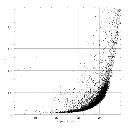
Figure 1: The photometric error, as determined by ALLSTAR, for a CCD which includes IC 1613. To reduce the colour scatter we exclude objects with magnitude error, both in $i^{\prime}$ and $g^{\prime}$, less than 0.15.

In order to exclude objects with large colour errors we select, before combining the $i^{\prime}$ and $g^{\prime}$ magnitude files, only stars with photometric errors (as defined by ALLSTAR) less than 0.15 mag. This results in a total of 85809 objects in one square degree. Because IC 1613 is located at a Galactic latitude of b = $-61^{\circ}$, an impressive number of galaxies is seen in the surrounding field. Therefore, to reduce the background counts these non-stellar objects should be eliminated. DAOPHOT-II provides an image quality diagnostics SHARP that can be used to separate stellar and non-stellar objects. For isolated stars, SHARP should have a value close to zero, whereas for semi-resolved galaxies and unrecognized blended doubles SHARP will be significantly greater than zero. On the other end, bad pixels and cosmic rays produce SHARP less than zero. SHARP must be interpreted as a function of the apparent magnitude of all objects because the SHARP parameter distribution flares up near the magnitude limit; see Stetson & Harris (1988) for a discussion of this parameter.

Figure 2 shows the SHARP distributions, as a function of the apparent magnitude, for two CCDs inside and two CCDs outside of IC 1613. The dashed line, at 16.80 mag, indicates the saturation limit. We see a large population of non-stellar objects well above the limiting magnitude of the sample. Indeed, visual inspection of several $i^{\prime}$ and $g^{\prime}$ images reveals that bright objects with larger SHARP have larger than normal FWHM while fainter ones are obviously non-stellar. Based on this figure, we exclude objects with $|$SHARP$|$ $>$ 0.5 from our stellar database. There are 63000 stars satisfying the magnitude and SHARP criteria, their spatial distribution, in the one squared degree area, is presented in Figure 3. The gaps between the Megacam CCDs are evident. Bright foreground stars are responsible for the small regions lacking stars. Just North-East of IC 1613 the empty spot is due to an 8th magnitude star.

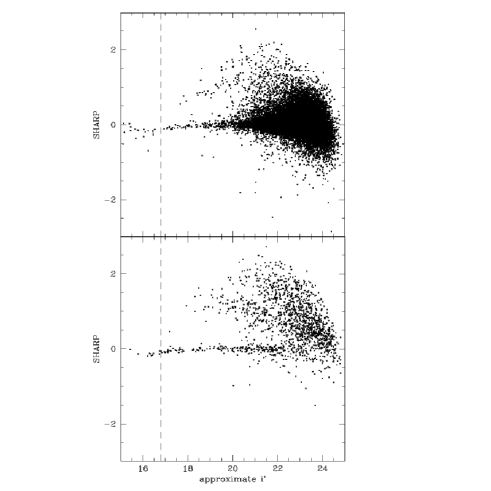
Figure 2: Distributions of the SHARP parameter for objects with photometric error $<$ 0.15 mag. The upper panel corresponds to two CCDs within IC 1613 while the bottom panel is for two CCDs outside the galaxy. We see a huge population of non-stellar objects brighter that the magnitude limit. Close to the magnitude limit, SHARP becomes meaningless due to the large scatter. The dashed line marks the saturation threshold.

2.2 Completeness tests

In order to establish the efficiency of DAOPHOT/ALLSTAR to recover faint stars among the various stellar density encountered, we perform a series of completeness tests. For a given CCD of the mosaic, the test consists in the addition of 140 stars, uniformly distributed in magnitude between $i^{\prime}$ = 20.0 and 24.6 and with corresponding $g^{\prime}$ magnitudes that match giant branch stars of IC 1613. The stars are added to the $i^{\prime}$ and $g^{\prime}$ images, they are then analyzed with DAOPHOT/ALLSTAR, the results are combined to produce a list of stars with magnitudes and colours, thus only stars with recovered $i^{\prime}$ and $g^{\prime}$ are counted. As representative of different crowding conditions over the field, we selected 2 in the center, 2 in the periphery and 2 outside the galaxy. For each CCD we performed 6 tests with a total of 980 added stars. We find that, except for the two central CCDs where the density is highest, the completeness is 75% at $i^{\prime}$ = 24.0 and drops to 50% and 24.6. The completeness of the two central CCDs at $i^{\prime}$ = 24.0 is 50%. However, because of the strong radial gradient of the surface density, the completeness in the inner halves of the central CCDs is even lower while in the outer halves we find completeness levels ($\sim$80%) similar to those found for the periphery. For the above reasons, we will exclude the inner 5^′ from any further interpretation of the data. In the following analysis we restrict our counts to stars brighter than $i^{\prime}$ = 24.0.

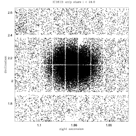
Figure 3: Spatial distribution of all stars with $i^{\prime}$ $<$ 24.0 and selected following the SHARP criterion described above.

3 Results

3.1 Space distribution of young and old populations

Figure 4 presents the colour-magnitude diagram of the whole $1^{\circ}\times 1^{\circ}$ field. Only stars with error and SHARP satisfying the adopted criteria are plotted. A well-defined giant branch is seen, along with main sequence stars and an extended AGB where known C stars are located. According to Dolphin et al. (2001), the TRGB of IC 1613 is seen at I = 20.35 $\pm 0.07$. On Fig. 4 we see that the number of stars per magnitude interval nearly double between $i^{\prime}$ = 20.80 and 20.90. This is essentially consistent with the quoted TRGB since the difference between the $i^{\prime}$ and I magnitudes in the colour range of the TRGB is $\sim$0.60 mag (Battinelli et al. 2006).

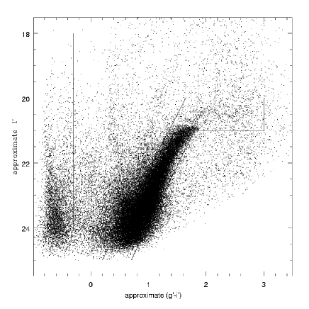
Figure 4: Colour-magnitude diagram of the whole field, 63,000 objects satisfying the error and SHARP criteria, are plotted. The giant box encloses the RGB and AGB stars, while the blue stars are in the left region. The white line marks the 75% completeness level for the RGB stars that will be used for the structural study of the galaxy.

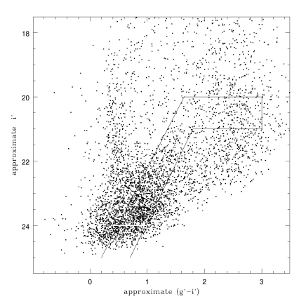
Figure 5: Same as Fig. 4 but for objects rejected because of their high SHARP.

As can be seen in the CMD of Figure 5, the presumably non-stellar objects, rejected because of their high SHARP, show a wide range of colours. One thousand non-stellar objects, with low reddening selected from the SLOAN database, albeit brighter than those seen here, show a huge colour spread. They have a mean $(g^{\prime}-i^{\prime})$ of 1.8 $\pm 1.4$

To investigate the distribution of individual stars, in the plane of the sky, we transform their equatorial coordinates into Cartesian x,y coordinates. We adopt, for the origin: x = 0, y = 0, the coordinates of IC 1613 as given by NED/IPAC, namely: $\alpha$ = 01:04:48.8 and $\delta$ = 02:07:04.0 (J2000.0). Stars fainter than $i^{\prime}$ = 20.0 can be divided into two groups: the blue main sequence stars having $(g^{\prime}-i^{\prime})<-0.3$ and the RGB + AGB stars, in the box drawn on Fig. 4. The spatial distributions of these two populations differ, as can be seen in Figure 6. There are 5000 main sequence stars and 36,500 RGB + AGB stars in this figure. Giants define an elliptical spheroid whose major axis is nearly oriented East - West. The younger main sequence stars are concentrated in an area close to the center but show an off center asymmetry to the center defined by the giants. They also appear to have an elliptical distribution oriented unlike the spheroid. The outer contour and three representative contours of the HI map of IC 1613 obtained by Hoffman et al. (1996) are traced. Lake & Skillman (1989) give 58 $\pm 4^{\circ}$ for the position angle of the major axis of the HI envelope. The RGB stars are nearly all withing the outer isodensity contour. In Fig. 6 (top panel) we also show for comparison the spatial distribution of blue stars. We are awarre that, even though dominated by upper-MS stars, this sample certainly includes older blue supergiants. The spatial distribution of blue stars shows a clear offset relative to the HI and RGB stars.

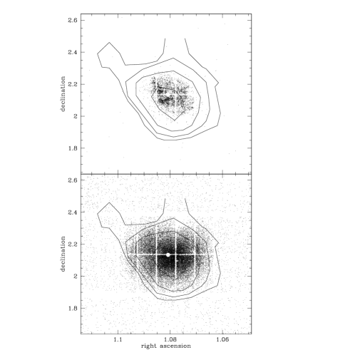
Figure 6: Spatial distributions of the blue main sequence stars (top panel) and RGB + AGB stars (lower panel). Representative HI isodensity contours, from Hoffman et al. (1996) are traced. Each panel corresponds to one square degree of the sky. Big white dots indicate the position of the calculated center.

3.2 Star counts and shape of IC 1613

The gaps between the MegaCam CCDs are far from negligible and need to be filled to better define the stellar surface density distributions. The two wide horizontal empty strips, seen in Fig. 3 above and below the galaxy, ($\approx 80^{\prime\prime}$ wide) are the largest gaps in the mosaic. The narrower vertical gaps (13^′′) are more numerous but not as critical. Lacks of stars here and there are the results of very bright stars contaminating their surrounding. The horizontal gaps are filled by duplicating the observed stellar distribution on a strip of width 40^′′ above and 40^′′ below the gap. Similar fill-up is done for the vertical gaps. Such gap-filling was previously used on MegaCam data by Battinelli et al. (2006). The whole field is then covered by a 50 $\times$ 50 pixel wide grid and stars are counted over a circular 500 pixel sampling area, centered on each intersection of the grid. This is done to smooth out major irregularities (mainly due to bright foreground stars that locally prevent the detection of fainter members of IC 1613.

Figure 7: Solutions for the position angles and ellipticities for elliptical isodensity contours.

The density map is then transformed into a density image that is analyzed with IRAF/STSDAS/ELLIPSE task to fit isodensity ellipses, determine their position angles and ellipticities. The results of this task are summarized in Figure 7 where we show the position angles (PA) and the ellipticities ($\epsilon$) derived for semi-major axes. The PA and $\epsilon$, as expected, vary wildly close to the centre where the stellar surface density is quite patchy and irregular. For distances larger than 4^′ their variations become much less erratics.

For the purpose of the following analysis, we approximate the PA and $\epsilon$ as following: PA = $135^{\circ}$ for r $<4^{\prime}$, decreases linearly to PA = $87^{\circ}$ at r = $7^{\prime}$, then stays constant for r $>7^{\prime}$. Since $\epsilon$ is ill defined for r $<4^{\prime}$, we assume that is its value is equal to its mean value between $4^{\prime}$ and $12^{\prime}$, namely 0.19 $\pm$ 0.02. for r $<12^{\prime}$, it decreases linearly toward zero when reaching r = $22^{\prime}$. The surface density of the elliptical annuli, as defined above, is displayed in Figure 8. The observed density reaches a plateau at r $\sim 23^{\prime}$, we adopt for the foreground + background contributions to the giant counts a density of 0.659 $\pm$ 0.073 “giants” arcmin^-2. This is determined from the mean of the last six points. This number is subtracted from the observed counts, to obtain the corrected surface density.

Figure 8: The observed density profile of the giants. A close up of the tail is shown in the small panel.

The centers of the outer ellipses ($10^{\prime}<r<20^{\prime}$), as determined by the IRAF task, does not match exactly to the origin of the coordinates. Indeed, the mean of the centers is located at a position $48\pm 8^{\prime\prime}$ East and $58\pm 14^{\prime\prime}$ North of the adopted NED/IPAC origin. Therefore, the center of IC 1613 spheroid is then: $\alpha$ = $1^{h}$ 4^m 51.0^s, $\delta$ = $2^{\circ}$ 8^′ 02^′′ (J2000).

3.3 Density profile of the spheroid

Figure 9 displays ln$\rho$, (the corrected surface density) versus the semi-major axis of the ellipses. The error bars are based on the number of stars counted in each annulus. The figure reveals that the density profile deviates from a straight line, excluding, of course, the inner $\sim 5^{\prime}$ where we know that the incompleteness of our counts is more severe. Contrary to the conclusion of Tikhonov & Galazytdinova (2002) who mention that IC 1613 shows an exponential density profile up to 12^′, we observe a pronounced decline to well beyond $20^{\prime}$. This implies that a simple exponential profile does not represent well the whole observed profile. A more complex function, involving more free parameters, must then be sought. King models (King 1962) have been fitted to globular clusters and dSph galaxies (Irwin & Hatzidimitriou 1995; Caldwell et al 1992; McConnachie & Irwin 2006b). For more massive galaxies the Sérsic (1968) law has been considered, see for example Binggeli & Jerjen (1998). We shall compare the observed profile to both King and Sérsic models.

Figure 9: The corrected surface density profile of the spheroid, defined by its giants, is not exponential.

3.3.1 The King profile

The fit of King’s equation to the corrected density profile for $r>5^{\prime}$ is displayed in Figure 10. The adopted fit yields: a corrected central density k = 596 $\pm$ 168 star arcmin^-1, a core radius of $r_{c}$ = 4.54 $\pm 0.93^{\prime}$ and a tidal radius of $r_{t}$ = 24.4 $\pm 0.3^{\prime}$. For the adopted distance of IC 1613, $r_{c}$ = 953 $\pm$ 195 pc and $r_{t}$ = 5.12 $\pm$ 0.06 kpc. This tidal radius is nearly identical to the one deduced by Hodge et al. (1991). The spheroid of IC 1613 is obviously bigger than all known dSphs but its concentration parameter, defined as: c = log${}_{10}({r_{t}\over r_{c}})$, is c = 0.7 a typical value found among dSphs. As expected, our best fitted model gives an overestimate for the central region (dashed line in Fig. 10). Indeed, as discussed in Sect. 2.2, the completeness factor in the central region is significantly lower than elsewhere in the field.

Figure 10: A King model is fitted to the surface density of giants in the spheroid. Dashed line is an extrapolation of the fit. Error bars are omitted to better show the dispersion of the points along the curve.

3.3.2 The Sérsic profile

Sérsic law, more general than an exponential profile, is normally applied to surface brightness profiles. It can also be used for the surface stellar density profile. It is expressed in the following way:

$$\rho=\rho_{o}e^{{-(r/b)}^{n}},$$

It includes a third parameter, $n$, which controls the shape of the profile. Note that many authors use $1/n$ rather than $n$. A fit to our density profile for $r>5^{\prime}$ yields: $\rho_{o}$ = 179.6 $\pm$ 7.9, $b=7.94\pm 0.21^{\prime}$ (1.64 kpc) and $n$ = 1.83 $\pm$ 0.07. The curve corresponding to these parameters is displayed in Figure 11. The value of $n$ is rather large and unusual, indeed, none of the galaxies investigated by Binggeli & Jerjen (1998) have such a large value. The parameter $n$ was found by Caon et al. (1993) to be function of the effective radius ($b$). With a $b=1.64$ kpc, IC 1613 falls off the observed trend because its $n$ is too large. Finally, we note also that the Sérsic fit underestimates the observed central density, this is obviously unrealistic.

Figure 11: A Sérsic law fitted to the observed profile for $r>5^{\prime}$. Dashed line is an extrapolation of the fit.

4 Discussion

At 510 kpc from M31, IC 1613 is currently closer to Andromeda than to the Milky Way. The physical association of IC 1613 with M31 is, however, a matter of debate. Mateo (1998) explains that IC 1613 is an ambiguous case that could be associated with M31 or the MW; while van den Bergh (2000) considers IC 1613 to be a free floating object, isolated in the Local Group. In their recent investigation of the satellite distribution of M31, McConnachie & Irwin (2006a) conclude that the large distance of IC 1613 to M31 makes its membership to the M31 subgroup marginal, see their Fig. 2. Adopting a different point of view, for their mass estimate of M31, Evans & Wilkinson (2000) include IC 1613 among its satellites, on the ground that it is nearer to M31 than to the Milky Way. This question will not be fully solved until the space velocity of IC 1613 relative to M31 is determined.

We believe that the King model gives an appropriate representation of the profile of the spheroid of IC 1613 contrary to the Sérsic profile, traced in Fig. 11. The observed sharp decline of the profile of the spheroid militates in favor of a gravitational association with its nearest big neighbour. However, as often stated, (e.g. McConnachie & Irwin 2006b) a King model is not physically motivated for dSphs or more massive galaxies since their relaxation time is of the order of the Hubble time and their stellar velocity distribution may deviate significantly from Maxwellian. Even if Fornax, the most massive dSph associated with the Milky Way, has a density profile following amazing well a King model (Walcher et al. 2003) any interpretation of the structure of such galaxies based exclusively on the King model fit must be treated with caution.

Notwithstanding this caveat, we could then evaluate, from the determined tidal radius, the distance of nearest approach of IC 1613 to M31. Satellite galaxies are expected to be tidally truncated to the theoretical tidal radius at perigalacticon (Oh & Lin 1992). To do so, we first have to adopt a mass for each galaxy. Contrary to dSphs devoid of gas, IC 1613 has a dynamical mass determined from its HI, we take $8\times 10^{8}$ M_⊙ (Mateo 1998) and $2\times 10^{12}$ M_⊙ for M31 (Evans & Wilkinson 2000). The simple point mass approximation must certainly be skipped for M31. Indeed, its halo is huge having a radius of at least 165 kpc (Kalirai et al. 2006). One other alternative is to adopt a logarithmic potential following Oh et al. (1995) formulation linking the tidal radius (r_t) of the satellite, the eccentricity ($e$) end the semi-major axis (a) of its orbit and the mass ratio ($\alpha$), equal to $4\times 10^{-4}$ in our case. The three variables are linked in the following way:

$$r_{t}=\left[{\alpha(1-e^{2})}\over{[(1-e)^{2}/2e]{\rm ln}[(1+e)/(1-e)]+1}\right]^{1/3}{\rm a}$$

The above equation rules out a circular orbit for IC 1613. When $e\rightarrow 0$ eq. 4 becomes $r_{t}={\rm a}\alpha^{1/3}$ leading to a semi-major axis of 69 kpc, substantially less than the current distance of IC 1613 to M31. However, the application of equation 4 with eccentricities from 0.0 to 0.95 yields a solution for $e=0.78$ and $a=290$ kpc. Such ellipse has a apogalacticon at 517 kpc, close to the actual distance of IC 1613 to M31. The perigalacticon would then be 63 kpc, which is certainly a reasonable minimum distance. However, such large orbit around M31 has a period of $\sim$10 Gyr, that is nearly one Hubble time! Such hypothetical orbit is obviously meaningless because the metric of the Local Group has increased appreciably over the last 10 Gyr.

5 Conclusion

Our wide field survey of IC 1613 confirms Tikhonov & Galazutdinova (2002) finding that no giants of IC 1613 are seen in their HST observations at $27^{\prime}$ and $33^{\prime}$ from its center. The stellar component of IC 1613 is found to extend as far as its observed HI envelope. We note that the young stellar population has a different spatial distribution than the old stars defining the spheroid. The orientation of the HI cloud is appreciably different from the orientation of the stellar spheroid. More pronounced differences between the morphology and orientation of the stellar and gaseous components are seen in NGC 6822, another Local Group dIrr (Battinelli et al. 2006). Nevertheless, IC 1613 dual morphology raises intriguing questions concerning the origin if the HI cloud.

Contrary to the isolated NGC 6822, the spheroid of IC 1613 shows a mark truncation which matches a King density profile. We attribute this feature to the fact that IC 1613 belongs to the M31 system.

- (1) Albert, L., Demers, S., & Kunkel, W. E. 2000, AJ, 119, 2780
- (2) Battinelli, P., Demers, S., & Kunkel, W. E. 2006, A&A, 451, 99
- (3) Binggeli, B. & Jerjen, H. 1998, A&A, 333, 17
- (4) Bland-Hawthorn, J., Vlajić, M., Freeman, K. C., & Draine, B. T. 2005, ApJ, 629, 239
- (5) Caon, N., Capaccioli, M., & D’Onofrio, M. 1993, MNRAS, 265, 1013
- (6) Caldwell, N., Armardroff, T. E., Seitzer, P., & Da Costa, G. S. 1992, AJ, 103, 840
- (7) Demers, S., Battinelli, P., & Kunkel, W. E. 2006, ApJ, 636, L85
- (8) Dolphin, E. D., Saha, A., Skillman, E. D. et al. 2001, ApJ, 550, 554
- (9) Evans, N. W. & Wilkinson, M. I. 2000, MNRAS, 316, 929
- (10) Hodge, P. W., Smith, T. R., Eskridge, P. B. et al. 1991, ApJ, 369, 372
- (11) Hoffman, G. L., Salpeter, E. E., Farhat, B. et al. 1996, ApJS, 105, 269
- (12) Irwin, M. J., & Hatzidimitriou, D. 1995, MNRAS, 277, 1354
- (13) Kalirai, J., Gilbert, K. M., Guhathakurta, P., et al. 2006 ApJ, 648, 389
- (14) King, I. 1962, AJ, 67, 471
- (15) Lake, G. R. & Skillman, E. D. 1989, AJ, 98, 127
- (16) Magnier, E. A. & Cuillandre, J.-C. 2004, PASP, 116, 449
- (17) Mateo, M. 1998, ARAA, 36, 435
- (18) McConnachie, A. W. & Irwin, M. J. 2006a, MNRAS, 365, 992
- (19) McConnachie, A. W. & Irwin, M. J. 2006b, MNRAS, 365, 1263
- (20) Oh, K. S., & Lin, D. 1992, ApJ, 386, 519
- (21) Oh, K. S., Lin, D., N. C., & Aarserth, S. J. 1995, ApJ, 442, 142
- (22) Pietrzyński, G., Gieren, W., Soszyńskui, I. et al. 2006, ApJ, 642, 216
- (23) Sérsic, J.-L. 1968, Atlas de Galaxias Australes, Observatorio Astronomico de Córdoba
- (24) Smith, J. A., Tucker, D. L, Kent, S., et al. 2002, AJ, 123, 2121
- (25) Stetson, P. B. 1987, PASP, 99, 191
- (26) Stetson, P. B. 1994, PASP, 106, 250
- (27) Stetson, P. B. & Harris, W. E. 1988, AJ, 96, 909
- (28) Tikhonov, N. A. & Galazutdinova, O. A. 2002, A&A, 394, 33
- (29) van den Bergh, S. 2000, The Galaxies of the Local Group, Cambridge Astrophysics series: 35
- (30) Vansevičius, V., Arimoto, N., Hasegawa, T., et al. 2004, ApJ, 611, L93
- (31) Walcher, C. J., Fried, J. W., Burkert, A., & Klessen, R. S. 2003, A&A, 406, 807