Effects of QCD phase transition on gravitational radiation
from two-dimensional collapse and bounce of massive stars

Abstract

We perform two-dimensional, magnetohydrodynamical core-collapse simulations of massive stars accompanying the QCD phase transition. We study how the phase transition affects the gravitational waveforms near the epoch of core-bounce. As for initial models, we change the strength of rotation and magnetic fields. Particularly, the degree of differential rotation in the iron core (Fe-core) is changed arametrically. As for the microphysics, we adopt a phenomenological equation of state above the nuclear density, including two parameters to change the hardness before the transition. We assume the first order phase transition, where the conversion of bulk nuclear matter to a chirally symmetric quark-gluon phase is described by the MIT bag model. Based on these computations, we find that the phase transition can make the maximum amplitudes larger up to $\sim$ 10 percents than the ones without the phase transition. On the other hand, the maximum amplitudes become smaller up to $\sim$ 10 percents owing to the phase transition, when the degree of the differential rotation becomes larger. We find that even extremely strong magnetic fields $\sim 10^{17}$ G in the protoneutron star do not affect these results.

I Introduction

It was presented that quark matter may exist in the universe Witten (1984). The existence is now supposed to be inside the core of neutron stars or inferred to be bare quark stars, where several observational signals have been suggested  Drake et al. (2002); Dey et al. (1998); Li et al. (1999); Xu (2005). Much attention has also been paid to explore the relevant astrophysical phenomena in such sites  Bombaci et al. (2004); Drago et al. (2004); Grigorian et al. (2005); Page et al. (2000); Yasutake et al. (2005). Related to the newer observation of PSR J0751+1807, skyrmion stars have been proposed to explain the large mass ($\sim 2.1~{}M_{\odot}$) of a compact object Jaikumar and Ouyed (2006).

It has been presented that the quark matter might appear during supernova explosions Gentile et al. (1993); Takahara and Sato (1986) or the transition of a neutron star to a quark star Berezhiani et al. (2003). Current supernova studies demonstrate that the stellar collapse of stars below $\sim 25M_{\odot}$ in the main sequence stage leads to the formation of neutron stars, while in the case of more massive stars, to the formation of the black hole Heger et al. (2003). In the latter case, quark matters might appear because the central density could exceed the density of the QCD phase transition. It is worth mentioning here that supernova models with the phase transition are important because the vast release of the gravitational energy at the transition could be responsible for some classes of long-duration gamma-ray bursts Yasutake et al. (2005). In this connection, another energy source has been recently proposed as quark nova Ouyed et al. (2002, 2005).

It should be noted that the uncertainty of the equation of state (EOS) is always a big problem in the research of core-collapse supernovae with the phase transition. We might study such microphysical phenomena in the core of the star directly from the detections of the gravitational waves. Currently, the gravitational astronomy is now becoming a reality. In fact, the ground-based laser interferometers such as TAMA300 Ando and the TAMA collaboration (2002, 2005) and the first LIGO Thorne ; Abbott et al. (2005) are beginning to take data at sensitivities where astrophysical events are predicted. For the detectors including GEO600 and VIRGO, core-collapse supernovae especially in our Galaxy, have been supposed to be the most plausible sources of gravitational waves (see reviews, for example, New (2003); Kotake et al. (2006)).

So far, there has been extensive work devoted to studying gravitational radiation in the context of rotational M$\ddot{\textup{o}}$chmeyer et al. (1991); Yamada and Sato (1995); Zwerger and M$\ddot{\textup{u}}$ller (1997); Dimmelmeier et al. (2002); Fryer et al. (2002); Kotake et al. (2003); Shibata and Sekiguchi (2004); Ott et al. (2004) and magnetorotational Kotake et al. (2004); Obergaulinger et al. (2006) core collapse supernovae. On the other hand, there are a very few simulations concerning the effects of the phase transition on the gravitational signals. Lin and his collaborators recently presented a three-dimensional simulation with the use of the polytropic equation of state in baryonic phase and MIT bag model in quark phase. They investigated how the delayed collapse of a rapidly rotating neutron star induced by the phase transition long after its formation, could produce the gravitational waveforms  Lin et al. (2006). They demonstrated that the waveforms can be characterized by the damping timescale of the core and the induced core oscillation frequency. Furthermore, they pointed that the energy release in the form of the gravitational radiation owing to the transition could be less than $\sim 10\%$ of the gravitational binding energy.

In the present paper, we also pay attention to the effects of the phase transition on the gravitational waveforms, not at the epoch considered above, but at the moment of core-bounce during the gravitational collapse of the massive stars. For this purpose, we perform the two-dimensional magnetohydrodynamic (MHD) simulations of the supernova cores accompanying the phase transition. To treat the QCD phase transition, we employ a MIT bag model. We construct the initial models by changing the strength of rotation and magnetic fields, and the degree of differential rotation parametrically. We also vary the hardness of EOS in the baryonic phase in a parametric manner. In this paper, we investigate the relation between the phase transition and the change in the gravitational signals systematically.

This paper is organized as follows. In sec. II we outline the numerical methods, input physics, the initial models, and the numerical methods for the gravitational waveforms. In Sec. III, we present numerical results. Sec. IV is devoted to the conclusion.

II Numerical method and initial models

II.1 Numerical method

The numerical method for MHD computations employed in this paper is based on the ZEUS-2D code Stone and Norman (1992), (see Kotake et al. (2004) for details of the application to the core-collapse simulations). In the following equations, geometric units are used, $G=c=\hbar=1$. The basic MHD equations are written as follows,

$$\cfrac{D\rho}{Dt} +\rho\bm{\nabla}\cdot\bm{v}=0,$$ (1)

$$\rho\cfrac{D\bm{v}}{Dt}=-\bm{\nabla}P -\rho\bm{\nabla}\Phi_{\textmd{eff}}+\cfrac{1}{4\pi}(\bm{\nabla}\times\bm{B})\times\bm{B},$$ (2)

$$\rho\cfrac{D}{Dt}\left(\cfrac{e}{\rho}\right) =-P\bm{\nabla}\cdot\bm{v},$$ (3)

$$\cfrac{\partial\bm{B}}{\partial t} =\bm{\nabla}\times(\bm{v}\times\bm{B}),$$ (4)

$$\Delta\Phi =4\pi\rho.$$ (5)

Here, $\rho,P,\bm{v},e$, $\bm{B}$, $\Phi$, and ${D}/{Dt}$, are the density, pressure, velocity, internal energy density, magnetic field, gravitational potential, and the Lagrangian derivative, respectively. In addition to the previous version Kotake et al. (2004), we newly take into account the general relativistic correction to the Newtonian gravity because it affects the waveform of the gravitational wave at the moment of the phase transition and the subsequent contraction of the core. The effective potential $\Phi_{\textmd{eff}}$ in Eq. (2) includes the correction Marek et al. (2006), which is defined to be

$$\Phi_{\textmd{eff}} = \Phi+\delta\Phi_{\textmd{TOV}},$$

where

$$\delta\Phi_{\textmd{TOV}} = \Phi_{\textmd{TOV}}-\Phi_{\textmd{S}}.$$

Here, $\Phi_{\textmd{TOV}}$ is the gravitational potential which is constructed using the Tolman-Oppenheimer-Volkoff equation. $\Phi_{\textmd{S}}$ is the spherical Newtonian gravitational potential. Albeit simple, this method has been demonstrated to reproduce well the results of the general relativistic calculations  Marek et al. (2006).

II.2 Equation of State

To describe the QCD phase transition in the supernova cores, we follow the method adopted in Ref. Gentile et al. (1993). The transition to a hadronic phase is modeled by adding the MIT bag constant $B$ to the energy density. This phenomenological term lowers the pressure of the quark phase, where a transition to a confined phase occurs.

The EOS in the quark phase is written as :

$$\rho =\cfrac{9}{4}\left(\cfrac{3\pi^{2}}{N_{f}}\right)^{1/3}\left[1+\cfrac{2\alpha_{s}}{3\pi}\right]n_{b}^{4/3}+B,$$ (6)

$$P =\cfrac{3}{4}\left(\cfrac{3\pi^{2}}{N_{f}}\right)^{1/3}\left[1+\cfrac{2\alpha_{s}}{3\pi}\right]n_{b}^{4/3}-B,$$ (7)

$$\mu_{b} =3\left(\cfrac{3\pi^{2}}{N_{f}}\right)^{1/3}\left[1+\cfrac{2\alpha_{s}}{3\pi}\right]n_{b}^{1/3}.$$ (8)

Here, $\rho$ and $\mu_{b}$ are the energy density and the mean baryon chemical potential, respectively. We assume that $\mu_{b}$ is three times that of the quark chemical potential. The number of quark flavors $N_{f}=3$, and $n_{b}$ is the mean baryon number density which is assumed to be the one third of the quark number density. Using (6) and (7), we get :

$$\rho=3P+4B.$$

We assume that the first order phase transition occurs during the collapse beyond some critical density, which has been supported by a recent study about the quark-gluon plasma Glendenning (1992). We set the QCD coupling constant $\alpha_{s}=0$ in most models, which indicates that the coexistence phase between the baryon and quark is the widest in the density region. This choice helps us evaluate the effects of the phase transition maximally Gentile et al. (1993). In the baryon phase, we adopt the phenomenological EOS of BCK Baron et al. (1985) that includes two parameters of the incompressibility $K$ and the adiabatic index $\Gamma$ to express the degree of the hardness of matter above $\rho_{0}$. The EOS of BCK is parametrized as follows,

$$P=\cfrac{Kn_{0}}{9\Gamma}\left[\left(\cfrac{n_{b}}{n_{0}}\right)^{\Gamma}-1\right].$$ (9)

Here the chemical potential in the baryon phase is given as,

$$\mu=\cfrac{\rho+P}{n_{b}},$$ (10)

here $n_{0}$ is the saturation number density ($n_{0}=0.17$ fm^-3), and $\rho_{0}=m_{u}n_{0}$ ($m_{u}$ is the atomic mass unit). Two parameters of $K$ and $\Gamma$ are shown in Table 1. We note that recent measurements give the constraints on the incompressibility : $210\leq K\leq 270$ MeV Itoh et al. (2003); Piekarewicz (2000); Vretenar et al. (2002). Therefore the adopted value of $K=220$ MeV is consistent with this measurement. We furthermore take into account the parameter of $K=375$ MeV, which would correspond to an extreme value. We add the pressures of electrons and photons to the EOS of BCK Gentile et al. (1993). Since we focus on the behaviour of the EOS above $n_{0}$, we use the phenomenological EOS of Ref. Yamada and Sato (1994) below $n_{0}$ in all models.

As for the criterion of the phase transition, we impose the Gibbs condition with respect to the pressure and chemical potential to bridge the baryon and quark phase. We assume that the transition starts at $\rho_{1}=5\times 10^{14}$ g cm^-3 for the baryon phase in most models, whose value lies between those adopted by Gentile et al Gentile et al. (1993). Then, the end point of the transition ($\rho_{2}$) and $B$ are determined analytically from the condition of $P=P_{1}$, $\mu=\mu_{1}$, and $\alpha_{s}=0$ or $0.25$ for the quark phase : $\rho_{2}$ and/or $B(\rho_{1},P_{1},\mu_{1},\alpha_{s})$. Thus, we obtain $\rho_{2}$, $B$, and $\mu_{b}$ for two parameters of $K$ and $\Gamma$ as shown in Table 1. The bag constants used in this paper are consistent with the values used to investigate the structure of hybrid and quark stars Heiselberg and Hjorth-Jensen (2000); Alford et al. (2005).

Table 1: Physical quantities for EOS in hadron/quark phase equilibrium. The values, $\alpha_{s}$, $\rho_{1}$, $\rho_{2}$, $B^{1/4}$, and $\mu_{b}$ are the QCD coupling constant, the critical density of the baryon phase, the density of the corresponding quark phase, the bag constant, and the mean baryon chemical potential, respectively. $K$ and $\Gamma$ are the incompressibility and the adiabatic index, which change the hardness of the baryon phase.

Model	$\alpha_{s}$	$\rho_{1}$ ($10^{14}$g cm-3)	$\rho_{2}$ ($10^{14}$g cm-3)	$B^{1/4}$(MeV)	$\mu_{b}$(MeV)	$K$(MeV)	$\Gamma$
-Mh	0	5	7.34	164.8	967	375	3
-Mm	0	5	7.01	163.8	949	220	3
-Ms	0	5	6.93	163.8	949	220	2.5
-Mma	0.25	5	6.00	157.3	953	220	3
-Mm6	0	6	7.28	163.8	964	220	3

While we get a reasonable value of $\mu_{b}\sim 950$ MeV, $\rho_{1}$ and $\rho_{2}$ are rather low compared to the suggestion from the QCD theory based on the lattice QCD calculations. It is predicted that the transition occurs at $\mu_{b}\geq 1000$ MeV and $\rho_{2}\geq 10^{15}~{}\rm g~{}cm^{-3}$ corresponding to the density of a neutron star Ivanov et al. (2005). We note that the pressure is not constant during the phase transition, since the electron and the photon pressures are included.

II.3 Initial models

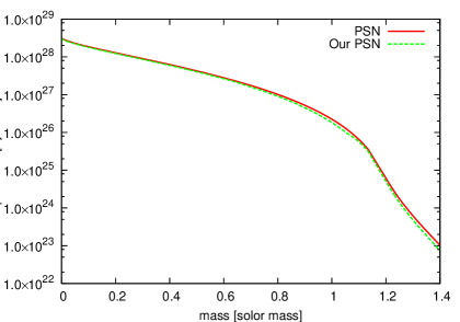
We adopt the presupernova model of 13 $M_{\odot}$ that has the iron core (Fe-core) of 1.2 $M_{\odot}$, in most models. The calculational area extends to 4000 km from the center with the mass of 1.4 $M_{\odot}$ included. FIG. 1 shows the difference of the pressure between the original presupernova model and ours whose EOS is described in Sec. II B. We can see that our EOS is phenomenological but consistent with original one. To examine the mass dependence of presupernova models, we adopt an another presupernova model whose mass is 40 $M_{\odot}$ with the Fe-core of 1.9 $M_{\odot}$. In this model, the calculational area of 4000 km corresponds to 2.4 $M_{\odot}$.

Figure 1: The difference of pressure between the original presupernova model (PSN) and ours (Our PSN), where the region of 1.4 $M_{\odot}$ from the center is shown.

Since the effects of the magnetic field and the angular momentum distribution on the presupernova star are uncertain Heger et al. (2005), we make precollapse models from the nonrotating progenitor model by adding the angular momentum and the magnetic field according to the following prescription. For the initial angular velocity distribution, we adopt the $shell-type$ rotational law Heger et al. (2005):

$$\Omega(r) = \Omega_{0}\times\frac{R_{0}^{2}}{r^{2}+R_{0}^{2}},$$

where $\Omega(r)$ is the angular velocity and $r$ is the radius. Both $\Omega_{0}$ and $R_{0}$ are model constants that prescribe the rotational law. We regard the model with $R_{0}=10^{3}$ km as uniformly rotating, since the radius of Fe core is $\sim 10^{3}$ km. In most initial models, the initial magnetic field is assumed to be constant, $B_{0}$, which is poloidal and parallel to the rotational axis in the computational domain. For the only two models in Table 2, we assume that the initial magnetic field is purely toroidal:

$$B_{\phi}(r) = B_{0}\times\frac{R_{0}^{2}}{r^{2}+R_{0}^{2}},$$

where $B_{\phi}(r)$ is toroidal component of the magnetic fields and $B_{0}$ is a constant. The dominance of the toroidal fields to the poloidal ones is predicted by the recent stellar evolution calculation Heger et al. (2003); Spruit (2002). As is discussed in Sec. III, effects of the magnetic field distribution on the transition are found to be small.

We perform core-collapse simulations of 27 models which are given in Table 2. The characters in the left hand side for each column indicate the initial condition concerning the magnetic fields and rotations: S (spherical), u (weak uniform rotation and weak magnetic field), U (strong uniform rotation and strong magnetic field), R (strong differential rotation), d (strong differential rotation and strong magnetic filed), B (strong differential rotation and strong magnetic field of the $shell-type$ law), D (very strong differential rotation and strong magnetic field). If there is ”40” in the model name, it means that the mass of the presupernava model is 40 $M_{\odot}$. The characters after the hyphen indicate the adopted EOSs. The inclusion of the QCD phase transition is indicated by ’M’: B (BCK without the phase transition), and M (MIT bag model with the phase transition). The right hand side characters mean the hardness for the EOSs in the baryon phase or another choice in the transition parameters. This hardness is expressed by the adiabatic index $\Gamma$ and the incompressibility $K$: h (hard ; $\Gamma=3,K=375$ MeV), m (medium ; $\Gamma=3,K=220$ MeV), and s (soft ; $\Gamma=2.5,K=220$ MeV). Two models u-Mma and d-Mma indicate that $\alpha=0.25$. The model u-Mm6 means that the critical density in baryon phase is $\rho_{1}=6\times 10^{14}$ g cm^-3. We do not calculate the case which corresponds to the model d-Mm, because the rotation of the core is so fast that the maximum density does not reach the critical density.

Table 2: Model parameters. This table is divided into three groups : spherical (S- models), uniform rotation (u, 40u, U- models) and differential rotation groups (d, R, 40d, B, D- models). Note that the models with second capitals of “B” or “M” correspond to those without or with phase transition, respectively.

Model	$\alpha_{s}$	$\rho_{1}$	$K$	$\Gamma$	$R_{0}$	$T/|W|_{\textmd{ini}}$	$E_{\textmd{m}}/|W|_{\textmd{ini}}$	$\Omega_{0}$	$B_{0}$
		($10^{14}$ g cm-3)	(MeV)		(km)	(%)	(%)	($s^{-1}$)	(G)
S-Bm	-	5	220	3	-	-	-	-	-
S-Mm	0	5	220	3	-	-	-	-	-
u-Bh	-	5	375	3	$10^{3}$	0.1	$10^{-3}$	2.3	$6.7\times 10^{10}$
u-Mh	0	5	375	3	$10^{3}$	0.1	$10^{-3}$	2.3	$6.7\times 10^{10}$
u-Bm	-	5	220	3	$10^{3}$	0.1	$10^{-3}$	2.3	$6.7\times 10^{10}$
u-Mma	0.25	5	220	3	$10^{3}$	0.1	$10^{-3}$	2.3	$6.7\times 10^{10}$
u-Mm6	0	6	220	3	$10^{3}$	0.1	$10^{-3}$	2.3	$6.7\times 10^{10}$
u-Mm	0	5	220	3	$10^{3}$	0.1	$10^{-3}$	2.3	$6.7\times 10^{10}$
u-Bs	-	5	220	2.5	$10^{3}$	0.1	$10^{-3}$	2.3	$6.7\times 10^{10}$
u-Ms	0	5	220	2.5	$10^{3}$	0.1	$10^{-3}$	2.3	$6.7\times 10^{10}$
40u-Bm	-	5	220	3	$10^{3}$	0.1	$10^{-3}$	2.1	$9.2\times 10^{10}$
40u-Mm	0	5	220	3	$10^{3}$	0.1	$10^{-3}$	2.1	$9.2\times 10^{10}$
U-Bm	-	5	220	3	$10^{3}$	0.5	$10^{-1}$	5.3	$6.7\times 10^{11}$
U-Mm	0	5	220	3	$10^{3}$	0.5	$10^{-1}$	5.3	$6.7\times 10^{11}$
d-Bm	-	5	220	3	$10^{2}$	0.5	$10^{-1}$	58.8	$6.7\times 10^{11}$
d-Mma	0.25	5	220	3	$10^{2}$	0.5	$10^{-1}$	58.8	$6.7\times 10^{11}$
d-Mm	0	5	220	3	$10^{2}$	0.5	$10^{-1}$	58.8	$6.7\times 10^{11}$
R-Bm	-	5	220	3	$10^{2}$	0.5	-	58.8	-
R-Mm	0	5	220	3	$10^{2}$	0.5	-	58.8	-
40d-Bm	-	5	220	3	$10^{2}$	0.5	$10^{-1}$	79.4	$9.2\times 10^{11}$
40d-Mm	0	5	220	3	$10^{2}$	0.5	$10^{-1}$	79.4	$9.2\times 10^{11}$
B-Bm	-	5	220	3	$10^{2}$	0.5	$10^{-1}$	58.8	$1.3\times 10^{14}$
B-Mm	0	5	220	3	$10^{2}$	0.5	$10^{-1}$	58.8	$1.3\times 10^{14}$
D-Bm	-	5	220	3	50	0.5	$10^{-1}$	183.9	$6.7\times 10^{11}$
D-Mm	0	5	220	3	50	0.5	$10^{-1}$	183.9	$6.7\times 10^{11}$

II.4 Gravitational wave formulae from the rotating magnetized stellar cores

To compute the gravitational waveforms from the rotating and magnetized stellar core, we follow the method of the quadrupole formula derived in Kotake et al. (2004). We describe the gravitational wave amplitude (GWA) $h_{ij}$ that is calculated by

$$h^{\rm TT}_{ij}(R)=\cfrac{2}{R}\cfrac{d^{2}}{dt^{2}}I^{\rm TT}_{ij}(t-R),$$ (11)

where subscripts $i$ and $j$ take over $x$, $y$, and $z$. $t$ is the proper time and $R$ is the distance from the source to an observer, respectively. The superscript TT indicates the transverse traceless part of the metric. $I^{\rm TT}_{ij}$ is the reduced quadrupole moment, defined as

$$I^{\rm TT}_{ij}=\int\rho_{*}(x_{i}x_{j}-\cfrac{1}{3}x^{2}\delta_{ij})d^{3}x,$$

where $\rho_{*}$ is the total energy density including the contributions from the magnetic field,

$$\rho_{*}=\rho+\cfrac{B^{2}}{8\pi},$$ (12)

with $\rho$ being the matter density. The amplitude (11) is then transformed to the spherical coordinate as

$$h^{\rm TT}=h^{\rm TT}_{\theta\theta}=\cfrac{1}{8}\left(\cfrac{15}{\pi}\right)^{1/2}\sin^{2}{\alpha\cfrac{A^{E2}_{20}}{R}},$$ (13)

where $\alpha$ is the angle between the symmetry axis of the source and the direction to the observer and $A^{E2}_{20}$ is the second derivative of the radiative quadrupole $M^{E2}_{20}$,

$$A^{E2}_{20}=\frac{d^{2}}{dt^{2}}M^{E2}_{20}.$$ (14)

$A^{E2}_{20}$ consists of the following two terms:

$$A^{E2}_{20}\equiv A^{E2}_{20,\textmd{quad}}+A^{E2}_{20,\textmd{Mag}}.$$ (15)

Here, $A^{E2}_{20,\textmd{quad}}$ is the contribution from the matter. The magnetic component in Eq. (15) is decomposed into two terms:

$$A^{E2}_{20,\textmd{Mag}}=A^{E2}_{20,\bm{j}\times\bm{B}}+A^{E2}_{20,\rho_{m}},$$ (16)

where $A^{E2}_{20,\bm{j}\times\bm{B}}$ is the contribution from the $\bm{j}\times\bm{B}$ part and $A^{E2}_{20,\rho_{m}}$ is that from the time derivatives of the energy density of the electromagnetic field. In consequence, Eq. (13) is composed of three terms :

$$h^{\textmd{\rm TT}}=h^{\textmd{\rm TT}}_{\rm quad}+h^{\textmd{\rm TT}}_{\bm{j}\times\bf{B}}+h^{\textmd{\rm TT}}_{\rho_{m}},$$ (17)

(see Ref. Kotake et al. (2004) for details). In the following, we assume that the distance from the observer ($R$) is 10 kpc in the direction of the equator ($\alpha=\pi/2$).

III Numerical results

We summarize the physical quantities obtained from the numerical simulations in Table 3. As a guide to see the effects of the phase transition on the maximum amplitudes, we prepare the following quantity,

$$\Delta|h^{\textmd{\rm TT}}|_{\textmd{max}}=\cfrac{|h^{\textmd{\rm TT}}_{M}|_{\textmd{max}}-|h^{\textmd{\rm TT}}_{B}|_{\textmd{max}}}{|h^{\textmd{\rm TT}}_{B}|_{\textmd{max}}},$$ (18)

where $|h^{\textmd{\rm TT}}_{M}|_{\textmd{max}}$ and $|h^{\textmd{\rm TT}}_{B}|_{\textmd{max}}$ are the absolute value of gravitational wave amplitudes (GWAs) with and without the phase transition, respectively.

From the table, we can see that the phase transition makes the maximum GWAs larger by a few up to $\sim$ 10 percents for the uniformly rotating models. On the other hand, the phase transition lowers the maximum GWAs for the differentially rotating models. If the rotational strength $T/|W|$ becomes very large, the effects of phase transition on gravitational waves become small. We explain these features in the following subsections, where the changes in GWA from models to models are examined. Furthermore, we perform the Fourier transformations for all models to show more comprehensive and systematic analysis of the gravitational waveforms.

Table 3: Physical quantities for the models with and without the phase transition. $t_{b},\,t_{\textmd{fin}}$ and $\rho_{\textmd{max}}$ are the bounce time, the final time of the calculation, and the maximum density. $T/|W|_{\textmd{fin}}$ and $E_{\textmd{m}}/|W|_{\textmd{fin}}$ are the final values of $T/|W|$ and $E_{\textmd{m}}/|W|$, respectively. $|h^{\textmd{\rm TT}}|_{\textmd{max}}$ is the maximum GWA, and $\Delta|h^{\textmd{\rm TT}}|_{\textmd{max}}$ is defined by Eq.(18). Note that models with second capitals of “B”, “M” corresponds to without and with phase transition, respectively. $f_{1st}$ is the first peak frequency in the Fourier transformation of GWA.

Model	$t_{b}$	$t_{\textmd{fin}}$	$\rho_{\textmd{max}}$	$T/|W|_{\textmd{fin}}$	$E_{\textmd{m}}/|W|_{\textmd{fin}}$	$|h^{\textmd{\rm TT}}|_{\textmd{max}}$	$\Delta|h^{\textmd{\rm TT}}|_{\textmd{max}}$	$f_{1st.}$
	(ms)	(ms)	(1014g/cm3)	(%)	(%)	($10^{-20}$)	(%)	(Hz)
S-Bm	75.5	126	6.95	-	-	-	-	-
S-Mm	75.5	146	8.84	-	-	-	-	-
u-Bh	76.3	82.6	5.37	1.24	2.12 $\times 10^{-3}$	0.28	-	727
u-Mh	76.3	82.7	6.72	1.24	2.05 $\times 10^{-3}$	0.29	+3.6	748
u-Bm	76.2	82.7	6.90	1.29	2.07 $\times 10^{-3}$	0.31	-	652
u-Mma	76.3	87.2	7.19	1.31	2.24 $\times 10^{-3}$	0.32	+3.2	652
u-Mm6	76.2	83.4	8.05	1.27	2.24 $\times 10^{-3}$	0.33	+6.4	838
u-Mm	76.3	87.0	8.60	1.33	4.27 $\times 10^{-3}$	0.34	+9.6	875
u-Bs	76.3	83.3	8.12	1.29	2.25 $\times 10^{-3}$	0.34	-	587
u-Ms	76.2	86.6	8.79	1.36	3.28 $\times 10^{-3}$	0.38	+11.8	931
40u-Bm	70.6	76.1	7.02	1.29	4.15 $\times 10^{-2}$	0.26	-	635(889)
40u-Mm	70.7	79.4	8.64	1.39	5.42 $\times 10^{-2}$	0.28	+7.6	762
U-Bm	79.3	86.0	6.35	5.05	5.32 $\times 10^{-2}$	1.25	-	859
U-Mm	79.4	93.2	8.03	4.97	8.25 $\times 10^{-2}$	1.27	+1.6	872
d-Bm	83.8	90.9	5.64	9.41	1.16 $\times 10^{-1}$	3.03	-	792
d-Mma	83.8	91.0	6.27	9.52	1.15 $\times 10^{-1}$	2.79	$-$7.9	743
d-Mm	83.8	91.0	7.31	9.40	1.14 $\times 10^{-1}$	2.72	$-$10.2	659
R-Bm	83.8	90.9	5.67	9.53	-	3.03	-	791
R-Mm	83.8	91.0	7.40	9.51	-	2.71	$-$10.6	658
40d-Bm	84.1	89.9	5.81	12.8	1.33 $\times 10^{-1}$	2.98	-	562
40d-Mm	84.3	90.1	7.50	12.3	1.40 $\times 10^{-1}$	2.72	$-$8.7	494
B-Bm	84.1	91.0	5.57	9.51	1.61 $\times 10^{-1}$	2.96	-	668
B-Mm	84.2	91.2	7.29	9.49	1.62 $\times 10^{-1}$	2.69	$-$9.1	668
D-Bm	83.9	90.9	5.21	8.33	1.59 $\times 10^{-1}$	3.02	-	814
D-Mm	83.9	91.1	7.32	8.36	1.47 $\times 10^{-1}$	2.74	$-$9.3	780

III.1 Effects of the phase transition and rotation

We will first show the effects of the phase transition on GWA for the uniformly rotating models. We find that GWAs are larger from a few percents to about ten percents by considering the phase transition for all uniformly rotating models as seen in Table 3 and FIGs. 2-6.

Figure 2: GWAs as a function of time in u-Mh and u-Bh models (left) and the corresponding Fourier transformations (right).

Figure 3: Same as FIG. 2 but for u-Mm and u-Bm.

Figure 4: Same as FIG. 2 but for u-Ms and u-Bs.

Figure 5: Maximum density and radiative quadrupole moment of the model u-Mh and u-Bh.

Figure 6: Same as FIG. 6 but for u-Mm and u-Bm.

Figure 7: Same as FIG. 6 but for u-Ms and u-Bs.

Figure 8: Same as FIG. 2 but for models of 40u-Mm and 40u-Bm.

Figure 9: Same as FIG. 2 but for the models of u-Mm and u-Mma.

Figure 10: Same as FIG. 2 but for the models of R-Mm and R-Bm.

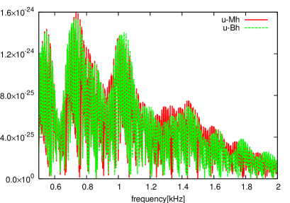
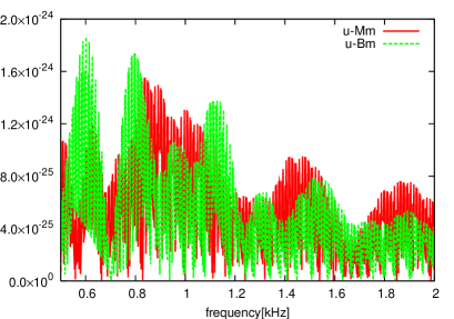
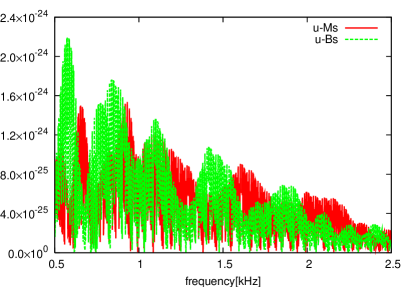
As the initial rotational strength $T/|W|_{\textmd{ini}}$ increases, the maximum GWA, $|h^{\rm TT}|_{\textmd{max}}$ becomes large. However the effect of the phase transition on the maximum GWA decreases as seen from $\Delta|h^{\textmd{TT}}|_{\textmd{max}}$. In the right panels of FIGs. 2-6, we can see that the frequency region with the phase transition shifts to the higher one as a whole, because the increased density during the collapse tends to the higher frequency  Lin et al. (2006). As for the effects of the equation of state, we find that the larger gravitational wave is radiated for the soft EOS, regardless of the phase transition. Comparing the models of hard, medium and soft EOS in Table 3, this tendency is recognized to be independent on whether the softness originates from $\Gamma$ or $K$.

To understand these results, we give an order-of-magnitude estimation of the quadrupole formula Yamada and Sato (1994); Kotake et al. (2004). The gravitational amplitude is proportional to the second time derivative of the radiative quadrupole (see Eqs. (13) and (14)). The second time derivative in Eq. (14) could be replaced by the reciprocal of the square of the time, if the time scale is very short. The typical dynamical time scale of the collapsing core is $t_{\rm{dyn}}\sim 1/\sqrt{G\rho}$. As the result, the amplitude is roughly proportional to the core density $\rho_{c}$ multiplied by the radiative quadrupole moment:

$$h^{\rm TT}\propto\rho_{c}M^{E2}_{20}.$$ (19)

The leftsides of Figs. 6-7 show the time dependence of the maximum density. The maximum density of the model with the phase transition (for example the model of u-Mm) is always larger than that without the transition (for example the model of u-Bm). In the figures of $\rho_{max}$ and their corresponding GWA figures, there are high frequency spikes. However, these are numerically ones, because quark matter areas ($\sim$ 10 km) are much smaller than overall calculational areas (about Fe-core size). More fine tuned calculations with many meshes will delete such spikes. The absolute values of $M^{E2}_{20}$ are almost the same around the peak, if the initial rotational strengths are the same (see the right panels of Figures 6-7). Since the transition causes the increase in the density being similar to the effect of soft EOS, we get larger amplitudes. $|h^{\rm TT}|_{\textmd{max}}$ in u-Ms increases by 10% compared to u-Bs as seen in Table 3. On the contrary, we find that the effect of the phase transition becomes small if the rotational strength becomes as large as $T/|W|_{\textmd{fin}}\simeq 5\%$, which leads to the suppression of the contraction due to the strong centrifugal forces (compare $\rho_{\textmd{max}}$ of u-Mm with that of U-Mm in Table 3).

For the Fourier transformations, the ranges of frequencies are distributed in 500-2000 Hz for all models. Clear peaks are not found compared to the case in Ref. Lin et al. (2006). While we adopt realistic presupernova models as initial models, they use polytropic models of equilibrium neutron stars. If QCD phase transition is considered, both the soft EOS model (FIG. 6) and slowly rotating model (FIG. 6) result in the shift to the high frequency sides in proportion to the increased density during the collapse (see $f_{1st.}$ of the models with/without the transition in Table 3).

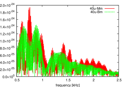
To check the effects on GWA due to the difference of presupernova models, we calculate the collapse of 40 $M_{\odot}$ models. The result is given in Table III (compare model 40u-Mm with u-Mm, or 40d-Mm with d-Mm). We see the difference of the maximum density at the bounce, which is ascribed to the size of the Fe-core. The slight differences of the maximum amplitudes are found between the models with/without the phase transition. The difference of the presupernova models dose not make a qualitative difference in both uniformly rotating and differentially rotating models. In the Fourier transformation, the overall frequencies for 40u-Mm shift to the higher region compared to the case of 40u-Bm as seen in FIG. 10 except for around $f_{1st}$, where the first peak is not clear.

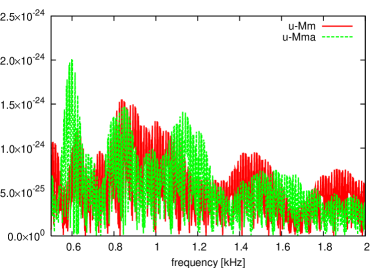
We change a value of coupling constant $\alpha_{s}$. As the width of the density during the phase transition (coexistence area) becomes narrower for $\alpha_{s}\neq 0$, the difference of the amplitude by the presence of the phase transition should become small. In Table 3, the value $|h^{TT}|_{max}$ of u-Mma is between u-Mm and u-Bm. In the Fourier transformation, the change in $f_{1st}$ is small, but the frequencies shift overall between those of u-Mm and u-Bm (see Table 3 and FIG. 10). In differentially rotating model, GWA and the frequencies of d-Mma lie between those of d-Mm and d-Bm, too.

The difference of critical density ($\rho_{1}$) for the gravitational wave is shown in Table 3. The higher critical density (u-Mm6) results in the narrower width of the density region during the transition. As a consequence, $|h^{TT}|_{max}$ and $f_{1st}$ of u-Mm6 are between the corresponding values of u-Mm and u-Bm.

For the strong differential rotation, it is shown in Table 3 and FIG. 10 that the maximum amplitudes become smaller for the models with the phase transition (see $\Delta|h^{\textmd{TT}}|_{\textmd{max}}$ of the three models, from the bottom in table 3). To explain such aspects, we refer to the early research Obergaulinger et al. (2006). Their results show that very fast rotation with soft EOS models tend to suppress the centrifugal force element of GWA. Here very fast rotation is not limited in differential rotation, but includes very fast uniform rotation whose $T/|W|$ is one digit larger than our uniformly rotating models. Since our initial models are spherical models, we do not adopt such a large $T/|W|$ for consistency with our initial models. Consequently, the strong differentially rotating models with the transition in our calculations are the same as very fast rotation with soft EOS, which lowers 1st peak of GWA for our differentially rotating models shown in Table III. Corresponding to these, their frequencies with the transition shift to low (see their Fourier transformation, FIG. 10 and $f_{1st.}$s of Table 3). The above estimate (19) is useful for the interpretation of the results. However it is found to be not applicable for strong differential rotation. This is because the differential rotation acts against a matter infall to the center by the phase transition due to the stronger centrifugal forces, but simultaneously leads to the stronger accretion to the center due to the smaller angular momentum in the rather outer regions. Due to this very subtle competition, we can only know from the numerical results that the differential rotation makes the amplitudes lower up to $\sim$ 10 percents at the moment of the phase transition as far as the parameters in the present calculations.

III.2 Effects of the phase transition and magnetic fields

We focus on the models with the strongest magnetic fields (”B$-$” models in Table 2) to clarify the effects of the magnetic field on the gravitational wave. First, we compare each component $h^{\rm TT}_{\textmd{quad}}$, $h^{\rm TT}_{\bm{j}\times\bm{B}}$ and $h^{\rm TT}_{\rho_{m}}$ of $h^{\rm TT}$ in Eq.(17). Figure 11 shows the waveforms originated from the mass quadrupole moment, $\bm{j\times B}$ part, and the time derivative of the magnetic energy density $\rho_{m}$. The most definitive component to GWA is the one originated from the mass quadrupole moment $h^{\textmd{\rm TT}}_{\rm quad}$.

Figure 11: Waveforms of the strong magnetized models, B-Mm and B-Bm. The top figure is one originated from the mass quadrupole moment, the next figure is from $\bm{j}\times\bm{B}$ part and the bottom is from the time derivatives of the magnetic energy density $\rho_{m}$. Note the scale differences of the vertical axis.

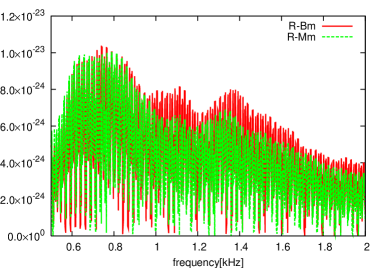
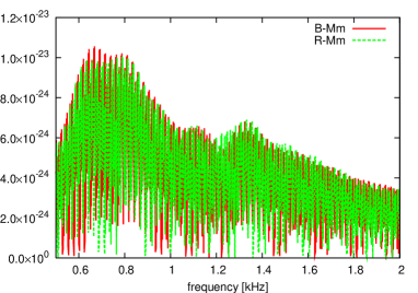
To see the influence of the magnetic field on the gravitational wave frequencies, we compare the zero magnetic field models (R-Bm, R-Mm) with strong magnetic field ones (B-Bm, B-Mm). It is understood from FIG 10-12 that the influence of the magnetic field with the transition on the gravitational wave can be neglected. The corresponding maximum GWAs have almost the same values as shown in Table 3.

Figure 12: Fourier transformation of waveforms for the strongly magnetized model B-Mm and unmagnetized model R-Mm, corresponding to GWAs of FIG. 10 and FIG. 11 .

The components of GWA for B-Bm and B-Mm are summarized in Table 4. It should be noted that sign of each component at the bounce is different in the strong magnetic field models. As the result of cancellation between $h^{\textmd{\rm TT}}_{\textmd{quad}}$ and $h^{\textmd{\rm TT}}_{j\times B}$, the ratio of $|h^{\textmd{\rm TT}}_{j\times B}/h^{\textmd{\rm TT}}_{\textmd{quad}}|$ becomes less than 8 % regardless of the phase transition, which can be roughly estimated by the ratio of the magnetic to the matter energy density at bounce, namely,

$$\cfrac{B^{2}_{c}}{8\pi}\cdot\rho_{c}^{-1}\sim O(1)~{}\%(\cfrac{B_{c}}{10^{17}\textmd{~{}G}})^{2}(\cfrac{\rho_{c}}{10^{14}\textmd{~{}g~{}cm}^{-3}})^{-1}.$$ (20)

Kotake et al. (2004) Kotake et al. (2004) have found the same effect though they did not include the phase transition. In fact, we can see from Table 3 that GWAs of the model B-Bm (B-Mm) is smaller compared to other models R-Bm (R-Mm) due to this contribution from the magnetic fields.

At the moment of the phase transition, the magnetic fields in the central regions become larger due to the compression, because the magnetic fields are frozen-in to the matter. As a result, the contribution to the amplitudes from the magnetic fields become larger for the model with the transition, but the change is found to be as small as 1% (compare $|h^{\textmd{\rm TT}}_{j\times B}/h^{\textmd{\rm TT}}_{\textmd{quad}}|$ in table 4.)

Table 4: Three components in Eq. (17). Note that the listed values correspond to the time when the values of $|h^{\textmd{\rm TT}}_{j\times B}/h^{\textmd{\rm TT}}_{\textmd{quad}}|_{max}$ is maximum. It means that the time is not same with the time of $|h^{\textmd{\rm TT}}|_{\textmd{max}}$ in table 3. All amplitudes are given in units of $10^{-20}$.

Model	$h^{\textmd{\rm TT}}_{\textmd{quad}}$	$h^{\textmd{\rm TT}}_{j\times B}$	$h^{\textmd{\rm TT}}_{\rho_{m}}$	$|h^{\textmd{\rm TT}}_{j\times B}/h^{\textmd{\rm TT}}_{\textmd{quad}}|_{max}$(%)
B-Bm	$-$3.06	1.99$\times 10^{-1}$	$-$3.24 $\times 10^{-9}$	6.5
B-Mm	$-$2.80	2.16$\times 10^{-1}$	$-$3.61$\times 10^{-9}$	7.7

IV Conclusion

We have performed two-dimensional axisymmetric, magnetohydrodynamical simulations for supernova cores accompanying the QCD phase transition. To elucidate the implications of a phase transition against a supernova, we investigated how the phase transition affects the gravitational waveforms near the epoch of core-bounce. As for the initial models, we changed parametrically the strength of the rotation and the magnetic fields. As for the microphysics, we adopted a phenomenological equation of state above the nuclear matter density, including two parameters to change the hardness of the matter before the transition. To treat the QCD phase transition, we employed a MIT bag model. Based on these computations, we showed that the phase transition can make the maximum amplitudes larger up to $\sim$ 10 percents than the ones without the phase transition. On the other hand, we found that the phase transition makes the maximum amplitudes smaller up to $\sim$ 10 percents, when the iron core rotates strongly differentially. It was confirmed that the strong magnetic fields themselves decrease the maximum amplitudes by less than 8% regardless of the transition. Even the extremely strong magnetic fields $\sim 10^{17}$ G in the protoneutron star do not affect the above features.

Finally, we give some discussions and speculations based on the obtained results. We assume rather low density for the onset of the phase transition in comparison with a recently predicted EOS by the lattice QCD computations Ivanov et al. (2005). Thus the results here could be some extreme cases predicted by the phenomenological MIT bag model, and the change in the amplitudes due to the transition could be interpreted as an upper bound.

Although the other initial presupernova models may change our analysis to some extent, the qualitative results obtained here will not be different so much. This is because the structure of the iron core is similar, while the initial mass of the helium core increases with the progenitor masses Hashimoto (1995). For the presupernova model of $40M_{\odot}$ that has the iron core of 1.9$M_{\odot}$, we have found that GWA at the bounce is only about 3 percents larger than that of 13$M_{\odot}$. Since we concentrate on the forms of the gravitational wave just after the bounce, the difference in the helium core mass should not be important at all.

If we could calculate the hydrodynamical evolution long after the core bounce especially in some failed core-collapse supernova models, we would observe the phase-transition of the protoneutron stars. We also think interesting to investigate the possible effects of color-superconductivity recently proposed Ker$\ddot{\textup{a}}$nen et al. (2005). As a next step, we are now going to investigate how the gravitational waves will be originated from such events in the context of magnetorotational core-collapse.