Molecular oxygen in the $\rho$ Ophiuchi cloud

Abstract

Context. Molecular oxygen, O₂, has been expected historically to be an abundant component of the chemical species in molecular clouds and, as such, an important coolant of the dense interstellar medium. However, a number of attempts from both ground and from space have failed to detect O₂ emission.

Aims. The work described here uses heterodyne spectroscopy from space to search for molecular oxygen in the interstellar medium.

Methods. The Odin satellite carries a 1.1 m sub-millimeter dish and a dedicated 119 GHz receiver for the ground state line of O₂. Starting in 2002, the star forming molecular cloud core $\rho\,{\rm Oph\,A}$ was observed with Odin for 34 days during several observing runs.

Results. We detect a spectral line at $v_{\rm LSR}$ $=+3.5$ km s^-1 with $\Delta v_{\rm FWHM}=1.5$ km s^-1, parameters which are also common to other species associated with $\rho\,{\rm Oph\,A}$. This feature is identified as the O₂ ($N_{J}=1_{1}-1_{0}$) transition at 118 750.343 MHz.

Conclusions. The abundance of molecular oxygen, relative to H₂ , is $5\times 10^{-8}$ averaged over the Odin beam. This abundance is consistently lower than previously reported upper limits.

1 Introduction

O₂ is an elusive molecule that has been the target of two recent searches using the Submillimeter Wave Astronomy Satellite (SWAS, Goldsmith et al., 2000) and Odin (Pagani et al., 2003). Previous attempts included the search for O₂ with the balloon experiment Pirog 8 (Olofsson et al., 1998) and the search for the rarer isotopomer ¹⁶O¹⁸O with the Radio telescope millimetrique POM-2 (Maréchal et al., 1997) and the Caltech Submillimeter Observatory (CSO) (van Dishoeck, Keene & Phillips, private communication) from the ground. These unsuccessful searches implied very low O₂ abundances, a highly intriguing result which led Bergin et al. (2000) to make several suggestions aimed at understanding the low O₂ abundance. A number of subsequent chemical models focused on innovative solutions to understand the interstellar oxygen chemistry (e.g., Charnley et al., 2001; Roberts & Herbst, 2002; Spaans & van Dishoeck, 2001; Viti et al., 2001; Willacy et al., 2002).

As these models had to rely on upper limits and, as such, were not very well constrained, it seemed likely that an actual measurement of the O₂ concentration would increase our understanding of molecular cloud chemistry. For this reason, Odin has continued the time-consuming task of observing O₂. Here, we report on our renewed efforts to detect O₂ toward $\rho\,{\rm Oph\,A}$. First results have been announced previously by Larsson et al. (2005) and by Liseau et al. (2005); however, in this paper, we also account for additional data which were collected in 2006.

2 Odin observations

The O₂ observations were done in parallel while Odin was mapping the $\rho\,{\rm Oph\,A\,cloud}$ in molecular lines in the submillimeter bands (submm). These observations were made in August 2002, September 2002, and February 2003 during 20 days of satellite time (300 orbits), with an additional 200 orbits in February 2006. Due to Earth occultation, only two thirds of the 97 min orbit are actually available for astronomy. The total on-source integration time was 77 hours in 2002, 52 hr in 2003, and finally 68 hr in 2006.

At the frequency of the ${\rm O}_{2}\,(N_{J}=1_{1}-1_{0})$ line (118 750.343 MHz), the beam of the 1.1 m telescope is 10^′ (Fig. 1). This large beam implies that the Odin pointing uncertainty ($\leq 15$^′′) is entirely negligible for the O₂ observations. In the submm mapping mode, the O₂ beam moved by less than $1/5$ of its width with respect to the center position at RA = 16^h26^m24$\stackrel{{\scriptstyle\rm s}}{{{}_{\bf\cdot}}}$6 and Dec = $-24$^∘23^′54^′′ (J2000). The observed off-position, supposedly free of molecular emission, was 900^′′ north of these coordinates.

The observing mode was Dicke-switching with the 4$\stackrel{{\scriptstyle\circ}}{{{}_{\bf\cdot}}}$7 sky-beam pointing off by $42$^∘ (Frisk et al., 2003; Olberg et al., 2003). The front- and back-ends were, respectively, the 119 GHz receiver and a digital autocorrelator (AC) with resolution of 292 kHz, channel separation 125 kHz (0.32 km s^-1 per channel) and bandwidth 100 MHz (250 km s^-1). The 119 GHz mixer is fixed-tuned to suppress the undesired sideband (Frisk et al., 2003). Individual spectral scans were 5 s integration each. The system noise temperature, $T_{\rm sys}$, was 650 K (single sideband) in 2002 and 750 K in 2003. In 2006, the $T_{\rm sys}$ had increased significantly to 1 100 - 1 300 K, so these data did not provide any improvement to the signal-to-noise ratio.

Figure 1: The 10^′ Odin beam at 119 GHz, the frequency of ${\rm O}_{2}\,(N_{J}=1_{1}-1_{0})$, is shown as the large circle superposed onto the 450 $\mu$m map by Hargreaves (2004) (see also Wilson et al., 1999). At the distance of 145 pc (de Zeeuw et al., 1999), the beam size corresponds to 0.4 pc. A few discrete sources are labelled. The observations were centered on RA = 16^h26^m24$\stackrel{{\scriptstyle\rm s}}{{{}_{\bf\cdot}}}$6, Dec = $-24$^∘23^′54^′′ (J2000).

In contrast to the Odin O₂ search by Pagani et al. (2003), the receiver was no longer phase-locked during the observations of $\rho\,{\rm Oph\,A}$ reported here. However, Odin ‘sees’ the Earth’s atmosphere for a third of an Odin revolution. Accurate frequency standards are thus provided by the telluric oxygen lines.

Figure 2: The Hanning-smoothed O₂ line spectrum is shown in the bottom panel and compared to Odin H₂O ($1_{1,\,0}-1_{0,\,1}$) line data (Larsson et al., 2007), to C¹⁸O ($3-2$) and CO ($3-2$) from the JCMT-archive, and the C $158\alpha$ recombination line from Pankonin & Walmsley (1978). The H₂O spectrum represents the average of the part of the $\rho\,{\rm Oph\,A\,cloud}$ mapped with Odin (slightly larger than 5^′ $\times$ 4^′). The C¹⁸O spectrum (15^′′ beam) refers to a pointed observation toward the Odin center coordinates, while the CO spectrum is that of the 3$\stackrel{{\scriptstyle\prime}}{{{}_{\bf\cdot}}}$5 $\times$ 10^′ (at PA=45^∘) CO ($3-2$) map convolved with the 10^′ Odin beam. The displayed spectrum of the C $158\alpha$ recombination line refers to the average of 4 map positions covering about 10^′ $\times$ 10^′. Vertical dotted lines are shown at $v_{\rm LSR}=+3.0$ km s^-1 and $+4.5$ km s^-1, respectively.

3 The data reduction

The data reduction method is described in considerably greater detail in Appendix A. For the purpose of the following discussion, it suffices to mention that, because of dramatic frequency variations and receiver instabilities, roughly 50% of the O₂ search data were of too low quality and therefore not included in the final merged spectrum (see Fig. 2). The calibrated spectral data are given in the $T_{\rm A}$ scale. The in-flight main beam efficiency of Odin in the mm-regime, i.e. at 119 GHz, is unknown, but is expected not to be much worse than the submm main beam efficiency, which has been determined as $\eta_{\rm mb}=0.9$ (Frisk et al., 2003; Hjalmarson et al., 2003).

Figure 3: The normalized antenna temperature noise distribution. To render the data points statistically independent they have been reduced into bins containing 5 channels. As shown in the figure, the statistics of the noise (histograms) are all consistent with Gaussian distributions (smooth lines). The letters A and B designate two independent data sets and the entire data set is displayed at the bottom of the figure. The respective $4\sigma$ and $5\sigma$ locations of the O₂ line are shown by the filled-in symbol of the observations.

Table 1: Results for O₂ observations of $\rho\,{\rm Oph\,A}$

Parameter†	Value‡
Gaussian fit
$v_{\rm LSR}$, 0 (km s-1)	$3.5\pm 0.3\>(\pm 0.5)^{\#}$
$T_{0}$ (mK)	$17.4\pm 0.1\>(\pm 0.5)^{\#}$
$\Delta v_{\rm FWHM}$ (km s-1)	$1.5\pm 0.4\>(\pm 0.5)^{\#}$
$T_{\rm rms}$ (mK)	$3.1$
S/N	$5.6$
Data 5 channels rebinned
$T_{0}$ (mK)	$16.0$
$T_{\rm rms}$ (mK)	$2.7$
S/N	$5.9$
$\int\!T{\rm d}v$ (mK km s-1)	$24\pm 4$
$N$(O2) (1015 cm-2)	1§

Notes to the Table:
^† Temperatures are in the antenna temperature scale, $T_{\rm A}$. $T_{0}$ are line center and peak temperatures, respectively. $T_{\rm rms}$ are the fluctuations about the zero-$T$ level over the useful bandwidth, $\Delta v\sim 180$ km s^-1.
^‡ Gaussian values refer to the AC resolution of 0.3 km s^-1 per channel.
^# Including error estimate from the frequency restoration uncertainty.
^§ For optically thin emission in thermodynamic equilibrium at 30 K.

4 Results

A part of the O₂ spectrum is shown in Fig. 2, where it is also compared to other spectral lines. At the top, the observation of a recombination line of carbon is shown (Pankonin & Walmsley, 1978). Below that, the spectrum of the CO ($3-2$) line from the JCMT archive (James Clerk Maxwell Telescope) shows the spectrally resolved CO emission averaged over the mapped $\rho\,{\rm Oph\,A\,cloud}$. The observation in C¹⁸O ($3-2$) is toward the center position of the Odin map and the spectrum of the mapped H₂O ($1_{1,\,0}-1_{0,\,1}$) line (Larsson et al., 2007) is displayed below the CO data. It is noteworthy that the O₂ emission feature shares the velocity of the self-absorption feature seen in the optically thick CO and H₂O lines.

The Odin data over the full spectral range of about 180 km s^-1 are displayed in Fig. 11. The reduction from the initially available 250 km s^-1 to the finally usable 180 km s^-1 bandwidth is due to the fact that some of the channels will be lost when reducing the data (non-matching alignment; see the figure in Appendix A).

In addition to the line at the O₂ frequency, a feature at three times the rms level can be seen at the relative Doppler velocity of $+21.0$ km s^-1 (Fig. 10). The corresponding frequency is 118 742.0 MHz, which coincides with the rest frequency of the $(3_{2,\,2}-2_{1,\,1})$ transition of ethylene oxide of 118 741.9 MHz (Pan et al., 1998). The apparent difference of 100 kHz is within the channel separation of 125 kHz. Ethylene oxide, c-C₂H₄O, has been observed in a number of warm and dense clouds by Ikeda et al. (2001).

5 Discussion

5.1 The validity of the O₂ line detection

The O₂ feature is burried deeply in the Odin data and its extraction requires great care to be taken. This could initially be seen as a weakness and therefore calls for a rigorous assessment of the validity of the claimed detection. In the following, we will present arguments which make the possibility that the observed signal is of spurious origin highly unlikely.

5.1.1 Statistical character of the noise

Neighbouring spectrometer channels are not independent of each other and the original data have therefore been re-binned to the measured width of the line (5 channels, see the Appendix A). The resulting distributions of the noise are shown in Fig. 3, where the fit to a normalized normal distribution of the combined data set yields a $\sigma$ of 3.0 mK. As is evident from Fig. 3, the statistical significance of the detection of the O₂ line is at the $5.4\sigma$ level.

The probability that the observed line is a noise feature is thus less than $5\times 10^{-6}$. Furthermore, and very significantly, this line is found at the expected Doppler velocity of the $\rho\,{\rm Oph\,A\,cloud}$ and since the number of independent velocity-channels is of the order of one hundred, this probability is further reduced to below $5\times 10^{-8}$. This would apply to a single data set of observations. This conclusion can be further strengthened by dividing the data into two independent data set (see Appendix A) and performing the same analysis on both sets.

As is evident from Fig. 11, the line is clearly detected at the correct velocity in both data sets A and B, at the level of $4.0\sigma$ and $4.2\sigma$, respectively (see Fig. 3). The corresponding probability for being pure noise is less than $4\times 10^{-5}$ and $2\times 10^{-5}$, respectively. The probability that a pure noise feature will apeare twice at the same channel will therefore be less than $8\times 10^{-10}$.

5.1.2 Systematic effects

So far, we have considered the nature of the noise only in a statistical sense, but there might of course also be sources of systematic errors. Fortunately however, any narrow ($<10$ km s^-1) features would be smeared out, when the frequency correction for the drift, both from the unlocked receiver and the satellite motion, is made.

Of concern could also be that the integration time spent on the hot load is much less than that spent on the source. Therefore, as is explained in the Appendix A, we approximated $T_{\rm sys}$ with a single value to prevent possible spectral artefacts from the hot load measurement from entering the observational data.

Another concern could be that the line in the final spectrum is located near the edge of the spectrum. However, more than one third of the finally used data stems from the 2003 observing campaign. During that period, however, the line was situated in the middle of the spectrometer band (see the lower right panel in Fig. 6). Therefore, irrespectively of its location in the spectrometer band, the line is consistently detected at the common (correct LSR-) velocity.

Another problem could be due to leakage from the other sideband. However, to the best of our knowledge there are no spectral lines in the $2\times 3.9$ GHz lower sideband, that could be strong enough to be responsible for the detected O₂ feature. More important, however, is the fact that the applied frequency shifts are in the opposite sense in the two bands and that any narrow sideband feature would become smeared out during the data reduction process.

To summarize, we are also in reasonable control of imaginable systematic effects and, hence, able to counter the most obvious arguments that would speak in disfavour of the O₂ detection. Together with the strong statistical arguments, this underlines the reality of the O₂ line detected by Odin.

5.2 Comparison with other data

Goldsmith et al. (2002) have reported a tentative detection of the $(3_{3}-1_{2})$ 487 GHz line of O₂ toward the $\rho\,{\rm Oph\,A\,cloud}$ with SWAS. Both the velocity ($6.0\pm 0.3$ km s^-1) and the width ($4.3\pm 0.7$ km s^-1) are incompatible with the Odin observation of the 119 GHz line (Table 1).

5.3 Origin of the O₂ emission

It is immediately evident from Fig. 2 that the O₂ line is similar to the C¹⁸O ($3-2$) and the C $158\alpha$ emission and is centered at the position of the self-absorption feature of the optically very thick CO ($3-2$) and H₂O  ($1_{1,\,0}-1_{0,\,1}$) lines. Also, the O₂ line width is consistent with that of the absorption features. As seen from Earth, a photon dominated region (PDR) is illuminating the rear side of $\rho\,{\rm Oph\,A}$, with the cool and dense cloud core situated in front of the PDR (Liseau et al., 1999). It is reasonable that the O₂ emission arises in the molecular core, where nearly a dozen methanol (CH₃OH) lines have previously been observed at $v_{\rm LSR}$ = 3.35 km s^-1 and with $\Delta v_{\rm FWHM}=1.5$ km s^-1 (Liseau et al., 2003). These CH₃OH transitions were subsequently found to be optically thin. Table 1 reveals that the $v_{\rm LSR}$ and $\Delta v_{\rm FWHM}$ for the O₂ and CH₃OH lines are essentially identical, which suggests that the O₂ emission is both optically thin (as one would expect) and also originates inside the molecular core of $\rho\,{\rm Oph\,A}$.

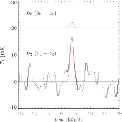
Figure 4: A model fit to the $\rho\,{\rm Oph\,A\,cloud}$, assumed to fill the Odin beam, with a column density of molecular hydrogen $N({\rm H}_{2})=2\times 10^{22}$ cm^-2 and a molecular oxygen abundance of $X({\rm O}_{2})=5\times 10^{-8}$. The results for both the 119 GHz and the 487 GHz (SWAS and Odin submm bands) lines are shown. According to this model, the 487 GHz line with $T_{\rm peak}=2$ mK is below detectability (see left-hand panel of Fig. 9).

The spectra in Figs. 2 and 4 show the O₂ emission integrated over the Odin beam of 10^′. Comparison with lines from other species ideally should be done at a comparable angular resolution. Pankonin & Walmsley (1978) observed $\rho\,{\rm Oph\,A}$ in a carbon recombination line (C $158\alpha$ at 1.6 GHz) with a beam of 7$\stackrel{{\scriptstyle\prime}}{{{}_{\bf\cdot}}}$8, close in size to that of Odin. Their beam-averaged $v_{\rm LSR}$ and $\Delta v_{\rm FWHM}$ were $3.15\pm 0.05$ km s^-1 and $1.43\pm 0.12$ km s^-1, respectively (see also Fig. 2). These values are again very close to the corresponding values of the O₂ line. In contrast to the methanol emission, this recombination radiation certainly originates in the PDR.

Based on the available observational evidence, it seems that no convincing conclusions regarding the location of the O₂ emission region can be drawn. The resolution to this problem would require the measurement of several O₂ transitions, a task which will likely be accomplished with the heterodyne instrument HIFI aboard Herschel, to be launched into space in the 2008 time frame.

5.4 The O₂ abundance

Of interest is the interpretation of these Odin observations in terms of the abundance of molecular oxygen, $X({\rm O}_{2})\equiv\int\!n({\rm O}_{2})\,dz/\!\!\int\!n({\rm H}_{2})\,dz=N({\rm O}_{2})/N({\rm H}_{2})$. Assuming optically thin line emission in thermodynamic equilibrium (for a discussion, see Liseau et al., 2005), the observed line intensity implies a column density $N({\rm O}_{2})=1\times 10^{15}$ cm^-2 (see Table 1). This calculation assumes a temperature of 30 K, a value which has been consistently obtained for both the gas (e.g., Loren et al., 1990) and the dust (Ristorcelli et al., 2007). The latter authors obtained $50^{\prime}\times 40^{\prime}$ maps in four FIR/submm wavebands, from 200 $\mu$m to 580 $\mu$m, using the balloon experiment PRONAOS (Pajot et al., 2006). The data provide constraints on the dust temperature and the spectral emissivity, which lead to maps of the dust optical depth. Assuming a total mass absorption coefficient of $5\times 10^{-3}$ cm² g^-1 at 1300 $\mu$m  with frequency dependence $\propto\nu^{2}$, the hydrogen column density is estimated to be $N({\rm H}_{2})=1\times 10^{22}$ cm^-2. This column density is at the low end of recent estimates, which were based on gas tracers (Pagani et al., 2003; Kulesa et al., 2005). Therefore, on the 10^′ scale ($10^{18}$ cm) of the Odin observations, an average value of $N({\rm H}_{2})=2\times 10^{22}$ cm^-2 is adopted here.

In conclusion, and acknowledging a factor of two uncertainty at least, the O₂ abundance in the $\rho\,{\rm Oph\,A\,cloud}$ is $X({\rm O}_{2})=5\times 10^{-8}$ (Fig. 4). With regard to model predictions (see Sect. 1), these results are consistent with either very young material of only a few times 10⁵ yr, which, given the ages of the stellar population, is unlikely, or more evolved gas at an age of some Myr to ten Myr, which requires careful ‘tuning’ in terms of selective desorption and/or specific grain-surface reactions, and thus appears unlikely, too. More distinct statements would need to include other chemical species in the analysis, which will be the subject of a forthcoming paper.

6 Conclusions

Below, we briefly summarize our main conclusions.

• Dedicated observations with Odin of the $\rho\,{\rm Oph\,A\,cloud}$ at 119 GHz have revealed a spectral feature at the frequency of the O₂ ($N_{J}=1_{1}-1_{0}$) transition.

• Both the center velocity and the width of this feature are consistent with other optically thin emission lines from $\rho\,{\rm Oph\,A}$.

• Analyzing the statistical properties of the noise essentially rules out the possibility that the O₂ feature is entirely due to noise in the observations.

• Specific reduction procedures have been applied to the data, which also helped to suppress any possible systematic effects.

• The significance of the line is more than $5\sigma$ and the beam-averaged O₂ abundance in the $\rho\,{\rm Oph\,A\,cloud}$ is $5\times 10^{-8}$.

Appendix A Data reduction

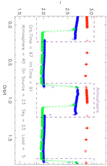
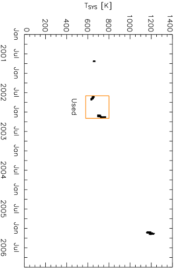
Figure 5: Selection procedure of usable data to be analysed - step 1. Left: The total power (in instrument units) during an orbit is shown. The colour coding is as follows: red = internal hot load (uppermost curve), blue = on source (intermediate) and green = sky measurement (lowest). The dashed rectangular boxes show the times of telluric atmosphere observations. Right: System noise temperature, $T_{\rm sys}$, during the four observing runs in 2001, 2002, 2003 and 2006, respectively. The red rectangular box identifies the selected data; 2001 data are of lower resolution and were, as such, excluded from the present analysis (but see: Pagani et al., 2003).

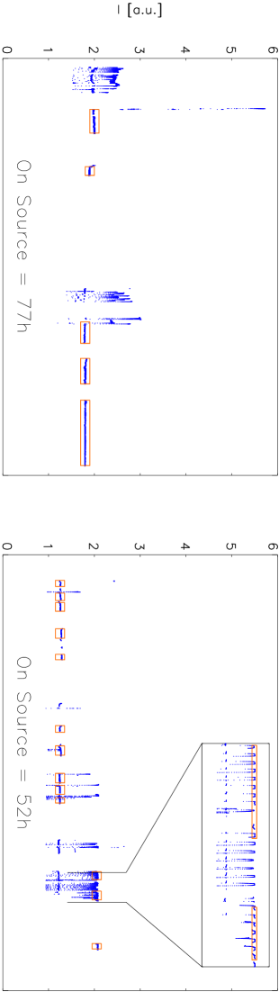
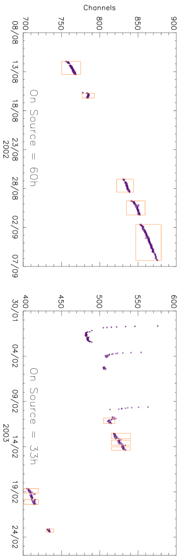
Figure 6: Selection procedure of usable data to be analysed. Displayed are data for 2002 and 2003. Top panels: Step 2. On-source raw total power data (in instrumental units). Red boxes include used data. Bottom panels: Step 3. Central spectrometer channel as function of the time for the all the data selected from the above criteria. Notice the change in scale, showing the long time drifts of the 119 GHz receiver. The jump in 2003 is due to the deliberate resetting of the spectrometer to keep the line near the center. Measurements of the frequency drift of the receiver were done for the data included in the boxes.

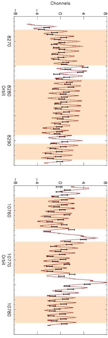
Figure 7: Frequency drift correlation with thermistor temperature (at the DRO). Upper panels: Measurement of the center channel for the 119 GHz oxygen line, when entering and leaving the Earth’s atmosphere, respectively. The red full-drawn line designates the inverse DRO-temperature, scaled in absolute level to the distribution of center channels, the assigned ‘error bars’ of which are $\pm 0.5$ channel widths. The shaded areas mark the selected data. Lower panels: As above, but for a single orbit. The shaded areas indicate the measurements of the center channel of the oxygen line for the entire passage of the Earth’s atmosphere. The hight of the shaded areas correspond to the error estimates of $\pm 0.5$ channel widths and the full-drawn line is the inverse DRO-temperature variation over the whole orbit.

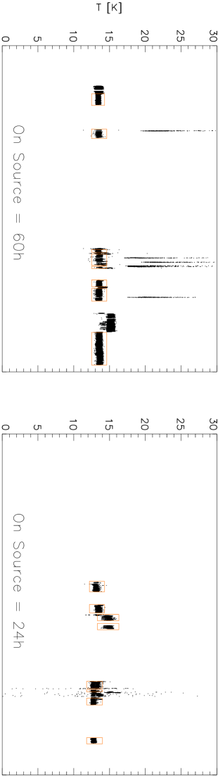
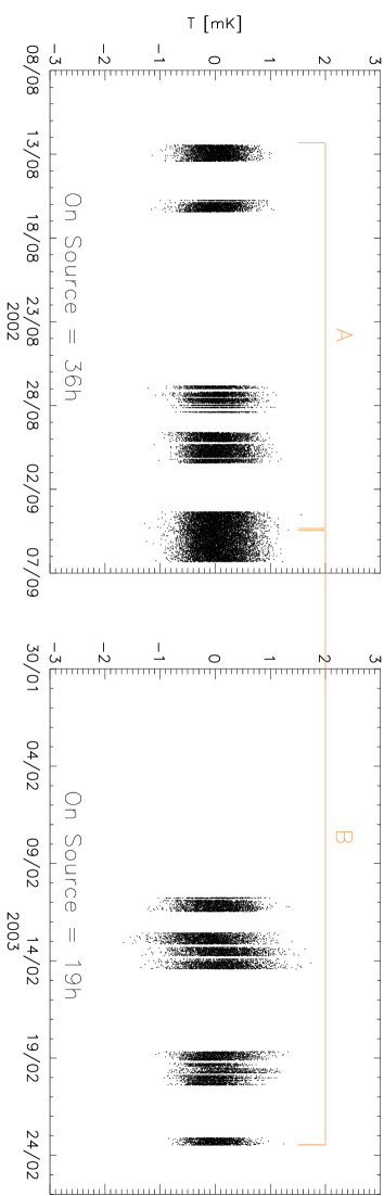
Figure 8: Selection procedure of usable data to be analysed - step 4. Top panel: On source calibrated data (mean power) Bottom panel: Final selected data after baseline removal. The bars, A and B, marks the division of the data set into two equal parts.

Except for a short period in the beginning of the Odin mission, the 119 GHz receiver has not been phase-locked. This has the consequence of both drifts in LO-frequency and stochastic variations in the amplifier gain. It is of imperative importance, therefore, that extreme care is exercised when reducing data which have been collected with this receiver and which are expected to be extremely weak. This is so in order not to create artificial signals nor to suppress faint real ones.

Odin has observed the $\rho\,{\rm Oph\,A\,cloud}$ at 119 GHz on four different occasions, viz. in 2001 (see: Pagani et al., 2003), in August 2002, in February 2003 and, finally, in February 2006. During the early observations (2001 and 2002) the system noise temperature was relatively stable, i.e. $T_{\rm sys}$ $\sim$ 650 K (Right panel in Fig. 5). When ‘left alone’ with the power on, the unlocked system is drifting towards lower frequencies in a nearly linear fashion. Eventually, the end of the receiver-band is approached, resulting in the increase of $T_{\rm sys}$. Consequently, in 2003, the system temperature had increased to 750 K. Even worse was the system behaving in 2006, when we attempted to support our earlier observations of the O₂ line by additional observations. At that stage, $T_{\rm sys}$ had risen to 1200 K, making these data essentially of nil value. In addition, the 2001 data were obtained at lower resolution and, therefore, the results presented in this paper are based only on the data collected during the 2002 and 2003 observing campaigns.

A.1 Selective data reduction

Because of the instability of the 119 GHz receiver, data collected with this instrument are of highly uneven quality. For this reason, a sizable fraction of the available data had to be abandoned. In the following, we identify and quantify the criteria which we applied for the selection of the useful data.

A.1.1 Gain stability

When observing with Odin, an astronomical object is blocked by the Earth during $\stackrel{{\scriptstyle>}}{{{}_{\sim}}}$ 1/3 of the orbit (left panel of Fig. 5). The observations were made in Dicke-switching mode, where the receiver alternates between the source and one of the sky beams and the internal hot load (Sect. 2. and Frisk et al., 2003; Olberg et al., 2003). For each orbit, the total integration time toward the source is therefore limited to 23 minutes. For the entire observing period, the total integration time for $\rho\,{\rm Oph\,A}$ was 136 hours, partitioned as 77 hr in 2002 and 59 hr in 2003, respectively.

In the top panels of Fig. 6, the uncalibrated on-source data are shown. From the figure, it is evident that the gain is not stable, but varies violently. Only data, for which the gain was stable or varied only slowly, were selected for further reduction. This reduced the integration times to 60 hr for 2002 and 33 hr for 2003.

A.1.2 Frequency drift correction

Odin ‘sees’ the Earth’s atmosphere for a third of an Odin revolution (left panel Fig. 5). Accurate frequency standards are thus provided by the telluric oxygen lines, viz. the $N_{J}=1_{1}-1_{0}$ line of O₂ and of its isotopic variant ${}^{16}{\rm O}^{18}{\rm O}$.

As discussed above, the frequency drift of the 119 GHz receiver with time is relatively linear - as long as the receiver stays powered on. This was essentially the case in the beginning of the Odin mission, when the 119 GHz receiver was almost always turned on. However, as outlined by Pagani et al. (2003), it became clear relatively soon that O₂ observations generally resulted in non-detections. Parallel 119 GHz observations became therefore essentially cancelled, with the aim to keep the O₂ line within the receiver band as long as possible.

Henceforth, the O₂ receiver was powered on only for times when a dedicated oxygen search was performed. However, initially (during the first few orbits) when the receiver is turned on, the drift is fast and highly non-linear (lower panels Fig. 6). As described by Larsson et al. (2003) for the 572 GHz receiver, this drift is temperature dependent.

A thermistor is placed at the Dielectric Resonator Oscillator (DRO). It has been established empirically that the frequency drift of the unlocked system correlates well with the temperature measured there (upper panel Fig. 7). During any given single orbit, the frequency variations should be small, however. This, in fact, has been confirmed by means of monitoring the atmospheric portion of the orbit, as is shown in the lower panels of Fig. 7.

With this good understanding of the behavior of the receiver and spectrum analyzer, the frequencies during the actual observations of the astronomical sources can be restored to high precision. We iterate here that the reliability of the reduction method had been demonstrated earlier by the successful reconstruction of the HC₃N ($J=13-12$) line at 118 270.7 MHz in a number of sources (e.g., for DR 21, see Hjalmarson et al., 2005). Although we had shown that our reduction method works well and reliably, none of the data with high drift rates (in the beginning of the observing periods in 2003) have, after all, been used in the present analysis (see boxes in the right lower panel of Fig. 6).

A.2 Final data selection

A.2.1 Baseline removal

The observations were done in Dicke-switching mode, alternating between the 10^′ main-beam, one of the 4$\stackrel{{\scriptstyle\circ}}{{{}_{\bf\cdot}}}$7 sky-beams (pointing off by $42$^∘), and the internal hot load. The calibrated signal, in the antenna temperature scale, is therefore given by

$$T_{\rm A}=\frac{I_{\rm On}-I_{\rm Sky}}{I_{\rm Load}-I_{\rm Sky}}=\frac{I_{\rm On}-I_{\rm Sky}}{I_{\rm Sky}}\times T_{\rm sys}\,\,.$$ (1)

On the basis of the observation of other optically thin lines, the O₂ line toward $\rho\,{\rm Oph\,A}$ is expected to be rather narrow. In order not to include possible artificial spectral features from the hot-load an average value around the line was used for the system noise temperature and adopted for the entire band, i.e.

$$T_{\rm sys}=\left<\frac{I_{\rm Sky}}{I_{\rm Load}-I_{\rm Sky}}\right>\,\,.$$ (2)

As back-end a digital autocorrelator (AC) was used. Using all 8 available correlator-chips gives a single band with resolution of 292 kHz (with channel separation = 125 kHz or 0.32 km s^-1) and bandwidth 100 MHz (corresponding to 250 km s^-1). The main beam and the sky-beams do not match perfectly, implying that the calibration results in a curvature over the band. An off-position, supposedly free of molecular emission, and 900^′′ north of $\rho\,{\rm Oph\,A}$ was also observed and these data could have been used to correct for the baseline residual. However, since the time spent on the off-position was much less than that spent on the on-position, the noise level in the difference spectrum would have been dominated by the observation of the off-position.

We resorted therefore to another method for the baseline removal. During the orbit about the Earth, the central Doppler-velocity of the line changes within the interval $-7$ km s^-1 to $+7$ km s^-1. Averaging over one or more orbits will therefore cause any narrow line to be smeared out. So for every observing period, a “super baseline” was constructed (and smoothed) and removed from every individual spectral scan during that period (bottom panels Fig. 8). This resulted finally in a useful integration time of 36 hr in 2002 and 19 hr in 2003 (47% and 32% of total on-time, respectively; see Sect. A.1.1).

Figure 9: Left: Noise temperature as a function of integration time ($t_{on}$): Thin and thick lines are for ideal rms noise for $T_{\rm sys}$ of 640 K (2002) and 720 K (2003), respectively and a resolution of 292 kHz. The dashed line refers to the expected rms-level of the 487 GHz line of O₂ (see the text and Fig. 4). Right: Autocorrelation of the finally reduced spectrum. Dotted line: before using a Hanning filter. Full line: after using a 3-channel-wide Hanning filter. Dashed line: the 292 kHz spectral resolution.

Figure 10: Final: The final spectrum ($T_{\rm A}$ in mK versus $v_{\rm LSR}$ in km s^-1). Besides the O₂ line near zero LSR-velocity, also another feature is discernable at about $+20$ km s^-1 (see the text). Hanning: The same spectrum after being smoothy by a Hanning filter (3 channels).

Figure 11: The finally reduced spectral data, which have been divided into two halves A and B (see lower panels in Fig. 8), showing the presence of the O₂ feature also at these reduced observing times.

A.2.2 Noise behaviour and presentation of spectra

In the left panel of Fig. 9, the rms noise of the finally selected data set is shown as a function of the integration time. The 119 GHz data follow the theoretical prediction for white noise reasonably well to the resolution of the spectrometer, 292 kHz or a little more then 2 channels (right panel Fig.  9). As a final reduction step the spectrum was passed through a Hanning filter of a 3-channel width to accommodate the resolution of the spectrometer. As seen in the right panel of Fig. 9 the result of this was that the effective resolution deteriorates to about 4 channels or 500 kHz.

The finally reduced data are shown in Fig. 10. The spectrum reveals two line features clearly above the noise level. These are the O₂ ($N_{J}=1_{1}-1_{0})$ line and a feature that coincides in frequency with c-C₂H₄O $(3_{2,\,2}-2_{1,\,1})$. In order to gauge the reality of these detections the data set was divided into two halves (Figs. 8 and 11). Obviously, the O₂ spectral feature is clearly seen in both spectra, lending further confidence to the reliability of the reduction method.

References

- Bergin et al. (2000) Bergin E.A., Melnick G.J., Stauffer J.R., et al., 2000, ApJ, 539, L 129
- Charnley et al. (2001) Charnley S.B., Rodgers S.D. & Ehrenfreund P., 2001, A&A, 378, 1024
- de Zeeuw et al. (1999) de Zeeuw P.T., Hoogerwerf R., de Bruijne J.H.J., Brown A.G.A. & Blaauw A., 1999, AJ, 117, 354
- Frisk et al. (2003) Frisk U., Hagström M., Ala-Laurinaho J., et al., 2003, A&A, 402, L 27
- Goldsmith et al. (2000) Goldsmith P.F., Melnick G.J., Bergin E.A., et al., 2000, ApJ, 539, L 123
- Goldsmith et al. (2002) Goldsmith P.F., Li D., Bergin E.A., et al., 2002, ApJ, 576, 814
- Hargreaves (2004) Hargreaves, T.L., 2004, M.Sc. thesis, McMaster University
- Hjalmarson et al. (2003) Hjalmarson Å., Frisk U., Olberg M., et al., 2003, A&A, 402, L 39
- Hjalmarson et al. (2005) Hjalmarson Å., Bergman P., Biver N., et al., 2005, Advan. Space Res., 36, p. 1031
- Ikeda et al. (2001) Ikeda M., Ohishi M., Nummelin A., et al., 2001, ApJ, 560, 792
- Kulesa et al. (2005) Kulesa C.A., Hungerford A.L., Walker C.K., et al., 2005, ApJ, 625, 19
- Larsson et al. (2003) Larsson B., Liseau R., Bergman P., et al., 2003, A&A, 402, L 69
- Larsson et al. (2005) Larsson B., et al., 2005, in: Protostars & Planets V, B. Reipurth, D. Jewitt & K. Keildited (eds.), LPI Contribution No. 1286, p. 8393
- Larsson et al. (2007) Larsson B., et al., 2007, in preparation
- Liseau et al. (1999) Liseau R., White G.J., Larsson B., et al., 1999, A&A, 344, 342
- Liseau et al. (2003) Liseau R., Larsson B., Brandeker A., et al., 2003, A&A, 402, L 73
- Liseau et al. (2005) Liseau R., et al., 2005, in: IAU Symposium 231, Recent Successes and Current Challenges, D.C. Lis, G.A. Blake & E. Herbst (eds.), p. 301 (see also: astro-ph/0509589)
- Loren et al. (1990) Loren R.B., Wootten A. & Wilking B.A., 1990, ApJ, 365, 269
- Maréchal et al. (1997) Maréchal, P., Pagani, L., Langer, W.D. & Castets, A., 1997, A&A, 318, 252
- Olberg et al. (2003) Olberg M., Frisk U., Lecacheux A., et al., 2003, A&A, 402, L 35
- Olofsson et al. (1998) Olofsson G., Pagani L., Tauber J., et al., 1998, A&A, 339, L 81O
- Pagani et al. (2003) Pagani L., Olofsson A.O.H., Bergman P., et al., 2003, A&A, 402, L 77
- Pajot et al. (2006) Pajot F., Stepnik B., Lamarre J.-M., et al., 2006, A&A, 447, 769
- Pan et al. (1998) Pan J., Albert S., Sastry K.V.L.N., et al., 1998, ApJ, 499, 517
- Pankonin & Walmsley (1978) Pankonin V. & Walmsley C.M., 1978, A&A, 64, 333
- Ristorcelli et al. (2007) Ristorcelli I., et al., 2007, in preparation
- Roberts & Herbst (2002) Roberts H. & Herbst E., 2002, A&A, 395, 233
- Spaans & van Dishoeck (2001) Spaans M. & van Dishoeck E.F., 2001, ApJ, 548, L 217
- Viti et al. (2001) Viti S., Roueff E., Hartquist T.W., Pineau des Forêts G. & Williams D.A., 2001, A&A, 370, 557
- Willacy et al. (2002) Willacy K., Langer W.D. & Allen M., 2002, ApJ, 573, L 119
- Wilson et al. (1999) Wilson C.D., Avery L.W., Fich M., et al., 1999, ApJ, 513, L 139