Phase models of the Milky Way stellar disc

Abstract

We present a new iterative method for constructing equilibrium phase models of stellar systems. Importantly, this method can provide phase models with arbitrary mass distributions. The method is based on the following principle. Our task is to generate an equilibrium $N$-body system with a given mass distribution. For this purpose, we let the system reach equilibrium through its dynamical evolution. During this evolution we hold mass distribution in this system. This principle is realized in our method by means of an iterative procedure. We have used our method to construct a phase model of the disc of our Galaxy. In our method, we use the mass distribution in the Galaxy as input data. Here we used two Galactic density models (suggested by Flynn, Sommer-Larsen & Christensen 1996; Dehnen & Binney 1998a). For a fixed-mass model of the Galaxy we can construct a one-parameter family of equilibrium models of the Galactic disc. We can, however, choose a unique model using local kinematic parameters that are known from Hipparcos data. We show that the phase models constructed using our method are close to equilibrium. The problem of uniqueness for our models is discussed, and we discuss some further applications of our method.

1 Introduction

The construction of equilibrium phase models of galaxies is an important area of research in galactic astronomy. Such models are of interest from a number of points of view. They are important for understanding the dynamics of galaxies, and they are necessary for defining the initial conditions in $N$-body models of stellar systems.

In this paper, we consider the problem of constructing an equilibrium model of the stellar disc of a spiral galaxy. Our purpose is to construct a phase model of the Galactic stellar disc. Various approaches to solving this problem have been suggested (see, for example, the review in Rodionov & Sotnikova 2006, hereafter RS06).

The first approach is based on Jeans equations (equations for moments of the equilibrium velocity distribution function). One such method of constructing equilibrium disc models was described by Hernquist (1993). An advantage of this method is its relative simplicity. It is applicable for a stellar disc with an arbitrary density profile and any external potential. It has, however, a significant drawback. The system of Jeans equations used is not closed, so it is necessary to introduce an additional condition in order to close it. As a result, the constructed model is often far from equilibrium, as we showed when we used the closure condition suggested by Hernquist (1993). A more detailed critical analysis of this method is given in RS06.

The second approach is based on Jeans theorem, according to which any function of motion integrals is a solution of the stationary collisionless Boltzmann equation (see, for example, Binney & Tremaine 1987); that is, it is an equilibrium distribution function. There is, however, one significant disadvantage of such an approach to constructing a three-dimensional equilibrium model of a stellar disc. Two integrals of motion are well known for axisymmetric models: $E$ is energy and $L_{z}$ is the angular momentum about the symmetry axis. However, for systems having phase density $f(E,\,L_{z})$, the dispersions of the residual velocities in the radial and vertical directions have to be the same, which is in disagreement with observations of spiral galaxies, in particular for the solar neighbourhood (see, for example, Dehnen & Binney 1998b). Axisymmetric models with different velocity dispersions in the radial and vertical directions may be constructed if the phase density depends on three integrals of motion $f(E,\,L_{z},\,I_{3})$, where $I_{3}$ is the third integral of motion. However, an expression for the third integral is not known for the general case. It is possible to use the energy in vertical oscillations as the third integral when the residual velocities are much lower than the rotation velocity with respect to the symmetry axis (cold thin disc). In such a way, one can construct models of approximately exponential stellar discs, as done, for example, by Kuijken & Dubinski (1995); Widrow & Dubinski (2005). These authors also describe the procedure of phase density construction for multicomponent models of disc galaxies.

One further original method for constructing phase galactic models was developed by Schwarzschild (1979). In this method, it is assumed that the total galactic potential is known. A large number of orbits (library of orbits) in this potential are constructed, and a model consisting of the particles placed on these orbits is constructed in such a way that the resulting model has an initial density profile. We note that this approach is similar to our Orbit.NB method described below.

In this paper, we use a new iterative method proposed in RS06. In RS06, the iterative method was applied to construct a model of the stellar disc of a spiral galaxy (the problem under consideration). In our notation, this realization of the iterative method is termed Nbody.SCH. It has, however, a number of disadvantages. The Nbody.SCH method has a problem with the construction of a relatively cold stellar disc: using the Nbody.SCH method it is not possible to construct a sufficiently cold equilibrium stellar disc. The stellar disc of our Galaxy is rather cold. The model of the stellar disc of our Galaxy constructed using the Nbody.SCH method is notably far from equilibrium. Moreover, the Nbody.SCH method cannot be directly applied to a stellar system with arbitrary geometry (for example, it cannot be applied to elliptical galaxies).

The first objective of our work is to develop a new realization of the iterative method without the disadvantages of the Nbody.SCH approach. The second objective is to construct a phase model of the Galactic disc using this new method.

Using the iterative method we can construct a phase model of a stellar system with a given mass distribution. Therefore, in order to construct a phase model of the Galactic disc we need the mass distribution of the Galaxy. A number of density models for the Milky Way Galaxy have been constructed. We use only two of them (see Flynn, Sommer-Larsen & Christensen 1996; Dehnen & Binney 1998a).

The density models used are described in Section 2. In Section 3 we present the iterative method and its modifications. Two versions of the iterative method are considered in detail. In our notation, these methods are called Orbit.NB and Nbody.NB. The Orbit.NB method gives fairly specific and probably non-physical models. Although such models are probably non-physical, the fact that such equilibrium models exist is of interest. It gives some insight into the problem of uniqueness of phase models of the stellar disc. The models constructed by the Orbit.NB method are discussed in Section 4. We think that the models constructed by Nbody.NB method are physical. In Section 5 we present phase models for the Galactic disc constructed using this method. It is important, that Nbody.NB solves the first objective of our work (see above). A summary of the results is given in Section 6, wherein we also discuss further applications of our method and models.

2 Galactic density models

There are many Galactic density models in the literature. We have chosen two of them (see Flynn, Sommer-Larsen & Christensen 1996; Dehnen & Binney 1998a). We note that Dehnen & Binney (1998a) presented a whole family of density models. We have chosen the model ‘2’ from this paper. Both models under consideration are axisymmetric.

Let us briefly outline the models used.

2.1 Model of Flynn, Sommer-Larsen & Christensen (1996)

This model contains three main components: a dark halo, central component, and disc. For the dark halo, the authors used a logarithmic potential (see Binney & Tremaine 1987, p. 46):

$$\Phi_{H}(R,z)=\frac{1}{2}V_{H}^{2}\ln(r^{2}+r_{H}^{2})\,,$$ (1)

where $V_{H}$ and $r_{H}$ are the halo parameters (circular velocity at large $r$ and halo scalelength), $R$ is the cylindrical radius, $r=\sqrt{R^{2}+z^{2}}$ is the spherical radius.

The central component consists of two spherical subsystems. The first one represents the bulge$+$stellar halo; the second one is the inner core of the Galaxy. Each component is approximated by a Plummer sphere (see Binney & Tremaine 1987, p. 42–43). The expression for the whole potential of the central component has the form

$$\Phi_{C}(R,z)=-\frac{GM_{C_{1}}}{\sqrt{r^{2}+{r_{C_{1}}}^{2}}}-\frac{GM_{C_{2}}}{\sqrt{r^{2}+{r_{C_{2}}}^{2}}}\,,$$ (2)

where $G$ is the gravitational constant; $M_{C_{1}}$ and $r_{C_{1}}$ are the mass and scalelength for the first subsystem; and $M_{C_{2}}$ and $r_{C_{2}}$ are the same parameters for the second.

The disc in this model is the superposition of three Miyamoto & Nagai (1975) discs. The whole disc potential has the form

$$\Phi_{D}(R,z)=-\sum_{n=1}^{3}\frac{GM_{D_{n}}}{\sqrt{R^{2}+(a_{n}+\sqrt{z^{2}+b^{2}})^{2}}}\,.$$ (3)

Here, $b$ is the disc scaleheight (which is the same for all three components); the parameters $a_{n}$ are the disc scalelengths; and the values $M_{D_{n}}$ are the masses of the disc components.

Flynn, Sommer-Larsen & Christensen (1996) have suggested the following values for the above parameters:

$r_{H}=8.5$ kpc, $V_{H}=210$ km s^-1,
$r_{C_{1}}=2.7$ kpc, $M_{C_{1}}=3.0\cdot 10^{9}$ $M_{\odot}$,
$r_{C_{2}}=0.42$ kpc, $M_{C_{2}}=1.6\cdot 10^{10}$ $M_{\odot}$,
$b=0.3$ kpc,
$M_{D_{1}}=6.6\cdot 10^{10}$ $M_{\odot}$, $a_{1}=5.81$ kpc,
$M_{D_{2}}=-2.9\cdot 10^{10}$ $M_{\odot}$, $a_{2}=17.43$ kpc,
$M_{D_{3}}=3.3\cdot 10^{9}$ $M_{\odot}$, $a_{3}=34.86$ kpc.

Table 1 in Flynn, Sommer-Larsen & Christensen (1996) contains a small misprint: instead of $V_{H}=220$ km s^-1 it should be $V_{H}=210$ km s^-1 (Flynn, private communication). We note that one of the disc components ($n=2$) has a negative density; however, the total density in the disc is positive, and the model is therefore physical. Over a large range in $R$, the disc density profile is approximately exponential, with a scalelength of approximately 4 kpc. This is possibly an overestimated value (Flynn, private communication). Hereafter, we will refer to this model as FSLC. Fig. 1 shows the dependences of cumulative masses $M(r)$ and circular velocity curves for the whole FSLC model, for all components without the disc, and for the disc only.

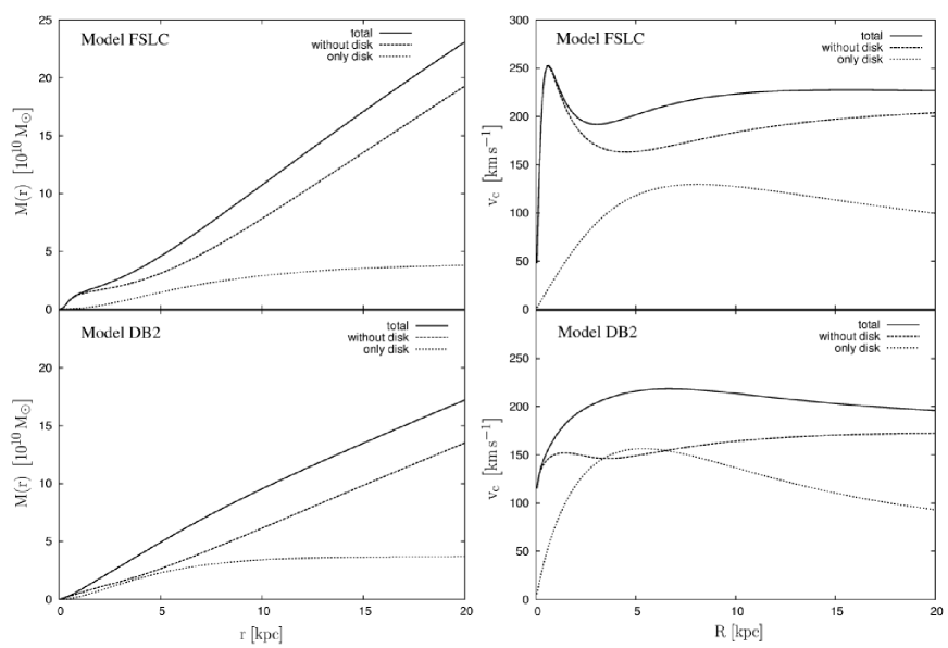
Figure 1: The dependence of cumulative masses on radius (left panels) and the circular velocity curves (right panels) for various components in the density models FSLC and DB2. Here the cumulative mass $M(r)$ is the mass inside the sphere of radius $r$. Solid lines show the dependences for a whole model; long-dashed lines correspond to the whole model without the disc; and short-dashed lines correspond to the stellar disc only. We use the thin stellar disc in the DB2 model as the stellar disc.

2.2 Model of Dehnen & Binney (1998a)

In addition to the FSLC model, we consider one model of the family suggested by Dehnen & Binney (1998a). Every model of this family consists of five components. There are three disc components (interstellar medium (ISM), thin stellar disc, and thick stellar disc) and two spheroidal components (dark halo and bulge).

The distribution of volume density in each disc component has the form

$$\rho_{d}(R,z)=\frac{\Sigma_{d}}{2z_{d}}\exp\biggl{(}-\frac{R_{m}}{R_{d}}-\frac{R}{R_{d}}-\frac{|z|}{z_{d}}\biggr{)}.$$ (4)

Here $\Sigma_{d}$ is the central surface density of the component, and parameters $R_{d}$ and $z_{d}$ give scalelength and scaleheight of the component. By using the parameter $R_{m}$ one can introduce a central density depression in the disk.

The density distribution for each spheroidal component has the form

$$\rho_{s}(m)=\rho_{0}\biggl{(}\frac{m}{r_{0}}\biggr{)}^{-\gamma}\biggl{(}1+\frac{m}{r_{0}}\biggr{)}^{\gamma-\beta}\exp{(-m^{2}/r_{t}^{2})},$$ (5)

where

$$m=\sqrt{R^{2}+q^{-2}z^{2}}.$$ (6)

Here $\rho_{0}$, $r_{0}$, $\gamma$, $\beta$, $q$, $r_{t}$ are the parameters of the spheroidal components.

We use model 2 from this paper, hereafter the DB2 model. This choice is somewhat arbitrary. We do not consider other models from this paper because a comparison of the different Galactic models is outwith the goals of this paper. The parameters of the DB2 model are shown in Tables 1 and 2. The details of the construction of this model are given in Dehnen & Binney (1998a).

Table 1: Parameters for three disk components in the DB2 model.

comp.	$\Sigma_{d},\;{\rm M_{\odot}\,pc^{-2}}$	$R_{d},\;{\rm kpc}$	$R_{m},\;{\rm kpc}$	$z_{d},\;{\rm kpc}$
thin disk	1022	2.4	0	0.18
thick disk	73.03	2.4	0	1
ISM	113.6	4.8	4	0.04

Table 2: Parameters for the two spheroidal components in the DB2 model.

comp.	$\rho_{0},\;{\rm M_{\odot}\,pc^{-3}}$	$r_{0},\;{\rm kpc}$	$\gamma$	$\beta$	$q$	$r_{t},\;{\rm kpc}$
bulge	0.7561	1	1.8	1.8	0.6	1.9
halo	1.263	1.090	-2	2.207	0.8	$\infty$

Here we construct an equilibrium $N$-body model of the stellar Galactic disc. As the stellar disc, we take only the thin stellar disc from the DB2 model. The construction of a two-component stellar disc in this model will be the subject of future investigations.

In addition to the density, we need to calculate the potentials of the various components in the DB2 model. The potentials were numerically calculated using the code GALPOT by Walter Dehnen. The method of potential determination is described in (Dehnen & Binney, 1998a). The code was taken from the NEMO package (http://astro.udm.edu/nemo; Teuben 1995).

The cumulative mass profile $M(r)$ and circular velocity curve for the DB2 model are shown in Fig. 1 for the whole model, for all components apart from the thin stellar disc, and for the thin stellar disc only.

Fig. 1 shows that the FSLC and DB2 models are different. The FSLC model has a more massive and concentrated bulge with respect to the DB2 model. In particular, this massive bulge is the reason for the central peak in the rotation curve for the FSLC model. Furthermore, the relative disc contribution in the whole mass and the circular velocity curve for the inner model ($R\leq 8\,{\rm kpc}$) is significantly higher in the DB2 model than in the FSLC model.

3 Iterative method for equilibrium models constructing

3.1 Basic idea of iterative method

The iterative method is used to construct $N$-body models close to equilibrium and with a given mass distribution (see RS06 for details). The basic idea of this approach is as follows. First, we generate an $N$-body system with a given mass distribution but with arbitrary initial particle velocities (which, for example, can be taken as zero). Furthermore, we let the system reach equilibrium through its dynamical evolution. During this evolution we hold mass distribution in the system. If necessary, some parameters of the velocity distribution can be fixed. This is achieved in the following way.

The general algorithm of the iterative method is as follows.

1. An N-body system with a given mass distribution but with arbitrary particle velocities is constructed. The velocities can, for example, be taken to be zero.

2. The system is evolved on a short time-scale.

3. We construct a new N-body system, with the same given mass distribution but with velocities chosen according to the velocity distribution in the system already evolved. We note that, if there are some limitations on the velocity distribution, this distribution should be corrected taking into account these restrictions (see the discussion below).

4. We return to point 2. We repeat such cycles until the velocity distribution stops changing.

As a result, we obtain an $N$-body model close to equilibrium that has a given density profile (see RS06 and our results below for details).

We can discuss the iterative approach in a more general manner. When one needs to find an equilibrium state of an arbitrary dynamical system, but so that this state has some necessary properties (in the case under study, the dynamical system is a set of gravitating points and the necessary property is the density profile), one can simply give a possibility for the system itself to tune to the equilibrium state, holding the necessary parameters.

The idea of our iterative method is simple. Its realization in practice is more complicated. The main difficulty is the third stage, when it is necessary to construct a model with the same velocity distribution as the evolved model from the previous iteration step.

Below we discuss an application of the iterative procedure to the problem of constructing an equilibrium model of the Galactic disc.

3.2 Equilibrium models of stellar disks

3.2.1 Family of equilibrium models

Our task is to construct an equilibrium model of the stellar disc of our Galaxy. We consider all Galactic components as axisymmetric, and can formulate our task in the following way. We need to construct an equilibrium $N$-body model of a stellar disc with a fixed density distribution $\rho_{\rm disk}(R,z)$ that is embedded in the rigid external potential $\Phi_{\rm ext}(R,z)$, where $\Phi_{\rm ext}(R,z)$ is created by all Galactic components except the stellar disc (i.e. the dark halo and bulge).

It can be expected that at least a one-parameter family of equilibrium models will exist when the functions $\rho_{\rm disk}(R,z)$ and $\Phi_{\rm ext}(R,z)$ are fixed. The parameter of this family is the fraction of kinetic energy contained in the residual motions.

The reason why this family exists is as follows. It is possible to show that, if $\rho_{\rm disk}(R,z)$ and $\Phi_{\rm ext}(R,z)$ are fixed, then for all equilibrium discs the total kinetic energy should be the same. This is a direct consequence of the virial theorem. This kinetic energy can, however, be distributed between regular rotation and residual velocities in different manners. Cold equilibrium models exist when a large fraction of the kinetic energy is concentrated in the regular rotation (an extreme case is the model with circular orbits), and hot equilibrium models exist when a large fraction of the kinetic energy is concentrated in the residual motions.

In RS06, the authors showed that, for exponential disc, a one-parameter family of models can be constructed by the iterative method for fixed $\rho_{\rm disk}(R,z)$ and $\Phi_{\rm ext}(R,z)$. If the iterations are started from different initial states, different models result; however, they all form a one-parameter family. As expected, the parameter is the fraction of kinetic energy concentrated in the residual motions. In order to obtain a definite model from this one-parameter family, the method suggested in RS06 can be used. We simply fix the fraction of kinetic energy during the iterative process. In principle, we could fix any value characterizing the “heat” degree of the disc. The authors of RS06 suggest using the value of angular momentum about the $z$-axis (symmetry axis) as this parameter:

$$L_{z}=\sum_{i=1}^{N}m_{i}v_{\varphi i}R_{i}\,,$$ (7)

where $m_{i}$, $v_{\varphi i}$, $R_{i}$ are the mass, azimuthal velocity, and cylindrical radius of the $i$-th particle.

We fix the value of $L_{z}$ at each iteration step. When we have constructed a new model (which has the same velocity distribution as the slightly evolved model from the previous iteration step), we correct the azimuthal velocities so that the total angular momentum of the system is the same as the fixed value of $L_{z}$ . This is done as follows. Let $L_{z}$ be this fixed angular momentum, and let $L_{z}^{\prime}$ be the current value of the angular momentum. The new azimuthal velocities of particles are prescribed as follows:

$$v_{\varphi i}=v_{\varphi i}^{\prime}+\frac{(L_{z}-L_{z}^{\prime})}{{\sum_{j=1}^{N}R_{j}m_{j}}}\,,$$ (8)

where $v_{\varphi i}^{\prime}$ is the current value of the azimuthal velocity of the $i$-th particle, and $v_{\varphi i}$ is the corrected azimuthal velocity of the $i$-th particle.

We note that by using the iterative method with fixed $L_{z}$, one can construct colder models with respect to the ones without $L_{z}$ fixed (because the cold stellar disc tends to heating during the dynamical evolution). The stellar disc of the Galaxy is rather cold. Thus it is difficult to construct a cold model of the Galactic disc without fixing $L_{z}$. We therefore fix $L_{z}$ in all our models.

3.2.2 Variants of the velocity distribution “transfer”

We first discuss the core of the iterative method, namely an algorithm to transfer the velocity distribution (item 3 in the iterative procedure).

The transfer problem is as follows. We have an “old” model. This is an evolved model from the previous iteration step from which we would like to copy a velocity distribution. Moreover, we have a “new” model that is constructed according to the fixed density distribution. We have to give the velocities to the particles in the new model using the velocity distribution in the old model. How do we do this?

In RS06, the authors used an algorithm of velocity distribution “transfer”, which is based on assuming that the particles have a truncated Schwarzschild velocity distribution. We describe this approach briefly. We take a disc model (old model) from which we are going to “copy” the velocity distribution. The model is divided along the $R$-axis into various regions (concentric cylindrical tubes). For each region, we calculate four velocity distribution moments ($\bar{v}_{\varphi}$, $\sigma_{R}$, $\sigma_{\varphi}$, $\sigma_{z}$ — the mean azimuthal velocity and three dispersions of residual velocities along the directions $R$, $\varphi$, and $z$). These moments are used for the velocity choice in the new model. We assume that the velocity distribution is the Schwarzschild one, but without the particles that can go out of the disc (see RS06 for details).

We slightly modified this scheme of velocity transfer. The model is divided into regions not only along the $R$-axis, but also along the $z$-axis. The regions are chosen in such a way that they all contain similar numbers of particles.

This method of velocity distribution transfer has, however, two drawbacks (even in its modified form). First, an a priori assumption is made that the velocity distribution is the Schwarzschild one. Second (and more importantly), this method cannot be used for other geometry systems (e.g. triaxial elliptical galaxies).

We have developed another method of velocity distribution transfer. We believe that it is a more general and simpler method. The basic idea of this new method is as follows. We prescribe to the new-model particles the velocities of those particles from the old model that are nearest to the ones in the new model.

The simplest (although not quite successful, as we show below) implementation of this idea is evident. One can prescribe to each particle in the new model the velocity of the nearest particle from the old model. Let us formulate this proposition more strictly. For each $i$th particle from the new model, one finds the old-model $j$th particle with the minimum value of $|{\bf r}^{new}_{i}-{\bf r}^{old}_{j}|$. Here, ${\bf r}^{new}_{i}$ is the radius vector of the $i$th particle in the new model, and ${\bf r}^{old}_{j}$ is the radius vector of the $j$th particle in the old model. One then takes as the velocity of the $i$th particle in the new model the velocity of the $j$th particle in the old model.

This simple algorithm has, however, one essential problem. If the numbers of particles in the old and new models are the same then only about one-half of the particles in the old model participate in the velocity transfer. The reason is that many old-model particles have a few particles in the new model to which they transfer their velocities. At the same time, almost one-half of the particles in the old model do not transfer their velocities at all. This means that a significant amount of information on the velocity distribution will be lost in the transfer process. The noise will therefore grow, and this is indeed observed in numerical simulations. Thus, one cannot construct an $N$-body model close to equilibrium by the iterative method described above using this transfer algorithm.

It is, however, possible to modify the transfer scheme in order to overcome this failure. An input parameter of this improved algorithm is the “number of neighbours” $n_{nb}$ . For each particle in the old model, we introduce the parameter $n_{use}$, which denotes the number of times this particle is used for velocity copying. At the beginning of the transfer procedure, we assume $n_{use}=0$ for each particle in the old model. We then consider all particles in the new model. For each particle from the new model, we find the nearest $n_{nb}$ neighbours in the old model (in this case, the closeness is understood as the minimum distance between the particles in the old model and the point at which the particle of interest from the new model is placed). We then reveal a subgroup of particles that have a minimum $n_{use}$ among these $n_{nb}$ neighbours, and among this subgroup we find the particle that is the closest one to the position of the new-model particle. We prescribe to the new-model particle the velocity of the found particle from the old model. Moreover, we add one to the parameter $n_{use}$ of this old-model particle.

We note that this algorithm is the same as the previous one if $n_{nb}=1$. As mentioned above, the problem with this algorithm is that only one-half of the particles take part in the velocity distribution transfer. If we take $n_{nb}=10$, only a small fraction (a few per cent) of old-model particles do not take part in the transfer process. Using this improved transfer method in the iterative procedure gives good results in the sense that the constructed models are close to equilibrium.

In this method, one can take into account that the galactic models under study are axisymmetric. One just has to redefine the distance between the particles. That is, one can search for the nearest particles in two-dimensional space $Rz$ instead of three-dimensional space $XYZ$. In this case, one should transfer the velocities in cylindrical coordinates in order to remove any dependence on the azimuthal angle. This guarantees that the constructed model has an axisymmetric velocity distribution. We use this method when constructing the model of the Galactic stellar disc (see below).

We note that this method of velocity transfer is universal, and can be applied in systems with arbitrary geometry. The models constructed in this way are close to equilibrium, but, partly because of this, the method has a small disadvantage. The iterations converge much more slowly than the ones in the above-mentioned method based on the Schwarzschild velocity distribution. The reason for this slow convergence is that even intermediate models are fairly close to equilibrium, so that the models change only slightly over one iteration, and the iterations converge slowly.

3.2.3 Different ways of system evolution simulations

We discuss one more way to modify the iterative method. In the general algorithm of the iterative procedure, item 2 allows the model to evolve over a short time-scale. This means that one needs to simulate the self-consistent $N$-body evolution of the stellar disc during a short time in the field of the external potential $\Phi_{\rm ext}$. There is, however, another possibility. Instead of simulating the self-consistent dynamical evolution of the $N$-body system, one can simulate the motions of $N$ massless test particles in the regular galactic potential $\Phi_{\rm disk}+\Phi_{\rm ext}$, where $\Phi_{\rm disk}$ is the disc potential corresponding to the density $\rho_{\rm disk}$. We note that the simulation of a system of $N$ test particles in a rigid potential is much less cumbersome than simulation of the self-consistent $N$-body system.

At first glance, both methods have to give practically the same results, because the initial stellar disc has the density profile $\rho_{\rm disk}$ that creates the potential $\Phi_{\rm disk}$. It is expected that the iterations will converge to an equilibrium state. Therefore in the self-consistent case, the disc at the late stages of the iterative process will be close to equilibrium and will not significantly change its density profile during a single iteration (especially because we follow the evolution over a short time-scale).

However, the iterative methods using these two modes of calculation may lead to essentially different results (see below).

3.2.4 Comparison of different realizations of iterative method

We thus have two ways to perform the velocity distribution transfer. The first one is based on calculations of the velocity distribution moments and assumes a Schwarzschild velocity distribution (hereafter we refer to this method as SCH). The second is based on prescribing to the particles in the new model the velocities of the nearest particles in the old model (hereafter we refer to this method as NB).

We also have two ways of performing system simulations. The first one is the self-consistent simulation of the N-body gravitating system evolution (hereafter we refer to this approach as Nbody). The second is the calculation of massless particle orbits in the regular potential $\Phi_{\rm disk}+\Phi_{\rm ext}$ (hereafter we refer to this approach as Orbit).

We thus have four versions of the iterative method: Nbody.SCH, Nbody.NB, Orbit.SCH, and Orbit.NB. Our task is to choose from among them the method that will be used to construct a phase model of the Galactic stellar disc.

We will show in Section 4 that the Orbit.NB approach gives models that are probably non-physical. However, the very fact of the existence of such “strange” equilibrium models is of interest, and gives food for thought (see Section 4 for details).

We thus need to choose from among three approaches: Nbody.NB, Nbody.SCH, and Orbit.SCH. Our test simulations have shown the following. The models of hot discs constructed by all these approaches are similar. The only exception is that the models constructed by the Nbody.NB method are slightly closer to equilibrium. However, the models of cold discs are significantly different. In particular, this concerns models of the Galactic disc, because the Galactic disc is rather cold. The models of cold discs constructed with the Nbody.NB approach are close to equilibrium, whereas the ones constructed with the Orbit.SCH and Nbody.SCH approaches are quite far from equilibrium. We can therefore conclude that the Orbit.SCH and Nbody.SCH approaches are not suitable for constructing equilibrium models of cold stellar discs. Moreover, from a methodical point of view, it is more correct to use the NB transfer approach, because here we do not make any a priori assumptions concerning the form of the velocity distribution (in contrast to the SCH method).

We shall thus use the Nbody.NB approach to construct phase models of the Galactic stellar disc (see Section 5).

3.2.5 Technical comments

We note a few important technical details.

In the iterative method, there is one parameter — the time interval $t_{i}$ of each iteration. This is the time interval over which the system evolves during each iteration. How do we choose the value of $t_{i}$? This time should not be too short, because in this case the system would have no time to evolve during one iteration step. On the other hand, it should not be too long. At least, this time should be much shorter than the typical times of development of various instabilities; otherwise, these instabilities may change the system substantially. We cannot suggest any strict criterion for choosing $t_{i}$. We have chosen a value from numerical simulations. Our simulations have shown that, if we take $t_{i}$ within reasonable limits (not too short and not too long), the constructed models are the same (within the noise limits). Of course, this is valid only when we use the model with the same $L_{z}$ (see Section 3.2.1). In any case, a basic test of every method to construct the equilibrium models would be a numerical check that the model is close to equilibrium.

We have used the following modification of the iterative method in several simulations. We do not take a fixed iteration time, but choose this time randomly within the range $(0,\,t^{\rm max}_{i})$. If one makes the iterations with the fixed $t_{i}$, the following situation may occur in principle. The iterations could converge to an artificial non-equilibrium state when the model has large changes at intermediate times within one iteration, however in the end of iteration, it could have the same state as in the beginning of the iteration. Another situation that could occur is that the model could jump from one state to another, i.e. oscillations between two states occur. The random choice of the iteration step enables us to avoid such situations. However, if we consider the Nbody.NB approach, fixed and random iteration steps give practically the same models as output.

In many of our simulations, we used the following method to decrease the CPU time. Initially, we make the iterations have a low accuracy (for example by using a smaller number $N$ of bodies) and then gradually increase the accuracy up to a pre-defined limit. This scheme was used in all simulations of Section 5.

In all our $N$-body simulations (self-consistent scheme), we used the TREE code (Barnes & Hut, 1986) and a few other codes from the NEMO package (http://www.astro.umd.edu/nemo; Teuben 1995). We used our original codes to simulate the motions of particles in the rigid potential.

4 Non-physical models. hypothesis of uniqueness

4.1 Models constructed with the Orbit.NB approach

In this section we consider the models constructed with the Orbit.NB approach. We will show that these models are probably non-physical models. However, the very fact of the existence of such models is of interest. It gives some insight into the problem of uniqueness of phase models of the stellar disc.

One noteworthy feature of the iterative Orbit.NB approach is that usually at fixed $\rho_{\rm disk}(R,z)$, $\Phi_{\rm ext}(R,z)$, and $L_{z}$ essentially different models can be constructed by means of this approach, although all other versions of the iterative method give similar (within the limits of noise) final models at a fixed value of $L_{z}$. Another important feature of this approach is that the velocity distributions of the final models are very different from the Schwarzschild distribution. We consider this fact in more detail below.

Let us consider a model constructed by the Orbit.NB approach. We take the FSLC density model (see Section 2.1); that is, the disc density $\rho_{\rm disk}$ is taken from the FSLC model, and the rigid potential $\Phi_{\rm ext}$ is generated by all FSLC model components except the disc. The disc density is taken to be zero at $R>R_{\rm max}=30\;\rm kpc$ or $|z|>z_{\rm max}=10\;\rm kpc$. We take the cold initial model in which all particles move along circular orbits. We used 1000 iterations for $N=200,000$, and then 100 iterations for $N=500,000$. The integration step was taken as $dt=0.5\;\rm Myr$. The number of neighbours for the velocity distribution transfer was taken to be $n_{\rm nb}=100$. We used a scheme with randomized iteration time (see Section 3.2.5) with $t_{i}^{\rm max}=100\;\rm Myr$. During the iterative process, we fixed the angular momentum as $L_{z}=6.412\cdot 10^{13}\;M_{\odot}\>\rm kpc\>km\>s^{-1}$. We note that in all simulations the following system of units was used: gravity constant $G=1$, length unit $u_{r}=1\;\rm kpc$, time unit $u_{t}=1\;\rm Myr$. In this system of units, the chosen value is $L_{z}=0.295$ (hereafter we indicate the parameter $L_{z}$ in this system of units). We refer to this model as FSLC.O. We consider only this model; however, we emphasize that very different models may be constructed by the Orbit.NB approach at fixed $L_{z}$ if we take different initial models.

In addition to the constructed FSLC.O model, we consider its changes during further dynamical evolution (self-consistent $N$-body evolution of the constructed stellar disc in the field of the external potential $\Phi_{\rm ext}$). The parameters of simulation are taken as follows: number of bodies $N=100\,000$, integration time step $dt=0.04\;\rm Myr$, softening length $\epsilon=0.025\;\rm kpc$. Two last parameters were chosen according to the recommendations of Rodionov & Sotnikova (2005).

The radial profiles for four moments of the velocity distribution $\bar{v}_{\varphi}$, $\sigma_{R}$, $\sigma_{\varphi}$, and $\sigma_{z}$, are shown in Fig. 2. It can be seen that the profiles of $\bar{v}_{\varphi}$, $\sigma_{R}$, and $\sigma_{\varphi}$ have unusual forms. They have various peaks and dips. It would seem that such a complicated system cannot be stable; however, the FSLC.O model is close to equilibrium! When we follow its evolution, it emerges that the constructed model conserves structural and dynamical parameters very well (see Fig. 3).

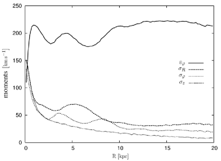
Figure 2: Dependences of $\bar{v}_{\varphi}$, $\sigma_{R}$, $\sigma_{\varphi}$, and $\sigma_{z}$ on $R$ in the FSLC.O model constructed by the Orbit.NB method.

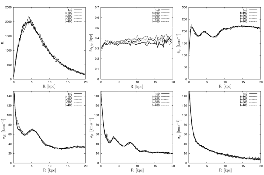
Figure 3: Initial evolutionary stages for the FSLC.O model. The upper snapshots show the disc views face-on for various moments of time (0, 100, 200, 300 and 400 Myr); the grey intensities correspond to the logarithms of particle numbers in the pixels. Middle and bottom panels show the dependences of various disc parameters on the cylindrical radius $R$ for various moments of time. Here $n$ is the number of particles in concentric cylindrical layers; $2z_{1/2}$ is twice the median of the value $|z|$ (it is a parameter of the disc thickness, see Sotnikova & Rodionov 2006); $\bar{v}_{\varphi}$, $\sigma_{R}$, $\sigma_{\varphi}$, $\sigma_{z}$ are four moments of the velocity distribution.

An interesting question arises in connection with the FSLC.O model equilibrium: how do the moments of the velocity distribution satisfy the equilibrium Jeans equations (see Binney & Tremaine 1987):

$$\left\{\begin{array}[]{rcl}{\overline{v}}_{\varphi}^{2}&=&v_{\rm c}^{2}+\sigma_{R}^{2}-\sigma_{\varphi}^{2}+\displaystyle\frac{R}{\rho_{\rm disk}}\frac{\partial(\rho_{\rm disk}\sigma_{R}^{2})}{\partial R}\,,\\ \sigma_{\varphi}^{2}&=&\displaystyle\frac{\sigma_{R}^{2}R}{2\overline{v}_{\varphi}}\left(\frac{\partial\overline{v}_{\varphi}}{\partial R}+\frac{\overline{v}_{\varphi}}{R}\right)\,,\\ \displaystyle\frac{\partial(\rho_{\rm disk}\sigma_{z}^{2})}{\partial z}&=&-\rho_{\rm disk}\displaystyle\frac{\partial\Phi_{\rm tot}}{\partial z}\,.\\ \end{array}\right.$$ (9)

Here $\Phi_{\rm tot}=\Phi_{\rm disk}+\Phi_{\rm ext}$. Fig. 4 shows the radial profiles of $\bar{v}_{\varphi}$, $\sigma_{\varphi}$, and $\sigma_{z}$ from the FSLC.O model and from the Jeans equations (9) (see also RS06). It can be seen that the model follows the Jeans equations very well. This is an unexpected finding, especially considering such unusual moment profiles.

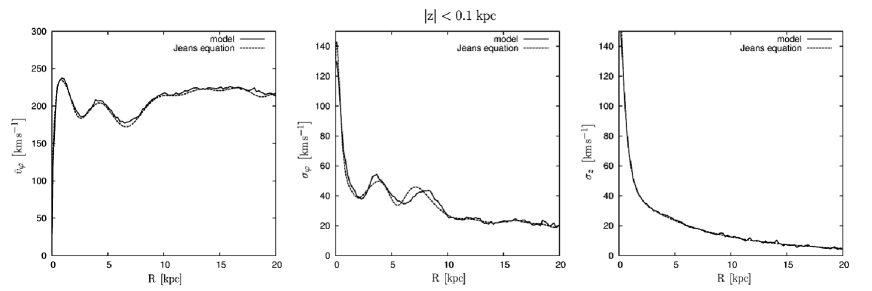
Figure 4: Comparison of profiles of the velocity distribution moments calculated from the Jeans equations and from the FSLC.O model. All moments for the disc were calculated inside the region $|z|<0.1\;{\rm kpc}$. Left panel: the solid line corresponds to the value $\bar{v}_{\varphi}$ for the model, and the dashed line corresponds to the same value calculated from the Jeans equation (the first equation of the system (9)), where the values $\sigma_{R}$ and $\sigma_{\varphi}$ were taken from the model. Middle panel: the solid line corresponds to the value $\sigma_{\varphi}$ for the model, and the dashed line corresponds to the same value calculated from the Jeans equation (the second equation of the system (9)), where the values $\bar{v}_{\varphi}$ and $\sigma_{R}$ were taken from the model. Right panel: the solid line corresponds to the value $\sigma_{z}$ for the model, and the dashed line corresponds to the same value calculated from the Jeans equation (the third equation of the system (9)).

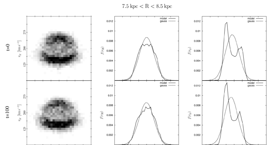
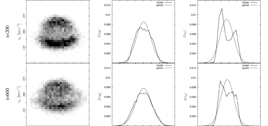
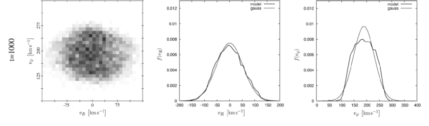
Figure 5: The velocity distributions for the FSLC.O model at various moments of time (0, 100, 200, 600, and 1000 Myr). The region of the disc within the range $7.5\,{\rm kpc}<R<8.5\,{\rm kpc}$ is considered. Left column: two-dimensional velocity distribution (the abscissa is the radial velocity $v_{R}$ and the ordinate is the azimuthal velocity $v_{\varphi}$); the grey intensities correspond to the numbers of particles that have velocities in the corresponding pixels. Middle column: one-dimensional distribution of the velocity $v_{R}$. Right column: one-dimensional distribution of the velocity $v_{\varphi}$. In the middle and right columns, the solid lines show the model distributions, and the dashed lines correspond to the Gaussians with parameters (mean and dispersion) taken from the models.

Another important feature of the FSLC.O model is that the velocity distribution in this model is far from the Schwarzschild distribution. The velocity distributions in the solar neighbourhood (near $R=8\;\rm kpc$) are shown in Fig. 5. Initially, both radial and azimuthal velocity distributions are far from Gaussian, although such unusual distributions are more or less in equilibrium. At least, they are conserved during the initial stages of evolution. However, these distributions are unstable, and they change substantially after about 500 Myr. After about 1 Gyr, the distributions are smoothed and tend to Gaussians.

Above we have discussed the self-consistent evolution of the FSLC.O model. It is also interesting, however, to examine a non-self-consistent evolution of this model; that is, to calculate the evolution of $N$ test particles in the total potential of the FSLC model. As expected, the model practically does not change during such “evolution” (at least on a time-scale of 10 Gyr). In particular, the density profile and non-Schwarzschild velocity distribution do not change. Thus, this shows again that this non-Schwarzschid velocity distribution is in equilibrium.

All models constructed using the Orbit.NB approach have the following properties. They are close to equilibrium. Moreover, the velocity distributions in the models are non-Schwarzschild ones and may have various forms. However, the velocity distributions tend to the Schwarzschild distribution during the dynamical evolution on a time-scale of 1 Gyr. Thus, although these models are close to equilibrium, they are probably non-physical because of their non-Schwarzschild velocity distributions. The arguments are as follows.

• The velocity distribution of the stars in the solar neighbourhood is similar to the Schwarzschild distribution (see, for example, Binney & Merrifield 1998).

• The constructed non-Schwarzschild velocity distributions are almost in equilibrium, but are unstable. The velocity distributions always tend to the Schwarzschild one during the evolution.

• In the models constructed using the Nbody.NB approach, the final velocity distributions are close to the Schwarzschild distribution (see Fig. 6). We note that the Nbody.NB and Orbit.NB approaches differ only in the method of evolution simulations in the iterations (see Section 3.2.3).

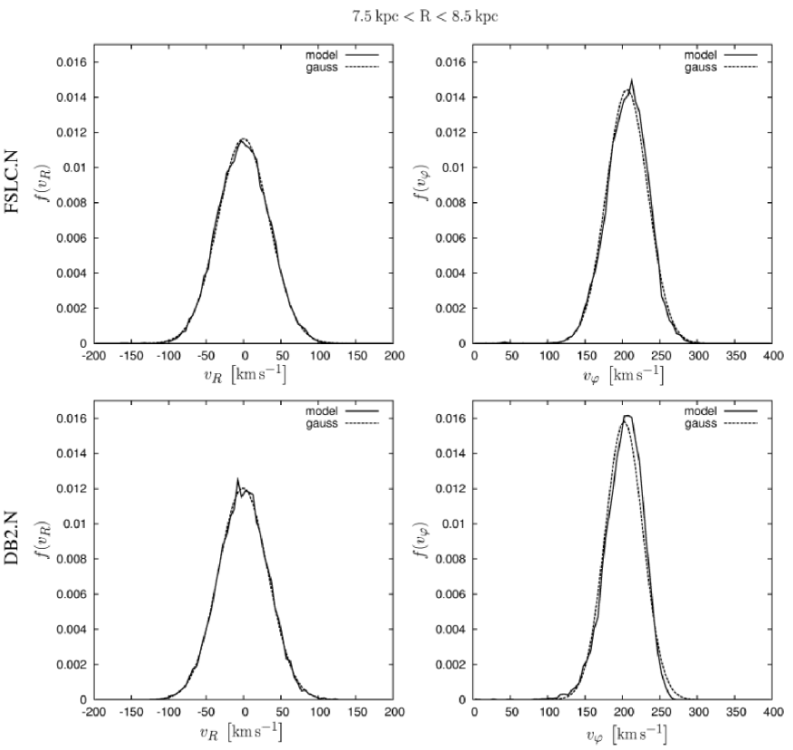
Figure 6: The distributions of radial and azimuthal velocities in the solar neighbourhood in the models constructed using the Nbody.NB approach. We consider the disc region of $7.5\;{\rm kpc}<R<8.5\;{\rm kpc}$. Left panels: the distributions of radial velocities. Right panels: the distributions of azimuthal velocities. The upper pictures were constructed for the FSLC.N model, and the lower ones for the DB2.N model. Description of both models is given in Section 5.2. The solid lines show the model distributions, and the dashed lines correspond to the Gaussians with parameters (mean and dispersion) taken from the models.

Generally speaking, we can assume that such unusual non-Schwarzschild velocity distributions will survive only in the “hothouse” conditions of the Orbit.NB approach because the evolution simulation in this approach is carried out non-self-consistently (see Section 3.2.3). When the conditions are close to realistic (as in the Nbody.NB approach), such distributions are smoothed and gradually converge to the Schwarzschild distribution.

4.2 Uniqueness hypothesis

In RS06, the authors formulated a hypothesis of uniqueness: not more than one equilibrium model (one equilibrium distribution function) can exist for a fixed density $\rho_{\rm disk}(R,z)$ and potential $\Phi_{\rm ext}(R,z)$ and a fixed kinetic energy fraction of residual motions (e.g. a fixed angular momentum $L_{z}$).

We can now say that in such a form the hypothesis is false. We can construct using the Orbit.NB approach as many equilibrium models as we want for the same $\rho_{\rm disk}(R,z)$, $\Phi_{\rm ext}(R,z)$ and fixed $L_{z}$. However, although these models are close to equilibrium, they probably bear no relation to actual stellar systems.

At the same time, the models constructed by the Nbody.NB approach are the same (within the noise level) for arbitrary initial states at the same $\rho_{\rm disk}(R,z)$, $\Phi_{\rm ext}(R,z)$ and fixed $L_{z}$. Moreover, the velocity distributions in constructed models are always close to the Schwarzschild distribution. Based on this fact and the probable non-physical character of the Orbit.NB models, one can formulate a hypothesis that the “physical” discs in the equilibrium state are unique. This hypothesis could be formulated as follows. When the functions $\rho_{\rm disk}(R,z)$ and $\Phi_{\rm ext}(R,z)$ are fixed and a fraction of the kinetic energy in the residual motions is also fixed (e.g. the value of the angular momentum $L_{z}$ is fixed), not more than one physical model in the equilibrium state may exist (the physical model is the model that can exist in reality). We think that the main feature of a real stellar disc is an almost Schwarzschild velocity distribution.

Whether or not our hypothesis is true is very important. If we know the mass distribution in the Galaxy and our hypothesis is valid, we can use our Nbody.NB method to reconstruct the velocity distribution in the Galactic disc. In other words, we can construct a phase model of the Galactic disc, and this model will correspond exactly to the real Galactic disc.

5 Phase models of the galactic stellar disk

5.1 Choice of model among the family of models

For the construction of phase models of the Milky Way Galactic disc, we use the Nbody.NB approach (see Section 3.2). Using this method, one can construct a family of models for the fixed functions $\rho_{\rm disk}(R,z)$ and $\Phi_{\rm ext}(R,z)$. This is a one-parameter family, and the parameter is the fraction of kinetic energy of residual motions (in other words, the disc “heat” degree). In our approach, this parameter is the value of $L_{z}$. We emphasize that, using the Nbody.NB approach, when we fix the value of $L_{z}$ we obtain the same model (within the noise level) regardless of the initial state.

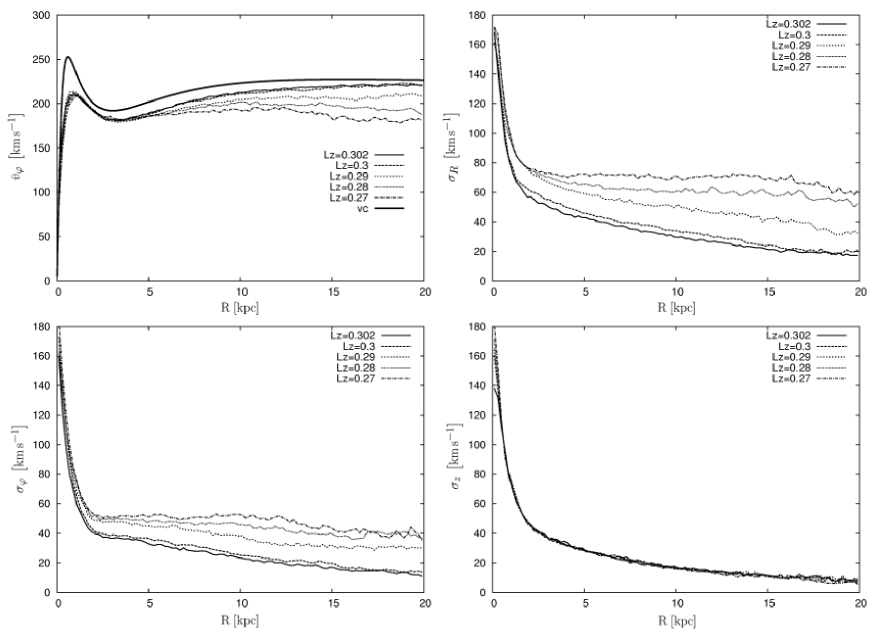
Figure 7: The family of phase models constructed using the Nbody.NB approach for the FSLC density model. For each model, we show the dependences of $\bar{v}_{\varphi}$, $\sigma_{R}$, $\sigma_{\varphi}$, and $\sigma_{z}$ on $R$. The moments were calculated in cylindrical layers infinite along the $z$-axis. In the upper left panel, the circular velocity curve is shown by the thick solid line. Models constructed for $L_{z}=0.302,\,0.3,\,0.29,\,0.28,\,0.27$ are represented. The model with $L_{z}=0.302$ is the FSLC.N model corresponding to the Galactic stellar disc.

A family of the $N$-body models for the FSLC density model is shown in Fig. 7 as an example. The parameters of the models are given below. One can ask how we choose the best-fitting model among the family. We have comparatively reliable kinematic Galactic parameters in the solar neighbourhood (see, for example, Binney & Merrifield 1998; Dehnen & Binney 1998b), so it is reasonable to use them to choose the model. One needs to choose any one parameter that on the one hand is well known in the solar neighbourhood, and on the other depends strongly on the disc “heat”. In other words, this value has to be strongly dependent on the value of $L_{z}$. For example, the velocity ellipsoid parameters $\bar{v}_{\varphi}$, $\sigma_{R}$, $\sigma_{\varphi}$, and $\sigma_{z}$ are well known. The value $\sigma_{z}$ is not suitable, because it does not depend on $L_{z}$ (see Fig. 7 and RS06). The value $\bar{v}_{\varphi}$ is also unsuitable, because it depends weakly on $L_{z}$ for cold models (see Fig. 7). The choice between the two values $\sigma_{R}$ and $\sigma_{\varphi}$ is somewhat arbitrary. We prefer the value $\sigma_{R}$ for the model choice.

There are various estimates of the value of $\sigma_{R}$ in the literature. We have chosen the value $\sigma_{R}=35\;{\rm km}\,{\rm s}^{-1}$ that was estimated using an extrapolation to the zero heliocentric distance (see Orlov et al. 2006). In addition, we adopted the solar distance from the Galactic centre as $R_{0}=8\;{\rm kpc}$ (see, for example, Nikiforov 2004; Avedisova 2005).

As a result, we have chosen the model in which the radial velocity dispersion in the solar neighbourhood is about $35\;{\rm km}\,{\rm s}^{-1}$. As the solar neighbourhood, we have chosen the region $7.9\;{\rm kpc}<R<8.1\;{\rm kpc}$ and $|z|<0.1\;{\rm kpc}$.

5.2 Models FSLC.N and DB2.N

We have considered two families of stellar disc models constructed for two Galactic density models (FSLC and DB2). The families of phase models were constructed using the Nbody.NB approach. From every family, we have chosen the stellar disc model that corresponds to the Galactic disc in the solar neighbourhood (in terms of the radial velocity dispersion). Hereafter we refer to these models as FSLC.N and DB2.N.

The family of models for the FSLC density model is shown in Fig. 7. It was constructed in the following way. We took as $\rho_{\rm disk}$ the disc density distribution from the FSLC model, and as $\Phi_{\rm ext}$ the potential arising from all FSLC model components except the disc. The disc density was taken as equal to zero at $R>R_{\rm max}=30\;{\rm kpc}$ or $|z|>z_{\rm max}=10\;{\rm kpc}$. We considered an initial cold model in which the particle orbits are circular. Four iteration sets with increasing accuracies were calculated. The parameters of the sets are shown in Table 3. The number of neighbours in the velocity distribution transfer is $n_{\rm nb}=10$. The time of one iteration is $t_{i}=50\;{\rm Myr}$. The FSLC.N model was constructed for the angular momentum $L_{z}=0.302$ (this value is given in our system of units as described in Section 4.1).

Table 3: The parameters of four iteration sets for the family of models constructed using the Nbody.NB approach for the FSLC and DB2 density models. Here, $n_{\rm it}$ is the number of iterations, $N$ is the number of bodies, $dt$ is the integration step, $\epsilon_{f}$ is the softening length for the FSLC model, and $\epsilon_{d}$ is the softening length for the DB2 model. The softening length was chosen using the recommendations of Rodionov & Sotnikova (2005).

$n_{\rm it}$	N	$dt,\;{\rm Myr}$	$\epsilon_{f},\;{\rm kpc}$	$\epsilon_{d},\;{\rm kpc}$
500	20,000	1	0.04	0.04
200	100,000	0.5	0.02	0.02
100	500,000	0.5	0.02	0.01
5	500,000	0.05	0.02	0.01

The family of models for the DB2 density model, in particular the DB2.N model, was constructed in the following way. The density of the thin stellar disc in the DB2 model was taken as $\rho_{\rm disk}$, and the potential arising from all components except the thin stellar disc was taken as $\Phi_{\rm ext}$. The disc density at $R>R_{\rm max}=30\;{\rm kpc}$ or $|z|>z_{\rm max}=10\;{\rm kpc}$ was taken as equal to zero. This is the same condition as in the FSLC model. Here we again consider the cold initial model with circular orbits. Four sets of iterations were again calculated. The parameters of these sets are shown in Table 3. We have adopted the parameters $n_{\rm nb}=10$, $t_{i}=50\;{\rm Myr}$. The DB2.N model was constructed for the angular momentum $L_{z}=0.1595$ (this value is given in our system of units as described in Section 4.1).

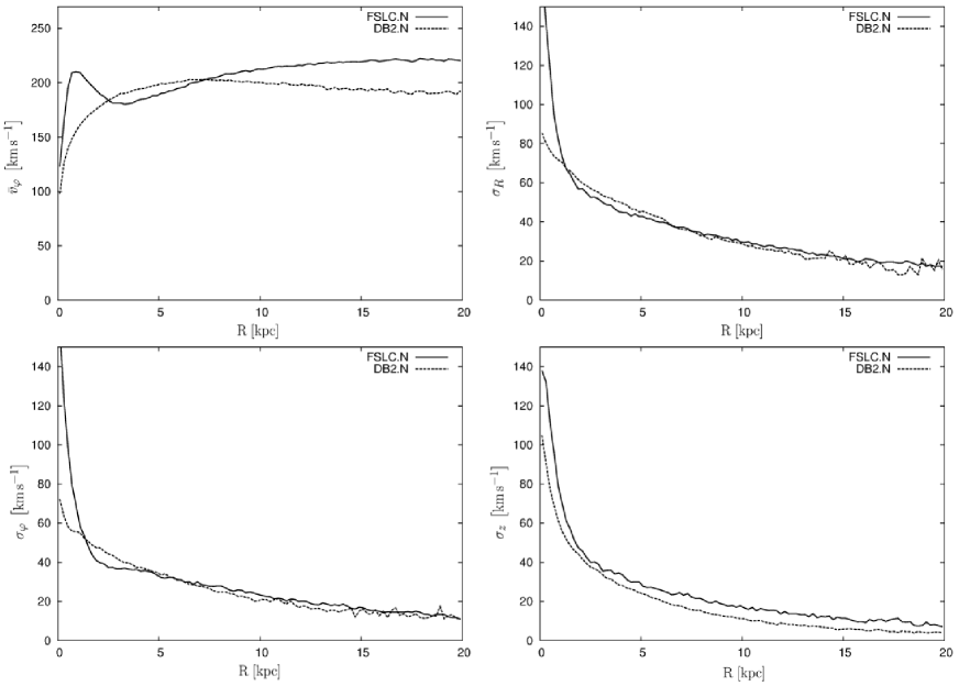
Figure 8: The dependences of four velocity distribution moments $\bar{v}_{\varphi}$, $\sigma_{R}$, $\sigma_{\varphi}$, and $\sigma_{z}$ on the cylindrical radius $R$ for the FSLC.N and DB2.N models. The moments were calculated in cylindrical layers infinite along the $z$-axis.

The radial profiles of the velocity distribution moments for the FSLC.N and DB2.N models are shown in Fig. 8. Let us consider the profiles of $\sigma_{R}$ and $\sigma_{\varphi}$. In the central parts of the models, these profiles are very different. This is caused by the more massive and concentrated bulge in the FSLC.N model with respect to the DB2.N model (see Fig. 1 in Section 2). However, the profiles of $\sigma_{R}$ and $\sigma_{\varphi}$ for the two models are similar from about $2-3$ kpc. This is in spite of the difference between the initial density models. In particular, one can observe a different relative disc contribution in the total mass and rotation curve (see Fig. 1). Fig. 8 also shows that the profiles of $\sigma_{z}$ are different. However, we note that the value of $\sigma_{z}$ at any point is defined only by the density distribution. This fact is a consequence of the last Jeans equation (9). Our phase models satisfy the Jeans equations very well, however, and therefore the differences in the $\sigma_{z}$ profiles are explained by the differences in the density models.

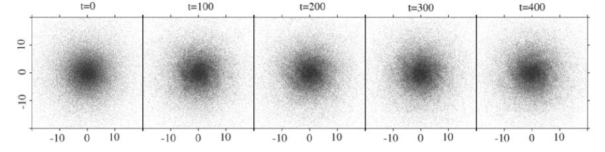
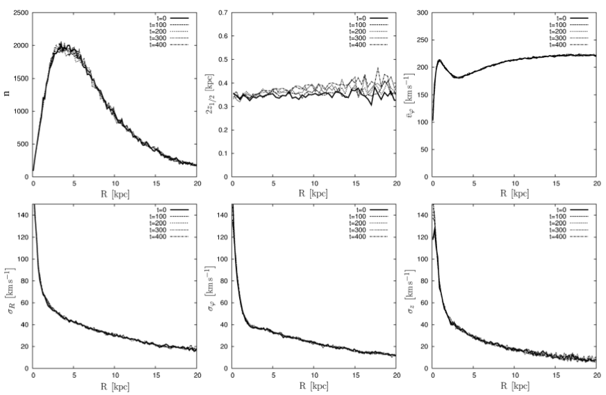
Figure 9: Initial evolution stages of the FSLC.N model. The same values are shown as in Fig. 3. The evolution simulation used the following parameters: number of bodies $N=100\,000$, integration step $dt=0.04\;\rm Myr$, softening length $\epsilon=0.025\;\rm kpc$. The two last parameters were chosen according to the recommendations of Rodionov & Sotnikova (2005).

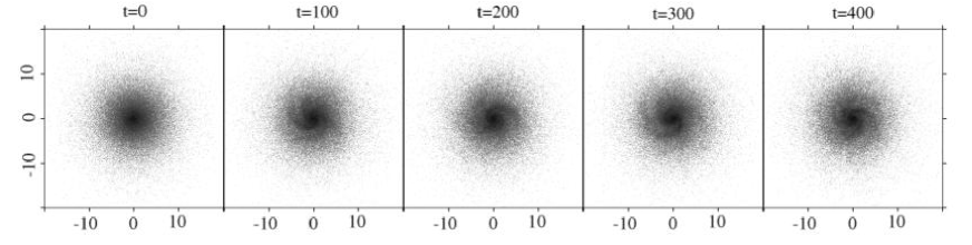
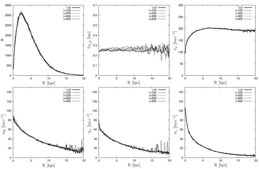
Figure 10: Initial evolution stages of the DB2.N model. The same values are shown as in Fig. 3. The evolution simulation used the following parameters: number of bodies $N=100\,000$, integration step $dt=0.04\;\rm Myr$, softening length $\epsilon=0.015\;\rm kpc$. The two last parameters were chosen according to the recommendations of Rodionov & Sotnikova (2005).

The initial stages of the evolution for the FSLC.N and DB2.N models are shown in Figs 9 and 10. Both models conserve the structural and dynamical parameters in the early stages of the evolution very well. Therefore both models are close to equilibrium.

6 Conclusions

In this paper, we have discussed the problem of constructing a phase model of the Galactic stellar disc. We used the iterative method proposed in RS06. The realization of the iterative method described in RS06 (Nbody.SCH approach) has some disadvantages. The Nbody.SCH method has a problem with the construction of a relatively cold stellar disc. Furthermore, the Nbody.SCH method cannot be directly applied to stellar systems with arbitrary geometry. The main goal of this study was to develop a new realization of the iterative method without the disadvantages of the Nbody.SCH approach. For this purpose, we considered a number of modifications of the iterative method (Nbody.SCH, Orbit.SCH, Nbody.NB, and Orbit.NB). The Nbody.NB method satisfied our conditions. This method can be directly applied for the construction of phase models of stellar systems with arbitrary geometry. The method is simple in terms both of understanding and of implementation. Using the Nbody.NB approach, we have constructed phase models of the Galactic disc for two realistic density models (suggested by Flynn, Sommer-Larsen & Christensen 1996; Dehnen & Binney 1998a).

For a given mass distribution model of the Galaxy, we can construct a one-parameter family of equilibrium models of the Galactic disc. From this family we can choose a unique model using local kinematic parameters that are known from the Hipparcos data. There are, however, two important questions. Is there an equilibrium disc model besides the models from this one-parameter family? Does the real Galactic disc belong to this one-parameter family? (Of course this family should be constructed for a real mass model of the Galaxy.) The answer to the first question is affirmative. Using the Orbit.NB method, we can construct many models besides the models from this one-parameter family. We have, however, shown that these models are probably non-physical. Based on this fact, we suppose that all models except models from this one-parameter family are non-physical. Consequently, we think that the answer to the second question is also affirmative. However, we cannot strictly prove it as yet. We think that the key to the proof is Schwarzschild velocity distributions. The models from our one-parameter family have almost such velocity distributions, and we think that the velocity distributions in real galactic discs are close to the Schwarzschild distribution.

We now discuss possible applications of our Nbody.NB method.

This method can be used to construct phase models of stellar systems with arbitrary geometry. For example, the method can be used to construct phase models of triaxial elliptical galaxies.

Here we have used the iterative method to construct a phase model of the stellar disc of a spiral galaxy. In the future, we are going to construct a self-consistent model of a spiral galaxy (including live halo and bulge) using a modified Nbody.NB approach.

Another, rather more important, direction of future investigations is a comparison of our iterative models with observations of real galaxies. This comparison will make it possible to derive from observations the constraints on unobservable parameters of galaxies (for example dark matter mass and its profile). Of course, such a comparison should first be carried out for the Milky Way. One of the possible schemes is as follows. If we know the mass distribution in the Galaxy then using our method we can construct a phase model of the Galactic disc. The mass distribution in the Galaxy contains two parts — visible and dark matter. From the phase model of the Galactic disc, we can derive the profiles of stellar kinematic parameters (profiles of velocity dispersions and mean azimuthal velocity). Let us assume that we know from observations the mass distribution of visible matter and the profiles of stellar kinematic parameters. Then, using the iterative method, we can put some constraints on the dark matter mass distribution. The distribution of the dark matter should be such that the iterative model has the observable kinematics. At the moment, observational profiles of stellar kinematic parameters have fairly large uncertainties; however, it is expected that the GAIA mission will provide a much higher accuracy for these data. We are planning to study which constraints on the Milky Way parameters we can obtain from GAIA using our iterative models.

The iterative method can also be used to derive the velocity dispersion profiles from observations. It is impossible to obtain the velocity dispersion profiles for external spiral galaxies directly from observations, which can yield only the line-of-sight velocity, $v_{\rm los}$, and the line-of-sight velocity dispersion, $\sigma_{\rm los}$. However, we can use the Jeans equations to derive the velocity dispersion profiles from the observed quantities $v_{\rm los}$ and $\sigma_{\rm los}$. In practice, however, one has to include some a priori assumptions about the form of the velocity dispersion profiles. In the literature, authors have made slightly different assumptions, but all of them are based on the hypothesis that the velocity dispersion in the radial direction is proportional to the velocity dispersion in the vertical direction (see section 3 in RS06).

Using our iterative method, we can derive the velocity dispersion profiles from line-of-sight parameters without any additional assumptions. The general idea is as follows. From observations we have (more or less precisely) the distribution of visible mass and some constraints on the distribution of dark matter. If we fix the mass distribution in a galaxy (for visible and dark matter) then, using the iterative method, we can construct a one-parameter family of phase models of the galactic disc. The parameter of this family is the degree of disc heating (for example the fraction of the kinetic energy of the disc contained in residual motions). Using observable profiles of $v_{\rm los}$ and $\sigma_{\rm los}$, we can choose a unique model from this family. As a result, we will have a phase model of the galactic disc. From this model we can calculate the velocity dispersion profiles.

References

- Avedisova (2005) Avedisova V.S., 2005, Astron. Rep., 49, 435
- Barnes & Hut (1986) Barnes J., Hut P., 1986, Nature, 324, 446
- Binney & Merrifield (1998) Binney J., Merrifield M., 1998, Galactic Astronomy. Princeton Univ. Press, Princeton
- Binney & Tremaine (1987) Binney J., Tremaine S., 1987, Galactic Dynamics. Princeton Univ. Press, Princeton
- Dehnen & Binney (1998a) Dehnen W., Binney J., 1998a, MNRAS, 294, 429
- Dehnen & Binney (1998b) Dehnen W., Binney J., 1998b, MNRAS, 298, 387