A Statistical Method for Estimating Luminosity
Functions using Truncated Data

Abstract

The observational limitations of astronomical surveys lead to significant statistical inference challenges. One such challenge is the estimation of luminosity functions given redshift $(z)$ and absolute magnitude $(M)$ measurements from an irregularly truncated sample of objects. This is a bivariate density estimation problem; we develop here a statistically rigorous method which (1) does not assume a strict parametric form for the bivariate density; (2) does not assume independence between redshift and absolute magnitude (and hence allows evolution of the luminosity function with redshift); (3) does not require dividing the data into arbitrary bins; and (4) naturally incorporates a varying selection function. We accomplish this by decomposing the bivariate density $\phi(z,M)$ via

$$\log\phi\!\left(z,M\right)={\bf f}\!\left(z\right)+{\bf g}\!\left(M\right)+{\bf h}\!\left(z,M,\theta\right)$$

where ${\bf f}$ and ${\bf g}$ are estimated nonparametrically, and ${\bf h}$ takes an assumed parametric form. There is a simple way of estimating the integrated mean squared error of the estimator; smoothing parameters are selected to minimize this quantity. Results are presented from the analysis of a sample of quasars.

1 Introduction

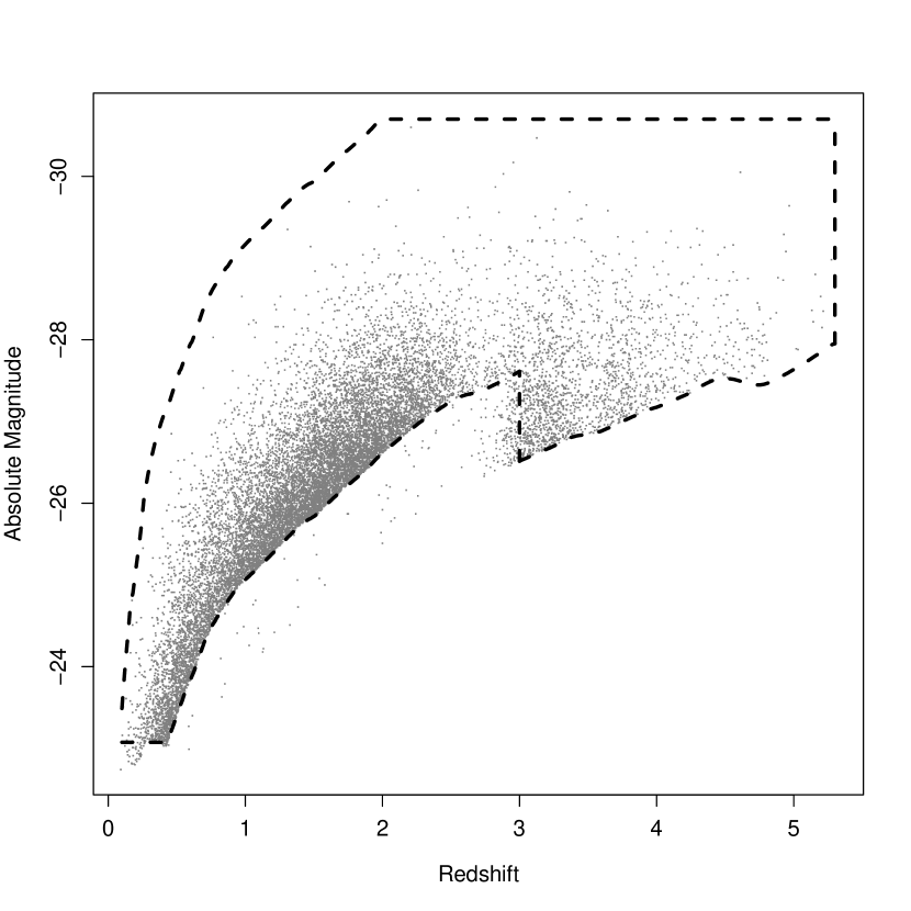
Figure 1: Quasar data from the Sloan Digital Sky Survey, the sample from Richards et al. (2006). Quasars within the dashed region are used in this analysis. The removed quasars are those with $M\leq-23.075$, which fall into the irregularly-shaped corner at the lower left of the plot, and those with $z\leq 3$ and apparent magnitude greater than 19.1, which fall into a very sparsely sampled region.

Astronomers commonly seek to estimate the space density of objects, and a sky survey such as the Sloan Digital Sky Survey (SDSS) (York et al., 2000) can yield a representative sample useful for this purpose, due to the assumed isotropy of the Universe. Figure 1 depicts redshift and absolute magnitude measurements for a sample of quasars given in Richards et al. (2006). These are a subset of the SDSS quasar sample (Data Release 3), chosen to be statistically valid for purposes such as exploring the evolution with redshift of the luminosity function, i.e. the space density of quasars as a function of absolute magnitude. This paper describes a new method for estimating these luminosity functions, and presents results from the analysis of this quasar sample.

For the purposes of the statistical inference problem, imagine the dots in Figure 1 as observations of bivariate data $\{(z_{i},M_{i})\!:i=1,2,\ldots,n\}$ from some distribution with probability density $\phi(z,M)$, i.e. the probability that a randomly chosen quasar falls in a region $B$ is $\int_{B}\phi(z,M)dz\>dM$. (Equivalently, in a sample of size $n$, one expects that $n\int_{B}\phi(z,M)dz\>dM$ will fall in the region $B$.) Hence, the luminosity function at redshift $z$ is, up to a multiplicative constant, the cross-section of the bivariate density at $z$, denoted $\phi(z,*)$.

The main challenge is estimation of this bivariate density given truncated data. Only objects with apparent magnitude within some range are observable. When this bound on apparent magnitude is transformed into a bound on absolute magnitude, the truncation bound takes an irregular shape, varying with redshift. $K$-corrections further complicate this boundary, leading to the dashed region in Figure 1. Also, the sample is not assumed to be complete within this region, and the probability of observing an object will vary with position on the sky, along with other factors. Incorporating this selection function into the analysis is a secondary challenge.

Nonparametric estimators are advantageous in cases where either there does not exist a commonly agreed upon parametric physical model, or there is a desire to validate a parametric model. See Wasserman et al. (2001) for an overview of the potential of nonparametric methods in astronomy and cosmology. A fully nonparametric approach is not possible here, since some assumptions must be placed on the form of the density in order to infer its shape over the unobservable region. Under such conditions, one approach would be to fit a sequence of increasingly complex parametric models in an attempt to obtain a good fit to the data. A less subjective alternative is a semiparametric approach which merges a nonparametric method with sufficient structure from a parametric form to obtain useful results. This work describes a semiparametric approach to estimating the bivariate density, and hence the luminosity functions, under irregular truncation.

This is a long-standing challenge in astronomical data analysis, with a variety of proposed methods. Interesting qualitative and simulations-based comparisons between different approaches can be found in Willmer (1997) and Takeuchi et al. (2000). A parametric model fit using maximum likelihood is a common choice, since it addresses the truncation bias in a natural manner; see, for instance, Sandage et al. (1979), Boyle et al. (2000) and the parametric models fit and referenced in §6 of Richards et al. (2006). These models have the drawback of imposing a tight constraint on the luminosity function in a case where there is not a consensus parametric form.

Some proposed methods are nonparametric, but assume that redshift and absolute magnitude are independent, and hence assume that there is no evolution of the luminosity function with redshift. These include the nonparametric maximum likelihood method described in Lynden-Bell (1971) and Jackson (1974) and adapted for double truncation in Efron & Petrosian (1999), along with the methods in Efstathiou (1988), Choloniewski (1986), the $1/V_{\rm max}$ estimator of Schmidt (1968) and Felten (1976). The semiparametric method of Wang (1989) also assumes independence. Maloney & Petrosian (1999) apply a nonparametric technique which assumes independence after having transformed the bivariate data using a parametric form. Any method which assumes independence can be applied over small redshift ranges (usually called bins). Nicoll & Segal (1983) and Page & Carrera (2000) describe other binning approaches. Binning forces the difficult choices of bin centers and widths, and independence is still assumed over the width of the bin.

This work was motivated by the goal of developing a statistically rigorous method which (1) does not assume a strict parametric form for the bivariate density; (2) does not assume independence between redshift and absolute magnitude; (3) does not require dividing the data into arbitrary bins; and (4) naturally incorporates a varying selection function. This was accomplished by decomposing the bivariate density $\phi(z,M)$ into

$$\log\phi\!\left(z,M\right)={\bf f}\!\left(z\right)+{\bf g}\!\left(M\right)+{\bf h}\!\left(z,M,\theta\right)$$ (1)

where ${\bf h}(z,M,\theta)$ will take an assumed parametric form; it is intended to model the dependence between the two random variables. For example, there may be a physical, parametric model for the evolution of the luminosity function which could be incorporated into ${\bf h}(z,M,\theta)$. Alternatively, one could use ${\bf h}(z,M,\theta)=\theta zM$ as a first-order approximation to the dependence. The functions ${\bf f}$ and ${\bf g}$ are estimated nonparametrically, with bandwidth parameters to control the amount of smoothness in the estimate. Using the quasar sample of Figure 1, the estimates obtained here are quite consistent, if not a bit smoother, than those found in Richards et al. (2006). This analysis confirms the finding of the flattening of the slope of the luminosity function at higher redshift.

The paper is organized as follows. §2 briefly describes the quasar sample used here. §3 gives an overview of the idea of local maximum likelihood, a nonparametric extension of maximum likelihood, and describes in detail the semiparametric approach taken here. §4 describes how the integrated mean squared error can be approximated using cross-validation; the bandwidths can then be chosen to minimize this quantity. §5 presents some results from the analysis of the Richards et al. (2006) quasar sample, along with the results from some simulations. More detailed derivations, along with theory for approximating the distribution of the estimator, can be found in Schafer (2006). The approach was implemented as a Fortran subroutine with R wrapper.

2 Data

The full Richards et al. (2006) sample, shown in Figure 1, consists of 15,343 quasars. From these, any quasar is removed if it has $z\geq 5.3$, $z\leq 0.1$, $M\geq-23.075$, or $M\leq-30.7$. In addition, for quasars of redshift less than 3.0, only those with apparent magnitude between 15.0 and 19.1, inclusive, (after the application of $K$-corrections) are kept; for quasars of redshift greater than or equal to 3.0, only those with apparent magnitude between 15.0 and 20.2 are retained. These boundaries combine to create the irregular shape shown by the dashed line in Figure 1. This truncation removes two groups of quasars from the Richards et al. (2006) sample. First, there are 62 quasars removed with $M\geq-23.075$. This was done to mitigate the effect of the irregularly-shaped, very narrow region in the lower left corner of Figure 1. Second, there are 224 additional quasars with $z\leq 3$ and apparent magnitude larger than 19.1; these fall in an extremely poorly sampled region, which can also be noted from Figure 1. Hence there are 15,057 quasars remaining after this truncation.

The sample is not assumed to be complete within this region. Associated with each sampled quasar is a value for the selection function, which can be interpreted as the probability that a quasar at this location, and of these characteristics would be captured by the sample. Details regarding how the selection function was approximated via simulations, along with many other details regarding the sample, can be found in Richards et al. (2006).

3 The Model

The approach taken here is built upon a nonparametric extension of maximum likelihood called local likelihood modeling. This section begins by describing local likelihood density estimation in the general case. This is then adapted to the problem at hand, initially for the case assuming the random variables are independent. The case where dependence is allowed is then described as a simple extension.

3.1 Local Likelihood Density Estimation

To contrast the standard global approach to estimation with the local approach employed here, consider the following. Assume the data ${\bf X}=(X_{1},X_{2},\ldots,X_{n})$ are realizations (observations) of independent, identically distributed random variables from a distribution with density $f_{\mbox{\tiny 0}}$. With classic maximum likelihood estimation, one chooses a single estimate from among a class of candidates for $f_{\mbox{\tiny 0}}$; let ${\cal F}$ denote this class. Specifically, the maximum likelihood estimator ($\widehat{f}_{\mbox{\tiny MLE}}$) for $f_{\mbox{\tiny 0}}$ is defined as the $f\in{\cal F}$ which maximizes

$$\sum_{j=1}^{n}\log f\!\left(X_{j}\right)-\left[n\!\left(\!\int\!f\!\left(x\right)dx-1\right)\right]$$ (2)

or, equivalently, the $f\in{\cal F}$ which maximizes

$$\sum_{j=1}^{n}\log f\!\left(X_{j}\right)-n\!\int\!f\!\left(x\right)dx.$$ (3)

(The notation $X_{j}$ simultaneously indicates a random variable with unknown density $f_{\mbox{\tiny 0}}$, and the observed realization of that random variable.) Although written here like a density estimation problem, one could imagine the class ${\cal F}$ being indexed by a parameter $\theta$; hence this also captures the usual maximum likelihood estimator for parametric problems. For example, one could define ${\cal F}$ to consist of all Gaussian densities as mean $\mu$ and variance $\sigma^{2}$ vary. In cases where each $f\in{\cal F}$ is a density (e.g., the aforementioned Gaussian case), the expression in brackets of equation (2) is always zero, and thus unnecessary. However, it is often advantageous to let ${\cal F}$ be a wider class of smooth, nonnegative functions; then the bracketed term forces $\widehat{f}_{\mbox{\tiny MLE}}$ to be a probability density.

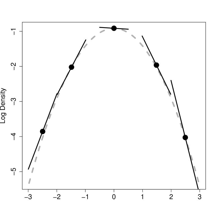
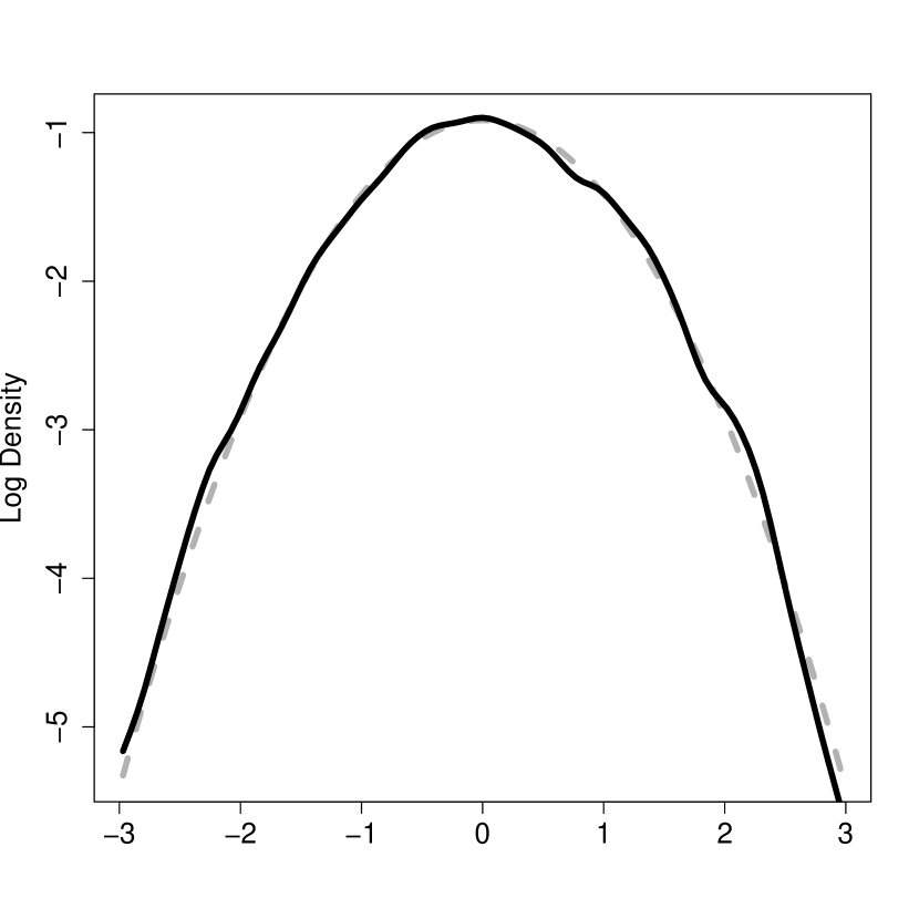
Figure 2: An illustration of local likelihood density estimation. The dashed line in both plots is the logarithm of the Gaussian density with mean zero and variance one ($f_{0}$ in the notation of §3.1). In the left plot, depicted are local linear estimates $(\widehat{f}_{u})$ of the density for each of $u\in\{-2.5,-1.5,0,1.5,2.5\}$. A simulated data set consisting of 10,000 values is utilized. In fact, local linear estimates are found for 101 values of $u$ equally spaced between -3 and 3. These local estimates are smoothed together to get the final estimate ($\widehat{f}_{\mbox{\tiny LL}}$) shown in the right plot.

With local modeling, instead of seeking the single member of the class ${\cal F}$ to be the estimate of $f_{0}$, the goal is to approximate $f_{0}(x)$ for $x$ near $u$, yielding the local estimate $\widehat{f}_{u}$. Typically, $\log f_{0}$ can be approximated locally by a polynomial; in fact, a linear form for $\log\widehat{f}_{u}$ usually suffices. See Figure 2. On the left plot, the dashed line gives the logarithm of the Gaussian density with mean zero and variance one. Local linear estimates $\log\widehat{f}_{u}$ are shown for each of $u\in\{-2.5,-1.5,0,1.5,2.5\}$. It is unimportant that $\widehat{f}_{u}(x)$ is not a good estimate of $f_{0}(x)$ for $x$ far from $u$, since many such local estimates will be found and then smoothed together. These local estimates were calculated with a simulated data set consisting of 10,000 values. The method for finding these local estimates is outlined next.

In independent work, Loader (1996) and Hjort & Jones (1996) localized the likelihood criterion of equation (3) near $u\in\hbox{I\kern-1.66702pt\hbox{R}}$ by writing

$${\cal L}_{u}\!\left(f_{u},{\bf X}\right)\equiv\sum_{j=1}^{n}K^{*}\left(X_{j},u,\lambda\right)\log f_{u}\!\left(X_{j}\right)-n\!\int\!\!K^{*}\left(x,u,\lambda\right)f_{u}\!\left(x\right)dx,$$ (4)

where $K^{*}\!(x,u,\lambda)$ is a kernel function parametrized by $\lambda>0$. A standard choice would be $K^{*}\!(x,u,\lambda)=K\!((x-u)/\lambda)$ where $K$ is a probability density, but more specific forms will be considered (and required) below. The choice of $\lambda$ typically has much more influence on the estimator than does the choice of the kernel function. The local estimate $\widehat{f}_{u}$ is found by maximizing ${\cal L}_{u}(f_{u},{\bf X})$ over $\log f_{u}$ belonging to some simple class, usually degree $p$ polynomials expanded around $u$:

$$\log f_{u}\!\left(x\right)=a_{u\mbox{\tiny 0}}+a_{u\mbox{\tiny 1}}\!\left(x-u\right)+\cdots+a_{up}\!\left(x-u\right)^{p}.$$ (5)

Thus, the model is locally parametric with parameters $a_{u\mbox{\tiny 0}},\ldots,a_{up}$. One imagines repeating this procedure at a grid of $u$-values, call this grid ${\cal G}$, and hence obtaining a family of local estimates $\widehat{\bf f}\equiv\{\widehat{f}_{u}\!:u\in{\cal G}\}$. As a result, $\widehat{\bf f}$ is the family ${\bf f}$ of local estimates which maximizes

$${\cal L}\!\left({\bf f},{\bf X}\right)\equiv\sum_{u\in{\cal G}}{\cal L}_{u}\!\left(f_{u},{\bf X}\right).$$ (6)

The final local likelihood estimator $\widehat{f}_{\mbox{\tiny LL}}$ is constructed by smoothing together the local estimates:

$$\widehat{f}_{\mbox{\tiny LL}}\!\left(x\right)\equiv\left(\sum_{u\in{\cal G}}K^{*}\left(x,u,\lambda\right)\widehat{f}_{u}\!\left(x\right)\right)\bigg{/}\left(\sum_{u\in{\cal G}}K^{*}\left(x,u,\lambda\right)\right),$$ (7)

thus making dual use of $\lambda$. Returning to Figure 2, the plot on the right shows $\widehat{f}_{\mbox{\tiny LL}}$, the result of smoothing together 101 local linear estimates (${\cal G}$ consists of 101 values between -3 and 3). In this case, $\lambda=0.05$. It is clear that the estimate comes very close to the true density.

In what follows, simply assume that $K^{*}$ is chosen so that

$$\sum_{u\in{\cal G}}K^{*}\left(x,u,\lambda\right)=1$$ (8)

for all $x$ and hence

$$\widehat{f}_{\mbox{\tiny LL}}\!\left(x\right)=\left(\sum_{u\in{\cal G}}K^{*}\left(x,u,\lambda\right)\widehat{f}_{u}\!\left(x\right)\right).$$ (9)

This is a departure from the original approach of Loader (1996) and Hjort & Jones (1996), who instead used $\widehat{f}(x)\equiv\widehat{f}_{x}(x)$.

The criterion ${\cal L}({\bf f},{\bf X})$ appears awkward upon first sight, but it possesses the following property: Considering $(X_{1},\ldots,X_{n})$ again as random variables with unknown density $f_{\mbox{\tiny 0}}$, then $\langle{\cal L}({\bf f},{\bf X})\rangle$ is maximized by choosing the family ${\bf f}$ which sets $f_{u}(x)=f_{\mbox{\tiny 0}}(x)$ for all $u$ and all $x$. If that choice were made, the estimate would be $\widehat{f}_{\mbox{\tiny LL}}=f_{\mbox{\tiny 0}}$. Thus, since ${\cal L}({\bf f},{\bf X})\approx\langle{\cal L}({\bf f},{\bf X})\rangle$, the local estimate $\log\widehat{f}_{u}$ will approximate the degree $p$ Taylor expansion of $\log f_{\mbox{\tiny 0}}(x)$ for $x$ around $u$. The expected value of the standard likelihood criterion is also maximized by setting the density equal to the truth, but this localized version has the advantage of allowing the choice of $\lambda$ to adjust the amount of smoothness in the estimator. In §4, an objective method for bandwidth selection is described. There is an apparent conflict between the choice of $\lambda$ and the choice of the number of local models (the cardinality of ${\cal G}$) since small ${\cal G}$ will lead to smooth estimates. In the applications here, ${\cal G}$ is chosen large, so that the amount of smoothing is completely dictated by $\lambda$.

3.2 Density Estimation under Truncation

Now return to the bivariate density estimation problem using truncated astronomical data. The available data are denoted ${\bf z}\equiv(z_{1},z_{2},\ldots,z_{n})$ and ${\bf M}\equiv(M_{1},M_{2},\ldots,M_{n})$, the vectors of redshifts and absolute magnitudes, respectively. Let ${\cal A}$ denote the region outside of which the data are truncated and let ${\cal A}(z,*)\equiv\{M\!:(z,M)\in{\cal A}\}$ denote the cross-section of ${\cal A}$ at $z$; ${\cal A}(*,M)$ is defined similarly. Let $\phi(z,M)$ denote the unknown joint density of random variables $z$ and $M$.

The approach taken here originates in the following naive method. For the moment assume $z$ and $M$ are independent so that $\phi(z,M)=f(z)g(M)$ where $f$ is the density for redshift and $g$ is the density for absolute magnitude. Clearly, the available data allow estimation of the redshift density for observable quasars, denote this density $f^{*}$. This is related to $f$ by

$$f^{*}\!\!\left(z\right)=k\!\int_{{\cal A}\left(z,*\right)}h\!\left(z,M\right)dM=kf\!\left(z\right)\!\int_{{\cal A}\left(z,*\right)}g\!\left(M\right)dM$$ (10)

where $k$ is a normalizing constant which forces $f^{*}$ to integrate to one. Assuming for the moment that $g$ were known, it is possible to turn an estimator for $f^{*}$ into an estimator for $f$ by solving equation (10) for $f$:

$$\widehat{f}_{\mbox{\tiny NAIVE}}\!\left(z\right)\propto\widehat{f}^{*}\!\left(z\right)\bigg{/}\left(\int_{{\cal A}\left(z,*\right)}g\!\left(M\right)dM\right).$$ (11)

Starting with an initial guess at $g$, we could iterate between assuming $g$ is known, and estimating $f$, and vice versa.

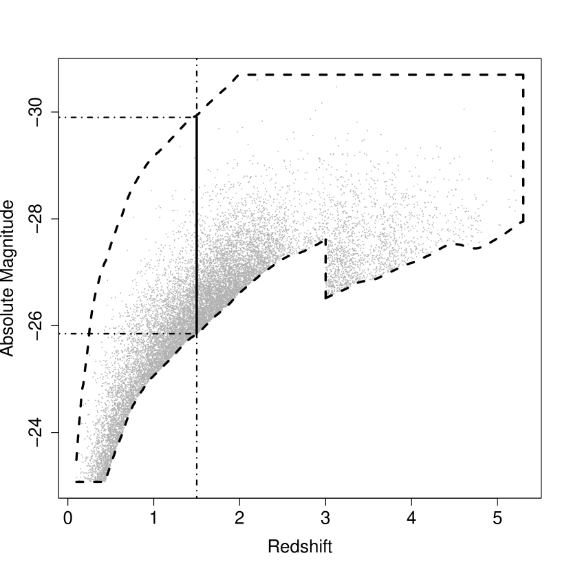
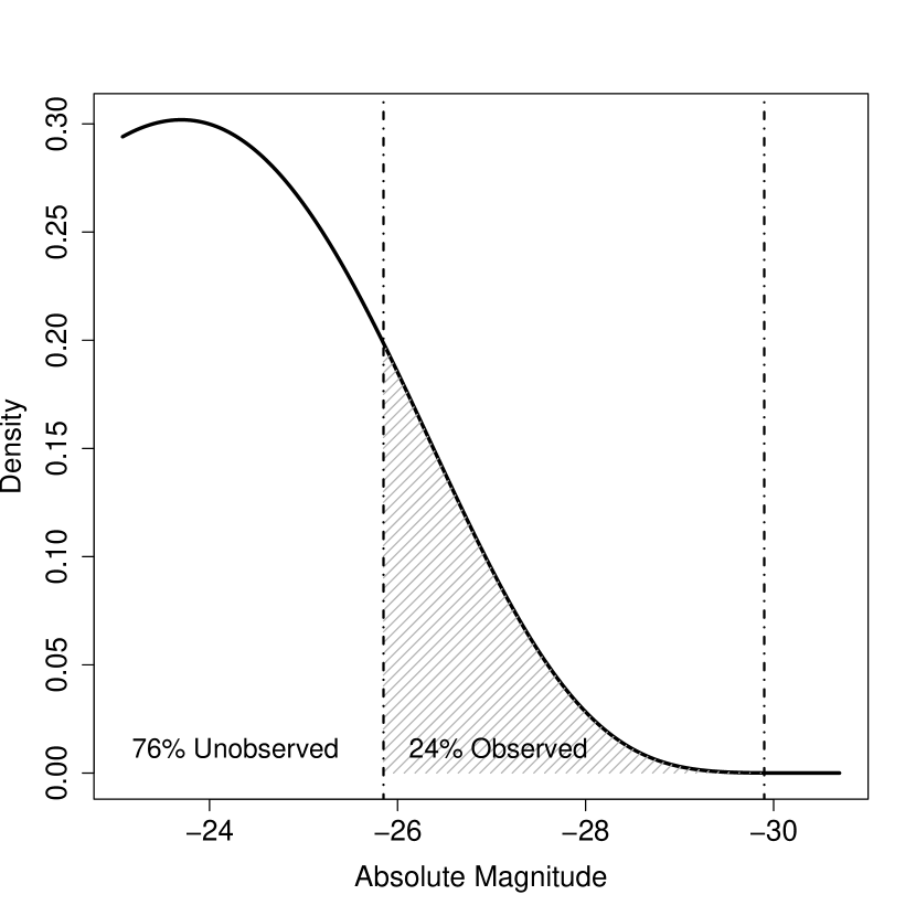
Figure 3: An explanation of the naive, but motivating idea. The left plot in the first row depicts the cross-section of the observable region at $z=1.5$ (denoted ${\cal A}(1.5,*)$) with absolute magnitudes ranging from -29.9 to -25.85. In the right plot, the solid curve is an assumed density for absolute magnitude. 24% of the area under this curve falls in ${\cal A}(1.5,*)$, thus one would assume that the observed sample catches 24% of the quasars at redshift $z=1.5$. (For now, ignore selection effects.) In the second row, the left plot shows how this proportion observed varies with redshift. The dashed line in the right plot is the estimated density for observable quasars ($\widehat{f}^{*}$), i.e. the estimate ignoring truncation. The solid curve is $\widehat{f}_{\mbox{\tiny NAIVE}}$, which equals $\widehat{f}^{*}$ divided by the curve on the left and then rescaling to make it a density. Note that the estimate at $z=1.5$ actually decreases after this adjustment because quasars are relatively well-observed at that redshift. Note how the sharp feature in the observable region at $z=3.0$ creates both the increase in proportion observed and the steep drop of $\widehat{f}_{\mbox{\tiny NAIVE}}$ at that redshift.

This procedure is portrayed in Figure 3. Using the quasar data set described in §2, the upper left plot depicts ${\cal A}(1.5,*)$ along the vertical axis, with absolute magnitudes ranging from -29.9 to -25.85. An (arbitrary) assumption is made regarding the density for absolute magnitude $(g)$, shown as the solid curve in the upper right plot. For example, one can find that

$$\int_{{\cal A}\left(1.5,*\right)}g\!\left(M\right)dM\approx 0.24,$$ (12)

and thus conclude that the observed sample catches 24% of the quasars at $z=1.5$. (The fact that some quasars are missed within ${\cal A}$ is considered later when the selection function is incorporated into the analysis.) The lower left plot shows how the proportion of quasars observed varies with redshift, i.e. it is a graph of

$$\int_{{\cal A}\left(z,*\right)}g\!\left(M\right)dM$$ (13)

versus $z$. The dashed line in the lower right plot is $\widehat{f}^{*}\!\left(z\right)$, the estimated redshift density for observable quasars. The solid curve is $\widehat{f}_{\mbox{\tiny NAIVE}}$, as defined above, found by dividing $\widehat{f}^{*}\!\left(z\right)$ by the proportion of quasars observed at redshift $z$, and then normalizing to force the estimate to be a density.

Figure 3 also illustrates problems with this approach. First, the sharp corner of ${\cal A}$ at $z=3.0$ leads to a sharp feature in the estimate $\widehat{f}_{\mbox{\tiny NAIVE}}$. In other words, smooth $f^{*}$ does not produce a smooth $\widehat{f}_{\mbox{\tiny NAIVE}}$. Second, consider the behavior of $\widehat{f}_{\mbox{\tiny NAIVE}}(z)$ for $z$ where $\int_{{\cal A}\left(z,*\right)}g(M)dM$ is small, for instance $z>4.0$: Even a small error in the estimate of $\int_{{\cal A}\left(z,*\right)}g(M)dM$ will lead to a large error in $\widehat{f}_{\mbox{\tiny NAIVE}}(z)$. The fundamental challenge is that a well-chosen estimator (i.e., well-chosen smoothing parameters) for $f^{*}$ does not necessarily lead to $\widehat{f}_{\mbox{\tiny NAIVE}}$ being a good estimator for $f$. In addition, it is possible to construct examples where this iterative approach will converge to different estimates starting from different initial values for $g$.

3.3 Local Likelihood Density Estimation with Offset

Despite the aforementioned problems with the use of $\widehat{f}_{\mbox{\tiny NAIVE}}$, that approach can be improved using the local likelihood methods of §3.1. In what follows, $f^{*}$ is estimated using local polynomial models which include an additive offset term. This offset is chosen so that when subtracted off, what remains is a good estimator for $f$. The procedure is fundamentally the same as that for constructing $\widehat{f}_{\mbox{\tiny NAIVE}}$: Starting with an initial guess as to the value of the density for absolute magnitude ($g$), the relationship between $f$, $g$, and $f^{*}$ (shown in equation (10)) is exploited to construct an estimator for $f$. (Here it is assumed that $\phi(z,M)$ is normalized so that $\int_{\cal A}\phi(z,M)\>dz\>dM=1$, but this choice is arbitrary since the estimate can be extended outside of ${\cal A}$ and then renormalized as appropriate.)

To start, rewrite equation (10) as

$$\log f^{*}\left(z\right)=\log\left(kf\!\left(z\right)\right)+\log\!\left(\int_{{\cal A}\left(z,*\right)}g\!\left(M\right)dM\right),$$ (14)

where $k$ is the constant required to force $\int_{\cal A}\phi(z,M)\>dz\>dM=1$. Consider the goal of estimating $f(x)$ for $x$ near $u$. Ideally, it would be possible to fit a local model

$$\log\left(kf_{u}\!\left(x\right)\right)=a_{u\mbox{\tiny 0}}+a_{u\mbox{\tiny 1}}\!\left(z-u\right)+\cdots+a_{up}\!\left(z-u\right)^{p}$$ (15)

to obtain both the local estimate $\widehat{f}_{u}$ and the needed normalizing constant $k$, but truncation does not allow for direct estimation of $f$. Instead, write a local version of equation (14) as

$$\log f_{u}^{*}\!\left(z\right)=\log\left(kf_{u}\!\left(z\right)\right)+\log\!\left(\int_{{\cal A}\left(z,*\right)}g\!\left(M\right)dM\right).$$ (16)

and then substitute in the expression for $\log(kf_{u})$ from equation (15) into equation (16) to get

$$\log f_{u}^{*}\!\left(z\right)=a_{u\mbox{\tiny 0}}+a_{u\mbox{\tiny 1}}\!\left(z-u\right)+\cdots+a_{up}\!\left(z-u\right)^{p}+\log\!\left(\int_{{\cal A}\left(z,*\right)}g\!\left(M\right)dM\right).$$ (17)

Of course, it is possible to estimate $f^{*}$ with the available data and equation (17) makes it clear that a good way of doing this would be to fit a local polynomial model with

$$\log\!\left(\mbox{{\small{\sc offset}}}_{\bf f}\right)\equiv\log\!\left(\int_{{\cal A}\left(z,*\right)}g\!\left(M\right)dM\right)$$ (18)

included as an offset. (Recall that, for the moment, $g$ is assumed known.) In other words, instead of maximizing the local likelihood criterion ${\cal L}_{u}(f_{u}^{*}\!\>\>,{\bf z})$ over $\log f_{u}^{*}\!\>\>$ that are polynomials expanded around $u$ (as in equation (5)), maximize over functions of the form

$$a_{u\mbox{\tiny 0}}+a_{u\mbox{\tiny 1}}\!\left(z-u\right)+\cdots+a_{up}\!\left(z-u\right)^{p}+\log\!\left(\mbox{{\small{\sc offset}}}_{\bf f}\right).$$ (19)

Write ${\cal L}_{u}(kf_{u}\!\times\!\mbox{{\small{\sc offset}}}_{\bf f},{\bf z})$ as the local likelihood at $u$ when the offset is included.

Label the parameters which maximize ${\cal L}_{u}(kf_{u}\!\times\!\mbox{{\small{\sc offset}}}_{\bf f},{\bf z})$ as $\widehat{a}_{u\mbox{\tiny 0}},\ldots,\widehat{a}_{up}$. Comparing equations (15) and (17), note that

$$\widehat{a}_{u\mbox{\tiny 0}}+\widehat{a}_{u\mbox{\tiny 1}}\!\left(z-u\right)+\cdots+\widehat{a}_{up}\!\left(z-u\right)^{p}$$ (20)

is an estimate of $\log(kf(z))$ and hence

$$\exp\!\left(\widehat{a}_{u\mbox{\tiny 0}}+\widehat{a}_{u\mbox{\tiny 1}}\!\left(z-u\right)+\cdots+\widehat{a}_{up}\!\left(z-u\right)^{p}\right)$$ (21)

is the local (near $u$) estimate of $kf(z)$. As before, this is repeated for a grid of values $u\in{\cal G}$ and the result is the family $\widehat{\bf f}$ which maximizes

$${\cal L}({\bf f}\!\times\!\mbox{{\small{\sc offset}}}_{\bf f},{\bf z})\equiv\sum_{u\in{\cal G}}{\cal L}_{u}\!\left(kf_{u}\!\times\!\mbox{{\small{\sc offset}}}_{\bf f},{\bf z}\right),$$ (22)

and the estimate of $kf$ is found by smoothing together these local estimates:

$$\sum_{u\in{\cal G}}\!K^{*}\left(z,u,\lambda\right)\exp\!\left(\widehat{a}_{u\mbox{\tiny 0}}+\widehat{a}_{u\mbox{\tiny 1}}\!\left(z-u\right)+\cdots+\widehat{a}_{up}\!\left(z-u\right)^{p}\right).$$ (23)

Here, it is stressed that estimates of $kf$ are smoothed together, instead of estimates of $f^{*}$. This is important because now $\lambda$ can be chosen to obtain the optimal amount of smoothing for the best estimate of $kf$. This avoids the problems which were evident at $z=3.0$ in Figure 3. A method for choosing $\lambda$ is described in §4. Also, the constant $k$ is present in all of these estimates, but it will turn out in the next step that this is exactly what we need: There is no need to renormalize and get separate estimates of $f$ and $k$.

In this next step, $g$ will be estimated holding $kf$ fixed at its current estimate. To ease notation, define

$$\widehat{\bf a}_{u}\left(z\right)\equiv\widehat{a}_{u\mbox{\tiny 0}}+\widehat{a}_{u\mbox{\tiny 1}}\!\left(z-u\right)+\cdots+\widehat{a}_{up}\!\left(z-u\right)^{p}.$$ (24)

With an estimate of $kf$ in hand, now let $g^{*}$ denote the density for the observable $M$ so that since

$$g^{*}\left(M\right)=k\>g\!\left(M\right)\!\int_{{\cal A}\left(*,M\right)}f\!\left(z\right)dz$$ (25)

it follows that

$$\log g^{*}\!(M)=\log g\!\left(M\right)+\log\left(k\!\int_{{\cal A}\left(*,M\right)}f\!\left(z\right)dz\right).$$ (26)

Now consider local models of the form

$$\log g_{v}^{*}(M)={\bf b}_{v}\left(M\right)+\log\left(k\!\int_{{\cal A}\left(*,M\right)}f\!\left(z\right)dz\right)$$ (27)

where

$${\bf b}_{v}\left(M\right)\equiv b_{v\mbox{\tiny 0}}+b_{v\mbox{\tiny 1}}\!\left(M-v\right)+\cdots+b_{vp}\!\left(M-v\right)^{p}$$ (28)

and now

$$\log\left(k\int_{{\cal A}\left(*,M\right)}f\!\left(z\right)dz\right)$$ (29)

is the logarithm of the offset; note that an estimator for this was found above in equation (23):

$$\widehat{\mbox{\sc offset}_{\bf g}}=\int_{{\cal A}(*,M)}\left[\sum_{u\in{\cal G}}K^{*}\left(z,u,\lambda\right)\exp\!\left(\widehat{\bf a}_{u}\!\left(z\right)\right)\right]dz.$$ (30)

This leaves

$$\sum_{v\in{\cal G}}K^{*}\left(M,v,\lambda\right)\exp(\widehat{\bf b}_{v}\left(M\right))$$ (31)

as an estimator for $g$. This is then used to reestimate the offset term used in equation (17), and the process repeats. This is conceptually the same procedure as was used to create $\widehat{f}_{\mbox{\tiny NAIVE}}$ above, since the estimate of $h$ is found by alternating estimating $f$ and $g$.

3.4 The Global Criterion

This section will tie together the ideas of the previous. The iterative procedure described above is computationally tractable, and has intuitive appeal. Remarkably, it is also possible to pose the estimation problem in another manner which is not as computationally useful, but will lead to analytical results. Define

$${\cal L}^{*}\!\left({\bf f},{\bf g},{\bf z},{\bf M}\right) \equiv \sum_{j=1}^{n}\left\{\sum_{u\in{\cal G}}K^{*}\left(z_{j},u,\lambda\right){\bf a}_{u}\!\left(z_{j}\right)\>+\sum_{v\in{\cal G}}K^{*}\left(M_{j},v,\lambda\right){\bf b}_{v}\!\left(M_{j}\right)\right.$$ (32)

$${}\left.-\>\int_{\cal A}\left[\sum_{v\in{\cal G}}K^{*}\left(M,v,\lambda\right)\exp\!\left({\bf b}_{v}\!\left(M\right)\right)\right]\left[\sum_{u\in{\cal G}}K^{*}\left(z,u,\lambda\right)\exp\!\left({\bf a}_{u}\!\left(z\right)\right)\right]dM\>dz\right\}$$

as the global criterion. It is a function of both families of local models, ${\bf f}$ and ${\bf g}$. The key is to notice that if ${\bf g}$ is held fixed at its current estimate $\widehat{\bf g}$, maximizing ${\cal L}^{*}({\bf f},\widehat{\bf g},{\bf z},{\bf M})$ over local models ${\bf f}$ is identical to maximizing ${\cal L}({\bf f}\times\widehat{}\mbox{{\small{\sc offset}}}_{\bf f},{\bf z})$ with fixed estimate of the offset term. To see this, recall equation (18) and note that an estimator for $\mbox{{\small{\sc offset}}}_{\bf f}$ is

$$\widehat{}\mbox{{\small{\sc offset}}}_{\bf f}=\int_{{\cal A}\left(z,*\right)}\!\left(\sum_{v\in{\cal G}}K^{*}\!\left(M,v,\lambda\right)\exp(\widehat{\bf b}_{v}\!\left(M\right))\right)dM$$ (33)

and from equations (22) and (4),

$${\cal L}\!\left({\bf f}\times\widehat{}\mbox{{\small{\sc offset}}}_{\bf f},{\bf z}\right) = \sum_{u\in{\cal G}}{\cal L}_{u}\!\left(kf_{u}\times\widehat{}\mbox{{\small{\sc offset}}}_{\bf f},{\bf z}\right)$$ (39)

$$=k^{\prime}+\sum_{u\in{\cal G}}\left[\sum_{j=1}^{n}K^{*}\left(z_{j},u,\lambda\right)\log\left(kf_{u}\!\left(z_{j}\right)\right)\right.$$

$$\left.-\>n\!\int_{\underline{z}}^{\overline{z}}\!K^{*}\left(z,u,\lambda\right)kf_{u}\!\left(z\right)\!\left[\int_{{\cal A}\left(z,*\right)}\!\left(\sum_{v\in{\cal G}}K^{*}\!\left(M,v,\lambda\right)\exp(\widehat{\bf b}_{v}\!\left(M\right))\right)dM\right]\right]dz$$

$$=k^{\prime}+\sum_{j=1}^{n}\left\{\sum_{u\in{\cal G}}K^{*}\left(z_{j},u,\lambda\right){\bf a}_{u}\!\left(z_{j}\right)\right.$$

$$\left.-\!\int_{\cal A}\left[\sum_{u\in{\cal G}}K^{*}\left(z,u,\lambda\right)\exp\!\left({\bf a}_{u}\!\left(z\right)\right)\right]\left[\sum_{v\in{\cal G}}K^{*}\!\left(M,v,\lambda\right)\exp(\widehat{\bf b}_{v}\!\left(M\right))\right]dz\>dM\right\}$$

$$=k^{\prime\prime}+{\cal L}^{*}\!\left({\bf f},\widehat{\bf g},{\bf z},{\bf M}\right)$$

where $k^{\prime}$ and $k^{\prime\prime}$ are constants which do not depend on ${\bf f}$, and $\underline{z}$ and $\overline{z}$ are the lower and upper bounds on redshift, respectively. An analogous statement could be made for finding ${\bf g}$ when $\widehat{\bf f}$ is held fixed. Thus, the iterative search method described in §3.2 is equivalent to maximizing this global criterion.

3.5 Including Dependence and the Selection Function

Until now, the derivation of the approach has assumed that random variables $z$ and $M$ are independent. Dependence will be incorporated by including a parametric portion ${\bf h}(z,M,\theta)$ so that the assumption becomes that

$$\log\phi\!\left(z,M\right)={\bf f}\!\left(z\right)+{\bf g}\!\left(M\right)+{\bf h}\!\left(z,M,\theta\right).$$ (40)

A restriction placed on ${\bf h}$ is that it must be linear in the real-valued parameters $\theta$. In the absence of a physically-motivated model, a useful first-order approximation is ${\bf h}(z,M,\theta)=\theta zM$. The global criterion of equation (32) is naturally updated to

$${\cal L}^{*}\!\left({\bf f},{\bf g},{\bf z},{\bf M},\theta\right) \!\equiv\! \sum_{j=1}^{n}w_{j}\!\left\{\sum_{u\in{\cal G}}K^{*}\left(z_{j},u,\lambda\right){\bf a}_{u}\!\left(z_{j}\right)\>+\sum_{v\in{\cal G}}K^{*}\left(M_{j},v,\lambda\right){\bf b}_{v}\!\left(M_{j}\right)+{\bf h}\!\left(z_{j},M_{j},\theta\right)\right.$$ (41)

$${}\left.-\!\int_{\cal A}\exp\!\left(h\!\left(z,M,\theta\right)\right)\!\left[\sum_{v\in{\cal G}}K^{*}\left(M,v,\lambda\right)\exp\!\left({\bf b}_{v}\!\left(M\right)\right)\right]\!\left[\sum_{u\in{\cal G}}K^{*}\left(z,u,\lambda\right)\exp\!\left({\bf a}_{u}\!\left(z\right)\right)\right]\!dM\>dz\right\}.$$

Note that with this form, when ${\bf f}$ and ${\bf g}$ are held constant, maximizing ${\cal L}^{*}$ over $\theta$ is equivalent to finding the maximum likelihood estimate of $\theta$. Note also that the sum over the $n$ data pairs has also been updated to allow specification of a weight $w_{j}>0$. In this case, the natural choice for the weight is the inverse of the selection function for that data pair. The intuition is that a pair with selection function of 0.5 is “like” two observations at that location.

Finally, with a criterion of this form, this estimator can be fit into a general class of statistical procedures called M-estimators. See the Appendix (§A) for an overview of M-estimators.

3.6 Normalization of the Estimate

The described procedure returns an estimate normalized to be a probability density over the observable region ${\cal A}$. Of course, it could be renormalized to meet the goals of the analysis, but care should be taken if the renormalization involves multiplying by a constant which is itself estimated from the data. In certain cases, namely when there is a small sample, this could result in significantly understated standard errors. Luminosity curves are usually stated in units of ${\rm Mpc}^{-3}{\rm mag}^{-1}$, and are obtained by multiplying the bivariate density (normalized to be a probability density over ${\cal A}$) by a redshift-dependent constant; thus no adjustment of the standard errors is needed in this case.

4 Bandwidth Selection

The choice of the bandwidth $\lambda$ (the smoothing parameter) is critical. Choosing $\lambda$ too large results in an oversmoothed, highly biased estimator; choosing $\lambda$ too small leads to a rough, highly variable estimator. This is the bias/variance tradeoff. Fortunately, it is possible to select $\lambda$ to balance these two in a meaningful, objective manner.

Although this discussion applies in general to the problem of density estimation, here it will be described in terms of estimating the bivariate density $\phi$ over ${\cal A}$. Let $\widehat{\phi}_{\lambda}$ denote a general estimator for $\phi$ which is a function of a smoothing parameter $\lambda$. Then,

$$\mbox{\sc IMSE}\!\left(\widehat{\phi}_{\lambda}\right) \equiv \int_{\cal A}\mbox{\Large$\langle$}\!\left(\widehat{\phi}_{\lambda}\!\left(z,M\right)-\phi\!\left(z,M\right)\right)^{\!2}\mbox{\Large$\rangle$}\>dz\>dM$$ (42)

$$= \int_{\cal A}\left[\mbox{\Large$\langle$}\!\left(\widehat{\phi}_{\lambda}\!\left(z,M\right)-\mbox{\Large$\langle$}\widehat{\phi}_{\lambda}\!\left(z,M\right)\!\mbox{\Large$\rangle$}\right)^{\!2}\mbox{\Large$\rangle$}+\left(\mbox{\Large$\langle$}\widehat{\phi}_{\lambda}\!\left(z,M\right)\!\mbox{\Large$\rangle$}-\phi\!\left(z,M\right)\right)^{2}\right]\>dz\>dM$$

$$= \int_{\cal A}\left[\mbox{Variance}\!\left(\widehat{\phi}_{\lambda}\!\left(z,M\right)\right)+\mbox{Bias}^{2}\!\left(\widehat{\phi}_{\lambda}\!\left(z,M\right)\right)\right]\>dz\>dM$$

is the integrated mean squared error for $\widehat{\phi}_{\lambda}$. IMSE is a natural measure of the error in the estimator, and it is apparent from equation (42) how it balances the bias and variance of the estimator.

Although IMSE cannot be calculated, there is an unbiased estimator. It holds that

$$\int_{\cal A}\mbox{\Large$\langle$}\!\left(\widehat{\phi}_{\lambda}\!\left(z,M\right)-\phi\!\left(z,M\right)\right)^{2}\mbox{\Large$\rangle$}\>dz\>dM = \mbox{\huge$\langle$}\!\int_{\cal A}\!\widehat{\phi}^{2}_{\lambda}\!\left(z,M\right)dz\>dM\mbox{\huge$\rangle$}$$

$$\hskip 28.90755pt-2\mbox{\huge$\langle$}\!\!\int_{\cal A}\!\widehat{\phi}_{\lambda}\!\left(z,M\right)\phi\!\left(z,M\right)dz\>dM\mbox{\huge$\rangle$}\!+k$$

where $k$ is a constant which does not depend on $\lambda$, so it can be ignored. Let $\widehat{\phi}_{\lambda\mbox{\tiny$\left(-j\right)$}}\!\left(z_{j},M_{j}\right)$ denote the estimate of the density at $(z_{j},M_{j})$ found using the data set with this $j^{th}$ data pair removed. Following Rudemo (1982),

$$\mbox{\huge$\langle$}n^{-1}\!\sum_{j=1}^{n}\widehat{\phi}_{\lambda\mbox{\tiny$\left(-j\right)$}}\!\left(z_{j},M_{j}\right)\!\mbox{\huge$\rangle$}=\mbox{\huge$\langle$}\!\!\int_{\cal A}\!\widehat{\phi}_{\lambda}\!\left(z,M\right)\phi\!\left(z,M\right)dz\>dM\mbox{\huge$\rangle$}$$ (43)

so that the least-squares cross-validation score (LSCV),

$$\mbox{{\sc LSCV}}\!\left(\lambda\right)\equiv\int_{\cal A}\widehat{\phi}_{\lambda}^{2}\!\left(z,M\right)dz\>dM-2n^{-1}\!\sum_{j=1}^{n}\widehat{\phi}_{\lambda\mbox{\tiny$\left(-j\right)$}}\!\left(z_{j},M_{j}\right)$$ (44)

is an unbiased estimator for IMSE$(\widehat{\phi}_{\lambda})-k$, and hence minimizing it over $\lambda$ approximates minimizing the IMSE. See Hall (1983) and Stone (1984) for theoretical results showing the large-sample optimality of choosing smoothing parameters to minimize this criterion.

Figure 4 gives an example of bandwidth selection by minimizing LSCV. Here, 100 simulated values are taken from the Gaussian distribution with mean zero and variance one. The left plot shows how LSCV varies with the choice of bandwidth, and leads to a choice of $\lambda_{\mbox{\tiny opt}}=1.25$. The right plot compares the density estimate using three bandwidths $(\lambda_{\mbox{\tiny opt}},\lambda_{\mbox{\tiny opt}}/3,3\lambda_{\mbox{\tiny opt}})$ with the true density. With the bandwidth too small, there are nonsmooth features, and the bias is low but the variance is high. With the bandwidth too large, the estimate is smoothing out the prominent peak in the center. Here, the variance of the estimate is low, but the bias is high. The optimal choice gives an estimate close to the truth, and is found using a bandwidth which balances estimates of the bias and variance.

The weighting due to the selection function needs to be taken into account in the previous discussion. Recall that the weight $w_{j}$ is conceptualized as the number of equivalent observations represented by this data pair. Thus “leaving out” observation $j$ is achieved by reducing its weight from $w_{j}$ to $w_{j}-1$ in the criterion (equation 41). But one must imagine repeating this $w_{j}$ times (for each equivalent observation which observation $j$ represents). Let $n_{\mbox{\tiny eff}}=\sum w_{j}$ denote the effective sample size. The new relationship is

$$\mbox{\huge$\langle$}n_{\mbox{\tiny eff}}^{\!-1}\sum_{j=1}^{n}w_{j}\>\widehat{\phi}_{\lambda\mbox{\tiny$\left(-j\right)$}}\!\left(z_{j},M_{j}\right)\mbox{\huge$\rangle$}=\mbox{\huge$\langle$}\!\!\int_{\cal A}\!\widehat{\phi}_{\lambda}\!\left(z,M\right)\phi\!\left(z,M\right)dz\>dM\mbox{\huge$\rangle$}$$ (45)

where $\widehat{\phi}_{\lambda\mbox{\tiny$\left(-j\right)$}}\!\left(z_{j},M_{j}\right)$ now indicates the estimator evaluated at $(z_{j},M_{j})$ when the weight on observation $j$ is reduced from $w_{j}$ to $w_{j}-1$.

Direct calculation of the leave-one-out estimates would be computationally intractable. Schafer (2006) describes an approximation based on the second-order Taylor expansion of the criterion function. This approximation proves to be highly accurate and computationally simple.

4.1 Variable Bandwidths

The method described in §3.2 involves fitting local polynomial models at each of a grid of values $u\in{\cal G}$, for both the $z$ and $M$ directions. These derivations were all performed assuming fixed bandwidth $\lambda$ used for each of these models. This was merely for notational convenience; there is no reason that different bandwidths could not be chosen for each of these local models. In fact, given that the variables are on different scales, it would be unreasonable to assume the same bandwidth would be a good choice for each. In the results given in the next section, a stated bandwidth is assumed to be on the scale of the variables after they have been transformed to lie in the unit interval, and bandwidths are given as $(\lambda_{z},\lambda_{M})$ pairs. Allowing the bandwidth to further vary over the different local models gives the overall model fit much flexibility, and LSCV can be minimized as before. A full search over this high-dimensional space is not feasible in practice, however.

5 Results

This section describes the results of the application of this method to some real and simulated data sets. In all cases, linear models are fit when doing the local likelihood modeling ($p=1$), and ${\cal G}$ is a grid of 100 evenly spaced values in both the $z$ and $M$ dimensions. The parametric portion is set as ${\bf h}(z,M,\theta)=\theta zM$. Bandwidths $(\lambda_{z},\lambda_{M})$ are stated as proportions of the range for that variable, e.g. $\lambda_{z}=0.05$ means that the bandwidth for the local models for redshift cover 5% of the range $0.1<z<5.3$.

5.1 Analysis of SDSS Quasar Sample

This method was applied to the sample of quasars described in §2. As stated above, the method is capable of incorporating the selection function via differential weighting in the criterion (equation (41)), but the selection function does present some challenges in this case. For quasars with $z\approx 2.7$ the selection function drops as low as 0.04 due to difficulty in distinguishing quasars from stars of spectral type A and F. This gives a weight of 25 to these quasars, which would be fine if it were exact, but these weights are calculated based on simulations and Richards et al. (2006) states that the selection function in this region “is quite sensitive to such uncertain details of the simulation.” They limit the weight on any observation to 3.0 to account for this. This limit was also imposed in the analysis here.

Figure 5 shows how LSCV varies with $\lambda_{z}$ and $\lambda_{M}$. The criterion is minimized when $\lambda_{z}=0.05$ and $\lambda_{M}=0.17$. The grid of values at which LSCV is calculated is spaced by 0.01 because, as will be seen below, fluctuations of the bandwidths on this scale lead to very little change in the estimates. The minimum value is -0.0078262, but no significance can be attached to this value, since LSCV is not an unbiased estimate of IMSE, but instead of IMSE plus an unknown additive constant.

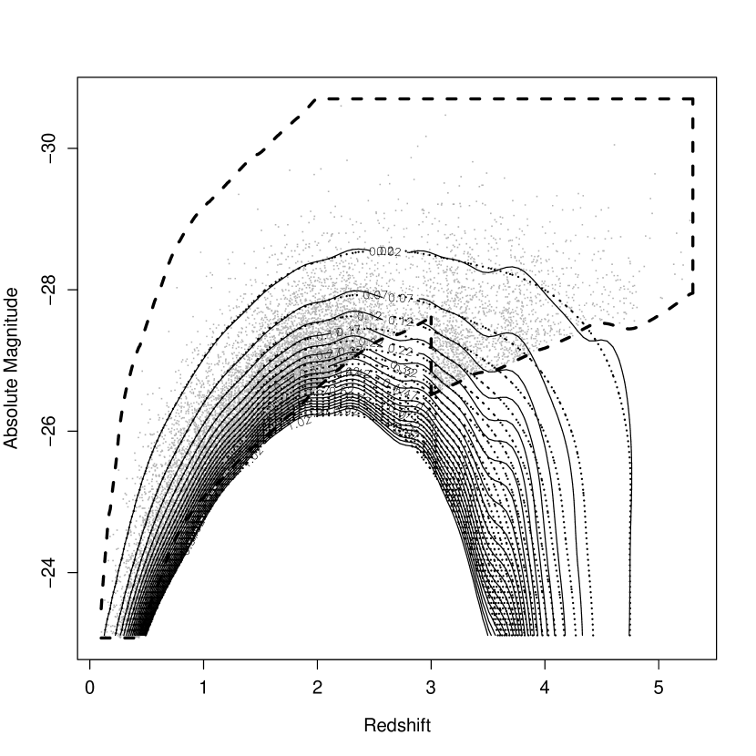
Figure 6: Estimates of the bivariate density. The contours are lines of constant density, with the estimate normalized to integrate to one over the observable (dashed) region. Thus, it is possible to estimate the number of quasars in a particular subset of $(z,M)$-space by integrating this function over that subset, multiplying by the observed count, and then dividing by the fraction of the sky covered by this survey. The solid contours are found using $\lambda_{z}=0.05$ and $\lambda_{M}=0.17$, which were the values of that minimized LSCV. Note the irregularity in the estimate at $z\approx 3.5$. This can be traced to similar fluctuations in the selection function. Another estimate was obtained by keeping $\lambda_{z}=0.05$ for $z\leq 2.0$, but using $\lambda_{z}=0.15$ for $z>2.0$, and is shown as the dotted contours. Using the larger bandwidth smooths out some of these artifacts.

Figure 6 shows, using the solid contours, the estimate of the quasar density (two-dimensional luminosity function) as a function of $z$ and $M$, when $\lambda_{z}=0.05$ and $\lambda_{M}=0.17$. This estimate is normalized to integrate to one over the entire dashed (observable) region. Recall from §3.3 that this is the form which the algorithm provides. Fortunately, this is the ideal form for the estimate. The (effective) count of quasars in the surveyed region is $n_{\mbox{\tiny eff}}=16858.51$ and the survey covers $1622\>\mbox{deg}^{2}$. Thus, the quasar count in a region $R$ of $(z,M)$ space can be estimated using

$$n_{\mbox{\tiny eff}}\left(\frac{\left(180/\pi\right)^{2}}{1622}\right)\left[\int_{R}\widehat{\phi}\!\left(z,M\right)dz\>dM\right].$$ (46)

The estimate of $\theta$ is $-0.41$, with a standard error of 0.03. Although it is not possible to assign physical significance to this value for $\theta$, it is clear that the possibility that $\theta=0$ is ruled out, and hence there is very strong evidence for evolution of the luminosity function with redshift.

This estimate has an apparent irregularity in the shape of the density estimate for $z\approx 3.5$. (Note the “bumps” in the solid contours for all values of $M$ at $z\approx 3.5$.) Quasars of this redshift are given larger weight due to interference from stars of spectral type G and K. Although it is not possible to be certain, it appears that the weighting may not be sufficiently accurate for the quasars. The weights may be underestimated leading to a corresponding dip in the density estimate. The bandwidth ($\lambda_{z}$) is sufficiently small to pick up this artifact. In fact, LSCV forces the bandwidth to be small enough so it can model this feature. It is hoped that in future work the uncertainty in the weights can be incorporated into LSCV. For comparison, another estimate was constructed using $\lambda_{z}=0.15$ for local models centered on redshift values larger than 2.0, while still using $\lambda_{z}=0.05$ for $z\leq 2.0$. This estimate is shown as the dotted contours. The increased smoothing removes the artifact.

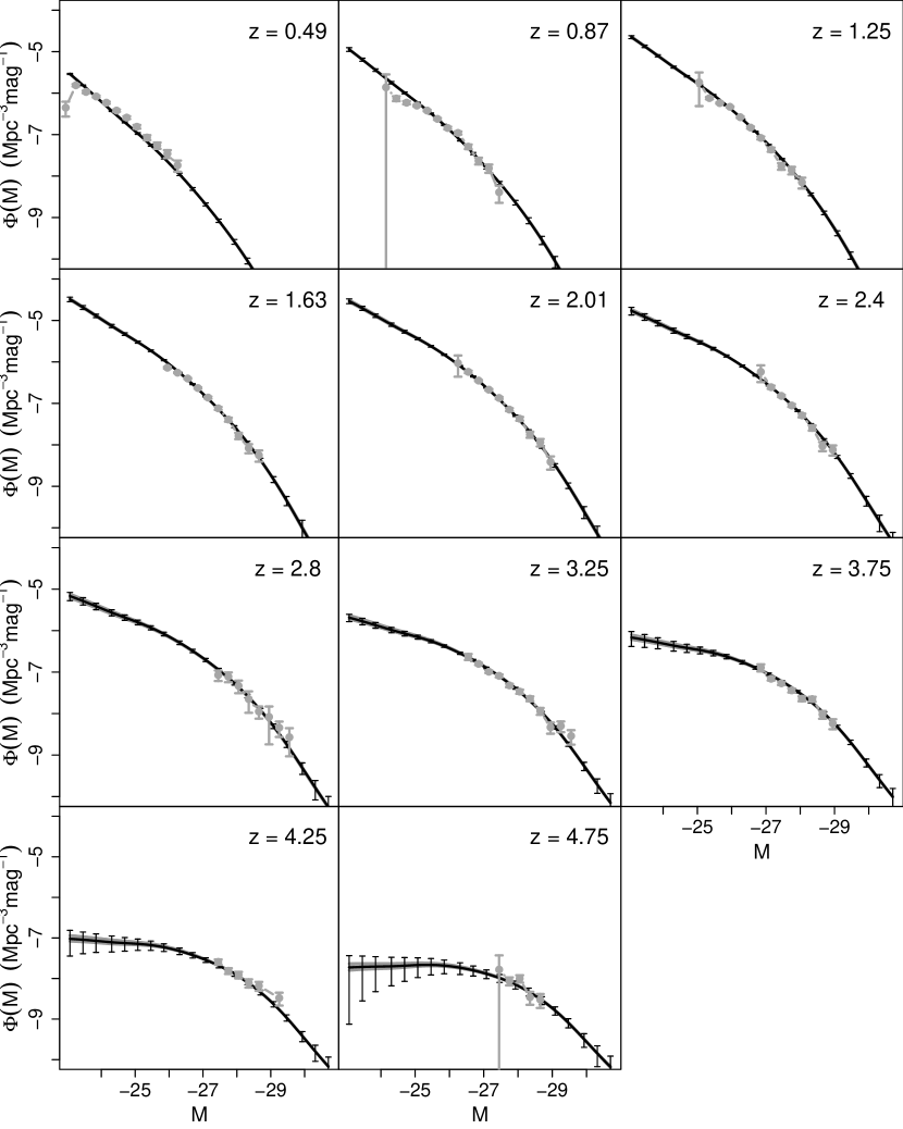
Figure 8: Estimates of the luminosity function at different redshifts (dark solid lines and error bars), compared with estimates from Richards et al. (2006) (light solid lines and error bars). These are cross-sections of the estimate shown in Figure 6, using $\lambda_{z}=0.05$ and $\lambda_{M}=0.17$ (the solid contours). Error bars represent one standard error and account for statistical errors only. Eight additional estimates were found by perturbing $\lambda_{z}$ and $\lambda_{M}$ by $\pm 0.01$. These estimates are shown as the gray curves (only visible at $M>-25$ and $z\geq 3.75$).

Figure 7 shows the estimated count of quasars with $M<-23.075$ as a function of redshift. As in Figure 6, the solid curve is the estimate with the LSCV-optimal bandwidths, and the dashed estimate is found using the increased smoothing. Figure 8 shows quasar counts as a function of absolute magnitude at a collection of redshift values. Comparisons are made with the estimates given in Richards et al. (2006) which were found using the bin-based method of Page & Carrera (2000). The error bars in both Figures 7 and 8 are one standard error, but represent statistical errors only. The error bars do not account for incorrect specification for the parametric form ${\bf h}$. But, if there is bias from the incorrect specification of ${\bf h}$, the binned estimates must share these biases. This would be surprising since, while having higher variance, estimates constructed from binning do not make assumptions regarding the evolution of the luminosity function, and hence a well-constructed estimate should be approximately unbiased.

Figure 8 also provides insight into the sensitivity of the estimate to the bandwidth choice. It would be of great concern if small changes in bandwidth led to significant changes in the estimate. To explore this, eight additional estimates were constructed using every possible combination of $\lambda_{z}\in\{0.04,0.05,0.06\}$ and $\lambda_{M}\in\{0.16,0.17,0.18\}$. The results are shown as gray curves in each plot of Figure 8, but are only visible at $M>-25$ and $z\geq 3.75$. The fluctuations are small relative to the size of the error bars. Clearly, the estimates are insensitive to these perturbations.

5.2 Simulation Results

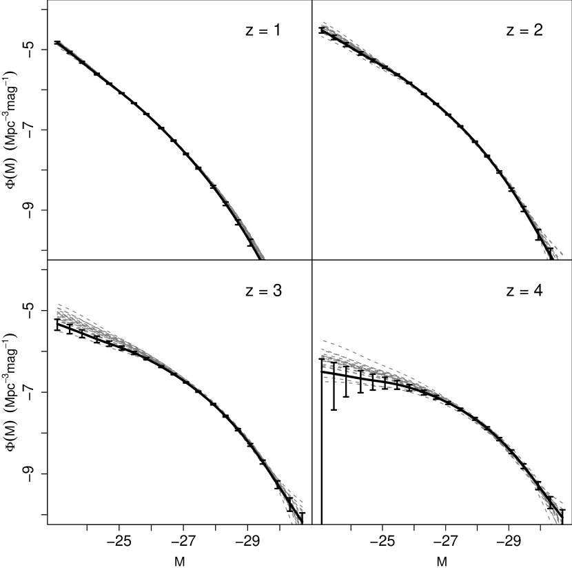
Figure 9: Results from simulations. The solid curve is the truth, and the dashed curves are the estimates from each of the 20 simulations. The error bars are one standard error, and found by averaging (in quadrature) the error bars over the 20 simulations.

Simulations were performed to further explore the behavior of the estimator. For these, the estimate shown in the dotted contours in Figure 6 is taken to be the true bivariate density; the truncation region is unchanged. The idea is to ask the following: If the truth were, in fact, the estimate found here, would this method be able to reach a good estimate of the density under identical conditions (same sample size and truncation region)? Hence, the new data sets were simulated consisting of 16,589 $(z,M)$ pairs within the observable region. The first of these data sets was utilized to find the optimal smoothing parameters; these were found to be $\lambda_{z}=0.06$ and $\lambda_{M}=0.16$. Each of the other 19 data sets was analyzed using these values, so that these simulations also provide insight into the adequacy of this approach to bandwidth selection. Figure 9 shows the results from the simulations by comparing estimates of the cross-sections of the estimates $\widehat{\phi}$ at four different redshifts. Each dashed curve is an estimate from one of the 20 data sets. The solid curve is the truth. These results show strong agreement between the estimates and the truth over the regions where data are observed. There is some bias in the tails, but this is in regions far from any observable data. In addition, these simulations provide strong evidence that the estimates of the standard errors are accurate: The variability in the estimates is comparable to the size of the error bars.

6 Summary

The semiparametric method described here is a strong alternative to previous approaches to estimating luminosity functions. The primary advantage is that it allows one to estimate the evolution of the luminosity function with redshift without assuming a strict parametric form for the bivariate density. Instead, one only needs to specify the parametric form for a term which models the dependence between redshift and absolute magnitude. Future work will focus on specifying a physically-motivated form for this parametric portion, but the results from the analysis of a sample of quasars reproduce well those from Richards et al. (2006) while only assuming a simple, first-order approximation to the dependence. Other portions of the bivariate density are modeled nonparametrically, and are functions of smoothing parameters. Using least-squares cross-validation, these smoothing parameters can be chosen in an objective manner, by minimizing a quantity which is a good approximation to the integrated mean squared error. Results from simulations show that, with a data set of this size, the method is indeed capable of recapturing the true luminosity curves under the truncation observed in these cosmological data sets.

7 Appendix

Appendix A M-estimators

The procedure described in §3 can be fit into a general class of statistical estimators called M-estimators. In the simplest case, a M-estimator for a parameter is constructed by maximizing a criterion of the form

$$\widehat{}\mbox{\boldmath$\beta$}_{\mbox{\tiny M}}\equiv\mathop{\rm arg\,max}_{\mbox{\tiny\boldmath$\beta$}\>\in\Theta}\left[\sum_{j=1}^{n}\varphi\!\left(\mbox{\boldmath$\beta$},X_{j}\right)\right]$$ (A1)

where $(X_{1},X_{2},\ldots,X_{n})$ are the observed data, assumed to be realizations of independent, identically distributed random variables and $\beta$ is the parameter to be estimated. The function $\varphi$ is some criterion. For example, in the case of finding the maximum likelihood estimate of $\beta$, the function $\varphi(\mbox{\boldmath$\beta$},x)=\log f_{\mbox{\tiny\boldmath$\beta$}}(x)$, where $f_{\mbox{\tiny\boldmath$\beta$}}$ is the density corresponding to parameter $\beta$. Most least squares problems can be stated as M-estimators. Standard theory for M-estimators can be applied to obtain an approximation to the distribution of $\widehat{}\mbox{\boldmath$\beta$}_{\mbox{\tiny M}}$, which can then be used to find standard errors and form confidence intervals.

In the case at hand, $X_{j}$ is the pair $(z_{j},M_{j})$, $\mbox{\boldmath$\beta$}=({\bf f},{\bf g},\theta)$, and

$$\varphi\!\left(\mbox{\boldmath$\beta$},X_{j}\right) \equiv \sum_{u\in{\cal G}}K^{*}\left(z_{j},u,\lambda\right){\bf a}_{u}\!\left(z_{j}\right)\>+\sum_{v\in{\cal G}}K^{*}\left(M_{j},v,\lambda\right){\bf b}_{v}\!\left(M_{j}\right)+{\bf h}\!\left(z_{j},M_{j},\theta\right)$$ (A2)

$${}-\int_{\cal A}\exp\!\left(h\!\left(z,M,\theta\right)\right)\left[\sum_{v\in{\cal G}}K^{*}\!\!\left(M,v,\lambda\right)\exp\!\left({\bf b}_{v}\!\left(M\right)\right)\right]\left[\sum_{u\in{\cal G}}K^{*}\left(z,u,\lambda\right)\exp\!\left({\bf a}_{u}\!\left(z\right)\right)\right]dM\>dz.$$

See Schafer (2006) to see the derivations of the approximate distribution for the estimator in this case.

The M-estimator could be generalized to the following:

$$\widehat{}\mbox{\boldmath$\beta$}_{\mbox{\tiny MW}}\equiv\mathop{\rm arg\,max}_{\mbox{\tiny\boldmath$\beta$}\>\in\Theta}\left[\sum_{j=1}^{n}w_{j}\varphi\!\left(\mbox{\boldmath$\beta$},X_{j}\right)\right]$$ (A3)

where $w_{j}>0$ is the weight given to the $j^{th}$ observation. This allows for easy incorporation of the selection function into the analysis. The statistical theory for this weighted M-estimator is a simple extension of that for the standard M-estimator.

Figure 4: An illustration of bandwidth selection by minimizing LSCV. The true density is the Gaussian with mean zero and variance one, and a sample of size 100 is used in the estimation. The chosen bandwidth is 1.25. The plot on the right shows how the optimal bandwidth yields an estimate (dashed line) near to the truth (solid line), while choosing the bandwidth too small (dash/dot line) or too large (dotted line) leads to poor estimates.

Figure 5: LSCV as a function of $\lambda_{z}$ and $\lambda_{M}$ for the analysis of the quasar data. Each dot represents a $(\lambda_{z},\lambda_{M})$ combination for which LSCV was calculated. The criterion is minimized when $\lambda_{z}=0.05$ and $\lambda_{M}=0.17$.

Figure 7: Estimates of the luminosity function as a function of redshift, integrated over absolute magnitudes less than -23.075. The solid curve is the estimate using $\lambda_{z}=0.05$ and $\lambda_{M}=0.17$. The depicted error bars are for this estimate and represent one standard error; these account for statistical errors only. The dashed curve is the smoother estimate found by keeping $\lambda_{z}=0.05$ for $z\leq 2.0$, but using $\lambda_{z}=0.15$ for $z>2.0$.

References

- Boyle et al. (2000) Boyle, B., Shanks, T., Croom, S., Smith, R., Miller, L., Loaring, N., and Heymans, C. 2000, MNRAS, 317, 1014
- Choloniewski (1986) Choloniewski, J. 1986, MNRAS, 223, 1
- Efron & Petrosian (1999) Efron, B. & Petrosian, V. 1999, J. Am. Stat. Assoc., 94, 824
- Efstathiou (1988) Efstathiou, G., Ellis, R., Peterson, B. 1988, MNRAS, 232, 431
- Felten (1976) Felten, J. 1976, ApJ, 207, 700
- Hall (1983) Hall, P. 1983, Ann. Stat., 11, 1156
- Hjort & Jones (1996) Hjort, N. & Jones, M. 1996, Ann. Stat., 24, 1619
- Jackson (1974) Jackson, J. 1974, MNRAS, 166, 281
- Loader (1996) Loader, C. 1996, Ann. Stat., 24, 1602
- Lynden-Bell (1971) Lynden-Bell, D. 1971, MNRAS, 155, 95
- Maloney & Petrosian (1999) Maloney, A., & Petrosian, V. 1999, ApJ, 518, 32
- Nicoll & Segal (1983) Nicoll, J. & Segal, I. 1983, A&A, 118, 180
- Page & Carrera (2000) Page, M. and Carrera, F. 2000, MNRAS, 433
- Qin & Xie (1999) Qin, Y.-P., & Xie, G.-Z. 1999, A&A, 341, 693
- Richards et al. (2006) Richards, G., et al. 2006, ApJ, 131, 2766
- Rudemo (1982) Rudemo, M. 1982, Scan. J. of Stat., 9, 65
- Sandage et al. (1979) Sandage, A., Tammann, G., & Yahil, A. 1979, ApJ, 232, 352
- Schafer (2006) Schafer, C. (2006) Submitted. Available as CMU Dept. of Stat. Tech Report #842 http://www.stat.cmu.edu/tr/tr842/tr842.html
- Schmidt (1968) Schmidt, M. 1968, ApJ, 151, 393
- Stone (1984) Stone, C. 1983, Ann. Stat., 12, 1285
- Takeuchi et al. (2000) Takeuchi, T., Yoshikawa, K., & Ishi, T. 2000, ApJS, 129, 1
- Willmer (1997) Willmer, C. 1997 AJ, 114, 898
- Wang (1989) Wang, M.-C. 1989, J. of Amer. Stat. Assoc. 84, 742
- Wasserman et al. (2001) Wasserman, L., Miller, C., Nicol, R., Genovese, C. Jang, W., Connolly, A., Moore, A., & Schneider, J. 2001, astro-ph/0112050
- Woodroofe (1985) Woodroofe, M. 1985, Ann. Stat., 13, 163
- York et al. (2000) York, D. 2000, AJ, 120, 1579