The Compact, Conical, Accretion-Disk Warm Absorber of the Seyfert 1 Galaxy NGC 4051 and its Implications for IGM-Galaxy Feedback Processes

Abstract

Using a 100 ks XMM-Newton exposure of the well studied, low black hole mass (M${}_{BH}=1.9\times 10^{6}$ M_⊙) Narrow Line Seyfert 1 NGC 4051, we show that the time evolution of the ionization state of the X-ray absorbers in response to the rapid and highly variable X-ray continuum constrains all the main physical and geometrical properties of an AGN Warm Absorber wind. We use a technique that takes advantage of the complementary high resolution in the RGS grating data and the high S/N in the EPIC CCD data. The absorber consists of two different ionization components, with a difference of $\approx$ 100 in ionization parameter, and a difference of $\approx$ 5 in column density. By tracking the response in the opacity of the gas in each component to changes in the ionizing continuum, we were able to constrain the electron density of the system. We find $n_{e}=(5.8-21.0)\times 10^{6}$ cm^-3 for the high ionization absorber and $n_{e}>$8.1$\times$10⁷ cm^-3 for the low ionization absorber. Combined with the X-ray luminosity and ionization parameter, these densities require that the high and low ionization absorbing components of NGC 4051 must be compact, at distances 0.5-1.0 l-d (2200 - 4400R_s) and $<$ 3.5 l-d ($<~{}15800$R_s) from the continuum source, respectively. This rules out an origin in the dusty obscuring torus, as the dust sublimation radius is at least an order of magnitude larger ($\sim$12 l-d), and also rules out an association with the low ionization H$\beta$ emitting broad emission line region (radius 5.6 l-d). An accretion disk origin for the warm absorber wind is strongly suggested, and an association with the high ionization, HeII emitting, broad emission line region (radius $<$2 l-d) is possible. The warm absorber has a relative thickness, $\Delta R/R\sim$ 10% - 20%, and the two detected phases are consistent with pressure equilibrium, which suggests that the absorber consists of a two phase medium. A radial flow in a spherical geometry is unlikely, and a conical wind geometry is preferred. The implied mass outflow rate from this wind, can be well constrained, and is $2-5$ % of the mass accretion rate. If the mass outflow rate scaling with accretion rate is representative of all quasars, our results imply that warm absorbers in powerful quasars are unlikely to produce important evolutionary effects on their larger environment, unless we are observing the winds before they get fully accelerated. Only in such a scenario can AGN winds be important for cosmic feedback.

1 Introduction

Feedback from quasars and their less luminous cousins Active Galactic Nuclei (AGN) - via radiation, highly directional relativistic jets, and slower wide angle winds - has been recognized as a potentially crucial input to cosmology (e.g. Ciotti & Ostriker 1997; Magorrian et al. 1998; Gebhardt et al.; 2000; Ferrarese & Merritt 2000; Elvis et al. 2002; Hopkins et al. 2005; Nulsen et al. 2005). However, while the first two mechanisms have been known for a long time, the prevalence and strength of quasar winds is only now becoming clear. Without a firm physical grasp of the wind mechanisms, their importance must remain speculative. The most fundamental question is where do quasar winds originate? Proposals span a factor $>~{}10^{6}$ in radius and include (a) the Narrow Line Region(e.g. Kinkhabwala et al. 2002; Ogle et al. 2004), (b) the inner edge of the ‘obscuring torus’ (Krolik & Kriss 2001) , and (c) the accretion disk itself (Elvis 2000). Discriminating among these widely different scales ($\sim 10$ kpc to $\sim 0.001$ pc) requires the independent determination of a quantity which is not directly observable: the electron density $n_{e}$ of the outflowing material, which then gives the distance $R$ from the central ionizing source.

Ionized absorption outflows (Warm Absorbers: WA) have been observed in the Ultraviolet (UV) and X-ray spectra of $\lower 2.15277pt\hbox{$\;\buildrel>\over{\sim}\;$}50$ % of Seyfert 1s (e.g. Crenshaw, Kraemer & George 2003) and quasars (Piconcelli et al. 2005), with line of sight velocities of the order of a few hundreds to $\sim 2000$ km s^-1. Such high detection rates, combined with evidence for transverse flows (Mathur et al. 1995; Crenshaw, Kraemer & George 2003, Arav 2004) suggest that WAs are actually ubiquitous in AGN, but become directly visible in absorption only when our line of sight crosses the outflowing material. Recent efforts to understand WAs have concentrated on the accurate spectral modeling of the hundreds of bound-bound and bound-free transitions directly visible in the time-averaged, high signal-to-noise (S/N), high-resolution X-ray spectra of nearby Seyferts (e.g. Krongold et al. 2003; Netzer et al. 2003). While these studies have been decisive in showing that there are just a few distinct physical components in these outflows, only average estimates of the product $(n_{e}R^{2})$ could be derived from such time-averaged spectral analyses. This is due to the intrinsic degeneracy of $n_{e}$ and $R$ in the equation that defines the two observables: the average ionization parameter of the gas $U_{x}=Q_{x}/(4\pi R^{2}cn_{e})$ and the luminosity of ionizing photons $Q_{x}$.

It was recognized some years ago (Krolik & Kriss 1995; Reynolds et al. 1995; Nicastro et al. 1999) that there is an unambiguous method to remove this degeneracy: by monitoring the response of the ionization state of the gas in the wind to changes of the ionizing continuum, it is possible to measure the density of the gas and, hence, its distance from the ionizing source. Since the ionization parameter depends linearly on the ionizing flux, it needs to be assumed that the density and location of the absorber do not change on the typical timescales of variability. This method has been applied in the past to constrain the location of the absorber. For instance Reynolds et al. (1995) applied this technique to ASCA data of MCG -6-30-15 and concluded that the absorber should be located at subparsec distances from the central source. Nicastro et al. (1999) concluded, based on ROSAT data, that the absorber in NGC 4051 should be located at a distance $\sim$3 l-d from the supermassive black hole (§5.4). Netzer et al. (2002) used Chandra and ASCA data of NGC 3516 to place the absorber at subparsec distances from the ionizing source. Netzer et al. (2003) and Behar et al. (2003) used the lack of variability in timescales of days for the warm absorber in NGC 3783, and set a lower limit $\sim$1-3 pc on the distance of the warm absorber, while Krongold et al. (2005) reported variations in this source on timescales $\sim$ 1 month, and placed the absorber within 6 pc. Reeves et al. (2004) further reported variability of the Fe XXV and XXVI absorption lines in NGC 3783 and located the gas within 0.1 pc from the supermassive black hole.

Other methods have also been used to measure the location of the absorbing gas. Kaastra et al. (2005) reported the detection of an O V absorption line arising from a meta-stable level in Mrk 279, and used it to constrain the density of the gas. These authors placed the absorber at distances between 1 light week to few light months from the central source. Gabel et al. (2005) detected meta-stable absorption from C III in one of the three absorption components present in the UV data of NGC 3783 (the highest velocity component) and place this UV absorber at a distance of 25 pc. He also concluded that the gas producing the other two UV velocity components must be located anywhere within 25 pc (the UV absorbers have been associated with the X-ray absorber, Gabel et al. 2003). Such different determinations of the absorber location may be reflecting simply the fact that we are observing a large scale outflow, with different components. However, we note that to determine the origination radius of the WA winds it is always the smallest radius found the one that gives the strongest constraint.

Here, we follow the response of the absorbing gas in NGC 4051 to rapid changes in the continuum, using high S/N XMM-Newton data of this source, in combination with a detailed multi-phase ionized absorber spectral model (PHASE, Krongold et al. 2003) and the constraints provided by time-evolving photoionization (Nicastro et al. 1999), to produce an accurate determination of the absorber density and distance. NGC 4051 is a low luminosity ($L_{bol}=2.5\times 10^{43}$ ergs s^-1, Ogle et al. 2004), low black hole mass (M${}_{BH}=1.9\times 10^{6}$ M_⊙, Peterson et al. 2004) AGN, which varies rapidly ($\sim$ 1 hour) and with large amplitude (a factor $\sim$10; McHardy et al. 2004). We use a novel technique that takes great advantage of the complementary high resolution in the RGS grating data and the high S/N in the EPIC CCD data, to effectively track the changes in the WA properties over small time scales.

2 The Variable Spectrum of NGC 4051

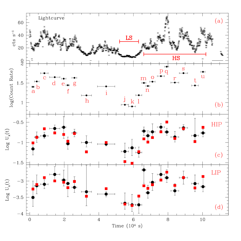
Figure 1: Panel (a): Lightcurve of NGC 4051 in bins of 100 s. The high flux state (HS) and low flux state (LS) regions used for our analysis are labeled. Panel (b): Log of the count rate vs. time, for the 21 “flux states” used to study the variability of the warm absorber. Spectra were extracted for each of the 21 bins, with an exposure time given by the x error bars. Panel (c): Log of the Ionization parameter of the HIP (U${}_{x}^{HIP}$) as a function of time. For easy comparison with the continum level, the red squares represent the count rate in each bin shifted by an offset of -0.81. Panel (d): Log of the Ionization parameter of the LIP(U${}_{x}^{LIP}$). The red squares have an offset level of -3.05.

NGC 4051 was observed for $\sim$117 ks with the XMM-Newton Observatory, on 2001 May 16-17 (Obs. Id. 0109141401). The source varied by a factor of a few on timescales as short as 1 ks, and by a factor of $\sim$12 from minimum to maximum flux over the whole observation (see Fig. 1a). We retrieved the data from the XMM-Newton data archive and reprocessed the observations using the XMM Newton Science Analysis System (SAS v6.1.0).

The task epchain was used to obtain calibrated event lists for the EPIC-PN camera (Struder et al. 2001) which has a better calibration below 0.8 keV than EPIC-MOS. EPIC-PN operated in small-window mode with medium filters, ensuring a negligible level of pile-up. The last 14 ks of the observation had a background level significantly increased due to the presence of soft photons and these data were not included in our analysis. We reprocessed the RGS (den Herder et al. 2001) data and extracted spectra using the task rgsproc. Spectral modeling was carried out with the Sherpa (Friedman, Doe, & Siemiginowska 2001) package of the CIAO software (Fruscione 2002).

3 Modeling the Spectra of NGC 4051

3.1 Constraining the absorber properties

We modeled the RGS continuum with a complex model consisting of a power-law plus two thermal components attenuated by absorption due to our own Galaxy ($N_{H}=1.31\times 10^{20}$ cm^-2, Elvis, et al. 1989). Strong residuals were evident in the spectrum ($\chi^{2}=2607/1842$ d.o.f.). Narrow emission lines have been reported in the spectrum of NGC 4051 from a 2002 November XMM-Newton observation, when the source was in a very low state (Pounds et al. 2004). The lines have constant intensity (Pounds et al. 2004), so we included in our models the strongest 8 emission lines with the parameters fixed at the 2002 November values (Table 1), which we determined fitting the RGS data of that observation (the analysis of this observation will be presented in the future). Our model for the total RGS 2001 observation was statistically better than the previous one without lines ($\chi^{2}=2456/1819$ d.o.f.), confirming the presence of these features. However, the spectrum still showed large residuals similar to those produced by an ionized absorber. In particular, strong residuals were present in regions consistent with strong absorption lines by H-like and He-like ions of O, N, and C.

We then added to our model an ionized absorbing component using PHASE (Krongold et al. 2003), a spectral code that has proven highly successful in modeling absorption by photoionized gas. PHASE has three free parameters for each component: the ionization parameter, $U_{X}$, in the 0.1 keV-10 keV range (Netzer 1996); the equivalent H column density, N_H, and the line of sight outflow velocity of the absorber, $v$. A fourth parameter, the turbulent velocity of the gas, was set to 300 km s^-1 (see Krongold et al. 2003 for details). Throughout the paper we have assumed solar elemental abundances for the absorbing gas (Grevesse et al. 1993). The inclusion of this ionized absorbing component significantly improved our fits ($\chi^{2}=2116/1816$ d.o.f.). An F-test indicates that the absorber is required at a significance level of 99.99%. However, this model still left weak residuals in the region between 12-14 Å where Fe L-shell lines are intense, suggesting the possible presence of a second ionization component, as has been found for other Seyfert 1 galaxies (e.g. Steenbrugge et al. 2003; Krongold et al. 2003; Blustin et al. 2005, Costantini et al. 2006).

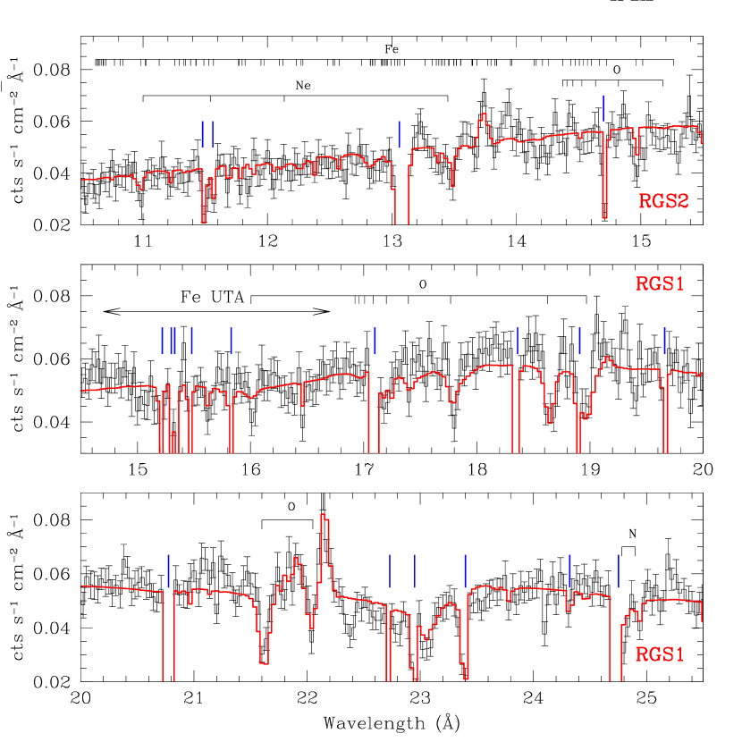
Figure 2: Two absorber best-fit model over the full time integrated RGS sepectrum. Absorption lines are labelled according to the element producing them. The blue lines mark instrumental features.

We thus included a second ionization component in our model and re-fit the data. This model (reported in Table 2) fit better ($\chi^{2}=2033/1813$ d.o.f.) than the one absorber model. An F-test shows that the second absorbing component is required at a significance level of 99.99%. This is consistent with results from other analyses of this source where two absorbing components were also found (e.g. Pounds et al. 2004; Ogle et al. 2004). One of the two absorbing components the low ionization phase (LIP), has an ionization parameter two orders of magnitude smaller than the other component, the high ionization phase (HIP). We will further show in §6 that these two components do not represent just a sufficient fit to the absorber (that could instead be formed by a continuous radial distribution of ionization parameters), but that they are two genuinely distinct absorbing phases. Figure 2 shows the RGS spectrum with our best-fit model.

Finally, we note that, in modeling the same NGC 4051 spectrum, Pounds et al. (2004) also used a description of the continuum with two thermal components (Uttley et al. 2004 also required two thermal components for their analysis of the EPIC data of NGC 4051). Ogle et al. (2004) found, however, that conventional continuum emission processes cannot explain the “soft excess” in the spectrum of NGC4051. However, we note that Ogle et al. did not explore the possibility of two blackbodies in their models. Instead, they used relativistic emission lines of the entire O VIII series plus radiative recombination to describe the continuum. The nature of the soft excess observed in the X-ray spectra of Seyfert galaxies is still not well understood. In the case of NGC 4051, we note that the data is not sufficient to decide between two blackbodies and relativistic emission by O VIII. Both models provide a good description of the continuum emission, and we point out that using one or the other representation of the continuum has no effect on the results found here for the ionized absorber in NGC 4051.

3.1.1 On the Presence of Broad Emission Lines

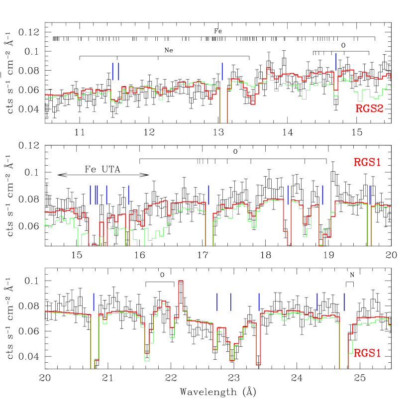
Figure 5: High State (HS) best-fit model plotted over the RGS High State data. Absorption lines are labelled according to the element producing them. The blue lines mark instrumental features. The green line represents the best fit model obtained for the fit of the Low State RGS spectrum for comparison (the LS best-fit model).

Ogle et al (2004) reported the presence of two broad emission lines (O VII $2p-1s$ [r] and C VI $2p-1s$ [Ly_α]), presumably from the Broad Emission Line Region, in the spectrum of NGC 4051. There is indeed an excess of flux with respect to the fitted continuum in our models, in the ranges 21-22 Å, and 33-34 Å (see also Figure 5 in Ogle et al. 2004), where these lines should be present. We thus added two Gaussians to our model and, according to an F-test, found that these broad features are required with a 99.9% level of confidence. However, despite this large statistical significance, the lines rise only 5-10% above the continuum level which makes their detection unreliable. Possible residual calibration uncertainties, among other effects, could in principle produce similar features. To further test whether the emission lines are real detections or not, we looked for possible emission by the intercombination and forbidden O VII lines. According to Porquet & Dubau(2000), in photoionized plasma, even at electron densities $\sim 10^{10}$ cm^-3 the O VII forbidden line should be $\approx$3 times brighter than the resonance line. Only at densities $\sim 10^{12}$ cm^-3 the forbidden line is significantly suppressed (to about half the brightness of the resonance line). However, at these densities, the intercombination lines become 3-4 times brighter than the resonance line. We thus attempted to fit an O VII triplet composed of 3 broad Gaussians, imposing these restrictions in the fluxes of the lines. The data is not consistent with such emission line ratios, implying no significant contribution to the emission by the forbidden and intercombination lines (as can be seen at wavelengths larger than 22 Å, where the low energy wing of the forbidden line should be present). In order for the resonance line to dominate the emission, densities much larger than $10^{12}$ cm^-3 are required. However, these lines also need a high ionization state for the emitting gas (similar to the one of the HIP), and such large densities would locate the gas within the horizon of events (see §5.2). Thus, it is unlikely that the flux excess between 21 and 22 Å is due to a broad O VII line. Furthermore, 5-10% flux excesses can be found in other regions of the spectra where broad emission lines are not expected. We conclude that the present data is not suitable for detecting such broad and weak emission features.

3.2 Analysis of Chandra Data of NGC 4051

From Figure 2, we note that the the HIP is not as evident (visually) in the data as the LIP due to several instrumental features in the RGS detector that lie very close to the expected absorption lines, compromising their identification. In addition, in the region between 10 and 14 Å  where most of the absorption features of the HIP lie, the RGS S/N is limited. Only the RGS 2 detector is in operation in this region, while at higher energies, where more HIP absorption lines are expected, the sensitivity of the RGS declines rapidly, making the detection of this component difficult.

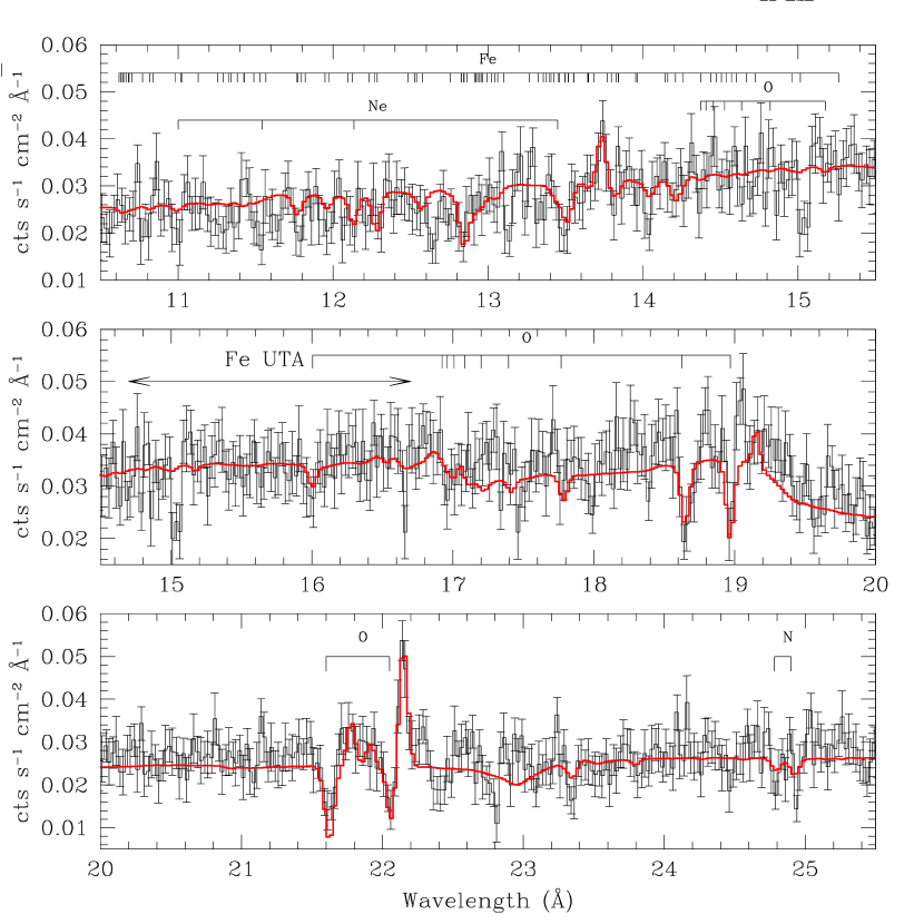
Figure 3: Two absorber best-fit model over the Chandra HRC-LETG sepectrum. Absorption lines are labelled according to the element producing them. The strong absorption line at 15 Å, corresponding to an Fe XVII transition, is clearly underpredicted by our model.

As noted by Williams et al. (2006), the gratings on board Chandra have a notably better sensitivity for detecting individual narrow absorption lines. Thus, to further confirm the presence of the HIP we retrieved and analyzed a $\sim 100$ ks Chandra HRC-LETG observation of NGC 4051 (a full analysis of these data will be presented in a forthcoming paper), carried out in July 2003, for which the source flux is similar to that during the XMM observation (the flux in the 6-35 Å range was $\approx 3.7\times 10^{-11}$ erg cm^-2 s^-1 during the XMM observation and $\approx 4.4\times 10^{-11}$ erg cm^-2 s^-1 during the Chandra observation). We modeled these data following the same approach we used with the RGS data. Our model clearly indicated the presence of the same two components found in the RGS data, with similar column densities and outflow velocities. The ionization parameters measured for both components were also indistinguishable in the two spectra, implying an absorber close to photoionization equilibrium (log U${}_{x}^{LIP}$(Chandra) = -3.14; log U${}_{x}^{HIP}$(Chandra)$~{}=~{}-0.79$). Figure 3 presents our model over the Chandra data. The presence of both the LIP and HIP components is evident in the spectrum, and an F-test gives a significance larger than 99.99% for the presence of the second absorbing component (the HIP).

The LIP produces strong absorption features due to O VII (lines at 21.6 Å, 18.63 Å, 17.77 Å, 17.40 Å, and 17.20 Å) and OVI (line at 22 Å), as well as Fe M-shell absorption (the unresolved transition array or UTA, between 15 and 17 Å). The HIP produces absorption lines by O VIII (at 18.97 Å) , Ne IX-X (at 13.45 Å, 12.13 Å, 11.54 Å, and 11.00 Å), and Fe L-shell lines (between 10 and 15 Å), in particular by Fe XIX (intense lines at 13.80 Å, 13.64 Å, 13.55 Å, 13.52 Å, 13.50 Å, 13.46 Å and 13.42 Å), Fe XX (intense lines at 13.1 Å, 12.97 Å, 12.91 Å, 12.85 Å, 12.82 Å and 12.57 Å), and Fe XXI (most intense line at 12.28Å). We note that in both the RGS and LETG data there is a significant absorption line at 22.38$\pm$0.01 Å (EW$=3.5\pm 0.7$ mÅ) that is not reproduced by the model. This line can be identified with an O V transition not included in PHASE. The feature at 22.80$\pm$0.02 Å (EW$=1.9\pm 1.1$ mÅ) could be an absorption line produced by O IV also missing in PHASE, though this feature is marginally significant in the data.

3.3 Variability in the opacity of the ionized absorbers

To study the response of the absorbers to ionizing flux changes we extracted RGS spectra during a “low flux state” (hereafter LS) and a “high flux state” (hereafter HS). These states can be clearly identified in Figure 1a, and they correspond to a large variation in flux (by a factor $\sim 4.5$) over a short timescale ($\sim 5$ ks). Following the approach described in §3.1, we fit the LS and HS spectra of NGC 4051 separately, but fixing the equivalent H column densities and outflow velocities of the absorbers to the values obtained for the whole observation (Table 2). The best-fit ionization parameters of the two absorbing components (Table 3) vary between the LS and HS, indicating that there are spectral variations that can be fairly modeled as opacity changes between the two states. These changes in opacity were first noted and reported by Ogle et al. (2004) on this same data set, however, these authors did not model the time-dependence of the absorber as we do here.

For the LIP, the detected change in $U_{x}$ between the HS and LS RGS data is significant at the $3\sigma$ level (Table 3) and, within the errors, the change in ionization parameter is similar to the change in flux (factor $\sim$4.5). This strongly suggests that during the flux increase from the LS to the HS, this absorbing component reaches photoionization equilibrium with the ionizing source. For the HIP the statistics are poorer. However, even for this component a change in $U_{x}$ is suggested, though significant only at the $1.6\sigma$ level, and is consistent with the change in flux within the uncertainties, allowing this absorbing component too to be close to photoionization equilibrium. For the ionized absorbers to reach photoionization equilibrium in 5 ks they must be dense and thus close to the ionizing continuum source. We will quantify this statement in §5.

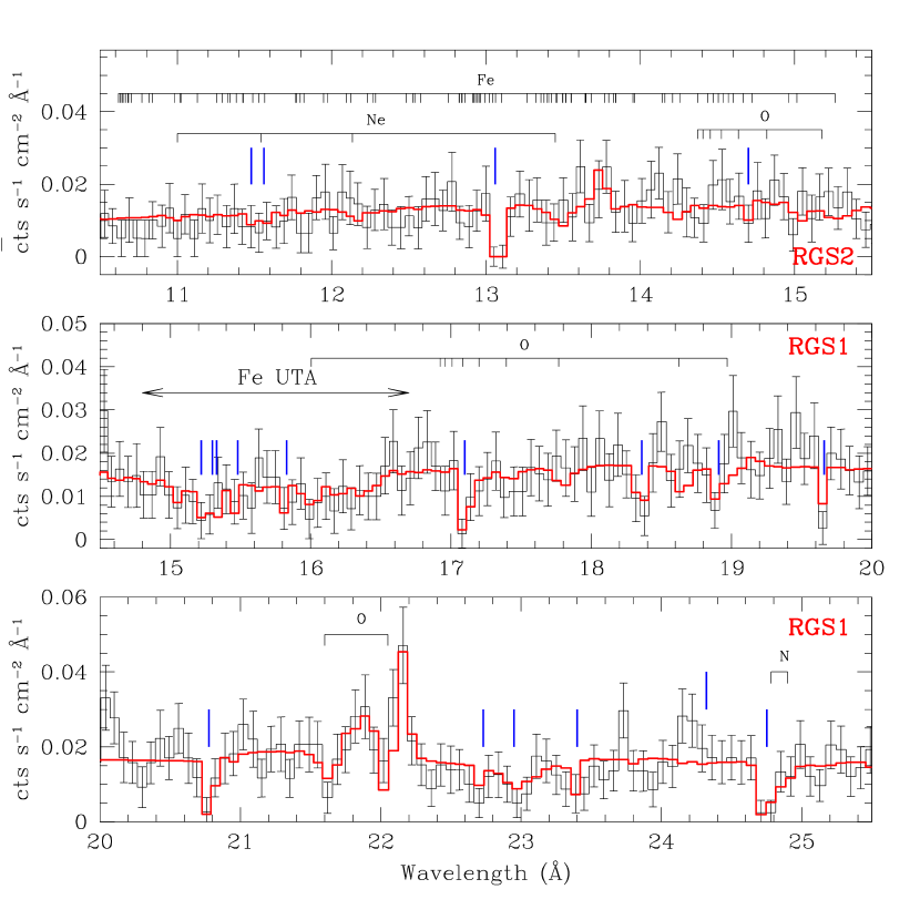
Figure 4: Low State (LS) best-fit model plotted over the RGS Low State data. Absorption lines are labelled according to the element producing them. The blue lines mark instrumental features.

The best fit model for the RGS LS is presented in Figure 4 and the best fit model for the RGS HS is in Figure 5 (in both Figs. the RGS data are binned to $\sim$55 mÅ per bin). It can be observed that the variations in the spectrum of NGC 4051 are indeed consistent with the changes expected for the WA. In particular, the spectral changes in the region between 15 and 18 Å can be interpreted as variations in the opacity of the gas composing the LIP, reflected in the broad feature produced by the Fe M-shell UTA absorption. This can be clearly seen in Figure 5 with the HS data by comparing the red line (the high state model) with the green line (the LS model). Between 10.5 and 15 Å changes for the HIP are expected, however these changes are less evident than those for the LIP, and weaker because of the numerous blends of Fe L-shell transitions arising from different charge states. This make the changes for this component harder to see by eye. However, comparing the LS and HS models in Figure 5, broad changes can be observed between 14 and 15 Å. Additionally, a clear variation in a semi-narrow feature is observed in the complex around 13.5 Å produced by several transitions of Fe XIX. Another semi-narrow feature where variation is suggested is the complex around 12.9 Å produced by several transitions of Fe XX.

We note that variations in narrow absorption features are not seen in the RGS spectra at a significant level mainly because of (1) the limited spectral resolution of the RGS (2.4 times broader FWHM than the LETG on board Chandra, Nicastro et al. 2007, in preparation) and (2) the low S/N ratio of the LS data. Then, in these data only the strongest absorption lines can be detected, but such lines are heavily saturated, and therefore they are not expected to vary significantly. In addition blending of weaker lines from different charge states, instrumental features in the RGS coinciding with some of the most promising absorption lines, and line absorption filling by nearby narrow emission lines complicate further the detection of variability in narrow features. We list some of the non-saturated, unblended, narrow absorption lines that are expected to vary, and are promising to be detected in high resolution data with much higher S/N (i.e. the data expected to be obtained with future X-ray missions like Constellation-X, Xeus or Pharos): For the HIP Ne X at 10.24 Å, O VIII at 14.82 Å, and 15.18 Å, Fe XVII at 10.77 Å, 11.02 Å, 11.13, 11.25 Å, 13.82 Å, 14.37 Å, and 15.26 Å are expected to be more prominent when the source is at flux levels similar to the one of the low state (LS). Fe XXI at 12.28 Å, is expected to be prominent during flux levels similar to the HS. For the LIP O VII at 17.20 Å and 17.40 Å, O VI at 22.03 Å, O V at 22.37 Å (not included in our models), and N VI at 24.90 Å are expected to be more prominent during the LS.

3.4 Modeling the EPIC data

Motivated by the suggested 3$\sigma$ and 1.6$\sigma$ variability seen with the RGS we analyzed the low resolution, but higher S/N, EPIC-PN spectrum of NGC 4051. The dominance of the broad UTA and Fe-L shell features in the RGS spectrum of the ionized absorber holds out the promise that this low resolution but higher S/N data could also constrain the changes in opacity of the absorber.

We modeled the EPIC-PN spectrum of the whole observation using the same spectral components used to model the RGS data (including a power-law plus two thermal components for the continuum, plus two ionized absorbers). We fit the EPIC spectrum leaving all parameters free to vary, except the outflow velocity and column density of each absorbing component, which were fixed to the best-fit RGS values. The best-fit parameters are listed in Table 1.

The ionization parameters derived from the EPIC data are fully consistent with those obtained independently from the RGS data. This result shows that when the velocities and column densities of ionized absorbers are constrained by high resolution data, the ionization parameter can be well modeled at CCD X-ray spectral resolution (see also Krongold et al. 2005b).

As a further check, we extracted EPIC-PN spectra from the same high (HS) and low (LS) states used for the RGS analysis (§3.3). The change in the opacity of the absorbers detected in the high resolution RGS spectra can also be detected (though not resolved) with the higher S/N of the CCD spectra. Quantitatively, the best-fit values of the ionization parameters are consistent with those derived from the high resolution data, for both absorbing components (HIP and LIP) and during both flux states (LS and HS, see Table 3). However, the values derived from the EPIC-PN data are more tightly constrained due to the higher S/N of the CCD data (with the velocity and column densities fixed at the RGS values). For the LIP, the EPIC data show opacity variations at a significance level $\sim 4.3\sigma$ (Table 3), confirming the RGS results that were significant only at a $\sim 3\sigma$ level, while for the HIP the significance level increases from the 1.6$\sigma$ level for the RGS data to a $\sim 3.5\sigma$ level (Table 3). For both components the models are consistent with the gas reaching photoionization equilibrium.

4 Following the time-variability of the ionized absorbers

Since NGC 4051 varies on typical timescales of a few ks (Fig. 1), the best constraints on the time dependence of the ionized absorbers, will come from spectra in time bins of similarly short duration. In light of the encouraging results with the EPIC-PN data, we then performed a more finely time-resolved spectral analysis, exploiting the better statistics of the EPIC-PN data, with the aim of constraining the opacity variations of the ionized absorbers on timescales as short as few ks. We extracted EPIC-PN spectra from 21 distinct continuum levels (a - u, see Fig. 1b), though for two intervals (d and i) the source varied significantly on timescales shorter than $\sim$2 ks, so these two are still only “time averaged spectra”. To improve the signal to noise ratio of the 21 spectra, we binned the pulse height data to have 15 original channels per bin.

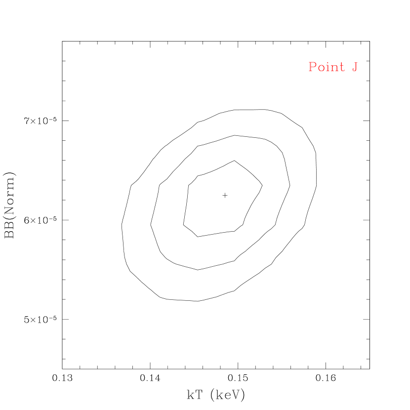
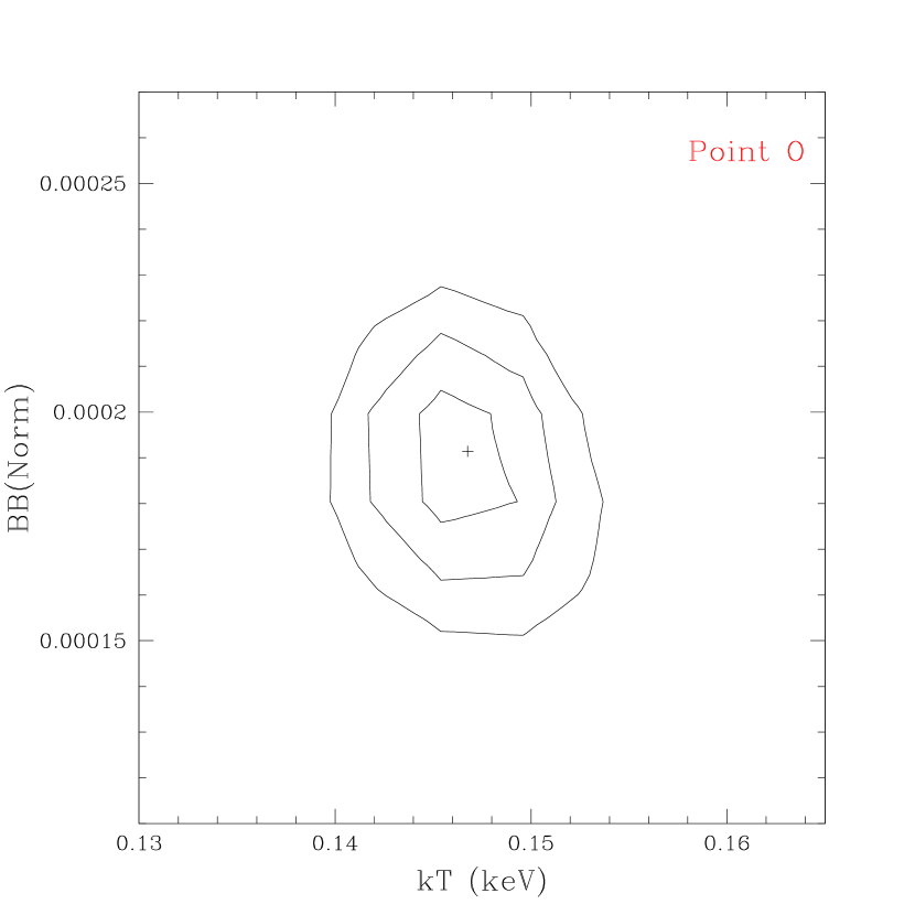
Figure 6: Blackbody temperature (kT=0.14 keV) vs. blackbody normalization confidence regions for two spectra with very different flux level (states j and o) showing no correlation between these quantities. The temperature of the blackbody is consistent with no change in the 21 spectra used in our analysis. The normalization is in L₃₉/(D₁₀)² units, where L₃₉ is the source luminosity in units of 10³⁹ erg s^-1 and D₁₀ is our distance to the source in units of 10 kpc.

For each spectrum, we again fit the continuum with a power law plus two blackbodies attenuated by both neutral absorption due to our own Galaxy, plus the eight most prominent (non-variable) emission lines (see §3.1). We also included two ionized absorbers in our models, as indicated by the high resolution spectra. We used the following approach: since there is evidence that the shape of the soft excess varies only in amplitude (see Fig. 6, and Pounds et al. 2004; Uttley et al. 2004), we required the temperatures of the two blackbody components to be the same for all 21 spectra. We also assumed that the two ionized absorbers did not change in N_H during the observation by fixing N_H to the same (best-fit) value in all the models. Physically, this is plausible as a the column density of the absorber has remained constant for several years (from the 2001 XMM-Newton observation to the 2003 Chandra observation). The fitted N_H values turned out to be consistent with the ones determined from the RGS data. The outflow velocity of each absorber was also assumed constant and was constrained to the best-fit RGS value. Thus, within the 21 individual spectra we left free to vary only: (1) the slope and amplitude of the power-law, (2) the amplitude of the two blackbody components, and (3) $U_{X}$ for each of the two absorbers. With only 3 free parameters, our fits are able to detect smaller changes in $U_{X}$.

For both absorbing components the derived $U_{X}$ values follow closely the source continuum lightcurve [compare panel (c) and (d) with panel (b) of Figure 1], clearly indicating that the gas is responding quickly to the changes in the ionizing continuum.

4.1 Testing the Photoionization Equilibrium Hypothesis

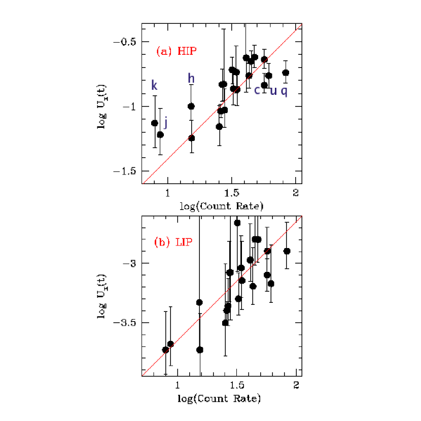
Figure 7: Log$U_{X}(t)$ vs. log of the source count rate (log$C(t)$), for the HIP (panel (a)) and the LIP (panel (b)). For most of the points of the HIP and for all points of the LIP, log$C(t)$ correlates with log$U_{X}(t)$ tightly. HIP and LIP are close to photoionization equilibrium. The solid red lines represents the photoionization equilibrium relation and determine the values of $n_{e}R^{2}$ for the two components to be 3.8$\pm 0.7\times 10^{37}$ cm^-1 for the HIP and 6.6$\pm 0.1\times 10^{39}$ cm^-1 for the LIP (see text for details).

To study more quantitatively how these changes are related to the changes in the continuum, we show in Fig.7a,b the log of the source count rate (log$C(t)$) vs. log$U_{X}(t)$, for the HIP [panel (a)] and the LIP [panel (b)]. For most of the points of the HIP and for all the points of the LIP (within 2$\sigma$), log$C(t)$ correlates with log$U_{X}(t)$ tightly. We then assume photoionization equilibrium and derive the quantity $(n_{e}R^{2})$ by fitting the equilibrium relationship $logU_{X}(t)=logQ_{X}(t)-log(4\pi cn_{e}R^{2})=log[(C(t)/S_{eff})\times(4\pi D^{2})]-log(4\pi cn_{e}R^{2})$, to the data points in Figure 7. In the above formula, $Q_{X}$ is the rate of 0.1-10 keV photons produced by the source, $(n_{e}R^{2})$ is the product between the electron density of the gas and the square of its distance from the ionizing source, $C(t)$ and $S_{eff}$ are the observed count rate and the instrument effective area in the 0.1-10 keV band, respectively, and $D=15.5$ Mpc (Shapley et al. 2001) is the distance to NGC 4051. We adopted a value of $S_{eff}\sim$260 cm², and performed a single parameter fit (i.e. we assumed $U_{X}=0$ for $Q_{X}=0$). Thus, the fits given by the solid red lines determine the values of $n_{e}R^{2}$. We find 3.8$\pm 0.7\times 10^{37}$ cm^-1 for the HIP and 6.6$\pm 0.1\times 10^{39}$ cm^-1 for the LIP (Table 4). This is a robust determination of these quantities, as it is based on 21 different estimates of $U_{X}^{i}$ and $Q_{X}^{i}$ ($i=1,21$), and is consistent with the assumption of photoionization equilibrium. This determination of $(n_{e}R^{2})$ is thus free from the large uncertainties introduced by the usual assumption of a spectral energy distribution for the ionizing radiation (see the discussion in Krongold et al. 2005b).

4.2 The Lack of Influence of the Blackbody Components on the Apparent Opacity Variations of the Warm Absorber

To explore whether the correlations found in Figure 7 could be due to a bias introduced by the continuum modeling, rather than to real variations in the absorber, we have run additional tests on the 21 EPIC states a-u.

The temperatures of the blackbody components used to model the soft X-ray continuum emission are well constrained in all the methods we have applied, and are independent of the way the warm absorber is modeled as shown in Fig. 6 (see also Pounds et al. 2004; Uttley et al. 2004) . Thus the temperature parameters have a negligible influence on the values obtained for the ionization parameters of the two absorbing components. On the other hand, the amplitude of the hotter blackbody component with temperature kT$\sim$0.14 keV, might have an impact on the analysis of the warm absorber. Since this component becomes more or less prominent with flux increments or decrements, the region of the spectrum where it dominates over the power-law component also changes. Such changes might be misinterpreted as variations in the opacities of the absorbers.

We can rule out this possibility using confidence regions for logU_x vs. the normalization of the hotter blackbody component, for both the HIP and the LIP. Figure 8 shows that, for a representative flux state (point o), there is no correlation between these two parameters. Variations of the normalization of the thermal component do not influence the measured value of logU_x and, therefore, do not have an impact on the observed correlation between flux and ionization parameter.

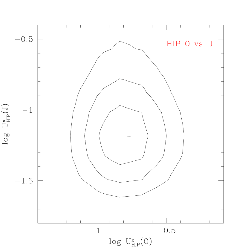
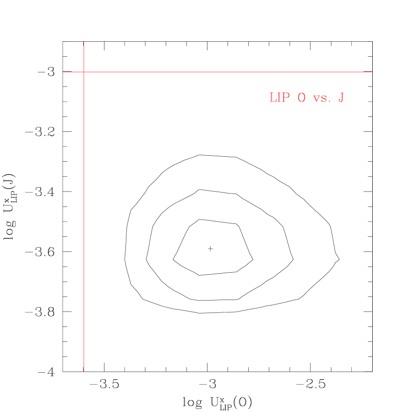
Figure 9: Confidence regions for the ionization parameter during low and high flux levels for spectra extracted from two representative flux states: j and o of the EPIC data. We calculated the contour plots for the LIP, U${}_{x}^{LIP}$(o) vs. U${}_{x}^{LIP}$(j), and for the HIP, U${}_{x}^{HIP}$(o) vs. U${}_{x}^{HIP}$(j), thus comparing the state of the gas between a high and a low flux level. The contours represent the 1, 2 and 3 $\sigma$ confidence levels. The solid lines represent the “no variation” lines for the ionization parameter [i.e. U_x(j) $=$ U_x(o)]. The plots show that the ionization parameter is not consistent with a constant value, implying opacity variations.

To further study the variations of the absorber, we have produced confidence regions of the ionization parameter during high and low flux states. Figure 9 shows these regions for spectra j and o. For the HIP, the variations are significant at a level $2\sigma$. The LIP variations are significant at a level $>3\sigma$. These tests show that changes only in the continuum cannot account for the spectral variations, further confirming that the absorbing material is responding to flux variations.

We stress again that the variations we derive for U_X are not random, but rather follow the ionizing continuum level, as expected for gas close to photoionization equilibrium. Any alternative explanation must also predict these correlations.

4.3 Photoionization Equilibrium Timescales

Since all the points for the LIP are consistent with photoionization equilibrium within 2$\sigma$ (Fig. 7b), the LIP can both recombine and ionize in a timescale shorter than the shortest time interval separating spectra with large flux changes. The largest change in flux in the shortest time is between spectra l and m (a factor of $2.1$ in flux, separated by 3 ks). Thus, we conclude that the photoionization equilibrium timescale (i.e. the time necessary for the gas to reach photoionization equilibrium with the ionizing source) $t_{eq}(LIP)<$3 ks.

For the HIP, the situation is somewhat more complicated. The spectra of the HIP at typical count-rates are all consistent with photoionization equilibrium. The extreme flux points, on the other hand, show deviations from equilibrium, i.e. they fail to respond as expected to the changes in the continuum. The three lowest count rate points (h, j, and k) each lie 2$\sigma$ above the equilibrium line for the HIP in Figure 7a (see also Fig. 1c), and so represent overionized gas, i.e. gas having $U_{X}$ larger than expected in photoionization equilibrium. Conversely, three of the four highest count rate points in Figure 7a (see also Fig. 1c, spectra c, q and u) lie $\sim$1-2$\sigma$ below the photoionization equilibrium line, and so represent underionized gas. This behavior is expected in gas close to, but not instantaneously in, equilibrium with the ionizing flux, since, depending on gas density, a cloud can respond quickly (few ks) to smooth and moderate increases/decreases of the ionizing continuum, but would require longer times to respond to fast and extreme flux changes (Nicastro et al. 1999). These delays are expected to be longer during recombination (flux decreases) than during ionization (flux increases), implying different photoionization equilibrium timescales $t_{eq}$ during different source lightcurve phases. Unlike the LIP (for which only an upper limit on $t_{eq}$ can be estimated), the behavior of the HIP allows us to set both lower and upper limits on $t_{eq}(HIP)$.

Spectra j and k correspond to a prolonged quiescent phase of the source lightcurve, following a smooth and $\sim 10$ ks long flux decrease. $U_{X}^{j}$ and $U_{X}^{k}$ are consistent with each other and each deviates from the equilibrium line by about 2$\sigma$ (Fig. 7a, the two lowest count rate points). Thus, these two spectra provide, when combined together, a robust lower limit on $t_{eq}(HIP)$. The total exposure time for spectra j, and k is $\Delta t^{j+k}\sim 10$ ks. In the following we then adopt $t_{eq}^{i,j+k}\lower 2.15277pt\hbox{$\;\buildrel>\over{\sim}\;$}10$ ks. To estimate an upper limit on $t_{eq}(HIP)$ we use spectra l and m which are separated by $\sim 3$ ks. $U_{X}^{l}$ and $U_{X}^{m}$ nearly match the increase in flux. We conclude that, for such flux variations, the photoionization equilibrium time of the HIP is $t_{eq}^{l,m}(HIP)<$3 ks.

5 The Ionized Absorber in NGC 4051: A Dense, Multi-Phase, Compact Wind

5.1 Physical conditions

In §4.3, we estimated $t_{eq}(LIP)<$3 ks (independently of the particular lightcurve phase, since the gas is always consistent with equilibrium) and $t_{eq}^{i,j+k}(HIP)\lower 2.15277pt\hbox{$\;\buildrel>\over{\sim}\;$}10$ ks (during a recombination phase where the gas does not reach equilibrium) and $t_{eq}^{l,m}(HIP)<$3 ks (during an increase in flux where the gas reaches equilibrium with the ionizing source). These response times of the gas to changes in the continuum set strong constraints on the density, $n_{e}$, and location, $R$, of the absorber relative to the continuum source.

The photoionization equilibrium timescale depends on the electron density of the absorber, during both ionization and recombination phases (Nicastro et al., 1999). Thus, we can use the above estimate of $t_{eq}$ to estimate $n_{e}$ for the LIP and the HIP. To obtain the densities, we used the approximate relation between $t_{eq}$ and $n_{e}$ derived by Nicastro et al. (1999; eq. 5) for a 3-ion atom (i.e. an atom distributed mainly among three of its contiguous ion species):

$$t_{eq}^{x{{}^{i}},x^{i+1}}\sim\left[\frac{1}{\alpha_{rec}(x^{i},T_{e})_{eq}~{}n_{e}}\right]\times\left[\frac{1}{[\alpha_{rec}(x^{i-1},T_{e})/\alpha_{rec}(x^{i},T_{e})]_{eq}+[n_{x^{i+1}}/n_{x^{i}}]}\right]$$

where “eq” indicates the equilibrium quantities, and $\alpha_{rec}(x^{i},T_{e}$) is the radiative recombination coefficient of the ion $x^{i}$, for gas with an electron temperature $T_{e}$. This is an excellent approximation for O and Ne for both the LIP (OVI-OVIII, NeVIII-NeX) and the HIP (OVII-OIX, NeIX-NeXI) because 98% of the population of these elements is concentrated in these charge states. We used recombination times from Shull & van Steenberg (1982) and the average equilibrium photoionization temperature, T${}_{LIP}\sim 3\times 10^{4}$ K and T${}_{HIP}\sim 5\times 10^{5}$ K. For the LIP, we find $n_{e}(LIP)>$8.1$\times$10⁷ cm^-3, and for the HIP $n_{e}(HIP)=(5.8-21.0)\times 10^{6}$ cm^-3 (Table 4).

The $n_{e}$ values allow us to obtain the gas pressure $P$ for each component, using the average temperature. The gas pressures of the LIP and HIP are $P_{LIP}=n_{e}(LIP)T_{LIP}>$2.4$\times$10¹² K cm^-3, and $P_{HIP}$=(2.9-10.5)$\times$10¹² K cm^-3, respectively (Table 4). The pressures of the two phases are therefore consistent with each other, suggesting that LIP and HIP may be in pressure balance, and thus two distinct phases of the same medium. This has been suggested for several other AGNs (e.g. NGC 3783, Krongold et al. 2003, Netzer et al. 2003; NGC 985, Krongold et al. 2005), but with much less tight (or no) determination of the location of the phases (thus assuming that the two phases share the same location).

5.2 Location and Structure

Given their densities, the distance $R$ of the LIP and the HIP from the central ionizing source can now be derived. We find R${}_{LIP}<$8.9 $\times$10¹⁵cm ($<$0.0029 pc, $<$ 3.5 light-days [l-d]) and R${}_{HIP}=(1.3-2.6)\times$10¹⁵ cm (0.0004-0.0008 pc, 0.5-1.0 light-days [l-d]; Table 4). Thus, not only the two gas pressures, but also the distances of LIP and HIP from the central ionizing source, are consistent with each other. This gives further support to the hypothesis that LIP and HIP are two phases of the same wind. We note that the opacity variations of NGC 4051, also reported by Ogle et al. (2004), rule out both a location of parsecs from the central source and a continuous flow in our line of sight, as suggested by these authors.

Another lower limit on $R_{HIP}$ which is less tight, but independent of the assumption that spectra i,j+k are out of photoionization equilibrium, can be obtained from the ratio $U_{x}(HIP)/U_{x}(LIP)=n_{e}(LIP)R^{2}_{LIP}/n_{e}(HIP)R^{2}_{HIP}\approx 173$. Since the LIP responds faster than the HIP to changes in the ionizing flux, then $n_{e}(LIP)>n_{e}(HIP)$. Combining these equations gives $R_{HIP}>0.076R_{LIP}$ and so $R_{HIP}>0.27$ l-d.

The observed variability of the gas also sets constraints on the structure of the ionized absorber. Assuming homogeneity in the flow, and using the column densities and number densities inferred in our analysis, the line of sight thickness and relative thickness of the wind can be estimated. The line of sight thickness is given by $\Delta R\sim N_{H}/n_{H}\simeq 1.23N_{H}/n_{e}$ (where in the last term of the equation we used $n_{e}\simeq 1.23n_{H}$ which is valid for a fully ionized gas with solar abundances). Using simple algebra we then get the relative thickness $\Delta R/R=1.23N_{H}/n_{e}R=1.23N_{H}(n_{e}R^{2})^{-1/2}(n_{e})^{-1/2}$. For our two components, we find $\Delta R_{LIP}<9\times 10^{12}$ cm, $\Delta R_{HIP}=(1.9-7.2)\times 10^{14}$ cm, and $(\Delta R/R)_{LIP}<10^{-3}$ and $(\Delta R/R)_{HIP}=(0.1-0.2)$ (Table 4).

Both the LIP and the HIP are then thin shells of gas (and hence they can be analyzed accurately in a plane-parallel configuration with respect to the central ionizing source). Moreover, $(\Delta R/R)_{LIP}\lower 2.15277pt\hbox{$\;\buildrel<\over{\sim}\;$}1\%$ $(\Delta R/R)_{HIP}$, suggesting that either the LIP is embedded in the HIP, or the LIP represents a boundary layer of the HIP. This result is consistent with our finding that the thermal pressures of the two components are consistent with each other.

5.3 Consistency Check with High Resolution Data

We stress that qualitatively similar, but quantitatively less tight conclusions on the physical state and structure of the two absorbers can be reached based on the analysis of the LS and HS high resolution RGS data only. The implied response time of the warm absorber to changes in the ionizing continuum are $t_{eq}(LIP)<$15 ks and $t_{eq}(HIP)<$15 ks (the duration of the LS observation). This implies $n_{e}(LIP)>$1.6$\times$10⁷ cm^-3, and $n_{e}(HIP)>$1.2$\times$10⁶ cm^-3; R${}_{LIP}<$2.0 $\times$10¹⁶cm and R${}_{HIP}=(1.5-5.8)\times$10¹⁵ cm ($\sim 10^{-3}$ pc). The lower limit in R_HIP comes from the ratio $U_{x}(HIP)/U_{x}(LIP)$. This confirms that the warm absorber in NGC 4051 is both dense and compact.

5.4 Comparison with Previous Observations

Using a simple time-evolving photoionization code, which included only bound-free transitions, and data with much more limited spectral resolution and S/N, Nicastro et al (1999) derived a density of $7.4\times 10^{7}$ cm^-3, and thus a distance $\sim$3 l-d for NGC4051.

Our $N_{H}$ values are factors of $\sim$20 (HIP) and $\sim$100 (LIP) smaller than the one found by Nicastro et al (1999), who measured $logN_{H}>$22.5. Our $n_{e}$ value for the HIP is also smaller by a factor 3-10. We attribute these differences to three factors, which combined independently to cause these authors to overestimate both quantities:

(1) They considered only 1 absorber to model the low-resolution ROSAT-PSPC data of NGC 4051.

(2) They estimated the absorber equivalent H column density by using a spectral model that included only bound-free transitions, neglecting the dominant contributions of resonant bound-bound absorption, particularly by Fe ions (see their Fig. 4, also Krongold et al. 2003).

(3) Consequently, they used an empirical model to measure the optical depths of the OVII and OVIII K absorption edges and find their relative abundances (i.e. the ionization parameter of the gas). The edges, however, coincide in energy with many Fe bound-bound transitions. In contrast, we fit the higher quality XMM-Newton data of NGC 4051 with two absorbing components, and use a spectral model (PHASE, Krongold et al 2003) that includes more than 3000 bound-free and bound-bound X-ray transitions from many metals (obtained mainly from the ATOMDB database, Smith et al. 2001) to derive their equivalent H column densities. As a consequence, our determination of the relative abundances of OVII and OVIII is now much more accurate than that of Nicastro et al (1999). All $N_{H}$ values determined from similar early WA models (Reynolds 1997, George et al. 1998) will likewise be strong overestimates (see Krongold et al 2003).

6 The Accretion-Disk Origin of the Ionized Wind

The sub-parsec-scale location of both absorbing components inferred independently from high resolution RGS and low resolution EPIC data can be used to test several models for the warm absorber:

(1) X-ray observations of Seyfert 2 galaxies have shown the presence of extended, pc-kpc scale, bi-cones, of ionized gas responsible for the narrow X-ray emission lines detected in the X-ray spectra of these objects (Ogle et al. 2000; Sako et al. 2000; Sambruna et al. 2001; Kinhkabwala et al. 2002; Brinkman et al. 2002; Ogle et al. 2003), and co-located, with the Narrow Emission Line Region. It has been suggested that the origin of the warm absorber is then at pc from the central source. Clearly, our results do not favor this possibility, as the origin of the wind in NGC 4051 is much further in. The narrow emission lines in Seyfert 2s should be associated with the narrow emission lines also observed in Seyfert 1s (e.g. Turner et al. 2003; Pounds et al. 2004), that do not vary in response to continuum changes in timescales of years, and thus are located much farther out than the absorber, at distances of pc, from the central source (Pounds et al. 2004 for NGC 4051). Even though our results do not support the idea that the outflow starts at pc from the ionizing source, they are consistent with the possibility that the emission lines in both Seyfert 1s and Seyfert 2s are produced by the continuation of the same wind that forms the WA, as discussed in §7.

(2) It has been suggested that the structure of the warm absorbers in our line of sight is that of a continuous range of ionization structures spanning a large radial region (of the order of pc) in the nuclear environment, and spanning more than two orders of magnitude in ionization parameter (e.g. Ogle et al. 2004, Steenbrugge et al. 2005). However, in this model, no variability is expected in the opacity of the absorber with moderate flux variations (Krongold et al. 2005b). Both the changes in ionization state of the gas following the changes of flux observed in NGC 4051, and their sub-l-d thickness, rule out a continuous radial range of ionization stages, and further support the idea of two distinct phases of a single medium for the structure of the absorber.

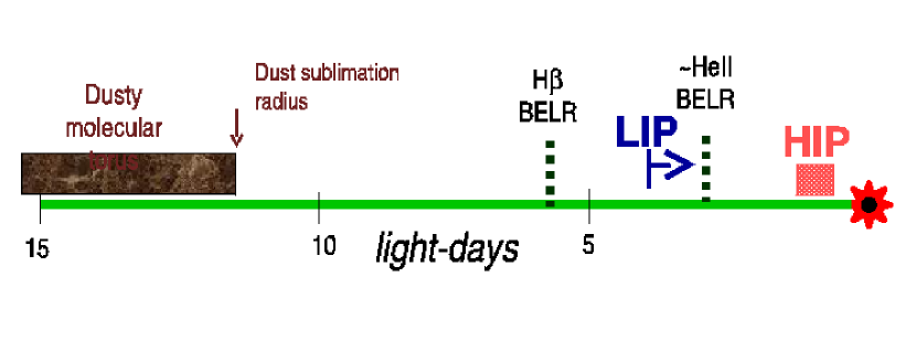
Figure 10: Location of features in the nuclear environment of NGC 4051 on a light-day scale.

(3) The remaining non-disk origin for the ionized gas – evaporation off the inner edge of the dusty obscuring torus in AGNs (Krolik & Kriss 2001) – is also ruled out for both the HIP and the LIP (and again with both high and low resolution data) in NGC 4051. The torus inner edge has to be at a distance larger or equal to the dust sublimation radius: $r_{sub}=1.3L^{1/2}_{uv,46}T^{-2.8}_{1500}$ pc. Here $L_{uv,46}$ is the UV luminosity of the source in units of $10^{46}$ erg s^-1 cm^-2 and $T_{1500}$ is the grain evaporation temperature in units of 1500 K (Barvainis 1987). For NGC 4051 log$L(1450A)=26.38\pm 0.05$ erg s^-1 Hz^-1 (Constantin & Shields 2003) and, assuming a dust temperature of 1500 K, we obtain $r_{sub}(NGC4051)$= 3$\times$10¹⁶cm (0.01 pc, 12 l-d). This distance is a factor of 3.4 and 12 larger, respectively, than the LIP and HIP upper limits. A hotter assumed dust temperature does not remove the discrepancy between the HIP and LIP location and the inner edge of the obscuring torus as even for dust at a maximal temperature of 2000 K, $r_{sub}$ is only reduced by a factor 0.45. Moreover, this brings the sublimation radius to the same distance as the H$\beta$ BELR in NGC 4051, even though the torus must be located outside the BELR for unification models to work. Changing the UV luminosity also does not help if the X-ray luminosity changes in parallel, as $r_{sub}$ and $R_{HIP}$ both scale as $L^{0.5}$. Finally, this estimate of $r_{sub}$ is only a lower limit for a putative torus-wind in NGC 4051. As Krolik & Kriss (2001) pointed out, the innermost edge of a molecular torus, at which an ionized wind producing the absorption seen in the X-rays can form, is not simply at the sublimation radius. This edge must be derived using photoionization arguments for the observed gas, given the density of a putative torus wind (which is at least 2 order of magnitudes lower than the densities we estimate here for the LIP and the HIP). Following these arguments, Blustin et al. (2005) derive a distance for the inner edge of the torus, of $r_{torus}\simeq 0.15$ pc for NGC 4051. This is 52 and 178 times larger than our upper limits on the LIP and HIP distances from the central ionizing source, respectively. Figure 10 gives a schematic linear scale diagram of the distance in light-days of the different AGN components to the central source.

Having ruled out all large-scale locations for the ionized wind, we can look more carefully at the possible small-scale locations. The size of the H$\beta$ BELR in NGC 4051, from reverberation mapping is 5.9 l-d (Peterson et al. 2000). As $R_{HIP}=$0.5-1.0 lt-days, the HIP is clearly much smaller than the H$\beta$ BELR. The LIP location, on the other hand, is marginally consistent with the H$\beta$ BELR. The higher ionization HeII broad emission line has a smaller measured reverberation lag $\;\buildrel<\over{\sim}\;$1 l-d (Peterson et al. 2000), consistent with the HIP location. This broad line has a wing blueshifted by $\sim$400 km s^-1 compared to H$\beta$, suggesting a wind component, which in turn suggests a connection with the X-ray warm absorber (which has outflow velocities of 600-2340 km s^-1, e.g. Collinge et al. 2001). Peterson et al. (2000) measure FWHM(HeII)= 5430 km s^-1 (in the rms spectrum). If the HeII gas were virialized, the HeII BELR is $\sim$2 times closer in than the H$\beta$ BELR, i.e. $\sim$2.5 l-d, which is consistent with the largest allowed LIP size. The HeII outflow, however, implies a somewhat narrower virial component to the line and so a larger distance from the black hole. An accurate measurement of the HeII reverberation lag would give a definitive answer.

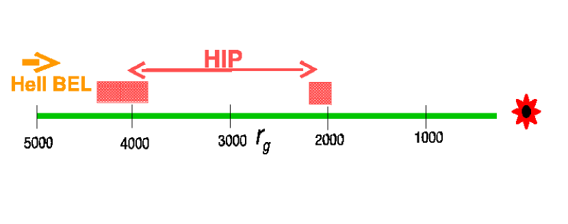
Figure 11: Location of features in the nuclear environment of NGC 4051 on a gravitational radius scale.

The location of the HIP in Schwarzschild radii ($R_{s}$) implies that the origin of the HIP is related to the accretion disk. In these units, $R_{HIP}$= 2300 - 4600 $R_{s}$, which locates the outflow in the outer regions of the accretion disk, but at distances shorter than the radius where an $\alpha$-disk becomes gravitationally unstable ($\sim 35000~{}$R_s; Goodman 2003). The LIP is also likely related to the disk, as $R_{LIP}<15800R_{s}$. Figure 11 gives a scale diagram of the location of the different AGN components. We note that NGC 4051 has a fairly low accretion rate relative to Eddington value (10%, Peterson et al. 2004) for a Narrow Line Seyfert 1 Galaxy (Pounds et al. 1995). This could be because we are seeing it in a pole-on configuration and so this gives narrower broad emission lines than normal. If so then the black hole mass for this object is underestimated, and the location of the absorbing components in $R_{s}$ should decrease, making a more compact absorber.

7 Geometry of the Wind

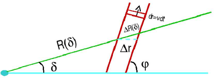
Figure 12: Disk-Wind in a conical geometry. $\phi$ is the angle formed by the wind and the disk and $\delta$ the angle between the disk and the observer’s line of sight. $R$ is the distance from the continuum source to the wind and $\Delta~{}R$ its thickness.

Our findings considered alone, are consistent with thin spherical shells of material which are expelled radially from the central ionizing source. However, we consider this configuration implausible because of the fine tuning required in the frequency with which these shells of material would have to be produced to explain the high occurrence of WAs in AGNs, and yet still avoid having the thin shells degenerate into a continuous flow (which is strictly ruled out for NGC 4051). The next simplest geometrical configuration is that of a bi-conical wind (Fig. 12, Elvis 2000). All our estimates for the physical and geometrical quantities of the two X-ray absorbers of NGC 4051 are consistent with this scenario, and recent magneto-hydrodynamical simulations also favor this interpretation (Everett 2005).

We note that assuming this bi-conical geometry, our results are consistent with the possibility that the extended, pc-kpc scale, emitting bi-cones observed in Seyfert 2s are part of the same flow that forms the WA (e.g. NGC 1068, Crenshaw & Kraemer 2000). In this case the NELR and X-ray emitting gas would be the continuation of the WA wind but at large radii. A constant ionization parameter with radius could be expected if the density decreases with the inverse square of the distance, as observed by Bianchi et al. (2006) for the kpc scale nebulae in type 2 objects.

The possible connection between these two components requires that the emitting bi-cones are not filled with material (as otherwise, from a pole-on line of sight we should observe an absorber forming a continuous radial range of ionization stages, which is already ruled out). Then from a pole-on configuration no absorption would be observed, as no material would cross our line of sight (Fig. 12) in agreement with the detection rate of WA. The absorber would be observed as a transverse flow (which is required by observations, see below), through the inner and outer edges of the bi-cone, and close to the base of the flow, as shown in Figure 12. The observed X-ray emission would be produced by the same bi-conic flow, but at much larger distances. In this scenario absorption and emission are then part of the same wind, although the two measured distances are very different. This idea agrees with recent results on Seyfert 2 galaxy NGC 1068 by Das et al. (2006), who found that the best kinematic model for the X-ray bi-conical emission requires empty cones, with a geometry consistent to the one found here for the warm absorber.

8 Wind Mass and Kinetic Energy Outflow Rate

With the location and density of the X-ray absorbing material in hand, and assuming the above bi-conical geometry, we can now estimate the mass outflow rate of the wind.

The escape velocity ($v_{esc}$) from the location of the HIP is $\sim$4000-6000 km s^-1, which is 10 times larger than the measured outflow velocities in our line of sight for the X-ray warm absorber in NGC 4051 (v${}_{r}\sim$ 500 km s^-1). The true outflow velocity is most likely to be 2 times larger (i.e. for a 60 degree angle between our line of sight and the wind). This, however is still $\sim$5 times smaller than the escape velocity at the distance of the HIP. Either the wind falls back, or the wind is accelerated after it crosses our line of sight. If the gas were falling back, evidence of inflowing material in absorption should be detected (in the X-ray band or in the UV band through the Ly$-\alpha$ line if the gas has cooled down), and redshifted absorbing systems are rare and do not necessarily imply inflow (e.g. Vestergaard 2003). Since there is evidence of a transverse wind across our line of sight in other AGNs (Mathur et al. 1995; Crenshaw, Kraemer & George 2003) which is accelerating (Arav 2004), the latter option is preferable. In addition, radiatively line driven wind models (Proga & Kallman 2004) and phenomenological derived models (Elvis 2000), require later acceleration of the wind. Furthermore, in a conical wind, the material of the warm absorber must be rotating with Keplerian velocity ($v_{Kep}$) around the center (at least at the base of the wind). Since the escape velocity scales with $v_{Kep}$ as $v_{esc}=\sqrt{2}~{}v_{Kep}$, the wind already has half the kinetic energy needed to escape. All these point to an escape of the material from the central regions.

In a bi-conical wind, from a direction looking directly along the cone opening angle an observer would see a much larger column density, $>1.5\times 10^{23}$ cm^-2 (assuming the wind can reach $v_{esc}$) mostly due to the LIP (see Appendix A.1). This high N_H flow would also be seen to have a larger velocity, perhaps much larger, as in WA we may be seeing the flows before they get fully accelerated. Thus, from this special direction the NGC 4051 wind would begin to resemble a ‘Broad Absorption Line’ (BAL) system (Elvis 2000).

To evaluate the mass loss rate in the WA wind let $\delta$ be the angle between our line of sight to the central source and the accretion disk plane, and $\phi$ be the angle formed by the wind with the accretion disk (see Fig. 12). We can then derive a formula for the mass outflow rate and write it in terms of the observables $v_{r}$ (the line of sight outflow velocity), N_H (the line of sight equivalent H column density), and $R$ (see Appendix A.2 for full details on the derivation of this formula):

$$\dot{M}_{w}=0.8\pi m_{p}N_{H}v_{r}Rf(\delta,\phi)$$

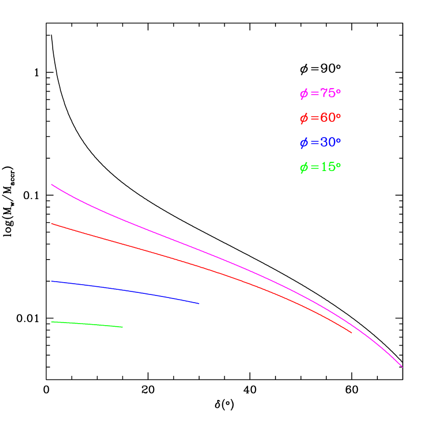
Figure 13: Mass outflow rate (in accreted mass units) vs. line of sight angle ($\delta$) for several values of the inclination of the wind ($\phi$). For reasonable angles the mass outflow only changes by a factor $\sim 2$.

where $f(\delta,\phi)$ is a factor that depends on the particular orientation of the disk and the wind, and for all reasonable angles ($\delta>20^{o}$ and $\phi>45^{o}$) is of the order of unity (with a variation by a factor of 2, see Fig. 13). Thus, for a vertical disk wind ($\phi=\pi/2$) and an average Seyfert 1-like line of sight angle $\delta=30^{0}$ $f(\delta,\phi)$=1.5 (see A.2), and we find: $\dot{M}_{w}(HIP)=(0.7-1.4)\times 10^{-4}$ M_⊙ yr^-1 and $\dot{M}_{w}(LIP)<0.9\times 10^{-4}$ M_⊙ yr^-1. For NGC 4051, assuming 10% accretion efficiency, the observed accretion rate is $\dot{M}_{accr}=4.7\times 10^{-3}$ M_⊙ yr^-1 (Peterson et al. 2004), so $\dot{M}_{w}(HIP)=(0.02-0.03)\dot{M}_{accr}$ and $\dot{M}_{w}(LIP)<0.02$ $\dot{M}_{accr}$. Therefore, the total mass outflow rate from the LIP and the HIP, in NGC 4051, is $\dot{M}_{out}=(0.02-0.05)\dot{M}_{accr}$. Thus, the total mass outflow rate is only a small fraction of the observed accretion rate. We stress here that these estimates of the mass outflow rate from the X-ray disk winds of NGC 4051 depend only weakly on the assumed geometrical configuration (unless NGC 4051 is seen close to pole-on, see end of §6). Their robustness is due to the strong constraints that we can independently set on the physical properties of the absorbers.

9 Possible Implications for Galaxy Evolution and Cosmic Feedback

Given the importance that recent theoretical studies have bestowed on AGN winds (see below), it is worth investigating the potential implications that warm absorber winds can have on their large scale environment. Some aspects of this discussion are speculative and we do not pretend to present a physical model. Rather, we present only an analysis in terms of energy budgets and order of magnitude estimates.

Assuming that the black hole mass of NGC 4051 was all accreted (M${}_{BH}=1.9\times 10^{6}$ M_⊙, Peterson et al. 2004), we can calculate the integrated lifetime mass lost due to the X-ray winds, M${}_{out}=(0.4-1.0)\times 10^{5}$ $M_{\odot}$ (M${}_{out}=0.02-0.05\times$ M_BH). This number is too small for the winds to have an important influence on the ISM or IGM. However, NGC 4051 is on the low end of AGN black hole masses, luminosities ($L_{bol}=2.5\times 10^{43}$ ergs s^-1, Ogle et al. 2004) and accretion rates relative to Eddington value (10%, Peterson et al. 2004). If the measured ratio $\dot{M}_{out}/\dot{M}_{accr}$ of NGC 4051 is representative of the quasar population, then for winds in powerful quasars ($L_{bol}\sim 10^{47}$ ergs s^-1, M${}_{BH}=$ few$\times 10^{9}$ M_⊙) the total mass outflow could be as large as $M_{out}\sim$ few$\times 10^{8}$ M_⊙ (neglecting any additional mass from the interstellar medium entrained in the wind). This mass is comparable to that available from the most optimistic estimates of powerful ULIRGs’ winds (which include significant mass entrainment, e.g. Veilleux et al. 2005) and could, in principle, be deployed into the IGM surrounding the quasar’s host galaxy.

The quasar nuclear environment is unusually rich in metals, with metallicities several times solar found in winds from local AGN. Fields et al. (2005) found metallicities 5 times solar in Mrk 1044, and higher values are likely for high z, high luminosity quasars (e.g. Hamman & Ferland 1999). On the other hand, metallicities in Lyman $\alpha$ forest at $z\sim 3$ are low (0.01-0.001 times solar, Pettini 2004). So, assuming that quasar winds can escape the host galaxy, they could feed their local IGM with highly metal enriched material. This would create local inhomogeneities in the metal content of the IGM around such quasars. From our line of sight to powerful quasars, the measured column density of metals in IGM systems close to the central object (at distances up to a few hundred kpc) would then be much larger ($>$100) than in Lyman $\alpha$ systems located far away from quasars. Thus, metal rich IGM systems may be significantly stronger close to powerful quasars.

Simulations show that, if quasar winds are to be the main process controlling the evolution of the host galaxy and the surrounding IGM, they require output kinetic energies of the order of $\sim 10^{60}$ erg (e.g. Hopkins et al. 2005; Scannapieco 2004; King 2003). Such energy outputs would be enough to produce the well known relation between the central black hole mass and bulge velocity dispersion (Ferrarese & Merrit 2000; Gebhardt et al. 2000), or to heat the IGM controlling structure formation.

However, lower wind energy outputs may still have an important effect on their environments. For instance, unbinding the hot phase of the ISM may be enough to stop large scale star formation processes in a host galaxy. As this confining medium escapes from the galaxy, the warm and cold phases must expand, decreasing their temperature and density, and producing a fast decline in the star formation rate (a full analysis will be presented in a forthcoming paper, see also Natarajan et al. 2006). Evaporating the hot-ISM from a typical galaxy requires that the wind heats this medium from its current temperature of $\sim 10^{6}$ K to $\sim 10^{7}$ K. The energy needed to increase the gas temperature by this amount is E$\sim$N${}_{TOT}k$T (where N_TOT is the total number of particles in the disk and T$\sim 10^{7}$ K). Assuming a galactic disk of radius 10 kpc and thickness 0.1 kpc, with a hot-ISM electron density of $10^{-2}$ cm^-3 (Smith et al. 2006), implies that an energy input of $\sim 10^{55}$ erg into the hot-ISM would heat it to T$\sim 10^{7}$ K and would produce this medium to evaporate, ceasing star formation. For the observed velocities found in WAs ($\sim$ 500 km s^-1), in $10^{7}$ yr the gas would move 5 kpc away from the central region, into the host galaxy. This time is consistent with the lifetime inferred for quasars ($10^{7}$-$10^{8}$ yr), and suggests that the wind could indeed affect the host galaxy. The total kinetic power released by the wind in NGC 4051 (given by $\dot{M}_{out}v^{2}/2$) is $\sim 10^{38}$ erg s^-1 (assuming the observed outflow velocity of 500 km s^-1), and the total kinetic energy deployed into the ISM/IGM surrounding NGC 4051 would be only $\sim 10^{54}$ erg. This energy is still an order of magnitude smaller than the $10^{55}$ erg required to disrupt the hot phase of the ISM. However, even WA winds in typical Seyfert 1 galaxies (with black hole masses few$\times 10^{7}$ M_⊙) would reach this energy, and could have an effect on the hot-ISM and star formation processes of their hosts.

If the measured ratio $\dot{M}_{out}/\dot{M}_{accr}$ is representative of quasars, then (assuming velocities in our line of sight of 500 km s^-1) the total energy deployed by a powerful quasar into the host galaxy ISM or the IGM, during the AGN active phase, could be $\sim$ $few\times 10^{57}$ erg. Thus, winds in powerful quasars could have important effects controling star formation in their hosts (disrupting the hot-ISM), but would still be too weak to have a drastic influence on the whole galaxy evolution. We suggested, however, that we are not seeing the full terminal velocity of the wind (§8; Proga & Kallman 2004; Elvis 2000). Then, if the winds are accelerated to v$\sim$5000 km s^-1, i.e. by a factor of 10 (which is the ratio between the velocities found in WAs and BALQSOs), the total kinetic energy deployed by these systems could reach $\sim$ few$\times 10^{59}$ erg, similar to the binding energy of massive galactic bulges. This energy is comparable to the 10⁶⁰ erg required by simulations for quasar winds to be critically important in feedback processes (e.g. Hopkins et al. 2005; Scannapieco 2004; King 2003).

Thus, despite our low mass loss rate estimates, it still remains possible that AGN winds are important for at least two major feedback mechanisms: (1) the evolution of their host galaxies, putting energy into the ISM of the host and controlling the accretion process, thus regulating the black hole growth (the relationship between the mass of the central black hole in galaxies and the velocity dispersion of the galactic bulge), and/or (2) enriching with metals the IGM and heating this medium, controlling the accretion of material onto galaxies (thus controlling structure formation). Furthermore, the above conclusions are based on a one-object analysis. The ratio $\dot{M}_{out}/\dot{M}_{accr}$ could well be larger for quasars, increasing the mass and energy output of quasar winds. To fully determine what role do AGN winds play require measuring AGN geometry and kinematics for more normal objects, preferably over a range of black hole masses and Eddington ratios.

10 Conclusions

The response of the ionization state of the absorbing gas in NGC 4051 to variations in the ionizing continuum immediately rules out a radially continuous flow and a large scale (kpc) origin for the WA (at the location of the NLR). With a detailed analysis we were able to constrain the density and location of the absorbing gas. The two-component absorber in NGC 4051 is dense [$n_{e}=(5.8-21.0)\times 10^{6}$ cm ^-3 for the high ionization absorber and $n_{e}>$8.1$\times$10⁷ cm^-3 for the low ionization one], and its location is close to the continuum source, at distances 0.5-1.0 l-d (2200 - 4400R_s) and $<$ 3.5 l-d ($<~{}15800$R_s) for the high and low ionization components, respectively. The two absorbing components are in pressure balance strongly suggesting a two-phase medium. These results for NGC 4051 place this WA wind on an accretion disk scale, well within the inner edge of a dusty torus or the low ionization H$\beta$ broad emission line region. A continuous radial wind with varying ionization state is doubly ruled out, as the absorbers have a thickness $\Delta$R $<<$ R. This thinness also makes purely radial motion unlikely, given the 50% incidence of ionized absorbers in AGNs. A bi-conical outflow largely transverse to our line-of-sight is the simplest geometry that can produce the small relative thickness of the absorbers and their high covering factor. Since the smallest radius found is the one that gives the strongest constraint on the origination radius of WAs, we conclude that AGN winds must arise from the accretion disk and points us toward physical models for the production of winds from AGN disks.

An accretion disk wind can tie together all the absorption and emission features in the spectra of AGN, including the broad emission lines (Elvis 2000). The location of the He II BELR is consistent with the position of the absorber, supporting the above picture. Our results are also consistent with the idea that the pc, bi-conical, emission regions observed in Seyfert 2 galaxies are the continuation, at much larger distances from the central region, of the warm absorber winds.

The implied mass outflow rate of the warm absorber wind in NGC 4051 is a small fraction of the mass accretion rate ($\dot{M}_{out}$ = 2-5% $\dot{M}_{accr}$). If all the mass in the central black hole of NGC 4051 was accreted, then the total outflow of mass produced by the wind would be M${}_{out}=(0.4-1.0)\times 10^{5}$ $M_{\odot}$ and the total kinetic energy released by the flow would be $\sim 10^{54}$ erg. This energy is too small to unbind the entire ISM of the host galaxy in this AGN, but is comparable to the energy required to disrupt the hot phase of the ISM, which could then disrupt star formation. This suggests that even mild winds in Seyfert galaxies might have an important effect in their host galaxies.

Only through fully understanding AGN outflows, we will be able to calculate AGN feedback accurately. Further studies of less extreme AGNs over a large range of black hole masses and accretion rates relative to Eddington will give a definitive answer.

Appendix A Appendix

A.1 The Column Density of a Disk-Wind observed directly down the cone

In this section we derive the column density of a conical wind viewed down the cone. We assume that the cone bends forming a funnel-shaped geometry. In such geometry, after the point when the flow bends, it can be considered again as a radial flow. From the equation of mass conservation it follows that

$$n_{H}(R)=n_{oH}\times(v(R)/v_{o})^{-1}\times(R/R_{o})^{-2}$$ ()

where the subscript $o$ stands for the conditions at the base of the radial flow, i.e. the bending point of the flow in the funnel-shape geometry. We assume that the properties at the base of the radial flow are equal to the measured properties in our analysis.

Now consider two forces acting on the gas: the gravitational attraction of the central black hole, and the radiative force on the warm absorber. Since both forces are proportional to $R^{-2}$, we can simply write the equation of motion for the warm absorber as:

$$M_{out}\frac{dv(R)}{dt}=\frac{k}{R^{2}}$$ ()

with $k$ constant. It can be easily shown that for an object with luminosity L$\sim$0.05 L_E radiative force will dominate over gravitacional force. Thus for most Seyfert 1 galaxies and quasars $k>$0. Solving equation (2) for $V(R)$ gives

$$\frac{v(R)}{v_{o}}=\left[1+\frac{2k}{v_{o}^{2}R_{o}M_{out}}\left(1-\left[\frac{R}{R_{o}}\right]^{-1}\right)\right]^{\frac{1}{2}}$$ ()

From the equation of energy conservation for the flow

$$\frac{1}{2}M_{out}v_{\infty}^{2}=\frac{1}{2}M_{out}v_{o}^{2}+\frac{k}{R_{o}}$$ ()

where the subscript $\infty$ stands for the final velocity of the wind. It can be immediately derived that

$$\frac{2k}{v_{o}^{2}R_{o}M_{out}}=\left(\frac{v_{\infty}}{v_{o}}\right)^{2}-1$$ ()

Replacing equation (5) in (3) gives

$$\frac{v(R)}{v_{o}}=\left[1+\left(\left(\frac{v_{\infty}}{v_{o}}\right)^{2}-1\right)\left(1-\left[\frac{R}{R_{o}}\right]^{-1}\right)\right]^{\frac{1}{2}}$$ ()

Replacing equation (6) into equation (1) and integrating for the column density $N_{H}=\int n_{(}r)dr$ (where the integral runs from $R_{o}$ to $\infty$) it is found that

$$N_{\infty}=\frac{n_{o}R_{o}}{1+(v_{\infty}/v_{o})}$$ ()

Thus the column density only depends on the values at the base of the radial flow.

We assume that the conditions measured for the LIP and the HIP in NGC 4051 are representative of the conditions at the base of the radial flow. Thus we assume that $n_{o}(H)$ is equal to the value obtained in our analysis, that $v_{o}$ is equal to the observed line of sight velocity of the flow and that $v_{\infty}=v_{esc}$. With this conditions, and assuming $(v_{esc}/v_{o})\sim 10$ (if the flow viewed directly down is observed as a BALQSO) then $N_{H}(LIP)>1.5\times 10^{23}$ cm^-2 and $N_{H}(HIP)\sim 4\times 10^{21}$ cm^-2. So, the column density in this case is dominated by the LIP, and the total equivalent H column density measured down the flow should be $N_{H}(LIP)>1.5\times 10^{23}$ cm^-2.

A.2 The Mass Outflow Rate of a Disk-Wind in a conical Geometry

Let $\delta$ be the angle between our line of sight to the central source and the accretion disk, and $\phi$ the angle formed by the wind with the accretion disk, as shown in Figure 12. If $r$ and $\Delta r$ are the projections of the line of sight distance of the wind from the central source ($R(\delta)$) and the line of sight effective thickness of the wind ($\Delta R(\delta)=1.23N_{H}/n_{e}$) onto the accretion disk plane, then $r=Rcos\delta$ and $\Delta r=\Delta Rcos\delta$. Let us further suppose that the true thickness $\Delta R=\Delta rsin\phi$ of the wind (between the two conical surfaces) stays constant with $\delta$ (i.e. $\Delta r\neq\Delta r(\delta)$). With these relations we can now estimate the net mass loss rate in the outflow. In general, $\dot{M}_{w}=(1/1.23)n_{e}m_{p}\times v_{r}/sin(\phi-\delta)\times A$, where, $v_{r}$ is the line of sight component of the outflow velocity and $A$ is the area (constant with $\delta$) effectively filled by the gas and defined by the projection of the section of two concentric cylinders perpendicular to the accretion disk plane, with inner and outer radii $r$ and $r+\Delta r$, onto the plane perpendicular to the outflow velocity: $A=\pi[(r+\Delta r)^{2}-r^{2}]sin\phi$. Rearranging this expression in terms of observables, $\dot{M}_{w}=0.8n_{e}m_{p}\times v_{r}/sin(\phi-\delta)\times\pi[(R+\Delta R)^{2}-R^{2}]cos^{2}\delta sin\phi=0.8(n_{e}R^{2})m_{p}[v_{r}/sin(\phi-\delta)]\times\pi[(\Delta R/R)^{2}+2(\Delta R/R)]cos^{2}\delta sin\phi$. This formula can be simplified to $\dot{M}_{w}=0.8\pi m_{p}N_{H}v_{r}Rf(\delta,\phi)$ (where $f(\delta,\phi)$ collects the angle dependences), since $(\Delta R/R)^{2}$ is negligible due to the small relative thickness of the absorbers.

Thus, for a vertical disk wind ($\phi=\pi/2$) and an average Seyfert 1-like line of sight angle $\delta=30^{0}$ we find: $\dot{M}_{w}(HIP)=(0.7-1.4)\times 10^{-4}$ M_⊙ yr^-1 and $\dot{M}_{w}(LIP)<0.9\times 10^{-4}$ M_⊙ yr^-1. For NGC 4051 $L_{BOL}\sim 2.7\times 10^{43}$ erg s^-1 (Ogle et al. 2004). Assuming 10% accretion efficiency the observed accretion rate for NGC 4051 is $\dot{M}_{accr}=4.7\times 10^{-3}$ M_⊙ yr^-1. Thus the mass outflow rates, in terms of mass accretion, are $\dot{M}_{w}(HIP)=(0.02-0.03)\dot{M}_{accr}$ and $\dot{M}_{w}(LIP)<0.02$ $\dot{M}_{accr}$. This outflow rates cannot change much (factors $\sim 2$) for different (reasonable) choices of $\delta$ and $\phi$ ($\delta>20^{o}$ and $\phi>45^{o}$), as can be seen from Figure 16.

Table 1: Narrow Emission Lines used in the models.

Line	$\lambda_{source}$	Width (km s-1)	Flux (10-5 erg cm-2 s-1)
C VI Lyα	33.79$\pm$0.03	358$\pm$89	5.5$\pm$1.5
N VI 1s-2p (f)	29.59$\pm$0.03	137$\pm$31	2.5$\pm$1.0
O VII 1s-2p (f)	22.14$\pm$0.03	194$\pm$37	12.0$\pm$2.5
O VII 1s-2p (i)	21.84$\pm$0.03	194$\pm$37a	5.5$\pm$1.5
O VII 1s-2p (r)	21.65$\pm$0.06	194$\pm$37a	3.0$\pm$1.5
O VIII Lyα	19.01$\pm$0.02	134$\pm$21	6.5$\pm$1.0
Fe XVII 2p-3s	17.10$\pm$0.02	397$\pm$93	2.5$\pm$1.0
Ne IX 1s-2p (f)	13.73$\pm$0.02	98$\pm$21	3.0$\pm$1.0

Table 2: Best-fit values over spectra extracted for the whole, time integrated, XMM-Newton RGS and EPIC observation.

RGS	$\Gamma$	BB1(kT) (keV)	BB2(KT) (keV)	log(NH) [cm-2]	log(Ux)	vel. (km s-1)
HIP	1.74$\pm 0.5$	0.137$\pm{.06}$	0.064$\pm{.08}^{a}$	21.42$\pm{.12}$	-0.76$\pm{.08}$	537$\pm{130}$
LIP	1.74$\pm 0.5$	0.137$\pm{.06}$	0.064$\pm{.08}^{a}$	20.73$\pm{.17}$	-2.90$\pm{.10}$	492$\pm{97}$
EPIC	$\Gamma$	BB1(kT) (keV)	BB2(KT) (keV)	log(NH) [cm-2]	log(Ux)	vel. (km s-1)
HIP	1.97$\pm 0.09$	0.141$\pm{.03}$	0.064$\pm{.08}$	21.42$\pm{.12}$b	-0.72$\pm{.08}$	537$\pm{130}$b
LIP	1.97$\pm 0.09$	0.141$\pm{.03}$	0.064$\pm{.08}$	20.73$\pm{.17}$b	-2.97$\pm{.14}$	492$\pm{97}$b

Table 3: RGS and EPIC-PN models for the HS and the LS.

Abs.	RGS (HS)	RGS (LS)
HIP log(Ux)	$-0.72_{-.05}^{+.08}$	$-1.31_{-.25}^{+0.38}$
LIP log(Ux)	$-2.91_{-.11}^{+.10}$	$-3.65_{-.50}^{+.25}$
Abs.	EPIC (HS)	EPIC (LS)
HIP log(Ux)	$-0.68_{-.04}^{+.09}$	$-1.24_{-.11}^{+.16}$
LIP log(Ux)	$-2.98_{-.10}^{+.15}$	$-3.72_{-.17}^{+.17}$

Table 4: Physical parameters of High and Low Ionization Absorbers

Abs.	NH	Te	$(n_{e}R^{2})$	$n_{e}$	Pe	$R$	$\Delta R$	$(\Delta R/R)$
	$10^{21}$ cm-2	$10^{5}$ K	$10^{38}$ cm-1	$10^{7}$ cm-3	$10^{12}$ K cm-3	$10^{15}$ cm	$10^{14}$ cm
HIP	$(3.2\pm{2.2})$	$(5.4\pm{1.4})$	$(0.38\pm 0.05)$	(0.58-2.1)	(2.9-10.5)	(1.3-2.6)	(1.9-7.2)	(0.1-0.2)
LIP	$(0.59\pm{0.28})$	$(0.28\pm{.04})$	$(66\pm 3)$	$>8.1$	$>2.4$	$<8.9$	$<0.09$	$<10^{-3}$

Figure 8: Confidence regions for the thermal component normalization (kT=.14 keV) vs. the ionization parameter for the HIP and the LIP. The contours represent the 1, 2 and 3 $\sigma$ confidence levels. The spectra corresponds to time region o. There is no correlation between these parameters, showing that the continuum parameters for the blackbody do not influence the measured correlation U_x vs. flux. Similar results are found for the other 20 time regions. The normalization is in L₃₉/(D₁₀)² units, where L₃₉ is the source luminosity in units of 10³⁹ erg s^-1 and D₁₀ is our distance to the source in units of 10 kpc.

References

- Arav (2004) Arav, N. 2004, ASP Conf. Ser. 311: AGN Physics with the Sloan Digital Sky Survey, 311, 213
- (2) Barvainis R., 1987 ApJ 320, 537
- (3) Behar, E., Rasmussen, A. P., Blustin, A. J., Sako, M., Kahn, S. M., Kaastra, J. S., Branduardi-Raymont, G., & Steenbrugge, K. C. 2003, ApJ, 598, 232
- (4) Blustin, A. J., Page, M. J., Fuerst, S. V., Branduardi-Raymont, G., & Ashton, C. E. 2005, A&A, 431, 111
- Brinkman et al. (2002) Brinkman, A. C., Kaastra, J. S., van der Meer, R. L. J., Kinkhabwala, A., Behar, E., Kahn, S. M., Paerels, F. B. S., & Sako, M. 2002, A&A, 396, 761
- Ciotti & Ostriker (1997) Ciotti, L., & Ostriker, J. P. 1997, ApJ, 487, L105
- (7) Collinge, M. J. et al. 2001, ApJ, 557, 2
- (8) Constantin A. & Shields J.C., 2003, PASP, 115, 592.
- Costantini et al. (2006) Costantini, E., et al. 2006, ArXiv Astrophysics e-prints, arXiv:astro-ph/0609385
- (10) Crenshaw, D. M., Kraemer, S. B., & George, I. M. 2003, A&A Rev., 41, 117
- Das et al. (2006) Das, V., Crenshaw, D. M., Kraemer, S. B., & Deo, R. P. 2006, AJ, 132, 620
- (12) Elvis, M., Wilkes, B. J., & Lockman, F. J. 1989, AJ, 97, 777
- (13) Elvis, M. 2000, ApJ, 545, 63
- Elvis et al. (2002) Elvis, M., Marengo, M., & Karovska, M. 2002, ApJ, 567, L107
- Everett (2005) Everett, J. E. 2005, ApJ, 631, 689
- Ferrarese & Merritt (2000) Ferrarese, L., & Merritt, D. 2000, ApJ, 539, L9
- (17) Fields, D. L., Mathur, S., Pogge, R. W., Nicastro, F., Komossa, S., & Krongold, Y. 2005, ApJ, 634, 928
- Gabel et al. (2005) Gabel, J. R., et al. 2005, ApJ, 631, 741
- Gabel et al. (2003) Gabel, J. R., et al. 2003, ApJ, 595, 120
- Gebhardt et al. (2000) Gebhardt, K., et al. 2000, ApJ, 539, L13
- George et al. (1998) George, I. M., Turner, T. J., Netzer, H., Nandra, K., Mushotzky, R. F., & Yaqoob, T. 1998, ApJS, 114, 73
- (22) Goodman J., 2003, MNRAS, 339, 937
- (23) Grevesse, M. N., Noels A., & Sauval, A. J. 1993, A&A, 271, 587
- Hamann & Ferland (1999) Hamann, F., & Ferland, G. 1999, ARA&A, 37, 487
- Hopkins et al. (2005) Hopkins, P. F., Hernquist, L., Cox, T. J., Di Matteo, T., Robertson, B., & Springel, V. 2005, ApJS preprint doi:10.1086/’499298
- Kaastra et al. (2004) Kaastra, J. S., et al. 2004, A&A, 428, 57
- (27) King, A. 2003, ApJ, 596, L27
- Kinkhabwala et al. (2002) Kinkhabwala, A., et al. 2002, ApJ, 575, 732
- (29) Krolik, J. H. & Kriss, G. A. 2001, ApJ, 561, 684
- Krolik & Kriss (1995) Krolik, J. H., & Kriss, G. A. 1995, ApJ, 447, 512
- (31) Krongold, Y., Nicastro, F., Brickhouse, N.S., Elvis, M., Liedahl D.A. & Mathur, S. 2003, ApJ, 597, 832 (K03)
- (32) Krongold, Y., Nicastro, F., Elvis, M., Brickhouse, N. S., Mathur, S., & Zezas, A. 2005, ApJ, 620, 165
- (33) Krongold, Y., Nicastro, F., Brickhouse, N. S., Elvis, M., & Mathur, S. 2005b, ApJ, 622, 842
- Magorrian et al. (1998) Magorrian J. et al. 1998, AJ, 115, 2285
- (35) Mathur, S., Elvis, M., & Wilkes, B. 1995, ApJ, 452, 230
- (36) McHardy, I. M., Papadakis, I. E., Uttley, P., Page, M. J., & Mason, K. O. 2004, MNRAS, 348, 783
- (37) Natarajan et al. 2006., submitted
- (38) Netzer H., 1996, ApJ, 473, 781
- Netzer et al. (2002) Netzer, H., Chelouche, D., George, I. M., Turner, T. J., Crenshaw, D. M., Kraemer, S. B., & Nandra, K. 2002, ApJ, 571, 256
- Netzer et al. (2003) Netzer, H., et al. 2003, ApJ, 599, 933
- (41) Nicastro, F., Fiore, F., & Matt, G. 1999, ApJ, 517, 108
- Nicastro et al. (2005) Nicastro, F., et al. 2005, ApJ, 629, 700
- Nulsen et al. (2005) Nulsen, P. E. J., McNamara, B. R., Wise, M. W., & David, L. P. 2005, ApJ, 628, 629
- Ogle et al. (2000) Ogle, P. M., Marshall, H. L., Lee, J. C., & Canizares, C. R. 2000, ApJ, 545, L81
- Ogle et al. (2003) Ogle, P. M., Brookings, T., Canizares, C. R., Lee, J. C., & Marshall, H. L. 2003, A&A, 402, 849
- (46) Ogle, P. M., Mason, K. O., Page, M. J., Salvi, N. J., Cordova, F. A., McHardy, I. M., & Priedhorsky, W. C. 2004, ApJ, 606, 151
- (47) Peterson B.M. et al. 2000, ApJ 542, 161
- (48) Peterson B.M. et al. 2004, ApJ 613, 682
- (49) Pettini, M. 2004, Cosmochemistry. The melting pot of the elements, 257
- (50) Piconcelli, E., Jimenez-Bailón, E., Guainazzi, M., Schartel, N., Rodríguez-Pascual, P. M., & Santos-Lleó, M. 2005, A&A, 432, 15
- Porquet & Dubau (2000) Porquet, D., & Dubau, J. 2000, A&AS, 143, 495
- Pounds et al. (1995) Pounds, K. A., Done, C., & Osborne, J. P. 1995, MNRAS, 277, L5
- (53) Pounds, K. A., Reeves, J. N., King, A. R., & Page, K. L. 2004, MNRAS, 350, 10
- (54) Proga, D., & Kallman, T. R. 2004, ApJ, 616, 688
- Reeves et al. (2004) Reeves, J. N., Nandra, K., George, I. M., Pounds, K. A., Turner, T. J., & Yaqoob, T. 2004, ApJ, 602, 648
- Reynolds et al. (1995) Reynolds, C. S., Fabian, A. C., Nandra, K., Inoue, H., Kunieda, H., & Iwasawa, K. 1995, MNRAS, 277, 901
- Reynolds (1997) Reynolds, C. S. 1997, MNRAS, 286, 513
- Sako et al. (2000) Sako, M., Kahn, S. M., Paerels, F., & Liedahl, D. A. 2000, ApJ, 543, L115
- Sambruna et al. (2001) Sambruna, R. M., Brandt, W. N., Chartas, G., Netzer, H., Kaspi, S., Garmire, G. P., Nousek, J. A., & Weaver, K. A. 2001, ApJ, 546, L9
- (60) Scannapieco, E., & Oh, S. P. 2004, ApJ, 608, 62
- (61) Shapley, A., Fabbiano, G., & Eskridge, P. B. 2001, ApJS, 137, 139
- (62) Shull, J. M. & van Steenberg, M. 1982, ApJS, 48, 95
- Smith et al. (2001) Smith, R. K., Brickhouse, N. S., Liedahl, D. A., & Raymond, J. C. 2001, ApJ, 556, L91
- Smith et al. (2006) Smith, R. K., et al. 2006, ArXiv Astrophysics e-prints, arXiv:astro-ph/0609832
- (65) Steenbrugge, K. C., Kaastra, J. S., de Vries, C. P., & Edelson, R. 2003, A&A, 402, 477
- Steenbrugge et al. (2005) Steenbrugge, K. C., et al. 2005, A&A, 434, 569
- (67) Struder L. et al. 2001, A&A, 365, L18
- Turner et al. (2003) Turner, T. J., Kraemer, S. B., Mushotzky, R. F., George, I. M., & Gabel, J. R. 2003, ApJ, 594, 128
- (69) Uttley, P., Taylor, R. D., McHardy, I. M., Page, M. J., Mason, K. O., Lamer, G., & Fruscione, A. 2004, MNRAS, 347, 1345
- (70) Veilleux, S., Cecil, G., & Bland-Hawthorn, J. 2005, A&A Rev., 43, 769
- Vestergaard (2003) Vestergaard, M. 2003, ApJ, 599, 116