Suppression of resistive hose instability in a relativistic electron–positron flow

Abstract

This paper presents the effects of electron–positron pair production on the linear growth of the resistive hose instability of a filamentary beam that could lead to snake-like distortion. For both the rectangular radial density profile and the diffuse profile reflecting the Bennett-type equilibrium for a self-collimating flow, the modified eigenvalue equations are derived from a Vlasov–Maxwell equation. While for the simple rectangular profile, current perturbation is localized at the sharp radial edge, for the realistic Bennett profile with an obscure edge, it is non-locally distributed over the entire beam, removing catastrophic wave–particle resonance. The pair production effects likely decrease the betatron frequency, and expand the beam radius to increase the resistive decay time of the perturbed current; these also lead to a reduction of the growth rate. It is shown that, for the Bennett profile case, the characteristic growth distance for a preferential mode can exceed the observational length-scale of astrophysical jets. This might provide the key to the problem of the stabilized transport of the astrophysical jets including extragalactic jets up to Mpc ($\sim 3\times 10^{24}~{}{\rm cm}$) scales.

1 INTRODUCTION

Supra-parsec-scale transport of astrophysical jets has been a puzzle for a long time (e.g. Bridle & Perley, 1984), and substantial efforts have been devoted, both theoretically and observationally, to solve their extremely stable feature (for a review, see Hardee, 2004). According to the first principle analysis (Appl & Camenzind, 1992), the outflows driven by a central engine are expected to carry a huge current that could reach $10^{17}~{}{\rm A}$ and more (for the jet of 3C 273, see, for example, Conway et al., 1993). However, it is known that reflecting the interplay between the beam and the self-generated azimuthal magnetic field, the net current is inhibited (Alfvén, 1939). The upper limit associated with a unit current is given by (Honda, 2000)

$$I_{0}\simeq 28\beta\Gamma~{}{\rm kA},$$ (1)

where $\Gamma=(1-\beta^{2})^{-1/2}$ is the Lorentz factor of an electron (or positron) flow. Apparently, here there is the serious difficulty that the current of jets greatly exceeds $I_{0}$ for conceivable $\Gamma$-values. One possible idea to overcome this is to make the cluster of current filaments, each having a current below $I_{0}$, carry such a huge current (Honda & Honda, 2002). This situation might be accomplished via the current filamentation instability (CFI) including the Weibel mode (cf. Honda, 2004, and references therein). Indeed, the perfect conductivity characteristic of plasma calls the total return current equal to the outgoing current, likely arranging a pattern of the counterstreaming currents, which could serve as a free-energy source to amplify the perturbed magnetic fields transverse to the currents. In an environment with body-wave perturbations unstable for such an electromagnetic mode, a two-stream instability for longitudinal electrostatic perturbations (e.g. Buneman, 1958) could simultaneously develop, although this is considered not to play an essential role in establishing the clustered current system (e.g. Nishikawa et al., 2003). Also, highly self-organized filaments are certainly confirmed in many radio sources, for example the Galactic Centre (Yusef-Zadeh et al., 1984; Yusef-Zadeh & Morris, 1987; Yusef-Zadeh et al., 2004), Cyg A (Perley et al., 1984), M87 (Owen et al., 1989), 3C 353 (Swain et al., 1998), 3C 273 (Lobanov & Zensus, 2001) and 3C 438 (Treichel et al., 2001). Moreover, it has recently been suggested that the filamentary jet model (Honda & Honda, 2004, 2005) could reproduce the synchrotron X-ray spectra observed in extragalactic jets (Fleishman, 2006; Honda & Honda, 2007).

Long-scale jets have narrow opening angles less than $10\degr$, although in close proximity to the central engine the angles tend to significantly spread (e.g. $\sim 60\degr$ for the M87 jet; Junor et al., 1999). In addition, there is a consensus that the internal pressure of the jets is higher than the external pressure: for example, 4C 32.69 (Potash & Wardle, 1980), Cyg A (Perley et al., 1984) and M87 (Owen et al., 1989). It is implied that the jets are self-collimating. In a promising case where the outgoing currents are collimated by the self-generated magnetic fields, the magnetic pressure exerts to preferentially evacuate the plasma return currents radially outward (Honda et al., 2000a, b). The resulting radial expansion might be pronounced for the plasma around the envelope of the filament cluster, because of the lower external pressure. As shown by the observational facts, a portion of the evacuated flows can constitute a halo surrounding jet (e.g. 1803+784; Gabuzda & Chernetskii, 2003; Britzen et al., 2005), filamentary back streams (3C 84; Asada et al., 2006), a cocoon (Mrk 3, Capetti et al. 1999; 3C 273, Bahcall et al. 1995; Cyg A, Carilli & Barthel 1996), and so on. Importantly, as a result of the continuous evacuation, the vacuum regions could appear to mediate the beam and return currents (Honda et al., 2000a, b): the velocity shear-free configuration is likely established. Then, the surface mode instability driven by the excess kinetic energy of the shear flows (i.e. the Kelvin–Helmholtz instability in a fluid context; e.g. Frank et al., 1996; Hanasz & Sol, 1996; Malagoli et al., 1996) is not crucial. However, if the fractional return current remains in the beam core, the instability driven by the counterstreaming currents, such as the hose instability for kink-type perturbations, can grow. The eigenfunction is peaked near the surface, involving, for example, for a simple beam with rectangular radial density profile, the collective resonance with the beam electrons undergoing betatron oscillation (cf. Section 5.1). In this sense, the hose instability might also be classified into the surface mode instability. The bulk mode instabilities leading to sausage- or hollowing-like deformation of beam (Uhm & Lampe, 1981; Joyce & Lampe, 1983) are ignored here, to isolate the axially asymmetric modulation.

The beam kinetic energy tends to be, in part, converted to transverse thermal energy via collisionless processes (Honda et al., 2000b), whereupon the pressure equilibrium is hydrodynamically determined by the transverse dynamics (Honda, 2000; Honda et al., 2000a). However, the conventional magnetohydrodynamic (MHD) description (e.g. Chandrasekhar, 1981) is insufficient for the stability analysis, as it averages out the betatron oscillation of beam particles, merely remaining an averaged flow velocity. If any, the cold return plasma that comprises gyrating particles can be modelled as an MHD fluid (including the negligible effects of particle inertia). However, note that, in realistic situations, the energy flux of beams is expected to be larger than that of the return flows, such that the beam dynamics dominantly influences the evolution of the entire system. As a consequence, for a collisionless, isolating beam (surrounded by the vacuum) the Vlasov equation is found to be adequate for resolving the wave–beam particle interaction. In a fluid-like way, the beam column appears to be stable for the velocity shear-free configuration. It is also noted that macroscopic dynamics of the cluster of filaments could deviate from that of a uniformly filled cylinder described by the fluid equation, as the filaments are electromagnetically decoupled, retaining the coherence of the betatron orbital motion (reflected in the beam structure). According to the kinetic simulations of asymmetric counterstreaming currents (reflecting the energy flux budget mentioned above), indeed, the mutual coupling of filaments seems likely to be poor in the fully developed non-linear phase of the CFI (except for a peculiar phase of rapid coalescence of filaments), owing to the return current sheath (Honda et al., 2000a). In another regime in which filamentary turbulence is well correlated all over the system (larger than the amplitude of the betatron oscillation and the gyroradius), the kinetic analysis could provide a microscopic basis for the macroscopic fluid approach particularly involving an anomalous resistivity for the filamentary medium (Honda & Honda, 2005). However, one should notice the crucial point that the collective wave–particle resonance possibly gives rise to a morphologic catastrophe in the non-linear phase; this is sheer unpredictable in the fluid context.

In this aspect, the recurrence of the pioneering kinetic analysis by Uhm & Lampe (1980) may be useful for studying the fundamental transport property, although their argument was limited to be of a stability check of the electron beam (without positrons) produced in the laboratory. The key consequence is that for the self-collimating electron beam with a diffuse radial density profile reflecting the so-called Bennett pinch equilibrium (Bennett, 1934), the resonant divergence of a growth rate is removed, in contrast to the aforementioned simple case with a rectangular profile. Related to this, the kinetic simulations (Honda et al., 2000a) reproduced the self-organization of a Bennett-like profile (Honda, 2000). Thus, the stable (or quasi-stable) transport of self-collimating flows is anticipated to be realized in various situations exhibiting similarity. In particular, for an application of their analysis to astrophysical jets, it is very important to take account of the positron abundance effects (e.g. Roland & Hermsen, 1995) – BL Lacs (Xie et al., 1995), M87 (Reynolds et al., 1996) and 3C 279 (Wardle et al., 1998) – whose details have not substantially been investigated so far.

In this paper, the Vlasov–Maxwell analysis of resistive hose instability, which was briefly introduced in Honda & Honda (2002), is expanded to systematically survey the possible unstable modes involved in the relativistic electron–positron flows with a Bennett-type profile and, for comparison, the rectangular profile. In the astrophysical context, the focus here is on highlighting some noticeable features of pair production effects, rather than a parameter survey such as was performed by Uhm & Lampe (1980). It is shown that the charge screening effects by positrons directly lower the betatron frequency to suppress the linear growth of the convective mode. The lowered betatron frequency appears to be reflected in the expansion of the filament radius, which prolongs the resistive decay time of the perturbed current, to suppress the growth of the absolute mode; whereupon for the Bennett profile case, the spatial growth distance can be safely longer than (or comparable to) the observational length-scale of astrophysical jets. For this case, for convenience, the scaling of the growth distance in the relevant plasma-parameter region is explicitly shown.

In order to present these details in a straightforward way, this paper has been organized as follows. In Section 2, an ad hoc model of negatively charged electron–positron gas is introduced. For the relativistic flows, in Section 3 the equilibria of the momentum distribution functions and self-generated magnetic fields are constructed for the cases of the rectangular density profile (Section 3.1) and Bennett profile (Section 3.2). Then, in Section 4, the Vlasov–Maxwell equations are linearized around the equilibria. Using the procedure outlined in Appendix, the eigenvalue equations are derived from the linearized equation, to extract the relevant eigenmodes in Section 5, for the cases of the rectangular (Section 5.1) and Bennett (Section 5.2) profiles. Section 6 is devoted to a discussion concerning mode preference in actual circumstances, and a summary.

2 A SIMPLE MODEL OF ELECTRON–POSITRON GAS

The extreme astrophysical environments, in which electron–positron pairs are created, can be typically found in galactic nuclei (e.g. Zdziarski & Lightman 1985; Heyl 2001; for a laboratory experiment, see Wilks et al. 2005). As a rule, the charge conservation law requires that the total electron charge is compensated by the pair-created positrons and discharged ions, such that $n_{\rm e}=n_{\bar{\rm e}}+\left<Z^{*}\right>n_{\rm i}$, where $n_{\rm e}$, $n_{\bar{\rm e}}$ and $n_{\rm i}$ are the total electron, positron and ion densities, respectively, and $\left<Z^{*}\right>$ is the average of the charge state of a composite. Hereafter, the superscript ’^-’ indicates the quantity for ’anti’-electron (i.e. positron). For simplicity, the ration of $n_{\bar{\rm e}}/n_{\rm e}\equiv f_{\rm pair}$ is supposed to be constant, where $0\leq f_{\rm pair}<1$. Then the definition

$$\Delta f_{\rm pair}\equiv 1-f_{\rm pair},$$ (2)

is introduced, and the reciprocal, $(\Delta f_{\rm pair})^{-1}$, is referred to as the pair production rate; these take the values in the ranges of $0<\Delta f_{\rm pair}\leq 1$ and $(\Delta f_{\rm pair})^{-1}\geq 1$, respectively. Because $n_{\rm e}>n_{\bar{\rm e}}$, the electron–positron gas may be regarded as negatively charged.

As discussed in Section 1, in the short-circuit reflecting the characteristic of perfect conductivity in plasma, the return currents are allowed to flow outside the beams, and even the jet (for modeling, cf. Benford, 1978; Alfvén, 1981). For the present purpose, the fractional beam density, defined as the ratio of the beam electron (positron) density to $n_{\rm e}$ ($n_{\bar{\rm e}}$), is assumed to be constant [i.e. $f_{\rm b}=n_{\rm b}/n_{\rm e}(=n_{\bar{\rm b}}/n_{\bar{\rm e}})={\rm const}$], whereby the fractional return flow density is given by $1-f_{\rm b}=n_{\rm r}/n_{\rm e}(=n_{\bar{\rm r}}/n_{\bar{\rm e}})={\rm const}$. Then we have $n_{\bar{\rm b}}=f_{\rm pair}n_{\rm b}$ and $n_{\bar{\rm r}}=f_{\rm pair}n_{\rm r}$. Hereafter, the subscripts ’${\rm b}$’ and ’${\rm r}$’ indicate the quantities for the beam and return flow, respectively. It is also mentioned that, for $(\Delta f_{\rm pair})^{-1}\gg 1840\left<Z^{*}\right>/\left<A^{*}\right>\sim 10^{3}$ and $\ll 10^{3}$, where $\left<A^{*}\right>$ is the average of mass number, the electron–positron fluid and ion rest frames, respectively, might be properly referred to as the ’jet frame’. In order to exclude the ambiguity of the reference, throughout this paper, all physical quantities, except for the quantity $\Omega$ introduced in equations (29) and (30), are specified in the ion rest frame (Honda & Honda, 2002).

We consider the situation that the electron–positron gas flowing in the $z$-direction has the speed of $v_{\rm b}$ and the gas flowing in the opposite direction has the speed of $|v_{\rm r}|$ ($\ll v_{\rm b}$), and these have the thermal energy of $T_{\rm b}$ and $T_{\rm r}$, respectively. Then, it is convenient to define the effective parameter of

$$\beta\equiv f_{\rm b}\beta_{\rm b}-(1-f_{\rm b})|\beta_{\rm r}|.$$ (3)

Here, $\beta_{\rm b}=v_{\rm b}/c={\rm const}$ and $|\beta_{\rm r}|=|v_{\rm r}|/c={\rm const}$, where $c$ is the speed of light. Note that equation (3) takes a value in the range of $0<\beta\leq 1$. Similarly, the effective temperature is defined as

$$T\equiv f_{\rm b}T_{\rm b}+(1-f_{\rm b})T_{\rm r},$$ (4)

where $T_{\rm b}$, $T_{\rm r}={\rm const}$. For the special case, $f_{b}=1$, reflecting that the plasma return current is perfectly evacuated outside the beam core (Section 1), equations (3) and (4) reduce to $\beta=\beta_{\rm b}$ and $T=T_{\rm b}$, respectively. The definitions given by equations (2)–(4) are substantially used throughout.

3 EQUILIBRIA OF THE RADIALLY CONFINED RELATIVISTIC FLOWS

In what follows, the zeroth-order distribution functions of beam electrons are assigned, as they provide, within the present framework, sufficient information to characterize the equilibrium properties of the negatively charged fluid (cf. Wilks et al., 2005). First, we consider a simple case of a collimated flow with thermal spread and sharp radial edge (Section 3.1), and secondly, another case of a self-collimating flow with thermal spread and diffuse density profile (Section 3.2).

3.1 The case of rectangular radial density profile

Using the similar procedure by Davidson (1990), we begin with the equilibrium distribution function for the beam electrons with the momentum of ${\bf p}=(p_{r},p_{\theta},p_{z})$:

$$f_{\rm b}^{0}({\bf p},r)=\frac{\hat{n}_{\rm b}}{2\pi\gamma_{\rm b}m_{\rm e}}F_{\rm b}(H)\delta\left(p_{z}-\gamma_{\rm b}m_{\rm e}\beta_{\rm b}c\right).$$ (5)

Here, $F_{\rm b}(H)=\delta\left[H-\left({\hat{\gamma}_{\rm b}}-1\right)m_{\rm e}c^{2}\right]$, $\delta$ indicates the Dirac delta function, $H=(p_{r}^{2}+p_{\theta}^{2})/(2\gamma_{\rm b}m_{\rm e})+(\gamma_{\rm b}-1)m_{\rm e}c^{2}+e\beta_{\rm b}A_{z}^{\rm s}(r)$ is the Hamiltonian, $e$ is the elementary charge, $m_{\rm e}$ is the electron rest mass, $\gamma_{\rm b}=(1-\beta_{\rm b}^{2})^{-1/2}$, and ${\hat{\gamma}}_{\rm b}$ $(>\gamma_{\rm b})$ includes the thermal component. In the cylindrically symmetric case, the $z$-component of the vector potential, $A_{z}^{\rm s}$, conforms to the $\theta$-component of the magnetic field: $B_{\theta}^{\rm s}(r)=-{\partial A_{z}^{\rm s}(r)/\partial r}$, where the superscript ’${\rm s}$’ indicates the ’self’-generated quantities. Equation (5) is rewritten as

$$f_{\rm b}^{0}({\bf p},r)=\frac{\hat{n}_{\rm b}}{2\pi\gamma_{\rm b}m_{\rm e}}\delta\left[\frac{p_{\perp}^{2}}{2\gamma_{\rm b}m_{\rm e}}+\psi_{\rm b}(r)-\left({\hat{\gamma}_{\rm b}}-\gamma_{\rm b}\right)m_{\rm e}c^{2}\right]$$

$$\times\delta\left(p_{z}-\gamma_{\rm b}m_{\rm e}\beta_{\rm b}c\right),$$ (6)

where $p_{\perp}^{2}\equiv p_{r}^{2}+p_{\theta}^{2}$, and $\psi_{\rm b}(r)\equiv e\beta_{\rm b}A_{z}^{\rm s}(r)$ represents the effective potential that acts on beam electrons.

For the definition of the beam electron density, $n_{\rm b}(r)\equiv\int{\rm d}^{3}{\bf p}f_{\rm b}^{0}({\bf p},r)=\pi\int_{0}^{\infty}{\rm d}(p_{\perp}^{2})\int_{-\infty}^{\infty}{\rm d}p_{z}f_{\rm b}^{0}(p_{\perp},p_{z},r)$, we have

$$n_{\rm b}(r)=\hat{n}_{\rm b}\int_{0}^{\infty}{\rm d}U\delta\left[U+\psi_{\rm b}(r)-\left({\hat{\gamma}_{\rm b}}-\gamma_{\rm b}\right)m_{\rm e}c^{2}\right],$$ (7)

where $U\equiv p_{\perp}^{2}/(2\gamma_{\rm b}m_{\rm e})$. The integral is equal to unity for $\psi_{\rm b}(r)<\left({\hat{\gamma}_{\rm b}}-\gamma_{\rm b}\right)m_{\rm e}c^{2}$ and equal to zero for $\psi_{\rm b}(r)>\left({\hat{\gamma}_{\rm b}}-\gamma_{\rm b}\right)m_{\rm e}c^{2}$. Therefore, the density profile has the simple rectangular form

$$n_{\rm b}=\left\{\begin{array}[]{ll}\hat{n}_{\rm b}={\rm const}&{\rm for}~{}0\leq r<r_{\rm b}\\ 0&{\rm for}~{}r>r_{\rm b}\\ \end{array},\right.$$ (8)

whereby $n_{\bar{\rm b}}=\hat{n}_{\bar{\rm b}}={\rm const}$ for $0\leq r<r_{\rm b}$ and $n_{\bar{\rm b}}=0$ for $r>r_{\rm b}$. The beam filament radius, $r_{\rm b}$ (smaller than the radius of the jet; Section 1), can be self-consistently determined by

$$\psi(r_{\rm b})=\left({\hat{\gamma}_{\rm b}}-\gamma_{\rm b}\right)m_{\rm e}c^{2}.$$ (9)

Note here that the spatial profile of the cylindrical magnetic field can be expressed as

$$B_{\theta}^{\rm s}(r)=\left\{\begin{array}[]{ll}-2\pi e\beta\Delta f_{\rm pair}{\hat{n}}_{\rm e}r&{\rm for}~{}0\leq r<r_{\rm b}\\ -2\pi e\beta\Delta f_{\rm pair}{\hat{n}}_{\rm e}(r_{\rm b}^{2}/r)&{\rm for}~{}r>r_{\rm b}\\ \end{array},\right.$$ (10)

where ${\hat{n}}_{\rm e}={\hat{n}}_{\rm b}/f_{\rm b}$, and the corresponding effective potential is $\psi_{\rm b}(r)=\pi e^{2}\beta_{\rm b}\beta\Delta f_{\rm pair}\hat{n}_{\rm e}r^{2}$ (for $0\leq r<r_{\rm b}$). Therefore, equation (9) yields

$$r_{\rm b}^{2}=\frac{2c^{2}}{{\hat{\omega}}_{\beta}^{2}}\frac{{\hat{\gamma}}_{\rm b}-\gamma_{\rm b}}{\gamma_{\rm b}},$$ (11)

where ${\hat{\omega}}_{\beta}(={\rm const})$ defines the betatron frequency, whose square is given by

$${\hat{\omega}}_{\beta}^{2}=\frac{2\pi e^{2}\beta_{\rm b}\beta\Delta f_{\rm pair}\hat{n}_{\rm e}}{\gamma_{\rm b}m_{\rm e}}.$$ (12)

It is found that the larger pair production rate (i.e. the smaller value of $\Delta f_{\rm pair}$) leads to smaller ${\hat{\omega}}_{\beta}$ and larger $r_{\rm b}$.

3.2 The Bennett-type equilibrium case with a diffuse radial density profile

We consider the radial force balance between the gradient of static pressure stemming from the thermal spread of the beam, $\left(\partial/\partial r\right)\left(1+f_{\rm pair}\right)n_{\rm e}(r)T$, and the ${\bf J}\times{\bf B}$ contraction force. This might reflect a more realistic equilibrium of relativistic electron–positron flow. When the electrostatic field is negligible (Honda et al., 2000a), the force balance equation is written as (Honda & Honda, 2002)

$$T\left(1+f_{\rm pair}\right)\frac{\partial n_{\rm e}(r)}{\partial r}=-\frac{4\pi e^{2}}{r}\beta^{2}\Delta f_{\rm pair}^{2}n_{\rm e}(r)$$

$$\times\int_{0}^{r}{\rm d}r^{\prime}r^{\prime}n_{\rm e}(r^{\prime}),$$ (13)

where we use the expression of the cylindrical magnetic field self-generated as a result of the net current of an electron–positron flow:

$$B_{\theta}^{\rm s}(r)=-\frac{4\pi e}{r}\beta\Delta f_{\rm pair}\int_{0}^{r}{\rm d}r^{\prime}r^{\prime}n_{\rm e}(r^{\prime}).$$ (14)

The spatial profile of the electron number density can be self-consistently determined, to have the form of

$$\frac{n_{\rm e}(r)}{\hat{n}_{\rm e}}\left[=\frac{n_{\rm b}(r)}{\hat{n}_{\rm b}}\right]=\frac{1}{\left(1+r^{2}/r_{\rm b}^{2}\right)^{2}},$$ (15)

where $\hat{n}_{\rm e}\equiv n_{\rm e}(r=0)=\hat{n}_{\rm b}/f_{\rm b}$, and the characteristic radial size of a beam filament is given by

$$r_{\rm b}^{2}=\frac{2\left(1+f_{\rm pair}\right)T}{\pi e^{2}\beta^{2}\Delta f_{\rm pair}^{2}\hat{n}_{\rm e}}.$$ (16)

In contrast to equation (8), the density profile given by equation (15) has no sharp radial edge. This corresponds to the modified Bennett pinch equilibrium of a self-collimating relativistic electron–positron flow, in which spatial profile of the magnetic field can be expressed as

$$B_{\theta}^{\rm s}(r)=-2\pi e\beta\Delta f_{\rm pair}{\hat{n}}_{\rm e}\frac{r}{1+r^{2}/r_{\rm b}^{2}}.$$ (17)

Note that $B_{\theta}^{\rm s}(r)$ takes the peak value at $r=r_{\rm b}$, where the magnetic energy density, $|B_{\theta}^{\rm s}(r=r_{\rm b})|^{2}/(8\pi)$, is in the level of $\sim\left(1+f_{\rm pair}\right){\hat{n}}_{\rm e}T$, reflecting pressure balance.

Let us consider the equilibrium beam distribution function of the form of

$$f_{\rm b}^{0}({\bf p},r)=\frac{\hat{n}_{\rm b}}{2\pi\gamma_{\rm b}m_{\rm e}}F_{\rm b}\left[\frac{p_{\perp}^{2}}{2\gamma_{\rm b}m_{\rm e}}+\left(\gamma_{\rm b}-1\right)m_{\rm e}c^{2}\right.$$

$$\left.+e\beta_{\rm b}A_{z}^{\rm s}(r)\right]\delta\left(p_{z}-\gamma_{\rm b}m_{\rm e}\beta_{\rm b}c\right).$$ (18)

Recalling the definitions of $U$ and $\psi_{\rm b}(r)$, the beam electron density is then given by

$$n_{\rm b}(r)\equiv\hat{n}_{\rm b}\int_{0}^{\infty}{\rm d}UF_{\rm b}\left[U+\left(\gamma_{\rm b}-1\right)m_{\rm e}c^{2}+\psi_{\rm b}(r)\right].$$ (19)

Imposing the boundary condition of $A_{z}^{\rm s}(r=0)=0$, we integrate equation (17), to obtain $n_{\rm b}(r)/\hat{n}_{\rm b}=\exp\left[-2A_{z}^{\rm s}(r)/\left(\pi e\beta\Delta f_{\rm pair}\hat{n}_{\rm e}r_{\rm b}^{2}\right)\right]$, which is recast to

$$\frac{n_{\rm b}(r)}{\hat{n}_{\rm b}}=\exp\left[-\frac{\beta\Delta f_{\rm pair}}{\beta_{\rm b}\left(1+f_{\rm pair}\right)T}\psi_{\rm b}(r)\right].$$ (20)

Here, $\psi_{\rm b}(r)$ [$\equiv e\beta_{\rm b}A_{z}^{\rm s}(r)$] conforms to the equation of

$$\frac{\partial\psi_{\rm b}(r)}{\partial r}=\gamma_{\rm b}m_{\rm e}r\omega_{\beta}^{2}(r),$$ (21)

where $\omega_{\beta}$ defines the betatron frequency, whose square is

$$\omega_{\beta}^{2}(r)=\frac{{\hat{\omega}}_{\beta}^{2}}{1+r^{2}/r_{\rm b}^{2}}.$$ (22)

Invoking the density inversion theorem for equation (19), namely, $F_{\rm b}(H)=-\hat{n}_{\rm b}^{-1}[\partial n_{\rm b}/\partial\psi_{\rm b}]_{\psi_{\rm b}=H-(\gamma_{\rm b}-1)m_{\rm e}c^{2}}$, where $H=U+(\gamma_{\rm b}-1)m_{\rm e}c^{2}+\psi_{\rm b}$ (Section 3.1; Davidson 1990), we explicitly obtain the expression of $F_{\rm b}(H)$, that is,

$$F_{\rm b}(H)=\frac{\beta\Delta f_{\rm pair}}{\beta_{\rm b}\left(1+f_{\rm pair}\right)T}\exp\left\{-\frac{\beta\Delta f_{\rm pair}}{\beta_{\rm b}\left(1+f_{\rm pair}\right)T}\right.$$

$$\left.\times\left[H-(\gamma_{\rm b}-1)m_{\rm e}c^{2}\right]\right\}.$$ (23)

This constitutes a pseudo distribution function of thermal equilibrium for equation (18).

If we take account of no direct contribution of return current component to the thermal pressure gradient and ${\bf J}\times{\bf B}$ force (in the radial force balance), in equations (13) and (16) the replacements of $T\rightarrow f_{\rm b}T_{\rm b}$ and $\beta^{2}\rightarrow f_{\rm b}\beta_{\rm b}\beta$ are valid, whereby in equation (23), $\beta\Delta f_{\rm pair}/[\beta_{\rm b}\left(1+f_{\rm pair}\right)T]\rightarrow\Delta f_{\rm pair}/[\left(1+f_{\rm pair}\right)T_{\rm b}]$. In this regime, for the special case of no pair production (i.e. $f_{\rm pair}=0$ and $\Delta f_{\rm pair}=1$), equation (23) reduces to

$$F_{\rm b}(H)=\frac{1}{T_{\rm b}}\exp\left[-\frac{H-(\gamma_{\rm b}-1)m_{\rm e}c^{2}}{T_{\rm b}}\right],$$ (24)

which coincides with equation (9.239) in Davidson (1990).

4 PERTURBED VLASOV–MAXWELL EQUATIONS

Now we superimpose the fluctuations on the aforementioned equilibria of $f_{\rm b}^{0}$ and $A_{z}^{\rm s}$, such that the total distribution function and vector potential can be linearized as $f_{\rm b}=f_{\rm b}^{0}+\delta f_{\rm b}$ and ${\bf A}=A_{z}^{\rm s}{\hat{\bf z}}+\delta{\bf A}$, respectively. Assuming a resistive response of return currents, the fluctuating total current can be phenomenologically expressed as $\delta{\bf J}=\Delta f_{\rm pair}\delta{\bf J}_{\rm b}+\sigma\delta{\bf E}$, where $\delta{\bf J}_{\rm b}$ denotes the fluctuating beam electron current, $\sigma$ is the electrical conductivity and $\delta{\bf E}=-(1/c)(\partial\delta{\bf A}/\partial t)$ is the fluctuating electric field (without electrostatic component; cf. Section 3). We also assume a slow spatiotemporal change, such that $|\omega|\ll 4\pi\sigma$, $|\omega|r_{\rm b}/c\ll 1$ and $|k_{z}|r_{\rm b}\ll 1$ (Uhm & Lampe, 1980; Davidson, 1990). Then, the linearized Ampere–Maxwell equation can be expressed as $\nabla\times\delta{\bf B}=(4\pi/c)\delta{\bf J}$, whose $z$-component is

$$\left[\frac{1}{r}\frac{\partial}{\partial r}\left(r\frac{\partial}{\partial r}\right)+\frac{1}{r^{2}}\frac{\partial^{2}}{\partial\theta^{2}}-\frac{4\pi\sigma(r)}{c^{2}}\frac{\partial}{\partial t}\right]\delta A_{z}({\bf r},t)$$

$$=\frac{4\pi e}{c}\Delta f_{\rm pair}\int{\rm d}^{3}{\bf p}v_{\rm b}\delta f_{\rm b}({\bf p},{\bf r},t),$$ (25)

for the cylindrically symmetric case. Here, the terms proportional to $c^{-2}(\partial^{2}/\partial t^{2})\delta A_{z}$ and $(\partial^{2}/\partial z^{2})\delta A_{z}$ have been neglected as consistent with the above assumptions. In addition, the linearized Vlasov equation is described as

$$\left[\frac{\partial}{\partial t}+v_{\rm b}\frac{\partial}{\partial z}+e\beta_{\rm b}B_{\theta}^{\rm s}(r)\frac{\partial}{\partial p_{r}}\right]\delta f_{\rm b}({\bf p},{\bf r},t)$$

$$=e\beta_{\rm b}\left[\frac{1}{r}\frac{\partial\delta A_{z}({\bf r},t)}{\partial\theta}\frac{\partial f_{\rm b}^{0}({\bf p},r)}{\partial p_{\theta}}\right.$$

$$\left.+\frac{\partial\delta A_{z}({\bf r},t)}{\partial r}\frac{\partial f_{\rm b}^{0}({\bf p},r)}{\partial p_{r}}\right].$$ (26)

In order to derive the dispersion relation from above set of equations (25) and (26), we assume the standard Fourier expansions of the perturbed components:

$$\delta f_{\rm b}({\bf p},{\bf r},t)=\delta f_{\rm b}({\bf p},r)\exp\left[{\rm i}\left(\ell\theta+k_{z}z-\omega t\right)\right],$$ (27)

$$\delta A_{z}({\bf r},t)=\delta A_{z}(r)\exp\left[{\rm i}\left(\ell\theta+k_{z}z-\omega t\right)\right],$$ (28)

where ${\rm i}=\sqrt{-1}$ is the imaginary unit. In equations (27) and (28), it is convenient to transform the set of the independent variables ($t$, $z$) to ($\tau=t-z/v_{\rm b}$, $z$), so that

$$\delta f_{\rm b}({\bf p},r,\theta,z,\tau)=\delta f_{\rm b}({\bf p},r)\exp\left[{\rm i}\left(\ell\theta-\Omega z/v_{\rm b}-\omega\tau\right)\right],$$ (29)

$$\delta A_{z}(r,\theta,z,\tau)=\delta A_{z}(r)\exp\left[{\rm i}\left(\ell\theta-\Omega z/v_{\rm b}-\omega\tau\right)\right],$$ (30)

where $\Omega=\omega-k_{z}v_{\rm b}$ is the frequency of the perturbations seen by a beam electron (Davidson, 1990). Below, we concentrate on an interesting case imposing the kink-type perturbation with $\ell=1$ and seek the corresponding eigenmodes.

5 MODIFIED EIGENVALUE EQUATIONS FOR KINK PERTURBATION ON AN ELECTRON–POSITRON BEAM

Using the analysis by Uhm & Lampe (1980), we derive eigenvalue equations from the self-consistent equations (25) and (26): (i) for the case of the rectangular density profile (Section 5.1) and (ii) for the Bennett profile case (Section 5.2).

5.1 The rectangular radial density profile case

According to the derivations outlined in Appendix, we derive an eigenvalue equation for the kink-type perturbations superimposed on the filamentary flow. For the rectangular density profile given in equation (8), we have $\partial n_{\rm b}/\partial r=-{\hat{n}}_{\rm b}\delta(r-r_{\rm b})$. Then, the master equation (59) provides the following eigenvalue equation:

$$\left(\frac{1}{r}\frac{\partial}{\partial r}r\frac{\partial}{\partial r}-\frac{1}{r^{2}}+\frac{4\pi{\rm i}\omega\sigma}{c^{2}}\right)\delta A_{z}(r)$$

$$=\frac{\delta A_{z}(r){\hat{\omega}}_{\rm pb}^{2}\beta_{\rm b}^{2}/\gamma_{\rm b}}{\left(\Omega^{2}-{\hat{\omega}}_{\beta}^{2}\right)r}\delta(r-r_{\rm b}),$$ (31)

where the definition of ${\hat{\omega}}_{\rm pb}^{2}\equiv 4\pi e^{2}{\hat{n}}_{\rm b}\Delta f_{\rm pair}/m_{\rm e}={\rm const}$ has been introduced. It is evident, from the right-hand side (RHS) of equation (31), that the perturbed axial current is localized at the beam surface ($r=r_{\rm b}$), analogous to the Kelvin-Helmholtz-type instability for neutral flows with local velocity shear (e.g. Chandrasekhar, 1981). Apparently, equation (31) has the same form as equation (9.256) given in Davidson (1990), but now the pair production rate is included in ${\hat{\omega}}_{\rm pb}$ and ${\hat{\omega}}_{\beta}$. It is expected that in astronomical environments with large pair production rates, both ${\hat{\omega}}_{\rm pb}$ and ${\hat{\omega}}_{\beta}$ are significantly reduced, to lower the intensity of the perturbed surface current and resonant frequency of $\Omega$, respectively. When we impose the boundary condition of $\delta A_{z}(r=0)=0=\delta A_{z}(r=\infty)$ and continuity of $\delta A_{z}$ at $r=r_{\rm b}$, the eigenvalue contained in equation (31) is found to conform to the following dispersion relation:

$$\omega\tau_{\rm d}={\rm i}\left[\frac{1}{\left(1-f_{\rm m}\right)\left(1-x\right)}-1\right].$$ (32)

Here, we introduce the definition of the characteristic resistive decay time

$$\tau_{\rm d}\equiv\frac{\pi{\hat{\sigma}}r_{\rm b}^{2}}{2c^{2}},$$ (33)

and $x\equiv\Omega^{2}/{\hat{\omega}}_{\beta}^{2}$, and also use the relation of ${\hat{\omega}}_{\rm pb}^{2}\beta_{\rm b}^{2}/(2\omega_{\beta}^{2}\gamma_{\rm b})=(1-f_{\rm m})^{-1}$, where $f_{\rm m}\equiv(1-f_{\rm b})|\beta_{r}|/(f_{\rm b}\beta_{\rm b})$, which takes a value in the range of $0\leq f_{\rm m}<1$ (cf. equation 3). It is noted that equation (32) is correct to leading order in $\omega\tau_{\rm d}$.

5.1.1 Mode property for real $\omega$ and complex $\Omega$

First, we consider the real $\omega$ and complex $\Omega$ case; the spatially growing/decaying mode may, for convenience, be referred to as the convective mode. To avoid confusion, it is noted that the growth of perturbations can be viewed in the beam frame (not in the wave frame as conventionally chosen). In an interesting regime of $\omega\tau_{\rm d}\rightarrow 0$ (i.e. for low frequency and/or very high resistivity), the left-hand side (LHS) of equation (32) vanishes, to yield the simple equation of $(1-f_{\rm m})(1-x)=1$, which contains the solution of $x=-f_{\rm m}/(1-f_{\rm m})$. Therefore, for $0<f_{\rm m}<1$, the value of $x=k_{z}^{2}v_{\rm b}^{2}/{\hat{\omega}}_{\beta}^{2}$ is real and negative. It follows that $k_{z}$ takes purely imaginary values so that $k_{z}=\pm{\rm i}k_{\rm i}$, reflecting the purely growing $-{\rm i}k_{\rm i}$ and purely decaying $+{\rm i}k_{\rm i}$ modes (cf. equations 27 and 28). When the current neutral condition is perfectly satisfied [i.e. $\beta=0$ ($f_{\rm m}=1$)], the value of $k_{\rm i}=({\hat{\omega}}_{\beta}/v_{\rm b})[f_{\rm m}/(1-f_{\rm m})]^{1/2}$ diverges (and thus violates the theory), whereas no return current ($f_{\rm m}=0$) trivially leads to $k_{\rm i}=0$. Clearly, it turns out that the instability mechanism in this regime is a result of the repulsion of the beam current by the return current with $f_{\rm m}\neq 0$ (for the $\omega\tau_{\rm d}\neq 0$ case, see Uhm & Lampe, 1980).

We define the growth distance by $L=2\pi/k_{\rm i}$, which scales as

$$L = 0.1\left(\frac{\beta_{\rm b}/|\beta_{\rm r}|}{10}\right)^{1/2}\left(\frac{\gamma_{\rm b}}{10}\right)^{1/2}$$ (34)

$$\times \left(\frac{10^{-3}}{\Delta f_{\rm pair}}\right)^{1/2}\left(\frac{10^{-6}~{}{\rm cm^{-3}}}{{\hat{n}}_{\rm r}}\right)^{1/2}~{}{\rm au}.$$

Here equation (12), the relation of $f_{\rm m}/(1-f_{\rm m})=(f_{\rm b}\beta_{\rm b}-\beta)/\beta=(1-f_{\rm b})|\beta_{\rm r}|/\beta$ and ${\hat{n}}_{\rm r}=(1-f_{\rm b}){\hat{n}}_{\rm e}$ are used. Importantly, as the pair production rate increases, the value of $L$ increases, because of the apparent lowering of ${\hat{\omega}}_{\beta}$ (cf. equation 12). Even though the pair production effects increase $L$, the predicted $L$ is much shorter than the length-scale of major astrophysical jets, particularly, extragalactic jets. Thus, the convectively growing mode (for lower $\omega$ and/or shorter $\tau_{\rm d}$) seems not actually to reflect the characteristic of the extremely stable transport of the jets.

5.1.2 Mode property for complex $\omega$ and real $\Omega$

Next we examine the complex $\omega$ and real $\Omega$ case; the temporally growing/decaying mode may be referred to as the absolute mode, using conventional terminology. Because of real $\Omega$, $x$ $(=\Omega^{2}/{\hat{\omega}}_{\beta}^{2})$ is real and positive, so that the square bracket on the RHS of equation (32) is also real. Thereby, $\omega$ is found to be purely imaginary: $\omega={\rm i}\omega_{\rm i}$. The complex wavelength is expressed in the form of $k_{z}={\rm i}k_{\rm i}+k_{\rm r}$, and the relation of $\Omega=\omega-k_{z}v_{\rm b}$ is recalled. Then, we find $k_{\rm i}=\omega_{\rm i}/v_{\rm b}$ and $k_{\rm r}=-\Omega/v_{\rm b}$, which can, respectively, be expressed as

$$k_{\rm i}=\frac{1}{v_{\rm b}\tau_{\rm d}}\left[\frac{1}{\left(1-f_{\rm m}\right)\left(1-x\right)}-1\right],$$ (35)

and

$$k_{\rm r}=-{\rm sgn}(\Omega)\frac{{\hat{\omega}}_{\beta}}{v_{\rm b}}\sqrt{x},$$ (36)

Here, ${\rm sgn}(\Omega\grole 0)=\pm 1$. Note that the positive value of $k_{\rm i}$ can now be compared to the growth factor for the absolute mode, and when $x$ approaches unity below (i.e. $x\rightarrow 1-$), $k_{\rm i}\rightarrow+\infty$. We can confirm that the destabilization involving $k_{\rm i}>0$ takes place for $0<x<1$. The fact of the stable transport of astrophysical jets over parsec scales seems to be inconsistent with the above prediction of the resonant destabilization. As shown later in Section 5.2.2, the resonance can be removed for the Bennett-type profile case.

5.2 The modified Bennett profile case

We again recall equation (59), multiplying through by $r\delta A_{z}$ and integrating over $r$ from $0$ to $\infty$. An appropriate choice of the trial function of $\delta A_{z}^{\rm t}\propto\partial A_{z}^{\rm s}/\partial r$ corresponding to a rigid displacement of the magnetic field (cf. Uhm & Lampe, 1980, for a complete discussion) yields the extended eigenvalue equation of the form of

$$\frac{{\rm i}\omega}{c}\int_{0}^{\infty}{\rm d}r~{}r\sigma(r)\left[\frac{\partial A_{z}^{\rm s}(r)}{\partial r}\right]^{2}=\int_{0}^{\infty}{\rm d}r~{}r\frac{\partial A_{z}^{\rm s}(r)}{\partial r}\frac{\partial J(r)}{\partial r}$$

$$\times\left\{1+\frac{\beta_{\rm b}f_{\rm b}}{\beta}\frac{\omega_{\beta}^{2}(r)}{\left[\Omega^{2}-\omega_{\beta}^{2}(r)\right]}\right\}.$$ (37)

Within the present framework (Section 2), the total current, $J$ ($=J_{\rm b}+J_{\bar{\rm b}}+J_{\rm r}+J_{\bar{\rm r}}$), can be expressed as

$$J(r)=\frac{\beta\Delta f_{\rm pair}}{\beta_{\rm b}f_{\rm b}}J_{\rm b}(r),$$ (38)

where $J_{\rm b}(r)=ef_{\rm b}n_{\rm e}(r)v_{\rm b}$. Using equations (15), (17), (22) and (38), and the variable exchange of $\xi=(1+r^{2}/r_{\rm b}^{2})^{-1}$, equation (37) is cast to

$$\frac{{\rm i}\pi r_{\rm b}^{2}\omega}{2c^{2}}\int_{0}^{1}{\rm d}\xi\frac{1-\xi}{\xi}\sigma(\xi)=\int_{0}^{1}{\rm d}\xi\xi\left(1-\xi\right)$$

$$\times\frac{\Omega^{2}+\left[\xi{\hat{\omega}}_{\beta}^{2}\left(1-f_{\rm b}\right)|\beta_{\rm r}|/\beta\right]}{\Omega^{2}-\xi{\hat{\omega}}_{\beta}^{2}}.$$ (39)

Note that $r_{\rm b}^{2}$ and ${\hat{\omega}}_{\beta}$ involve the pair production rate, although the form of equation (39) itself is similar to equation (73) given in Uhm & Lampe (1980). The RHS of equation (39) can be exactly integrated, to give

$$\omega\tau_{\rm d}={\rm i}\left(1-f_{\rm m}\right)^{-1}\left[G(x;g)+f_{\rm m}\right].$$ (40)

Here, we introduce the definitions of

$$\tau_{\rm d}\equiv\frac{3\pi r_{\rm b}^{2}}{c^{2}}\int_{0}^{1}{\rm d}\xi\frac{1-\xi}{\xi}\sigma(\xi),$$ (41)

and

$$G(x;g)\equiv 6x\left\{\frac{1}{2}-x+x\left(1-x\right)\left[\ln\left|\frac{1-x}{x}\right|+{\rm i}g\pi\right]\right\},$$ (42)

where $g=0$ for $x<0$ and $x>1$; $g={\rm sgn}(\Omega)$ for $0<x<1$. Note that when setting the expression of the electrical conductivity to $\sigma(\xi)={\hat{\sigma}}\xi^{2}$, where ${\hat{\sigma}}={\rm const}$, equation (41) coincides with equation (33).

5.2.1 Mode property for real $\omega$ and complex $\Omega$

In parallel to the argument given in Section 5.1.1, we examine the real $\omega$ and complex $\Omega$ case, for convenience, referred to as the convective mode. In an interesting regime of $\omega\tau_{\rm d}\rightarrow 0$, the square bracket of the RHS of equation (40) vanishes, to give the dispersion relation of $G(x;g)+f_{\rm m}=0$. In particular, the equation of $G(x;g=0)+f_{\rm m}=0$ is found to contain the solution of $x=\chi(f_{\rm m})$ that is real and, for the possible range of $f_{\rm m}$, negative (as consistent with the choice of $g=0$). Hence, recalling the expression of $x=k_{z}^{2}v_{\rm b}^{2}/{\hat{\omega}}_{\beta}^{2}$, the dispersion relation turns out to contain the complex $k_{z}$, which is purely imaginary so that $k_{z}=\pm{\rm i}k_{\rm i}$, reflecting the purely growing $-{\rm i}k_{\rm i}$ and purely decaying $+{\rm i}k_{\rm i}$ mode. Note here that $k_{\rm i}=({\hat{\omega}}_{\beta}/v_{\rm b})[-\chi(f_{\rm m})]^{1/2}$.

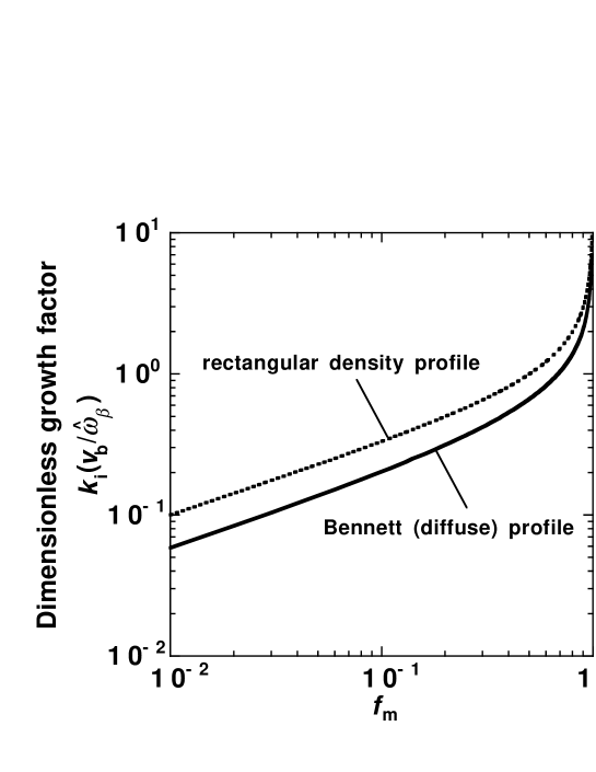
Figure 1: The growth factor of a convective mode, $k_{\rm i}(\omega\tau_{\rm d}\rightarrow 0)$, multiplied by $v_{\rm b}/{\hat{\omega}}_{\beta}$ as a function of $f_{\rm m}$, for the rectangular radial density profile (equation 8; dotted curve) and the diffuse radial density profile for the modified Bennett pinch equilibrium (equation 15; solid curve). Here, $\tau_{\rm d}$ is the resistive decay time (equations 33 and 41), $v_{\rm b}$ is the beam velocity, ${\hat{\omega}}_{\beta}$ is the betatron frequency at the beam centre $r=0$ (equation 12), and $f_{\rm m}$ is the ratio of the return/beam current density.

Fig. 1 plots the dimensionless growth factor $(-\chi)^{1/2}$ as a function of $f_{\rm m}$ for $0.01\leq f_{\rm m}<1$, together with, for comparison, the function of $k_{\rm i}(v_{\rm b}/{\hat{\omega}}_{\beta})=[f_{\rm m}/(1-f_{\rm m})]^{1/2}$ for the case of the rectangular radial density profile (Section 5.1.1). When the current neutral condition is perfectly satisfied [i.e. $\beta=0$ ($f_{\rm m}=1$)], the value of $k_{\rm i}=({\hat{\omega}}_{\beta}/v_{\rm b})[-\chi(f_{\rm m})]^{1/2}$ diverges, whereas no return current ($f_{\rm m}=0$) trivially leads to $k_{\rm i}=0$. It is, again, found that the repulsive interaction between the beam current and the return current is essential for driving the instability. As seen in Fig. 1, the present value of $k_{\rm i}$ is smaller than that obtained for the rectangular density profile. Namely, the diffuse boundary effects extend the growth distance of $L=2\pi/k_{\rm i}$. However, the effects are not so significant that the expected value of $L$ is found to be much shorter than the length-scale of astrophysical jets (cf. equation 34). More importantly, the pair production effects significantly lower the value of ${\hat{\omega}}_{\beta}$, thereby decreasing $k_{\rm i}$; however, the value of $L$ seems to be still much shorter than the observed length of the jets.

5.2.2 Mode property for complex $\omega$ and real $\Omega$

In parallel to Section 5.1.2, we examine the complex $\omega$ and real $\Omega$ case, referred to as the absolute mode. Because of real $\Omega$, $x$ $(=\Omega^{2}/{\hat{\omega}}_{\beta}^{2})$ is real and positive, so that $G(x;g=0)$ is also real. For $g\neq 0$ (for $0<x<1$), both $k_{z}$ and $\omega$ are complex, which may be expressed as $k_{z}={\rm i}k_{\rm i}+k_{\rm r}$ and $\omega={\rm i}\omega_{\rm i}+\omega_{\rm r}$. Recalling equations (40) and (42), and the relation $\Omega=\omega-k_{z}v_{\rm b}$, we have $k_{\rm i}=\omega_{\rm i}/v_{\rm b}$ and $k_{\rm r}=(\omega_{\rm r}-\Omega)/v_{\rm b}$, which can, respectively, be expressed as

$$k_{\rm i}=\frac{1}{v_{\rm b}\tau_{\rm d}}\frac{G_{0}(x)+f_{\rm m}}{1-f_{\rm m}},$$ (43)

where $G_{0}(x)\equiv G(x;g=0)$, and

$$k_{\rm r}=-\frac{1}{v_{\rm b}}\left[g\pi\frac{6x^{2}\left(1-x\right)}{\left(1-f_{\rm m}\right)\tau_{\rm d}}+{\rm sgn}(\Omega){\hat{\omega}}_{\beta}\sqrt{x}\right].$$ (44)

On the RHS of equation (44), the first term inside the square bracket is ordinarily much smaller than the second term, whereupon equation (44) can be approximated by equation (36). The positive value of $k_{\rm i}$ can be compared to the growth factor for the absolute mode, but, importantly, equation (43) does not contain the resonance point of $x$ that appeared in the rectangular density profile (Section 5.1.2).

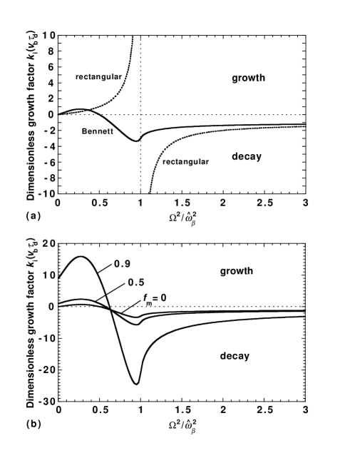
Figure 2: The growth factor of the absolute mode, $k_{\rm i}$, multiplied by $v_{\rm b}\tau_{\rm d}$ as a function of $\Omega^{2}/{\hat{\omega}}_{\beta}^{2}$, indicating (a) for $f_{\rm m}=0$, a comparison in between the rectangular profile (equation 35; dotted curve) and modified Bennett profile (equation 43; solid curve) cases, and (b) the $f_{\rm m}$-dependence for the latter case. Here, $\Omega$ $(\equiv\omega-k_{z}v_{\rm b})$ is the frequency of perturbations viewed in the beam frame. In (a), for the rectangular case the resonant point exists at $\Omega^{2}/{\hat{\omega}}_{\beta}^{2}=1$ (vertical thin dashed line). Note that the solid curve in (a) and the curve for $f_{\rm m}=0$ in (b) correspond to the function $G(\Omega^{2}/{\hat{\omega}}_{\beta}^{2};g=0)$ (equation 42; Uhm & Lampe 1980).

Fig. 2(a) plots, for the special case of $f_{\rm m}=0$, the dimensionless growth factor $k_{\rm i}(v_{\rm b}\tau_{\rm d})$ of equation (43) as a function of $x$ in the range $x\geq 0$, together with, for comparison, equation (35) for the rectangular profile case. It is noted that for $f_{\rm m}=0$, the function $k_{\rm i}(v_{\rm b}\tau_{\rm d})$ of equation (43) reduces to $G_{0}(x)$, recalling fig. 2 in Uhm & Lampe (1980) and fig. 9.16 in Davidson (1990). As $G_{0}(x\rightarrow 0)=0$ and $G_{0}(x\rightarrow+\infty)=-1$, in equation (43) we find $k_{\rm i}(x\rightarrow 0)=(v_{\rm b}\tau_{\rm d})^{-1}[f_{\rm m}/(1-f_{\rm m})]$ and $k_{\rm i}(x\rightarrow+\infty)=-(v_{\rm b}\tau_{\rm d})^{-1}$; these asymptotic values coincide with those of equation (35). As seen in Fig. 2(a), in the range $0<x<1$, the growth factor for the rectangular case is always positive, whereas the diffuse effects arrange an $x$-domain in which the stable condition, $k_{\rm i}\leq 0$, is satisfied. Note that $G_{0}(x=\frac{1}{2})=0$; in the range $0<x<\frac{1}{2}$, $G_{0}(x)>0$ takes the maximum value of $G_{0,\rm max}=0.690$ at $x=0.272$, whereas in the range $x>\frac{1}{2}$, $G_{0}(x)<0$ takes the minimum value of $G_{0,\rm min}=-3.36$ at $x=0.949$. In particular, for $x>0.635$, $G_{0}(x)<-1$, so that the stable condition, $k_{\rm i}<0$, is always satisfied for the possible range of $f_{\rm m}$.

Fig. 2(b) plots, for $f_{\rm m}=0$, $0.5$ and $0.9$, $k_{\rm i}(v_{\rm b}\tau_{\rm d})$ (equation 43) as a function of $x$. It is clearly found that when the return current increases (i.e. with increasing $f_{\rm m}$), the maximum (minimum) value of $k_{\rm i}(v_{\rm b}\tau_{\rm d})$, which is achieved at the common $x$-point of $x|_{G_{0}=G_{0,{\rm max}}}$ ($x|_{G_{0}=G_{0,{\rm min}}}$), enormously increases (decreases). In contrast to the infinite divergence at $x=1$ involved in equation (35), $G_{0,\rm max}$ is found to provide the finite maximum value of $k_{\rm i}$ [i.e. $k_{\rm i,max}\simeq(v_{\rm b}\tau_{\rm d})^{-1}(0.7+f_{\rm m})(1-f_{\rm m})^{-1}$ at $x\simeq 0.27$], where equation (44) approximately reads $k_{\rm r}\simeq-{\rm sgn}(\Omega)0.52{\hat{\omega}}_{\beta}/v_{\rm b}$. Namely, the growth factor is bounded; physically, this is because there is no single frequency $\Omega$ for which the entire beam is resonant with the wave (Uhm & Lampe, 1980). The values of $k_{\rm i,max}$ and $k_{\rm r}$ determine the shortest growth distance of wave envelope defined by $L_{\rm min}\equiv 2\pi/k_{\rm i,max}$ and the corresponding oscillation wavelength of the carrier wave, $\lambda_{\rm osc}\equiv 2\pi/|k_{\rm r}|$, respectively. These are explicitly written as

$$L_{\rm min}=\frac{\pi^{2}\beta_{\rm b}r_{\rm b}^{2}{\hat{\sigma}}}{c}\frac{1-f_{\rm m}}{0.7+f_{\rm m}},$$ (45)

$$\lambda_{\rm osc}=\frac{12v_{\rm b}}{{\hat{\omega}}_{\beta}}.$$ (46)

In the derivation of equation (45), equation (33) has been employed as the expression of $\tau_{\rm d}$. The obtained result suggests that astrophysical jets can propagate over, at least, the distance of $\sim L_{\rm min}$, having the spatial oscillation with the wavelength of $\lambda_{\rm osc}$ $(\ll L_{\rm min})$.

Let us evaluate equation (45). Concerning the electrical conductivity, for simplicity we here employ the standard Spitzer formula. In the regime of $T\gg m_{\rm e}c^{2}$ likely for pair plasmas, we have the relation ${\hat{\sigma}}/\sigma_{\rm S}\sim[(2\pi)^{1/2}/8](m_{\rm e}c^{2}/T)^{1/2}$, where $\sigma_{\rm S}\sim T^{3/2}/(e^{2}m_{\rm e}^{1/2}\ln\Lambda)$ is the well-known non-relativistic Spitzer conductivity (Braams & Karney, 1987; Honda, 2003); that is, for the Coulomb logarithm of $\ln\Lambda\sim 10$ (e.g. Huba, 1994), the scaling of ${\hat{\sigma}}\sim 10^{12}(T/10^{10}~{}{\rm K})~{}{\rm s^{-1}}$. We also call the relation $(1-f_{\rm m})/(0.7+f_{\rm m})=\beta/(1.7f_{\rm b}\beta_{\rm b}-\beta)$. Then, using equations (16) and the above expression of ${\hat{\sigma}}$ for $T\gg m_{\rm e}c^{2}$, equation (45) is found to scale as

$$L_{\rm min}=2.7\eta\left(\frac{10}{\ln\Lambda}\right)\left(\frac{1~{}{\rm cm^{-3}}}{{\hat{n}}_{\rm b}}\right)\left(\frac{T}{10^{10}~{}{\rm K}}\right)^{2}~{}{\rm Mpc},$$ (47)

while for $T\ll m_{\rm e}c^{2}$, setting to ${\hat{\sigma}}=\sigma_{\rm S}$, yields

$$L_{\rm min}=1.1\times 10^{2}\eta\left(\frac{10}{\ln\Lambda}\right)\left(\frac{1~{}{\rm cm^{-3}}}{{\hat{n}}_{\rm b}}\right)\left(\frac{T}{10^{8}~{}{\rm K}}\right)^{5/2}~{}{\rm pc}.$$ (48)

Here, the enhancement factor is introduced, defined as

$$\eta\equiv\frac{1-\left(\Delta f_{\rm pair}/2\right)}{\beta\Delta f_{\rm pair}^{2}\left[1-\left(\beta/1.7f_{\rm b}\beta_{\rm b}\right)\right]},$$ (49)

which takes a value in the range $\eta\geq 2/(1.7f_{\rm b}\beta_{\rm b})$. The strong $T$-dependence of equations (47) and (48) arises from that of $r_{\rm b}^{2}\propto T$, and ${\hat{\sigma}}\propto T$ (for $T\gg m_{\rm e}c^{2}$) or $T^{3/2}$ (for $T\ll m_{\rm e}c^{2}$).

In the regimes of $\Delta f_{\rm pair}/2\ll 1$ and $\beta/(1.7f_{\rm b}\beta_{\rm b})\ll 1$, equation (49) can be approximated by $\eta\simeq 1/(\beta\Delta f_{\rm pair}^{2})\gg 1$. In particular, for $\Delta f_{\rm pair}/2\ll 1$, the factor $\eta$ is reciprocal to $\Delta f_{\rm pair}^{2}$ (i.e. proportional to the square of the pair production rate), reflecting that the radial expansion stemming from the charge screening effects by positrons ($r_{\rm b}\propto\Delta f_{\rm pair}^{-1}$) significantly increases the value of $\tau_{\rm d}$, to extend $L_{\rm min}$. For $\beta<0.85f_{\rm b}\beta_{\rm b}$, $\eta$ increases with decreasing $\beta$, and particularly for $\beta\ll 1.7f_{\rm b}\beta_{\rm b}$, $\eta\propto\beta^{-1}$; this implies that the radial expansion effect ($r_{\rm b}\propto\beta^{-1}$) tends to surpass the destabilization by the return current. Even for the special case of $f_{\rm b}=1$ and $\beta=\beta_{\rm b}$ ($f_{\rm m}=0$), equations (47) and (48) are valid, having $\eta=(2.4/\beta_{\rm b})[1-(\Delta f_{\rm pair}/2)]/\Delta f_{\rm pair}^{2}$ ($\geq 1.2$).

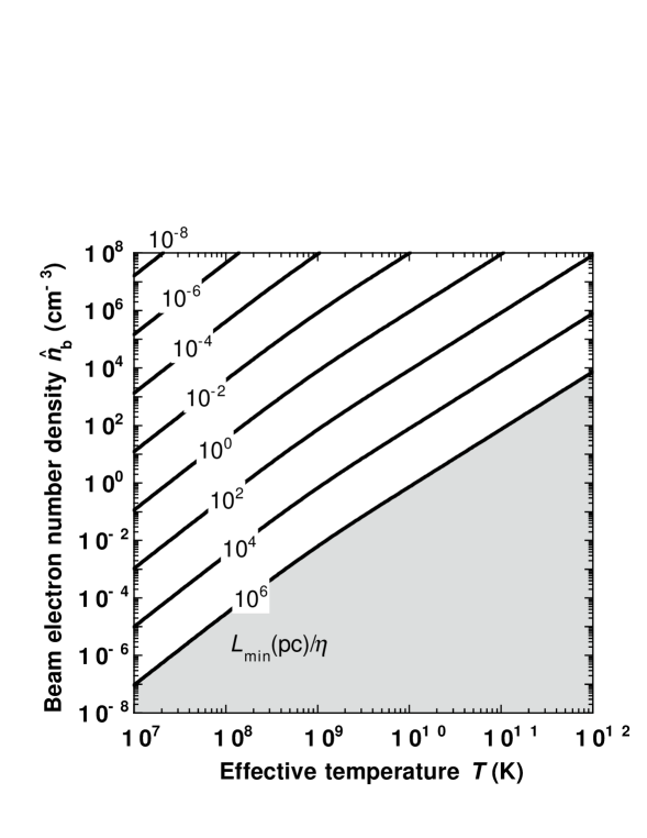
Figure 3: The contour plots of $L_{\rm min}/\eta$ for the values of $10^{-8}-10^{6}~{}{\rm pc}$ (labelled) in the ${\hat{n}}_{\rm b}-T$ parameter space, for the Bennett profile case in Fig. 2 (exhibiting the maxima $k_{\rm i,max}$). Here, $L_{\rm min}$ is the shortest growth distance (defined by $L_{\rm min}\equiv 2\pi/k_{\rm i,max}$; equation 45), $\eta$ $(>1)$ is the enhancement factor (equation 49), ${\hat{n}}_{\rm b}$ is the beam electron number density at $r=0$, and $T$ is the effective temperature (equation 4). The shaded area indicates the (${\hat{n}}_{\rm b}$, $T$)-parameter domain where supra-Mpc-scale transport is allowed for $\eta\sim 1$.

Fig. 3 plots ${\hat{n}}_{\rm b}$ as a function of $T$, for the given parameter $L_{\rm min}/\eta$ in the range $10^{-8}-10^{6}~{}{\rm pc}$. Here, the generic formulae of ${\hat{\sigma}}$ is used, which covers the mild relativistic region (Braams & Karney, 1987; Honda, 2003) and $\ln\Lambda$ dependent weakly on density and temperature (e.g. for ${\hat{n}}_{\rm b}\geq 1~{}{\rm cm^{-3}}$ and $T\leq 10^{10}~{}{\rm K}$, $\ln\Lambda\la 30$; Huba, 1994). The shaded area indicates the (${\hat{n}}_{\rm b}$, $T$)-parameter domain in which Mpc-scale transport of jets is safely achieved even for the marginal (most pessimistic) case of $\eta\sim 1$. Such a parameter domain more significantly expands for the larger values of $\eta$ owing to, for example, the larger pair production rate. As a consequence, it can be claimed that there is a wide parameter domain in which relativistic outflow can safely propagate up to $1~{}{\rm Mpc}$ corresponding to the observed longest scale of extragalactic jets. Also, for fixed $\eta$, the smaller $L_{\rm min}$ allows the flow to possess lower $T$ and higher ${\hat{n}}_{\rm b}$, that is, expanding the allowable (${\hat{n}}_{\rm b}$, $T$)-parameter domain. This property seems to be reflected in small-scale jets such as Galactic jets, comprising lower temperature, electron–ion plasma with $T\ll m_{\rm e}c^{2}$ and $f_{\rm pair}=0$ ($\Delta f_{\rm pair}=1$).

6 DISCUSSION AND CONCLUSIONS

As investigated above, absolute growth can be allowed, particularly for the case of the diffuse radial density profile reflecting the Bennett pinch-type equilibrium. However, in a low-frequency and/or high-resistivity regime, the characteristic distance of the convective growth is, for both the rectangular density and Bennett profiles, much shorter than the observed length of astrophysical jets, even if the pair production rate is large enough to lower the betatron frequency ${\hat{\omega}}_{\beta}$. Hence, the actual development of the convective mode appears to be ruled out. A simple explanation for the reason why the mode could not crucially evolve is that the condition for zero return current, namely $f_{\rm m}=0$, is perfectly satisfied inside the beam (Honda et al., 2000a). Also, if the mean poloidal (axial) magnetic field, $B_{0}{\bf\hat{z}}$, is superimposed to arrange the helical field (e.g. Asada et al., 2002; Gabuzda & Chernetskii, 2003), as well as the plasma wall in the vacuum channel (Section 1) being in close proximity to the beam, the mode can be stabilized (Uhm & Lampe, 1980; Davidson, 1990). For example, for the rectangular profile case, the sufficient condition for instability can be written as

$$f_{\rm m}>\frac{\left(r_{\rm b}/b\right)^{2}+\varrho^{2}}{1+\varrho^{2}},$$ (50)

where $b$ $(>r_{\rm b})$ is the radial distance from $r=0$ to the plasma wall, $\varrho\equiv\omega_{\rm cb}/(2{\hat{\omega}}_{\beta})$, and $\omega_{\rm cb}\equiv eB_{0}/(\gamma_{\rm b}m_{\rm e}c)$ is the relativistic cyclotron frequency. It turns out, in equation (50), that the aforementioned cases of either $f_{\rm m}=0$, $\varrho^{2}\gg 1$ realized for a larger $B_{0}$ (or a smaller $\gamma_{\rm b}$) or $r_{\rm b}/b\sim 1$ lead to the robust stabilization. Another possible explanation is that because the plasma is likely non-uniform in actual environments, the mode can be continuously carried away from the unstable (to stable) region. However, the absolute growing mode tends to be retained at the region where the unstable condition is satisfied, thereby the instability can evolve (but note again that in the present context, the growth factor will be favorably small, as reflected in equations 47 and 48). Note that a similar mode-preference is known to appear in laboratory plasmas establishing non-uniformity.

Along with equation (50), once the aforementioned necessary steps are taken to stabilize the convective mode, the stability properties of the absolute mode also change. Similar to the convective mode, for example. for the rectangular profile case, the larger values of $r_{\rm b}/b$ and $f_{\rm m}=0$ have a stabilizing influence on the absolute mode. The superimposition of $B_{0}\neq 0$ yields different effects: shifting the range of $\Omega(=\omega-k_{z}v_{b})$ corresponding to instability relative to the $B_{0}=0$ case, and expanding the bandwidth $(\omega_{\rm cb}^{2}+{\hat{\omega}}_{\beta}^{2})^{1/2}$ of the instability in the $\Omega$-space (Davidson, 1990). It appears that these effects are not significant enough to disturb the reasoning that the convective mode must be somehow strongly suppressed or stabilized in the actual system.

In conclusion, a full derivation has been given of the eigenvalue equation for the kink-type perturbations superimposed on the relativistic electron–positron beam with the modified Bennett and rectangular profiles. The dispersion relations have been examined for the convective and absolute modes of the resistive hose instability. It has been shown explicitly that the pair production effects lower the betatron frequency ${\hat{\omega}}_{\beta}$ and expand the beam filament radius $r_{\rm b}$. The following key results are found.

1. The reduction of ${\hat{\omega}}_{\beta}$ leads to a reduction of the growth factor of a convective mode scaled as $k_{\rm i}\sim{\hat{\omega}}_{\beta}/v_{\rm b}$.

2. The expansion of $r_{\rm b}$ prolongs the resistive decay time for perturbed current $\tau_{\rm d}$ ($\propto r_{\rm b}^{2}$; equation 33), resulting in a reduction of the growth factor of the absolute mode scaled as $k_{\rm i}\sim 1/(v_{\rm b}\tau_{\rm d})$.

For typical parameters, we found ${\hat{\omega}}_{\beta}\gg 1/\tau_{\rm d}$, implying that the convective growth is dominant, although its enormously rapid evolution, which ought to disrupt jets, appears to be incompatible with the observational facts because of the possible interpretation given above.

The Bennett profile effects also suppress the convective growth, but the growth distance is still much shorter than the observed length of jets (even if the positron effects are involved). In addition, the effects remove, for the absolute mode, the resonant divergence of the growth factor, and the growth distance is found to be comparable to (or longer than) the length-scale of jets. To summarize these consequences, preferentially, (i) actual evolution of the convective mode, in a low frequency and/or high resistivity regime, is ruled out and (ii) evolution of the absolute mode is allowed, more safely for the Bennett profile case. Closer inspections by observations, laboratory experiments and kinetic simulations are awaited.

Appendix A DERIVATION OF MODIFIED EIGENVALUE EQUATION

In this appendix, we derive an eigenvalue equation that governs equations (31) and (37). According to the method of characteristics (Krall & Trivelpiece, 1986; Davidson, 1990), we begin by integrating equation (26) from $z^{\prime}=-\infty$ to $z^{\prime}=z$. Neglecting the initial perturbation at $z^{\prime}=-\infty$, we obtain

$$\delta f_{\rm b}({\bf p},r,\theta,z,\tau)=\frac{e}{c}\frac{p_{z}}{p_{\perp}}\frac{\partial f_{\rm b}^{0}({\bf p},r)}{\partial p_{\perp}}\int_{-\infty}^{z}\frac{{\rm d}z^{\prime}}{v_{\rm b}}$$

$$\times\left(v_{r}^{\prime}\frac{\partial}{\partial r^{\prime}}+\frac{v_{\theta}^{\prime}}{r^{\prime}}\frac{\partial}{\partial\theta^{\prime}}\right)\delta A_{z}[r^{\prime}(z^{\prime}),\theta^{\prime}(z^{\prime}),z^{\prime},\tau].$$ (51)

Using $v_{r}^{\prime}=v_{\rm b}\left({\rm d}r^{\prime}/{\rm d}z^{\prime}\right)$ and $v_{\theta}^{\prime}=r^{\prime}v_{\rm b}\left({\rm d}\theta^{\prime}/{\rm d}z^{\prime}\right)$, and equations (29) and (30), equation (51) can be written as

$$\delta f_{\rm b}({\bf p},r)=\frac{e}{c}\frac{p_{z}}{p_{\perp}}\frac{\partial f_{\rm b}^{0}({\bf p},r)}{\partial p_{\perp}}\int_{-\infty}^{z}{\rm d}z^{\prime}\left(\frac{{\rm d}r^{\prime}}{{\rm d}z^{\prime}}\frac{\partial}{\partial r^{\prime}}+\frac{{\rm d}\theta^{\prime}}{{\rm d}z^{\prime}}\frac{\partial}{\partial\theta^{\prime}}\right)$$

$$\times\delta A_{z}[r^{\prime}(z^{\prime})]\exp\left\{{\rm i}\left[\theta^{\prime}(z^{\prime})-\theta\right]-{\rm i}\frac{\Omega}{v_{\rm b}}\left(z^{\prime}-z\right)\right\}.$$ (52)

In terms of the generic function of $\delta{\cal F}[r^{\prime}(z^{\prime}),\theta^{\prime}(z^{\prime}),z^{\prime}]$, we utilize the chain rule for differentiation: ${\rm d}\delta{\cal F}/{\rm d}z^{\prime}=\left[\left({\rm d}r^{\prime}/{\rm d}z^{\prime}\right)\left(\partial/\partial r^{\prime}\right)+\left({\rm d}\theta^{\prime}/{\rm d}z^{\prime}\right)\left(\partial/\partial\theta^{\prime}\right)+\partial/\partial z^{\prime}\right]\delta{\cal F}$. Then, we have

$$\delta f_{\rm b}({\bf p},r)=\frac{e}{c}\frac{p_{z}}{p_{\perp}}\frac{\partial f_{\rm b}^{0}({\bf p},r)}{\partial p_{\perp}}\int_{-\infty}^{z}{\rm d}z^{\prime}\left(\frac{\rm d}{{\rm d}z^{\prime}}+{\rm i}\frac{\Omega}{v_{\rm b}}\right)$$

$$\times\delta A_{z}[r^{\prime}(z^{\prime})]\exp\left\{{\rm i}\left[\theta^{\prime}(z^{\prime})-\theta\right]-{\rm i}\frac{\Omega}{v_{\rm b}}\left(z^{\prime}-z\right)\right\}.$$ (53)

When we impose $\theta^{\prime}(z^{\prime}=z)=\theta$ and $r^{\prime}(z^{\prime}=z)=r$, and recall $\left[\delta A_{z}(r^{\prime})\right]_{z^{\prime}=-\infty}=0$, the integration of equation (53) gives

$$\delta f_{\rm b}({\bf p},r)=\frac{e}{c}\frac{p_{z}}{p_{\perp}}\frac{\partial f_{\rm b}^{0}({\bf p},r)}{\partial p_{\perp}}\left[\delta A_{z}(r)+{\rm i}\frac{\Omega}{v_{\rm b}}\int_{-\infty}^{z}{\rm d}z^{\prime}\right.$$

$$\left.\times\delta A_{z}[r^{\prime}(z^{\prime})]\exp\left\{{\rm i}\left[\theta^{\prime}(z^{\prime})-\theta\right]-{\rm i}\frac{\Omega}{v_{\rm b}}\left(z^{\prime}-z\right)\right\}\right].$$ (54)

Substituting equation (54) into equation (25) concomitant with the replacement of $\partial/\partial t\rightarrow\partial/\partial\tau$, we obtain

$$\left[\frac{1}{r}\frac{\partial}{\partial r}\left(r\frac{\partial}{\partial r}\right)-\frac{1}{r^{2}}+\frac{4\pi{\rm i}\omega\sigma(r)}{c^{2}}\right]\delta A_{z}(r)$$

$$=4\pi e^{2}\beta_{\rm b}^{2}{\hat{n}}_{\rm b}\Delta f_{\rm pair}\int_{0}^{\infty}{\rm d}U\frac{\partial}{\partial U}F_{\rm b}(H)$$

$$\times\left[\delta A_{z}(r)+\frac{\Omega}{v_{\rm b}}I(\Omega,r,U)\right],$$ (55)

where the orbit integral $I$ is defined as

$$I(\Omega,r,U)\equiv{\rm i}\int_{0}^{2\pi}\frac{{\rm d}\phi}{2\pi}\int_{-\infty}^{0}{\rm d}\zeta\delta A_{z}[r^{\prime}(z^{\prime})]$$

$$\times\exp\left\{{\rm i}\left[\theta^{\prime}(z^{\prime})-\theta\right]-{\rm i}\frac{\Omega}{v_{\rm b}}\zeta\right\}.$$ (56)

Here, $\zeta=z^{\prime}-z$, and $\phi$ is the perpendicular momentum phase, conforming to $p_{x}+{\rm i}p_{y}=p_{\perp}(\cos\phi+{\rm i}\sin\phi)$.

Concerning the unknown function $\delta A_{z}[r^{\prime}(z^{\prime})]$ in the integrand of equation (56), it is known that, for $|\omega|\tau_{\rm d}<1$ (where $\tau_{\rm d}$ is the resistive decay time; cf. equations 33 and 41), $\delta A_{z}(r^{\prime})=\delta A_{z}(r)r^{\prime}/r$ provides a reasonably good approximation in the beam interior permeated by the magnetic field of $B_{\theta}^{\rm s}\propto r$ (Davidson, 1990). Physically, such a solution reflects a rigid displacement of the magnetic field. Putting the approximate expression of $\delta A_{z}(r^{\prime})$ into equation (56), the betatron orbit expression $r^{\prime}(z^{\prime})\exp\left[{\rm i}\theta^{\prime}(z^{\prime})\right]$ arises in the integrand. As usual, this can be expanded by solving the equation of motion of $\{v_{\rm b}({\rm d}^{2}/{\rm d}z^{\prime^{2}})+\omega_{\beta}^{2}[r^{\prime}(z^{\prime})]\}[x^{\prime}(z^{\prime})+{\rm i}y^{\prime}(z^{\prime})]=0$. After the manipulation, the orbit can be described as

$$r^{\prime}(z^{\prime})\exp\left[{\rm i}\theta^{\prime}(z^{\prime})\right]=(1/2)\left[r\exp({\rm i}\theta)+{\rm i}\omega_{\beta}^{-1}(p_{\perp}/\gamma_{\rm b}m_{\rm e})\right.$$

$$\left.\times\exp({\rm i}\phi)\right]\left[\exp(-{\rm i}\omega_{\beta}\zeta/v_{\rm b})-\exp({\rm i}\omega_{\beta}\zeta/v_{\rm b})\right].$$ (57)

As for the integrand of the RHS of equation (55), we invoke the density inversion theorem (cf. Section 3.2), which gives

$$\int_{0}^{\infty}{\rm d}U\frac{\partial}{\partial U}F_{\rm b}\left(H\right)=\left[\frac{\partial\psi_{\rm b}(r)}{\partial r}\right]^{-1}\frac{1}{{\hat{n}}_{\rm b}}\frac{\partial n_{\rm b}^{0}(r)}{\partial r}.$$ (58)

Making use of equations (57) and (58), equation (55) (involving equation 56) can be integrated, to finally yield

$$\frac{\partial}{\partial r}\frac{1}{r}\frac{\partial}{\partial r}r\delta A_{z}(r)+\frac{4\pi{\rm i}\omega\sigma(r)}{c^{2}}\delta A_{z}(r)$$

$$=-\frac{4\pi e^{2}\beta_{\rm b}^{2}\Delta f_{\rm pair}}{\gamma_{\rm b}m_{\rm e}}\frac{\delta A_{z}(r)}{\left(\Omega^{2}-\omega_{\beta}^{2}\right)}\frac{1}{r}\frac{\partial n_{\rm b}(r)}{\partial r}.$$ (59)

The form of equation (59) is similar to that of equation (45) in Uhm & Lampe (1980), but in the RHS of the present equation (59) we have the corrections related to the pair production rate, that is, the factor $\Delta f_{\rm pair}$ and the correction via $\omega_{\beta}^{2}$ given in equations (12) or (22).

References

- Alfvén (1939) Alfvén H., 1939, Phys. Rev., 55, 425
- Alfvén (1981) Alfvén H., 1981, Cosmic Plasma. Reidel, Dordrecht
- Appl & Camenzind (1992) Appl S., Camenzind M., 1992, A&A, 256, 354
- Asada et al. (2002) Asada K., Inoue M., Uchida Y., Kameno S., Fujisawa K., Iguchi S., Mutoh M., 2002, PASJ, 54, L39
- Asada et al. (2006) Asada K., Kameno S., Shen Z.-Q., Horiuchi S., Gabuzda D. C., Inoue M., 2006, PASJ, 58, 261
- Bahcall et al. (1995) Bahcall J. N., Kirhakos S., Schneider D. P., Davis R. J., Muxlow T. W. B., Garrington S. T., Conway R. G., Unwin S. C., 1995, ApJ, 452, L91
- Benford (1978) Benford G., 1978, MNRAS, 183, 29
- Bennett (1934) Bennett W. H., 1934, Phys. Rev., 45, 890
- Braams & Karney (1987) Braams B. J., Karney C. F. F., 1989, Phys. Fluids B 1, 1355
- Bridle & Perley (1984) Bridle A. H., Perley R. A., 1984, ARA&A, 22, 319
- Britzen et al. (2005) Britzen S. et al., 2005, A&A, 444, 443
- Buneman (1958) Buneman O., 1958, Phys. Rev. Lett., 1, 8
- Capetti et al. (1999) Capetti A., Axon D. J., Macchetto F. D., Marconi A., Winge C., 1999, ApJ, 516, 187
- Carilli & Barthel (1996) Carilli C. L., Barthel P. D., 1996, A&AR, 7, 1
- Chandrasekhar (1981) Chandrasekhar S., 1981, Hydrodynamic and Hydromagnetic Stability. Dover, New York
- Conway et al. (1993) Conway R. G., Garrington S. T., Perley R. A., Biretta J. A., 1993, A&A, 267, 347
- Davidson (1990) Davidson R. C., 1990, Physics of Nonneutral Plasmas. Addison Wesley, Palo Alto, CA
- Fleishman (2006) Fleishman G. D., 2006, MNRAS, 365, L11
- Frank et al. (1996) Frank A, Jones T. W., Ryu D., Gaalaas J. B., 1996, ApJ, 460, 777
- Gabuzda & Chernetskii (2003) Gabuzda D. C., Chernetskii V. A., 2003, MNRAS, 339, 669
- Hanasz & Sol (1996) Hanasz M., Sol H., 1996, A&A, 315, 355
- Hardee (2004) Hardee P. E., 2004, Ap&SS, 293, 117
- Heyl (2001) Heyl J. S., 2001, Phys. Rev. D, 63, 064028
- Honda (2000) Honda M., 2000, Phys. Plasmas, 7, 1606
- Honda (2003) Honda M., 2003, Phys. Plasmas, 10, 4177
- Honda (2004) Honda M., 2004, Phys. Rev. E, 69, 016401
- Honda & Honda (2002) Honda M., Honda Y. S., 2002, ApJ, 569, L39
- Honda & Honda (2004) Honda M., Honda Y. S., 2004, ApJ, 617, L37
- Honda & Honda (2005) Honda M., Honda Y. S., 2005, ApJ, 633, 733
- Honda & Honda (2007) Honda M., Honda Y. S., 2007, ApJ, 654, 885
- Honda et al. (2000a) Honda M., Meyer-ter-Vehn J., Pukhov A., 2000a, Phys. Plasmas, 7, 1302
- Honda et al. (2000b) Honda M., Meyer-ter-Vehn J., Pukhov A., 2000b, Phys. Rev. Lett., 85, 2128
- Huba (1994) Huba J. D., 1994, NRL Plasma Formulary. The Office of Naval Research, Washington, DC
- Joyce & Lampe (1983) Joyce G., Lampe M., 1983, Phys. Fluids, 26, 3377
- Junor et al. (1999) Junor W., Biretta J. A., Livio M., 1999, Nat, 401, 891
- Krall & Trivelpiece (1986) Krall N. A., Trivelpiece A. W., 1986, Principles of Plasma Physics. San Francisco Press, CA
- Lobanov & Zensus (2001) Lobanov A. P., Zensus J. A., 2001, Sci, 294, 128
- Malagoli et al. (1996) Malagoli A., Bodo G., Rosner R., 1996, ApJ, 456, 708
- Nishikawa et al. (2003) Nishikawa K.-I., Hardee P., Richardson G., Preece R., Sol H., Fishman G. J., 2003, ApJ, 595, 555
- Owen et al. (1989) Owen F. N., Hardee P. E., Cornwell T. J., 1989, ApJ, 340, 698
- Perley et al. (1984) Perley R. A., Dreher J. W., Cowan J. J., 1984, ApJ, 285, L35
- Potash & Wardle (1980) Potash R. I., Wardle J. F. C., 1980, ApJ, 239, 42
- Reynolds et al. (1996) Reynolds C. S., Fabian A. C., Celotti A., Rees M. J., 1996, MNRAS, 283, 873
- Roland & Hermsen (1995) Roland J., Hermsen W., 1995, A&A, 297, L9
- Swain et al. (1998) Swain M. R., Bridle A. H., Baum S. A., 1998, ApJ, 507, L29
- Treichel et al. (2001) Treichel K., Rudnick L., Hardcastle M. J., Leahy J. P., 2001, ApJ, 561, 691
- Uhm & Lampe (1980) Uhm H. S., Lampe M., 1980, Phys. Fluids, 23, 1574
- Uhm & Lampe (1981) Uhm H. S., Lampe M., 1981, Phys. Fluids, 24, 1553
- Wardle et al. (1998) Wardle J. F. C., Homan D. C., Ojha R., Roberts D. H., 1998, Nat, 395, 457
- Wilks et al. (2005) Wilks S. C. et al., 2005, Ap&SS, 298, 347
- Xie et al. (1995) Xie G. Z., Liu B. F., Wang J. C., 1995, ApJ, 454, 50
- Yusef-Zadeh & Morris (1987) Yusef-Zadeh F., Morris M., 1987, ApJ, 322, 721
- Yusef-Zadeh et al. (1984) Yusef-Zadeh F., Morris M., Chance D., 1984, Nat, 310, 557
- Yusef-Zadeh et al. (2004) Yusef-Zadeh F., Hewitt J., Cotton W., 2004, ApJS, 155, 421
- Zdziarski & Lightman (1985) Zdziarski A. A., Lightman A. P., 1985, ApJ, 294, L79