Evidence for overdensity around $z_{\rm em}$ $>$ 4 quasars from the proximity effect

Abstract

We study the density field around $z_{\rm em}$ $>$ 4 quasars using high quality medium spectral resolution ESI-Keck spectra ($R$ $\sim$ 4300, SNR $>$ 25) of 45 high-redshift quasars selected from a total of 95 spectra. This large sample considerably increases the statistics compared to previous studies. The redshift evolution of the mean photo-ionization rate and the median optical depth of the intergalactic medium (IGM) are derived statistically from the observed transmitted flux and the pixel optical depth probability distribution function respectively. This is used to study the so-called proximity effect, that is, the observed decrease of the median optical depth of the IGM in the vicinity of the quasar caused by enhanced photo-ionization rate due to photons emitted by the quasar. We show that the proximity effect is correlated with the luminosity of the quasars, as expected. By comparing the observed decrease of the median optical depth with the theoretical expectation we find that the optical depth does not decrease as rapidly as expected when approaching the quasar if the gas in its vicinity is part of the standard IGM. We interpret this effect as revealing gaseous overdensities on scales as large as $\sim$15$h^{-1}$ Mpc. The mean overdensity is of the order of two and five within, respectively, 10 and 3$h^{-1}$ Mpc. If true, this would indicate that high redshift quasars are located in the center of overdense regions that could evolve with time into massive clusters of galaxies. The overdensity is correlated with luminosity: brighter quasars show higher overdensities.

1 Introduction

The Inter-Galactic Medium (IGM) has been intensively studied using the absorption seen in the spectra of quasi-stellar objects (QSOs) over a large redshift range ($0.16\leq z_{\rm em}\leq 6.3$). This absorption, first identified by Lynds (1971), breaks up at high spectral resolution in hundreds of discrete absorption lines from, predominantly, HI Lyman UV resonance lines redshifted in a expanding universe (the so-called Ly$\alpha$ forest, see Rauch 1998 for a review).

The Ly$\alpha$ forest was interpreted by Sargent et al. (1980) as the signature of intervening HI clouds of cosmological nature embedded in a diffuse hot medium. The clouds were further described by Rees (1986) as gravitationally confined by dark-matter mini-halos. The advent of numerical simulations has introduced a new and more general scheme in which the IGM is a crucial element of large scale structures and galaxy formation. It is now believed that the space distribution of the gas traces the potential wells of the dark matter. In addition, most of the baryons are in the IGM at high redshift, making the IGM the reservoir of gas for galaxy formation. The numerical $N$-body simulations have been successful at reproducing the observed characteristics of the Ly$\alpha$ forest (e.g., Cen et al. 1994; Petitjean et al. 1995; Hernquist et al. 1996; Theuns et al. 1998). The IGM is therefore seen as a smooth pervasive medium which can be used to study the spatial distribution of the mass on scales larger than the Jeans’ length. This idea is reinforced by observations of multiple lines of sight (e.g., Coppolani et al. 2006).

It is well known that the characteristics of the Ly$\alpha$ forest change in the vicinity of the quasar due to the additional ionizing flux produced by the quasar. The mean neutral hydrogen fraction decreases when approaching the quasar. Because the amount of absorption in the IGM is, in general, increasing with redshift, this reversal in the cosmological trend for redshifts close to the emission redshift of the quasar is called the ’inverse’ or ’proximity’ effect (Carswell et al. 1982; Murdoch et al. 1986). It is possible to use this effect, together with a knowledge of the quasar luminosity and its position, to derive the mean flux of the UV background if one assumes that the redshift evolution of the density field can be extrapolated from far away to close to the quasar. Indeed, the strength of the effect depends on the ratio of the ionization rates from the quasar and the UV background, and because the quasar’s ionization rate can be determined directly through the knowledge of its luminosity and distance, the ionization rate in the IGM can be inferred. This method was pioneered by Bajtlik, Duncan & Ostriker (1988) but more recent data have yielded a wide variety of estimates (Lu, Wolfe & Turnshek 1991; Kulkarni & Fall 1993; Bechtold 1994; Cristiani et al. 1995; Fernandez-Soto et al. 1995; Giallongo et al. 1996; Srianand & Khare 1996; Cooke, Espey & Carswell 1997; Scott et al. 2000, 2002; Liske & Williger 2001). Scott et al. (2000) collected estimates from the literature which vary over almost an order of magnitude at $z=3$. The large scatter in the results can be explained by errors in the continuum placement, cosmic variance, redshift determination, etc.

In the standard analysis of the proximity effect it is assumed that the underlying matter distribution is not altered by the presence of the quasar. The only difference between the gas close to the quasar or far away from it is the increased photoionization rate in the vicinity of the QSO. If true, the strength of the proximity effect should correlate with the quasar luminosity but such a correlation has not been convincingly established (see Lu et al. 1991; Bechtold 1994; Srianand & Khare 1996; see however Liske & Williger 2001). It is in fact likely that the quasars are located inside overdense regions. Indeed, the presence of Ly$\alpha$ absorption lines with $z_{\rm abs}$ $>$ $z_{\rm em}$ suggests an excess of material around QSOs (Loeb & Eisenstein 1995; Srianand & Khare 1996). Furthermore, in hierarchical models of galaxy formation, the supermassive black holes that are thought to power quasars are located in massive haloes (Magorrian et al. 1998; Ferrarese 2002), that are strongly biased to high-density regions. Possible evidence for overdensities around quasars come also from studies of the transverse proximity effect by Croft (2004), Schirber, Miralda-Escudé & McDonald (2004) and Worseck & Wisotzki (2006) who suggest that the observed absorption is larger than that predicted by models assuming standard proximity effect and isotropic quasar emission. However, in the case of transverse observations, it could be that the quasar light is strongly beamed in our direction or, alternatively, that the quasar is highly variable. Interestingly, neither of these affects the longitudinal proximity effect discussed in the present paper.

Observations of the IGM transmission close to Lyman break galaxies (LBGs) seem to show that, close to the galaxy, the IGM contains more neutral hydrogen than on average (Adelberger et al. 2003). As the UV photons from the LBGs cannot alter the ionization state of the gas at large distances, it is most likely that the excess absorption is caused by the enhanced IGM density around LBGs. It is worth noting however that various hydrodynamical simulations have trouble reproducing this so-called galaxy proximity effect (e.g., Bruscoli et al. 2003; Kollmeier et al. 2003; Maselli et al. 2004; Desjacques et al. 2004).

In a recent paper, Rollinde et al. (2005) presented a new analysis to infer the density structure around quasars. The method is based on the determination of the cumulative probability distribution function (CPDF) of pixel optical depth, and so avoids the Voigt profile fitting and line counting which is traditionally used (e.g., Cowie & Songaila 1998; Ellison et al. 2000; Aguirre et al. 2002; Schaye et al 2003; Aracil et al. 2004; Pieri et al. 2006). The evolution in redshift of the optical depth CPDF far away from the quasar is directly derived from the data. This redshift dependent CPDF is then compared to the CPDF observed close to the quasar to derive the mean density profile around quasars. The method was applied to twenty lines of sight toward quasars at $z_{\rm em}\sim 2$ observed with UVES/VLT and it was found that overdensities of the order of a few are needed for the observations to be consistent with the value of the UV background flux derived from the mean Ly$\alpha$ opacity. In the present paper we apply the same method to a large sample of 95 quasars at $z_{\rm em}$ $>$ 4 observed with the Echelle Spectrograph and Imager (ESI) mounted on the Keck II telescope.

In Section 2 we describe the data and the selection of the sample used in the present work. We derive the redshift evolution of the ionizing UV background and of the median IGM optical depth in Sections 3 and 4 respectively. We discuss the proximity effect in Section 5 and conclude in Section 6. We assume throughout this paper a flat Universe with $\Omega_{\rm m}$ = 0.3, $\Omega_{\rm\Lambda}$ = 0.7, $\Omega_{\rm b}$ = 0.04 and H_o = 70 kms^-1.

2 Data and sample selection

Medium resolution (R $\sim$ 4300) spectra of all $z>3$ quasars discovered in the course of the DPOSS survey (Digital Palomar Observatory Sky Survey; see, e.g., Kennefick et al. 1995, Djorgovski et al. 1999 and the complete listing of QSOs available at http://www.astro.caltech.edu/$\sim$george/z4.qsos) have been obtained with the Echellette Spectrograph and Imager (ESI, Sheinis et al 2002) mounted on the KECK II 10 m telescope. Signal-to-noise ratio is usually larger than 15 per 10 km s^-1 pixel . These data have already been used to construct a sample of Damped Ly$\alpha$ systems at high redshift (Prochaska et al. 2003a,b). In total, 95 quasars have been observed.

The KECK/ESI spectra were reduced (bias subtraction, flat-fielding, spectrum extraction) using standard procedures of the IRAF package. The different orders of the spectra were combined using the scombine task. In the Echellette mode spectra are divided in ten orders covering the wavelength range: $4000$ Å $\leq\lambda_{\rm obs}\leq$ 10000 Å. In this work we use only orders 3 (center 4650 Å) to 7 (center 6750 Å). The spectral resolution is $R\sim 4300$ or $\sim 70$ km s^-1. During the process of combining the orders, we controlled carefully the signal-to-noise ratio obtained in each order. Wavelengths and redshifts were computed in the heliocentric restframe and the spectra were flux calibrated and then normalized.

The signal-to-noise ratio per pixel was obtained in the regions of the Ly-$\alpha$ forest that are free of absorption and the mean SNR value, averaged between the Ly-$\alpha$ and Ly-$\beta$ emission lines, was computed. We used only spectra with mean SNR $\geq$ 25. We rejected the broad absorption line QSOs (BAL) and QSOs with more than one damped Ly$\alpha$ system (DLA) redshifted between the Ly-$\alpha$ and the Ly-$\beta$ emission lines because their presence may over-pollute the Ly$\alpha$ forest. Metal absorptions are not subtracted from the spectra. We can estimate that the number of intervening CIV and MgII systems with $W_{\rm obs}$ $>$ 0.25 Å  is of the order of five along each of the lines of sight (see e.g., Boksenberg et al. 2003; Aracil et al. 2004; Tytler et al. 2004; Scannapieco et al. 2006). This means we expect an error on the determination of the mean absorption of the order of 1 %. This is at least five times smaller than the error expected from the placement of the continuum.

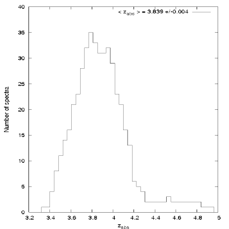
Figure 1: Number of spectra in our sample contributing to the study of the Ly-$\alpha$ forest at a given redshift as a function of redshift.

In Table 1 we give the characteristics of the forty-five QSO spectra satisfying the above criteria that are used in the present work. Column (1) gives the QSO’s name; column (2) the emission redshift estimated as the average of the determinations of the peak of the Ly$\alpha$ emission and the peak of a Gaussian fitted to the CIV emission line; column (3) the emission redshift obtained using the IRAF task rvidlines (see Section 5.1); column (4) the apparent V magnitude; column (5) the mean signal-to-noise ratio in the Ly$\alpha$ forest and column (6) the intrinsic luminosity at the Lyman limit estimated from the V-magnitude assuming that the QSO continuum spectrum is a power-law of index $-0.6$ (see Section 5). In Fig. 1 we show the histogram of the number of spectra in our sample contributing to the study of the Ly$\alpha$ forest at a given redshift as a function of redshift. Normalisation of the spectra is known to be a crucial step in these studies. An automatic procedure (Aracil et al. 2004) estimates iteratively the continuum by minimising the sum of a regularisation term (the effect of which is to smooth the continuum) and a $\chi^{2}$ term, which is computed from the difference between the quasar spectrum and the continuum estimated during the previous iteration. Absorption lines are avoided when computing the continuum. A few obvious defects are then corrected by hand adjusting the reference points of the fit. This happens to be important near the peak of strong emission lines and over damped absorption lines. The automatic method works very well and a minimal manual intervention is necessary. The procedure was calibrated by Aracil et al. (2004) using simulated quasar spectra (with emission and absorption lines) adding continuum modulations to mimic an imperfect correction of the blaze along the orders and noise to obtain a S/N ratio similar to that in the data. We noted that the procedure underestimates the true continuum in the Ly$\alpha$ forest by a quantity depending smoothly on the wavelength and the emission redshift by an amount of about 3-5% at $z$ $\sim$ 3.5-4. (see Fig. 1 of Aracil et al. 2004). This is less than our typical errors and therefore we did not correct the normalized spectra for this. Note that, due to strong blending, errors can be as high as 10% in places (see also Croft et al 2002; Becker et al. 2006; McDonald et al. 2006; Desjacques, Nusser & Sheth 2007). In that case however, the optical depth will be usually larger than the limit we will used to reject pixels badly affected by saturation. It must be noted also that, because of the reduced absorption in the vicinity of the quasar, the continuum determination is more reliable in the wing of the Ly$\alpha$ emission line. The normalization procedure we have used is preferred to other methods that are more arbitrary. It is completely reproducible and introduces only a small systematic error that we can control. A final sample reduced spectrum with the continuum fitting is shown in Fig. 2.

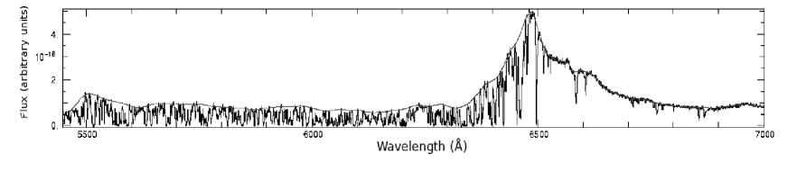
Figure 2: Flux calibrated spectrum of PSS 1058+1245. The continuum derived automatically is overplotted.

Table 1: Quasar sample

QSO	$z_{\rm em}$ a	$z_{\rm em}$ b	$V_{\rm mag}$	SNR	$L_{912}$ c
					$h^{-2}$ ergs s-1Hz-1
PSS0117+1552	4.241	4.244	18.6	45	4.53$\times$ 1031
PSS0118+0320	4.235	4.232	18.50	30	4.38$\times$ 1031
PSS0121+0347	4.130	4.127	17.86	72	6.76$\times$ 1031
SDSS0127-0045	4.067	4.084	18.37	25	4.04$\times$ 1031
PSS0131+0633	4.432	4.430	18.24	25	6.88$\times$ 1031
PSS0134+3307	4.534	4.536	18.82	30	4.73$\times$ 1031
PSS0209+0517	4.206	4.194	17.36	40	8.16$\times$ 1031
PSS0211+1107	3.975	3.975	18.12	66	6.14$\times$ 1031
PSS0248+1802	4.427	4.430	18.4	60	8.32$\times$ 1031
PSS0452+0355	4.397	4.395	18.80	30	4.77$\times$ 1031
PSS0747+4434	4.434	4.435	18.06	54	7.98$\times$ 1031
PSS0808+5215	4.476	4.510	18.82	37	4.29$\times$ 1031
SDSS0810+4603	4.078	4.074	18.67	43	3.22$\times$ 1031
PSS0852+5045	4.213	4.216	19	54	2.60$\times$ 1031
PSS0926+3055	4.188	4.198	17.31	77	1.22$\times$ 1032
PSS0950+5801	3.969	3.973	17.38	85	9.31$\times$ 1031
PSS0957+3308	4.283	4.274	17.59	40	9.80$\times$ 1031
PSS1057+4555	4.127	4.126	17.7	76	7.67$\times$ 1031
PSS1058+1245	4.332	4.330	18	46	7.45$\times$ 1031
PSS1140+6205	4.507	4.509	18.73	61	4.77$\times$ 1031
PSS1159+1337	4.089	4.081	18.50	45	3.65$\times$ 1031
PSS1248+3110	4.358	4.346	18.9	25	3.19$\times$ 1031
SDSS1310-0055	4.152	4.151	18.85	38	2.82$\times$ 1031
PSS1317+3531	4.370	4.369	19.10	28	2.75$\times$ 1031
J1325+1123	4.408	4.400	18.77	25	4.20$\times$ 1031
PSS1326+0743	4.121	4.123	17.3	66	1.01$\times$ 1032
PSS1347+4956	4.597	4.560	17.9	40	1.02$\times$ 1032
PSS1401+4111	4.008	4.026	18.62	30	2.90$\times$ 1031
PSS1403+4126	3.862	3.862	18.92	25	1.85$\times$ 1031
PSS1430+2828	4.309	4.306	19.30	40	2.18$\times$ 1031
PSS1432+3940	4.291	4.292	18.6	36	4.04$\times$ 1031
PSS1443+2724	4.419	4.406	19.3	30	2.57$\times$ 1031
PSS1458+6813	4.295	4.291	18.67	60	5.04$\times$ 1031
PSS1500+5829	4.229	4.224	18.6	40	3.74$\times$ 1031
GB1508+5714	4.306	4.304	18.9	32	3.12$\times$ 1031
PSS1535+2943	3.979	3.972	18.9	29	2.26$\times$ 1031
PSS1555+2003	4.226	4.228	18.9	31	3.15$\times$ 1031
PSS1633+1411	4.360	4.349	19.0	43	3.36$\times$ 1031
PSS1646+5514	4.110	4.084	18.11	37	4.81$\times$ 1031
PSS1721+3256	4.031	4.040	19.23	43	1.85$\times$ 1031
PSS1723+2243	4.515	4.514	18.17	42	8.77$\times$ 1031
PSS2154+0335	4.349	4.359	18.41	26	6.20$\times$ 1031
PSS2203+1824	4.372	4.375	18.74	34	4.50$\times$ 1031
PSS2238+2603	4.023	4.031	18.85	24	2.74$\times$ 1031
PSS2344+0342	4.341	4.340	17.87	30	4.38$\times$ 1031
a Mean of estimates from a Gaussian fit to the CIV emission line and from
the peak of the Ly$\alpha$ emission
b Estimate using the IRAF RVIDLINES task
c continuum luminosity at 912 Å

3 The Ionizing Background radiation field

The standard treatment of the proximity effect consists in studying the evolution of the mean absorption in the Ly$\alpha$ forest when approaching the quasar. Far away from the quasar the only source of ionizing photons is the UV background whereas in the vicinity of the quasar, the gas is ionized by both the UV background and the QSO. Assuming (i) that the luminosity of the quasar is known, (ii) that the distance from the gas to the quasar is cosmological (and therefore given by the difference in redshift) and (iii) that the density field in the IGM is not modified by the presence of the quasar, it is possible to derive observationally the distance to the quasar where the ionizing flux from the quasar equals the flux from the UV background. This, in turn, gives an estimate of the UV background flux. The last assumption neglects the fact that quasars can be surrounded by significant overdensities (e.g., Pascarelle et al. 2001; Adelberger et al. 2003; Rollinde et al. 2005; Faucher-Giguère et al. 2006; Kim & Croft 2006).

However the above approach can be reversed to derive the density distribution around the quasar if the UV background can be estimated from elsewhere. Actually, it is possible to estimate this flux by modelling the redshift evolution of the mean absorption in the IGM. For $z>4$ we can follow Songaila & Cowie (2002) and use the mean normalized transmitted flux, $F(z)$, to derive the normalized ionization rate, $g$, in units of 10^-12 s^-1, by inverting the following equation (see also McDonald & Miralda-Escudé 2001; Cen & McDonald 2002):

$$F(z)=4.5\times g^{-0.28}\times[\frac{(1+z)}{7}]^{2.2}\times e^{[-4.4g^{-0.4}[\frac{(1+z)}{7}]^{3}]}$$ (1)

with

$$g\equiv\Gamma_{-12}\times T_{4}^{0.75}\times h\times(\frac{\Omega_{\rm m}}{0.35})^{0.5}\times(\frac{\Omega_{\rm b}h^{2}}{0.0325})^{-2}$$ (2)

Applying the above equations, we can derive the redshift dependence of $\Gamma_{-12}$ from the observed transmitted flux (for $z>4$). For this, we have used the Ly$\alpha$ forest over the rest-wavelength range 1070-1170 Å  to avoid contamination by the proximity effect close to the Ly$\alpha$ emission line and by possible OVI associated absorbers. We also carefully avoided regions flagged because of data reduction problems or damped Ly$\alpha$ absorption lines. We divided each spectrum in bins of length $50$ Å  in the observed frame, corresponding to about $\triangle z=0.04$. The mean transmitted flux was calculated as the mean flux over all pixels in a bin. At each redshift, we then averaged the transmitted fluxes over all spectra covering this redshift. Errors were estimated as the standard deviation of the mean values divided by the square root of the number of spectra. The corresponding scatter in the transmitted flux cannot be explained by photon noise or by uncertainties in the continuum, suggesting that errors are dominated by cosmic variance. The mean transmitted flux that we have obtained is plotted in Fig 3 together with results by Songaila (2004).

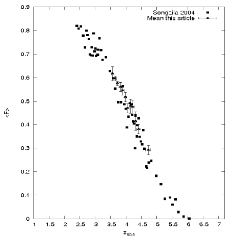
Figure 3: The observed normalized transmitted flux $<F>$ as a function of redshift.

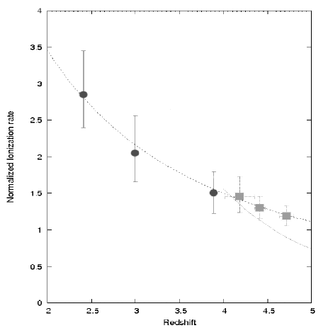
Figure 4: The normalized ionization rate obtained from the transmitted flux observed in our data by inverting Eq. 1 in three redshift bins (filled squares) at $z>4$. Filled circles are the measurements of McDonald et al. (2000) for lower redshift. The dotted line is a power law of the form $1.11\times[(1+z)/6]^{-1.63}$ fitted to the data of McDonald et al. (2000) and this paper. The dashed line is a power law of the form $0.74\times[(1+z)/6]^{-4.1}$ obtained, for $z>4$, by Songaila (2004).

The normalized ionization rate defined in Eq. 2 is derived from the mean normalized transmitted flux by inverting Eq. 1. Results are plotted in Fig. 4. To decrease the errors, we have used only three bins at $z>4$. It can be seen that our measurements are consistent with those by McDonald et al. (2000) at lower redshift. Fitting both McDonald’s and our results together, we find that the redshift evolution of $g$ is described as $g$ = 1.11$\times$[(1+z)/6]^-1.63. Note that our fit is not consistent with the results by Songaila (2004) who find $g$ = 0.74$\times$[(1+z)/6]^-4.1 for $z>4$. The corresponding photoionization rate, $\Gamma_{-12}$, in units of $10^{-12}$ s^-1, is given in Fig. 5, assuming $\Omega_{\rm b}h^{2}=0.019$, $\Omega_{\rm m}=0.3$ and three different values of gas temperature $T_{4}$ = 1, 1.5 and 2, in units of $10^{4}$ K. These results are consistent with the measurements by McDonald & Mirada-Escudé (2001) for a mean temperature of $T_{4}\sim$1.5 to 2 which is the mean temperature expected in the IGM at these redshifts. However, recent determination of this quantity (Becker et al. 2006) using a lognormal distribution for the optical depth distribution indicate that $\Gamma_{-12}$ could be higher by about a factor of two to three at these redshifts. We therefore have used in the following a mean temperature of $T_{4}=$ 1.

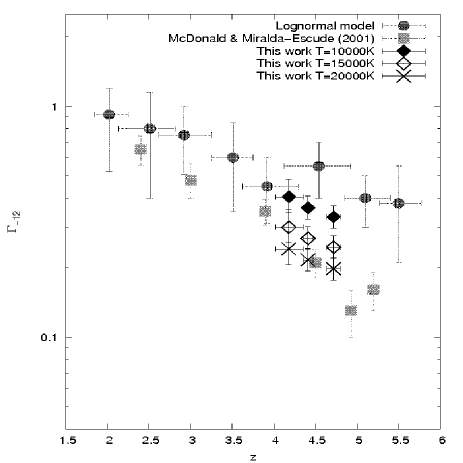
Figure 5: Redshift evolution of the photoinization rate, $\Gamma_{-12}$, derived from our data and using three different temperatures for the IGM, $T_{4}$ = 1.0, 1.5 and 2, in units of $10^{4}$ K (filled diamond, open diamond and crosses, respectively). Filled squares show the results by McDonald & Miralda-Escudé (2001) and filled circles the results from Becker et al. (2006). $\Omega_{\rm b}h^{2}=0.019$, $\Omega_{\rm m}=0.3$ are assumed here.

4 The Ly$\alpha$ optical depth statistics in the IGM

To study the influence of the additional ionizing flux from the quasar on the Ly$\alpha$ optical depth, we have first to derive the evolution of the optical depth with redshift in the IGM at large distances from the quasar. The observed HI opacity is simply:

$$\tau_{\rm HI}(\lambda)=-{\rm ln}(\frac{F_{\lambda_{\rm obs}}}{F_{\lambda_{\rm cont}}}),$$ (3)

where $F_{\lambda_{\rm obs}}$ is the observed flux and $F_{\lambda_{\rm cont}}$ is the flux in the continuum. Its evolution with redshift is described as

$$\tau\propto(1+z)^{\alpha}.$$ (4)

For each spectrum of the sample we estimate the optical depth, $\tau$, in each pixel between $\tau_{\rm min}=-{\rm ln}(1-3\sigma)$ and $\tau_{\rm max}=-{\rm ln}(3\sigma)$, where $\sigma(\lambda)$ is the rms of the noise measured in the spectrum (see column 5 of Table 1). We then construct the cumulative probability distribution of $\tau$ (CPDF) in redshift windows of approximately $\triangle z=0.04$ corresponding to $50$ Å  in the observed frame and estimate the associated percentiles. Because low and high values of the optical depth are lost either in the noise or because of saturation, we can use only the intermediate values of the percentiles. The evolutions with redshift of the 40, 50, 60 and 70 % percentiles are given in Fig. 6.

The redshift evolution index in Eq. 4 can be derived from the redshift evolution of the percentiles of the pixel optical depth CPDF (see Rollinde et al. 2005). The values obtained for $\alpha$ are ($5.8\pm 0.5$) for the 40 % percentile, ($5.1\pm 0.2$) for the 50 % percentile,($4.3\pm 0.2$) for the 60 % percentile and ($3.8\pm 0.4$) for the 70 % percentile. We use throughout the rest of the paper $\alpha$=4.8.

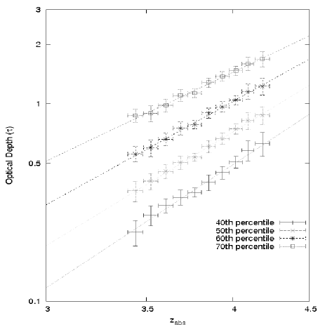
Figure 6: Redshift evolution of different percentiles derived from the CPDF of the pixel optical depth.

5 The proximity effect from optical depth statistics

The evolution with redshift of the optical depth in the IGM is inverted in the vicinity of the quasar due to the additional ionizing flux from the quasar. To disentangle the two effects we can correct the observed optical depth for the redshift evolution in the absence of the quasar by replacing $\tau_{\rm i}$ at redshift $z_{\rm i}$ by $\tau_{\rm i}$$\times$$[\frac{(1+z_{\rm ref})}{(1+z_{\rm i})}]^{\alpha}$, where $z_{\rm ref}$ is a fixed redshift taken as reference. We have corrected the observed optical depth for each pixel using the factor above with $z_{\rm ref}=4.5$ and the value of $\alpha$ obtained from the redshift evolution of the IGM CPDF, $\alpha$ = 4.8. The results are shown in Fig 7 (filled squares). The observed corrected median optical depth is given versus the distance to the quasar computed using the cosmological parameters given in Section 2 and assuming emission redshifts from column 3 of Table 1. The proximity effect is apparent as a decrease of the optical depth within a distance to the quasar smaller than $\sim$15-20 $h^{-1}$Mpc.

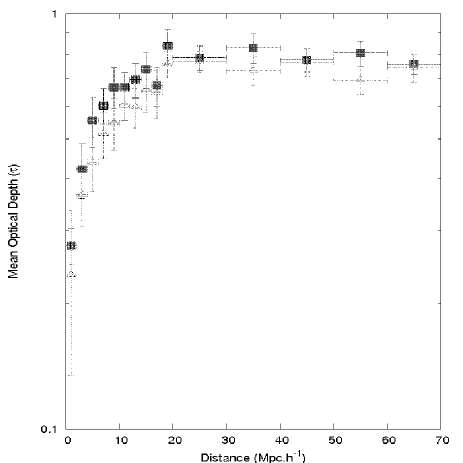
Figure 7: The median optical depth corrected for redshift evolution ($\tau\propto(1+z)^{\alpha}$ with $\alpha$ = 4.8) is given versus the distance to the quasar, derived using QSO emission redshifts from column 3 of Table 1 (filled squares). Open triangles correspond to the case where these redshifts are increased by an amount taken randomly between 0 and 1500 km s^-1.

5.1 QSO systemic redshifts

The above effect depends on the accurate determination of the QSO systemic redshift. Gaskell (1982) has shown that the redshifts derived from different quasar emission lines often do not agree with each other within typical measurement errors. The high-ionization broad emission lines (HILs; e.g., Ly$\alpha$ $\lambda 1215.67$, CIV $\lambda 1549$, CIII $\lambda 1909$ and NV $\lambda 1240$) are found systematically blueshifted with respect to the low-ionization broad emission lines (LILs; e.g, OI $\lambda 1305$, MgII $\lambda 2798$, and the permitted Balmer series) and principally from the forbidden narrow emission lines (e.g., NeV $\lambda 3426$, OII $\lambda 3727$, NeIII $\lambda 3870$, OIII $\lambda 5007$). The narrow emission lines arise from gas located in the galaxy host and their redshift should be more representative of the center-of-mass redshift (see e.g., Tytler & Fan 1992, Baker et al. 1994).

Unfortunately, for our sample of quasars with emission redshifts in the range $4\leq z_{\rm em}\leq 4.5$, the forbidden narrow emission lines cannot be detected from the ground because they are redshifted in near-infrared spectral windows that are absorbed by the terrestrial atmosphere. We have derived the emission redshifts using two approachs. In the first approach, the final redshift (see column 2 of Table 1) is the mean of two estimates: one obtained by fitting a Gaussian to the CIV emission line and the other by measuring the peak of the Ly$\alpha$ emission line to avoid the various absorption features shortwards of the line. In the second approach, the emission redshift (see column 3 of Table 1) was obtained using the IRAF task rvidlines. Initially we identify a prominent spectral feature (usually the Ly$\alpha$ emission line) to which a gaussian function is fitted. Based on the central wavelength of this line and an input list of known spectral features, other features at a consistent redshift are identified and fitted. The final emission redshift is a weighted average value based on the gaussian fits. The median optical depth of the IGM versus the distance to the quasar computed using emission redshifts obtained by this second approach is shown as squares in Fig. 7.

As we know that HILs are systematically blueshifted, with respect to LILs and narrow emission lines, from $500$ to $1500$ km s^-1 (Tytler & Fan 1992) we have increased the emission redshift (obtained by fitting the emission lines) by a random amount and calculated the optical depth versus the distance to the quasar as follows. For each realization, we increase the redshift of each of the 45 quasars by an amount taken randomly between 0 and 1500 km s^-1. We calculate the distance of each pixel of the lines of sight to the corresponding quasar and compute the median optical depth for each value of $r$ by averaging over all quasars. We then average the optical depths over a hundred realizations. Errors are taken as the mean rms obtained over the realizations. Results are shown in Fig. 7 (triangles). The proximity effect is more pronounced in that case, as expected. This approach will be used in the next Sections whenever we will use QSO emission redshifts.

5.2 The QSO ionization rate

The strength of the proximity effect depends on the ratio of the ionization rates from the QSO emission and the UV-background. The QSO ionization rate can be determined directly from its luminosity. The HI ionization rate due to a source of UV photons is formally given by the equation:

$$\Gamma_{\rm QSO}=\int_{\nu_{0}}^{\infty}[4\pi J_{\rm QSO}(\nu)\times\frac{\sigma_{\rm HI}(\nu)}{h\nu}].d\nu({\rm s}^{-1})$$ (5)

where, $\nu_{0}$ is the frequency of the Lyman limit, $\sigma_{\rm HI}(\nu)=6.3\times 10^{-18}(\frac{\nu_{0}}{\nu})^{3}$ cm² is the HI photo-ionization cross-section, $J_{\rm QSO}(\nu)=J_{\rm QSO}(\nu_{0})\times(\frac{\nu}{\nu_{0}})^{-\phi}$, if we assume that the ionizing spectrum is a power law of index $\phi$ and where, $J_{\rm QSO}(\nu_{0})$ is defined as:

$$4\pi\,J_{\rm QSO}(\nu_{0})=\frac{L_{\rm QSO}}{4\pi r^{2}}$$ (6)

with $L_{\rm QSO}$ the monochromatic luminosity of the quasar at the Lyman limit. These luminosities are computed extrapolating the flux in the continuum at $\lambda_{\rm obs}$ $\sim$ 6000 Å  using a power-law of index $\phi=-0.6$ (Francis et al. 1993). We checked that within a reasonable range of $\phi=-0.5$ to $-0.7$ (e.g., Cristiani & Vio 1990), our main result (i.e. the density structure around quasars) is not affected by this choice. Therefore,

$$\Gamma_{\rm QSO}=\frac{12.6\times 10^{-12}}{3+\phi}J_{\rm QSO}(\nu_{0})\,10^{21}({\rm s}^{-1})$$ (7)

thus,

$$\Gamma_{\rm QSO}^{12}\,=\,\frac{12.6}{3+\phi}\frac{L_{\rm QSO}/4\pi}{4\pi\,r^{2}}\,10^{21}(10^{-12}{\rm s}^{-1})$$ (8)

$r$ is the luminosity distance from the quasar of emission redshift $z_{\rm em}$ to the cloud at redshift $z$ and is calculated using equations given by Liske (2003) for a flat cosmological model.

5.3 Ionizing rate ratio

We define $\omega$ as the ratio of the ionizing rate due to the quasar emission to that due to the UV background, $\omega=\frac{\Gamma_{\rm QSO}(r,z)}{\Gamma_{\rm bck}(z)}$. The later has been derived in Section 4 (see Fig. 5). The enhanced ionizing flux in the vicinity of the QSO induces a decrease in the optical depth of the IGM observed in the absence of the QSO by a factor ($1+\omega$). For each spectrum, we have calculated $\omega_{\rm QSO}$ and $r$ for each pixel and then, at a given $r$, we have derived $\omega$ for the whole sample as the median of the individual values $\omega_{\rm QSO}$(r) found for each of the 45 quasars. The result is shown in Fig. 8.

Figure 8: The ratio $\omega=\frac{\Gamma_{\rm QSO}}{\Gamma_{\rm bck}}$ of the ionizing rate from the QSO to that from the UV background versus the cosmological distance between the quasar and the cloud in the IGM. $\Gamma_{\rm bck}$ is taken from Fig. 5.

5.4 Overdensities around the quasar

In the standard analysis of the proximity effect it is assumed that the matter distribution in the IGM is not altered by the presence of the quasar. The only difference between the gas located either close to the quasar or far away from it is the increased photo-ionization rate in the vicinity of the quasar. In that case, far away from the quasar, the median optical depth corrected for redshift evolution, $\tau_{\rm median}$, should be a constant we can call $\tau_{0}$. In the vicinity of a QSO, due to the emission of ionizing photons, $\tau_{\rm median}$ is no more a constant (see Fig. 7) and decreases when $r$ decreases as:

$$\tau_{\rm median}=\tau_{0}\frac{1}{(1+\omega)}$$ (9)

where $\omega$ was defined and derived in the previous Section (see Fig. 8).

The observed median optical depth $\tau_{\rm median}^{\rm obs}$ is compared to $\tau_{0}/(1+\omega)$ in Fig 9. It is apparent that the two curves do not agree and that the observed median optical depth is much larger than what would be expected in the case the density field of the IGM remains unperturbed when approaching the quasar. This means that on an average, there is an overdensity of gas compared to the IGM in the vicinity of the quasar.

If an overdensity, $\frac{\rho(r)}{\rho_{0}}$, is present around the quasar, then the median optical depth should be:

$$\tau_{\rm median}=\tau_{0}\frac{(\rho(r)/\rho_{0})^{[2-0.7(\gamma-1)]}}{(1+\omega)}$$ (10)

The $\gamma$ exponent has been shown by Schaye et al. (2000) to be in the range $\gamma$ = [1-1.5], thus it is reasonable to assume $\gamma$ = 1 for this work.

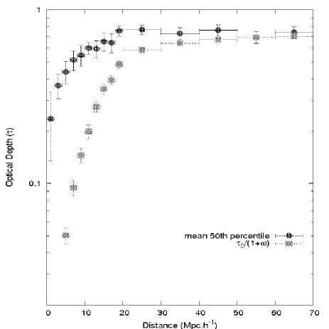
Figure 9: Comparison of median optical depth’s evolution observed close to the quasars (filled circles) with that of an evolution due to the ionization field of the quasar only (Eq. 10; filled squares). The difference between the curves can be interpreted as the presence of an overdensity of gas in the vicinity of the quasar.

Using Eq. 10 we can derive the actual overdensity. It is given versus the distance to the quasar in Fig. 10 (filled circles). The gas density close to the quasar is significantly higher than the mean density in the IGM at least within the first 10$h^{-1}$Mpc or so.

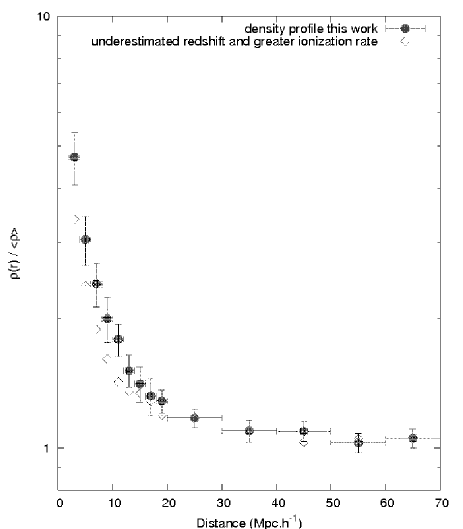
Figure 10: The mean density profile around quasars with emission redshift in the range $4\leq z_{\rm em}\leq 4.5$ as derived from this work is shown as filled circles. Open diamonds indicate the lower limit on the density profile derived assuming that the redshift from column 3 Table 1 is systematically underestimated by 1500 km s^-1 and that the ionizing rate in the IGM is that measured by Becker et al. (2006).

6 Discussion and Conclusions

In this paper we have used the method presented by Rollinde et al. (2005) to probe the density structure around quasars. In the vicinity of the quasar and in comparison with the situation far away from it, the ionization factor of the gas is increased by the emission of ionizing photons by the quasar and is decreased by the presence of an overdensity. If the redshift evolution of the IGM photo-ionization rate and that of the median optical depth in the IGM are both constrained by the observed evolution of the median optical depth in the Ly-$\alpha$ forest far from the quasar, then it is possible to derive the density structure in the vicinity of the quasar. We have followed McDonald & Miralda-Escudé (2001) to derive the mean ionization rate in the IGM at $z>4$. Our results are lower, by a factor of about 1.5, than the new results by Becker et al. (2006). We then have used the redshift evolution of the pixel optical depth PDF to estimate the redshift evolution of the median optical depth of the IGM. Using these results, we have found that quasars are surrounded by significant overdensities on scales up to about 10 $h^{-1}$Mpc. The overdensity is of the order of a factor of two at 10 $h^{-1}$Mpc but is larger than five within the first megaparsec. If true, we can estimate that the mass surrounding the quasars within 1 Mpc at this redshift is of the order of $10^{14}$ M_⊙ corresponding to the mass of a big cluster of galaxies.

An overdensity can be artificially derived from the above analysis if (i) the photo-ionization rate is underestimated and/or (ii) the redshift of the quasars are systematically underestimated for any reason. To check the robustness of our result we can try to obtain a lower limit on the overdensity surrounding the quasars. For this we have arbitrarily increased the photo-ionization rate that we used by a factor of 1.5 so that it is equal to the value obtained by Becker et al. (2006) at the same redshift. In addition, we have increased all quasar emission redshifts by 1500 km s^-1 to account for a possible systematic underestimate of the emission redshift when using the Ly-$\alpha$ emission line (note however that in our treatment we already increase the emission redshift from the Ly-$\alpha$ emission line by an amount taken randomly between 0 and 1500 km s^-1). The result is shown in Fig. 10 (open diamonds). It can be seen that the overdensity is still present although smaller as expected.

If our interpretation of the proximity effect is correct, we should expect a correlation between the strength of the observed proximity effect and the intrinsic luminosity of the QSOs. To test this effect, we have considered two subsets of our quasar sample, one containing the 15 QSOs with highest intrinsic luminosities ($6.14\times 10^{+31}\leq L\leq 1.22\times 10^{+32}$ $h^{-2}$erg s^-1Hz^-1) and the other containing the 17 QSOs with lowest intrinsic luminosities ($1.85\times 10^{+31}\leq L\leq 3.74\times 10^{+31}$ $h^{-2}$erg s^-1Hz^-1). We have avoided quasars with intermediate luminosities because they may dilute the possible result. In Fig. 11, we plot for both subsets the median optical depth versus the distance to the quasar. It is apparent that the proximity effect is less pronounced for the low-luminosity sample compared to the high-luminosity sample as expected. The Proximity effect is correlated with QSO luminosities. For illustration, we plot also $\tau_{0}/(1+\omega)$ for both subsets on the figure. The corresponding overdensities around the quasars in the two subsets are shown in Fig. 12. The overdensity is correlated with luminosity. Brighter quasars show higher overdensities. Some caution should be applied when interpreting this result however as we have used a quite simple model to correct the observed proximity effect.

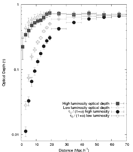
Figure 11: The median optical depth in versus the distance from the cloud to the quasar for two subsets of our QSO sample: one including the 15 QSOs of highest luminosities (filled squares) and the other including the 17 QSOs of lowest luminosities (open triangles). It is apparent that the proximity effect is correlated with luminosity as expected. The curves giving the factor (1 +$\omega$) are drawn for each subset for illustration (filled circles and open diamonds respectively.

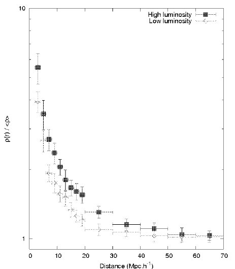
Figure 12: The density profile around quasars versus the distance from the cloud to the quasar for two subsets of our QSO sample: one including the 15 QSOs of highest luminosities (filled squares) and the other including the 17 QSOs of lowest luminosities (open diamonds).

At redshift $z\sim 2$, Rollinde et al. (2005) claimed tentative detection of overdensities of about a factor of two on scales $\sim$5$h^{-1}$ Mpc. The result was only marginal because the statistics was small. With a sample of 45 quasars at $z>4$, we have demonstrated that overdensities exist. This result strongly supports the idea that quasars at high redshift are located in regions of high overdensities probably flagging the places where massive clusters of galaxies will form.

It has been known for a long time that quasars are associated with enhancements in the distribution of galaxies (Bahcall, Schmidt & Gunn 1961) and that at low redshift ($z<0.4$) they are associated with moderate groups of galaxies (e.g., Fisher et al. 1996). However, little is known at high redshift. Our method yields a mean one-dimensional profile of the density distribution on large scales when other methods study the correlation of the quasar with surrounding objects (see Kauffmann & Haehnelt 2002). This result adds to the growing evidence that high-z QSOs seem to reside in dense and probably highly biased regions (Djorgovski 1999, Djorgovski et al. 1999). Observational efforts should be done to obtain deep images of the fields around bright high-$z$ quasars to search for the presence of any concentration of objects around the quasar.

Acknowledgements: RG is supported by a grant from the brazilian gouvernment (CAPES/MEC). AA is supported by a PhD grant from the Ministry of Science, Research &Technology of Iran. PPJ and RS gratefully acknowledge support from the Indo-French Centre for the Promotion of Advanced Research (Centre Franco-Indien pour la Promotion de la Recherche Avancée) under contract No. 3004-3. SGD is supported by the NSF grant AST-0407448, and the Ajax Foundation. Cataloguing of DPOSS and discovery of PSS QSOs was supported by the Norris Foundation and other private donors. We thank E. Thiébaut, and D. Munro for freely distributing his yorick programming language (available at ftp://ftp-icf.llnl.gov:/pub/Yorick), which we used to implement our analysis. The authors wish to recognize and acknowledge the very significant cutural role and reverence that the summit of Mauna Kea has always had within the indigenous Hawaian community. We are most fortunate to have the opportunity to conduct observations from this mountain. We acknowledge the Keck support staff for their efforts in performing these observations.

References

- [1] Adelberger K., Steidel C. C., Shapley A., Pettini M., 2003, ApJ, 584, 45
- [2] Aguirre, A., Schaye, J., & Theuns, T. 2002, ApJ, 576, 1
- [3] Aracil B., Petitjean P., Pichon C., Bergeron J., 2004, A&A, 419, 811
- [4] Bahcall J. N., Schmidt M., Gunn J. E., 1969, ApJ, 157, L77
- [5] Bajtlik S., Duncan R., Ostriker J., 1988, ApJ, 327, 570
- [6] Baker A. C., Carswell R. F., Bailey J. A., Espey B. R., Smith M. G., Ward M. J., 1994, MNRAS, 270, 575
- [7] Bechtold J. B., 1994, ApJS, 91, 1
- [8] Becker G. D., Rauch M., Sargent W. L. W., 2006, astro-ph/0607633
- [9] Boksenberg, A., Sargent, W. L. W., & Rauch, M. 2003, ArXiv Astrophysics e-prints, arXiv:astro-ph/0307557
- [10] Bruscoli M., Ferrara A., Marri S., Schneider R., Maselli A., Rollinde E., Aracil B., 2003, MNRAS, 343, 41
- [11] Carswell R. F., Whelan J., Smith M., Boksenberg A., Tytle, D., 1982, MNRAS, 198, 91
- [12] Cen R., Mc Donald P., 2002, ApJ, 570, 457
- [13] Cen R., Miralda-Escudé J., Ostriker J. P., Rauch M., 1994, ApJ, 437, 6
- [14] Cooke A. J., Espey B., Carswell R. F., 1997, MNRAS, 284, 552
- [15] Coppolani F., Petitjean P. Stoehr F., et al., 2006, MNRAS, 370, 1804
- [16] Cowie, L. L., & Songaila, A. 1998, Nat, 394, 44
- [17] Cristiani S., D’Odorico S., Fontana A., Giallongo E., Savaglio S., 1995, MNRAS, 273, 1016
- [18] Cristiani S., Vio R., 1990, A&A, 227, 385
- [19] Croft R., 2004, ApJ, 610, 642
- [20] Croft, R. A. C., Weinberg, D. H., Bolte, M., Burles, S., Hernquist, L., Katz, N., Kirkman, D., & Tytler, D. 2002, ApJ, 581, 20
- [21] Desjacques V., Nusser A., Haehnelt M. G., Stoehr F., 2004, MNRAS, 350, 879
- [22] Desjacques, V., Nusser, A., & Sheth, R. K. 2007, MNRAS, 374, 206
- [23] Djorgovski, S. G. 1999, in The High-Redshift Universe: Galaxy Formation and Evolution at High Redshift, eds. A.J. Bunker & W.J.M. van Breugel, ASPCS, 193, 397
- [24] Djorgovski, S. G., Odewahn, S. C., Gal, R. R., Brunner, R. J., & de Carvalho, R. R. 1999, ASP Conf. Ser. 191: Photometric Redshifts and the Detection of High Redshift Galaxies, 191, 179
- [25] Djorgovski, S. G., Gal, R. R., Odewahn, S. C., de Carvalho, R. R., Brunner, R., Longo, G., & Scaramella, R. 1999, in Wide Field Surveys in Cosmology, eds. S. Colombi, Y. Mellier, & B. Raban, Gif sur Yvette: Editions Frontières, p. 89
- [26] Djorgovski, S.G., Stern, D., Mahabal, A.A., & Brunner, R. 2003, ApJ, 596, 67
- [27] Ellison, S. L., Songaila, A., Schaye, J., & Pettini, M. 2000, AJ, 120, 1175
- [28] Faucher-Giguere, C. -., Lidz, A., Zaldarriaga, M., & Hernquist, L. 2007, ArXiv Astrophysics e-prints, arXiv:astro-ph/0701042
- [29] Fernandez-Soto A., Barcons X., Carballo R., Webb J. K., 1995, MNRAS, 277, 235
- [30] Ferrarese, L.,2002, ApJ, 578, 90
- [31] Fisher K. B., Bahcall J. N., Kirhakos S., Schneider D. P., 1996, ApJ, 468, 469
- [32] Francis P. J., Hooper E. J., Impey C. D., 1993, AJ, 106, 417
- [33] Gaskell C. M., 1982, ApJ, 263, 79
- [34] Giallongo E., Cristiani S., D’Odorico S., Fontana A., Savaglio S., 1996, ApJ, 466, 46
- [35] Hernquist L., Katz N., Weinberg D. H., 1996, ApJ, 457, 51
- [36] Kauffmann G., Haehnelt M., 2002, MNRAS, 332, 529
- [37] Kennefick, J.D., Djorgovski, S.G., & de Carvalho, R.R. 1995, AJ, 110, 2553
- [38] Kim, Y.-R., & Croft, R. 2006, ArXiv Astrophysics e-prints, arXiv:astro-ph/0701012
- [39] Kollmeier J. A., Weinberg D. H., Davé R., Katz N., 2003, ApJ, 594, 75
- [40] Kulkarni V. P., Fall S. M., 1993, ApJ, 413, 63
- [41] Liske, J. 2003, A&A, 398, 429
- [42] Liske J., Williger G. M., 2001, MNRAS, 328, 653
- [43] Loeb A., Eisenstein D., 1995, ApJ, 448, 17
- [44] Lu L., Wolfe A. M., Turnshek D. A., 1991, ApJ, 367, 19
- [45] Lynds R., 1971, ApJ, 164, L73
- [46] Magorrian J. et al., 1998, AJ, 115, 2285
- [47] Maselli A., Ferrara A., Bruscoli M., Marri S., Schneider R., 2004, MNRAS, 350, 21
- [48] McDonald P., & Miralda-Escudé J., 2001, ApJL, 549, 11
- [49] McDonald P., Miralda-Escudé J., Rauch M., et al., 2000, ApJ, 543, 1
- [50] McDonald, P., et al. 2006, ApJS, 163, 80
- [51] Murdoch H. S., Hunstead R. W., Pettini M., Blades J. C., 1986, ApJ, 309, 19
- [52] Pascarelle, S. M., Lanzetta, K. M., Chen, H.-W., & Webb, J. K. 2001, ApJ, 560, 101
- [53] Petitjean P., Mücket J. P., Kate R. E., 1995, A&A, 295, L9
- [54] Pieri, M. M., Schaye, J., & Aguirre, A. 2006, ApJ, 638, 45
- [55] Prochaska J.X., Gawiser E., Wolfe A., Castro S., Djorgovski S.G., 2003a, ApJ, 595, L9
- [56] Prochaska J.X., Castro S., Djorgovski S. G., 2003b, ApJS, 148, 317
- [57] Rauch M., 1998, ARA&A, 36, 267
- [58] Rees M. J., 1986, MNRAS, 218, 25
- [59] Rollinde E., Srianand R., Theuns T., Petitjean P., Chand H., 2005, MNRAS, 361, 1015
- [60] Sargent W. L. W., Young P. J., Boksenberg A., Tytler D., 1980, ApJS, 42, 41
- [61] Scannapieco, E., Pichon, C., Aracil, B., Petitjean, P., Thacker, R. J., Pogosyan, D., Bergeron, J., & Couchman, H. M. P. 2006, MNRAS, 365, 615
- [62] Schaye, J., Aguirre, A., Kim, T.-S., Theuns, T., Rauch, M., & Sargent, W. L. W. 2003, ApJ, 596, 768
- [63] Scott J., Bechtold J., Dobrzycki, A., Kulkarni V. P., 2000, ApJS, 130, 67
- [64] Scott J., Bechtold J., Morita M., Dobrzycki A., Kulkarni V. P., 2002, ApJ, 571, 665
- [65] Schaye, J., Theuns, T., Rauch, M., Efstathiou, G., & Sargent, W. L. W. 2000, MNRAS, 318, 817
- [66] Schirber M., Miralda-Escudé J., McDonald P., 2004, ApJ, 610, 105
- [67] Sheinis, A. I., et al., 2002, PASP, 114, 851
- [68] Songaila A., 2004, AJ, 127, 2598
- [69] Songaila A., & Cowie L., 2002, AJ, 123, 2183
- [70] Srianand R., Khare P., 1996, MNRAS, 280, 767
- [71] Theuns T., Leonard A., Efstathiou G., Pearce F. R., Thomas P. A., 1998, MNRAS, 301, 478
- [72] Tytler, D., et al. 2004, ApJ, 617, 1
- [73] Tytler D., Fan X. M., 1992, ApJS, 79, 1
- [74] Worseck G., Wisotzki L., 2006, A&A, 450, 495