The Accretion-Driven Structure and Kinematics of Relaxed Dark Halos

Abstract

It has recently been shown that relaxed spherically symmetric dark matter halos develop from the inside out, by permanently adapting their inner structure to the boundary conditions imposed by the current accretion rate. Such a growth allows one to infer the typical density profiles of halos. Here we follow the same approach to infer the typical spherically averaged profiles of the main structural and kinematic properties of triaxial, anisotropic, rotating halos. Specifically, we derive their density, spatial velocity dispersion, phase-space density, anisotropy and specific angular momentum profiles. The results obtained are in agreement with available data on these profiles from $N$-body simulations.

1 INTRODUCTION

High-resolution cosmological simulations show that relaxed cold dark matter (CDM) halos are close to triaxial homologous systems (Bailin & Steinmetz 2005) with a variety of axial ratios but essentially universal profiles. That is, the shape of the spherically averaged radial profile of any given structural and kinematic property is always very similar, independently of halo mass, epoch, environment and cosmology considered; only the scaling may depend on such particularities.

Dubinski & Carlberg (1991) and Crone et al. (1994) noted that halos of very different masses show similar scaled density profiles. Navarro et al. (1997, hereafter NFW) then showed that the spherically averaged density profile is always well fit, down to about one hundredth the virial radius $R$, by the simple expression

$$\langle\rho\rangle(r)\propto\frac{1}{r(r_{\rm s}+r)^{2}}\,,$$ (1)

with the scale radius $r_{\rm s}$ correlating with the total halo mass $M$ within $R$ in such a way that the smaller $M$, the higher the concentration $c\equiv R/r_{\rm s}$, a correlation that was interpreted (NFW; Salvador-Solé et al. 1998) as due to the fact that less massive halos typically form earlier when the mean cosmic density is higher.

Although there is nowadays general agreement on the previous universal density profile, some authors claim that higher resolutions yield slightly steeper central cusps (Fukushige & Makino 1997, 2001; Moore et al. 1998, 1999; Ghigna et al. 2000; Jing & Suto 2000; Diemand et al. 2004), while others advocate rather the opposite, that the density profile becomes shallower as smaller and smaller radii are reached (Taylor & Navarro 2001; Power et al. 2003; Fukushige et al. 2004; Hayashi et al. 2004). Zhao (1996) has proposed a more general practical expression that accounts for all these possibilities. Besides, it has more recently been shown (Navarro et al. 2004; Merritt et al. 2005; Merritt et al. 2006; Graham et al. 2006; see also Stoehr et al. 2002) that a new expression of the Sérsic (1968), in 3D, or Einasto (1965) law

$$\langle\rho\rangle(r)=\rho_{0}\exp\left[-\left(\frac{r}{r_{\rm n}}\right)^{1/n}\right]\,,$$ (2)

with strictly no central cusp, yields still better fits to the mass distribution of simulated halos. Down to the resolution-limited radii reached by current simulations, the discrepancies among all these analytical fits are of the order of the deviates found using any individual one (Dehnen & McLaughlin 2005; see also Navarro et al. 2004 and Fukushige et al. 2004), which explains such a diversity of opinions. In respect to the $c(M)$ relation, different analytical expressions have also been proposed that try to recover the results of numerical simulations at various redshifts (NFW; Eke, Navarro & Steinmetz 2001; Bullock et al. 2001a; Zhao et al. 2003). Again, there is overall agreement between them although the discrepancies become substantial as one gets apart from the mass and redshift ranges analyzed in simulations.

On the other hand, the 3D velocity dispersion profile $\sigma(r)$ is well fit by the solution of the Jeans equation for spherical, isotropic systems resulting from the empirical NFW density profile and vanishing velocity dispersion at infinity (Cole & Lacey 1996; see also Merritt et al. 2006 for the Einasto profile). What is more interesting, as noted by Taylor & Navarro (2001; see also Ascasibar et al. 2004; Rasia et al. 2004; Barnes et al. 2006), the (pseudo) phase-space density profile, $\langle\rho\rangle/\sigma^{3}$, is always close to a pure power law in radius

$$\frac{\langle\rho\rangle(r)}{\sigma^{3}(r)}=Ar^{-\nu}\,,$$ (3)

with index $\nu\approx 1.9$ (see also Dehnen & McLaughlin 2005 for a similar relation applying to the radial component of the velocity dispersion).

In addition, Hansen and Moore (2006) have recently shown that the pressure-supported anisotropy profile,

$$\beta(r)\equiv 1-\frac{\sigma_{\rm t}^{2}(r)}{\sigma_{\rm r}^{2}(r)}=\frac{1}{2}\left[3-\frac{\sigma^{2}(r)}{\sigma^{2}_{\rm r}(r)}\right]\,,$$ (4)

defined as usual in terms of the 1D radial and tangential velocity dispersion profiles, $\sigma_{\rm r}(r)$ and $\sigma_{\rm t}(r)$, respectively, is related to the logarithmic slope of the spherically averaged density profile through the simple linear relation

$$\beta(r)=a\left(\frac{{\rm d}\ln\langle\rho\rangle}{{\rm d}\ln r}+b\right)\,,$$ (5)

with constants $a$ and $b$ respectively equal to $\approx-0.2$ and $\approx 0.8$ (Hansen & Stadel 2006).

The simplicity of the relations (3) and (5) might suggest that they are more fundamental than the universal halo density and velocity dispersion profiles themselves. However, they appear to be equivalent: not only do the latter profiles satisfy the previous equations, but they are also the only profiles to do so. Indeed, the NFW density profile is the only physically acceptable, realistic (with no central hole), profile with Zhao’s (1996) general form that solves the Jeans equation satisfying the relation (3), both in the simple isotropic case (Austin et al. 2005; see also Taylor & Navarro 2001 and Hansen 2004) and the general anisotropic one, provided in this latter case the additional relation (5) (Dehnen & McLaughlin 2005).

Finally, cosmological simulations show that relaxed CDM halos have a small angular momentum, typically orientated along the minor axis of the inertia ellipsoid, whose modulus $J$ is log-normally distributed (e.g., Barnes & Efstathiou 1987; Ryden 1988; Warren et al. 1992; Cole & Lacey 1996; Bullock et al. 2001b, hereafter B01b; Bailin & Steinmetz 2005) in terms of the dimensionless spin parameters,

$$\lambda=\frac{J|E|^{1/2}}{GM^{5/2}}\,,$$ (6)

or

$$\lambda^{\prime}=\frac{J}{\sqrt{2}MRV_{\rm c}}=\frac{J}{M\sqrt{2GMR}}\,,$$ (7)

respectively defined by Peebles (1980) and B01b, where $G$ is the gravitational constant, $E$ is the total energy of the halo (with vanishing potential at infinity), $R$ is the virial radius and $V_{\rm c}\equiv\sqrt{GM/R}$ is the circular velocity. According to their respective definitions, both spin parameters would coincide provided halos were singular isothermal spheres, but for halos endowed with the NFW density profile, one has (B01b)

$$\lambda^{\prime}\approx\lambda F(c)\,,$$ (8)

with

$$F^{-2}(c)=\frac{2}{3}+\left(\frac{c}{21}\right)^{0.7}\,.$$ (9)

The mean $\lambda^{\prime}$ value appears to be essentially constant in time (Hetznecker & Burkert 2006) but dependent on halo mass, while the mean $\lambda$ value is independent of mass (B01b) but shows a slight variation in time (Hetznecker & Burkert 2006) due, in principle, to the evolution of halo concentration and mass distribution.

The local specific angular momentum vector within halos tends to be everywhere aligned (B01b), the cumulative mass-distribution of specific angular momenta $M(<j)$ being well fit by a simple two-parameter function and the spherically averaged specific angular momentum profile $\langle j\rangle(r)$ fairly well fit by the simple expression

$$\langle j\rangle(r)=\langle j\rangle(R)\,\left[\frac{M(r)}{M}\right]^{s}\,,$$ (10)

where $M(r)$ is the mass inside $r$ and index $s$ takes values around 1.3.

As argued by Austin et al. (2005), the equilibrium condition alone cannot explain all these universal trends because the Jeans equation is not restrictive enough, nor can the initial conditions, as very different protohalos lead to essentially the same final structural (Austin et al. 2005; Romano-Diaz et al. 2006) and kinematic (Hansen & Moore 2006) properties. Thus, what can only be at their origin is the way these systems grow and, in the case of the specific angular momentum profile, the effects of tidal torques suffered during that process (Doroshkevich 1970; White 1984).

Two extreme points of view have been investigated. Some authors have looked at the possibility that the universal density profile arises essentially from the effects of repeated mergers (Syer & White 1998; Salvador-Solé et al. 1998; Subramanian et al. 2000; Dekel et al. 2003). Others have focused on smooth accretion through spherical infall (Avila-Reese et al. 1998; Nusser & Sheth 1999; del Popolo et al. 2000; Manrique et al. 2003; Ascasibar et al. 2004). Similarly, the origin of the universal specific angular momentum profile has been studied in the spherical collapse approximation (B01b) or by considering the cumulative effect of mergers (Gardner 2001; Maller et al. 2002; Vitvitska et al. 2002).

A notable result found along this latter line of research is that the density profile predicted from spherical accretion resembles greatly that found in numerical simulations. However, major mergers cannot be ignored in any realistic hierarchical cosmology, which gives little credit to the “pure” accretion scenario. Yet, the density profiles of halos do not depend on the epoch they suffered the last major merger (Wechsler et al. 2002) nor, in general, on their particular aggregation history (Huss et al. 1999; Romano-Diaz et al. 2006). Manrique et al. (2003) pointed out that this would be well understood if the inner structure of relaxed halos were completely fixed by the boundary conditions imposed by current accretion and did not depend on the halo past history. In fact, taking into account that halos develop from the inside out during accretion phases (Salvador-Solé et al. 2005; Romano-Diaz et al. 2006; Lu et al. 2006), their typical density profile can be readily derived, in the spherically symmetric case, from the accretion rate characteristic of the cosmology under consideration (Manrique et al. 2003).

This accretion-driven density profile is in very good agreement with the results of numerical simulations in the whole radial, mass and redshift ranges reached by them (Salvador-Solé et al. 2007, hereafter SMGH) and recovers all the correlations shown by simulated halos such as the mass-concentration relation (Salvador-Solé et al. 2005). Furthermore, as recently shown by SMGH, all the conditions required in the derivation of this profile, but the spherical symmetry assumed for simplicity, emanate directly from the very nature of standard CDM. The fact that CDM is collisionless guarantees that the spatial distribution of any physical quantity is continuous at any derivative order. As a consequence, all halos with mass $M$ at the time $t$ undergoing the same accretion $\dot{M}(t)$ during some finite time interval around $t$ have identical (non-scaled) $M(r)$ and, hence, $\rho(r)$ profiles regardless of their individual past history. On the other hand, the non-decaying, non-self-annihilating and dissipationless nature of CDM added to the fact that it accretes slowly onto halos guarantees their inside-out growth. Finally, the CDM power-spectrum characteristic of the particular cosmology considered fixes the typical accretion rate and through it the typical density profile of relaxed halos of any given mass at any given cosmic time.

Yet, this success would be of limited interest if the same explanation did not also hold for the mass distribution in more realistic, triaxial halos and for any other property apart from the density. In the present paper, we show that this approach allows one to understand all the universal structural and kinematic trends of triaxial, velocity-anisotropic, rotating halos. In Section 2, we show that the total values at a given cosmic time of the extensive quantities characterizing relaxed halos and the rates at which they increase during any finite time interval around that moment determine completely the corresponding spherically averaged profiles. This is used, in Section 3, to infer the typical shape of these profiles. Our results are summarized and discussed in Section 4. Throughout the present paper we adopt the concordance cosmological model characterized by $(\Omega_{\rm m},\Omega_{\Lambda},h,\sigma_{8})=(0.3,0.7,0.7,0.9)$.

2 ACCRETION RATES AND UNIQUENESS OF PROFILES

Consider a relaxed (i.e. quasi-steady), triaxial, velocity-anisotropic, rotating dark matter halo. The mass inside radius $r$ takes the usual form for spherical systems,

$$M(r)=4\pi\int_{0}^{r}{\rm d}\tilde{r}\;\tilde{r}^{2}\;\langle\rho\rangle(\tilde{r})\,,$$ (11)

in terms of the spherically averaged density profile,

$$\langle\rho\rangle(r)=\frac{1}{4\pi}\int_{0}^{2\pi}\!\!{\rm d}\varphi\!\int_{0}^{\pi}\!\!{\rm d}\theta\;\sin\theta\;{\rho(r,\theta,\varphi)}\,,$$ (12)

where $\rho(r,\theta,\varphi)$ is the local density in spherical coordinates $r$, $\theta$ and $\varphi$, centered at the peak density and with $z$ axis orientated along the total angular momentum J within $R$.

The kinetic energy inside $r$ also takes the form for spherical systems (see the detailed derivation in the Appendix)

$$K(r)=4\pi\int_{0}^{r}{\rm d}\tilde{r}\,\tilde{r}^{2}\langle\rho\rangle(\tilde{r})\frac{\sigma^{2}(\tilde{r})}{2}\,,$$ (13)

in terms of the usual velocity-non-centered spatial velocity dispersion profile, $\sigma(r)$, which coincides with the spherical average of the local velocity dispersion $\sigma(r,\theta,\varphi)$ in the $r$ shell. Note that in dealing with non-centered velocity dispersions, the influence of rotation on the total kinetic energy of the system is included only implicitly in equation (13).

Simulations show that the local angular momentum vector is essentially aligned all over the halo, eventually except for the innermost and outermost regions respectively affected by the limited resolution and possible boundary effects due to the inclusion of infalling matter (B01b; Bailin & Steinmetz 2005). Consequently, the modulus $J$ of the total angular momentum vector inside $r$ can be written in terms of the modulus $j$ of the local specific one as

$$J(r)=\!\int_{0}^{r}\!\!{\rm d}\tilde{r}\,\tilde{r}^{2}\!\!\!\int_{0}^{2\pi}\!\!{\rm d}\varphi\!\int_{0}^{\pi}\!\!{\rm d}\theta\sin\!\theta\,j(r,\theta,\varphi)\,\rho(r,\theta,\varphi)\,.$$ (14)

Thus, using the spherical average profile,

$$\langle j\rangle(r)\!=\!\frac{1}{4\pi\langle\rho\rangle(r)}\!\!\int_{0}^{2\pi}\!\!\!\!{\rm d}\varphi\!\!\int_{0}^{\pi}\!\!{\rm d}\theta\sin\!\theta j(r,\theta,\varphi)\rho(r,\theta,\varphi),$$ (15)

it takes again the same form as for spherically symmetric systems,

$$J(r)=4\pi\int_{0}^{r}\!{\rm d}r\;r^{2}\,\langle j\rangle(r)\,\langle\rho\rangle(r)\,.$$ (16)

To conclude this preamble, let us add that the similarity with the spherically symmetric case when dealing with spherically symmetric profiles does not stop here. It also concerns, although only approximately, other profiles such as the potential energy inside $r$ or relations such as the Jeans equation and the scalar virial relation (see the Appendix). In particular, from equations (A10) and (A31) one has the relation

$$\sigma_{\rm r}^{2}(R)\!=\!\frac{1}{R^{3}\langle\rho\rangle(R)}\!\int_{0}^{R}\!\!\!{\rm d}r\,r^{2}\langle\rho\rangle(r)\left[\sigma^{2}(r)\!-\!\frac{GM(r)}{r}\right]\!.$$ (17)

2.1 Density Profile

As mentioned, relaxed halos evolve inside-out between major mergers, that is, they keep their inner density distribution unaltered and just stretch it outwards (Salvador-Solé et al. 2005; Romano-Diaz et al. 2006; Lu et al. 2006). This is the natural consequence of the fact that centered spheres of arbitrary radii conserve the mass (standard CDM is non-decaying and non-self-annihilating) and energy (standard CDM is dissipationless) and that the characteristic accretion time of halos is substantially smaller than their dynamical time (see SMGH). It is true that relaxed halos are triaxial, so they can in principle suffer tidal torques from the surrounding matter affecting the kinetic energy of such inner spheres. However, the tidal field produced by the surrounding anisotropic large scale mass distribution is very stable (possibly except for the short time interval before major mergers) and relaxed halos remain elongated along one fixed privileged direction. Consequently, tidal torques have a minimal effect on the internal kinematics of relaxed halos; they are only important near maximum expansion of protohalos where the angular momentum of those structures is generated.

The inside-out growth implies that, at any time $t$ during such accretion periods, the total mass is given by (see eq. (11])

$$M(t)\equiv M[R(t)]=4\pi\int_{0}^{R(t)}{\rm d}r\,r^{2}\langle\rho\rangle(r)\,,$$ (18)

where the function $\langle\rho\rangle$ inside the integral on the right is independent of time. Thus, by differentiating eq. (18) we are led to

$$\langle\rho\rangle(t)\equiv\langle\rho\rangle[R(t)]=\frac{\dot{M}}{4\pi R^{2}(t)\dot{R}}\,.$$ (19)

As the virial radius encompasses a region with inner mean density equal to some factor $\Delta_{\rm vir}(t)$ (e.g. Bryan and Norman 1998) times the mean cosmic density $\bar{\rho}(t)$,

$$R(t)=\left[\frac{3M(t)}{4\pi\Delta_{\rm vir}(t)\bar{\rho}(t)}\right]^{1/3}\,,$$ (20)

$\dot{R}$ in equation (19) is a function of $\dot{M}$. Then, all relaxed halos with the same value of $M$ (and $R$) at $t$, accreting mass at the same rate $\dot{M}$ during any finite time interval around $t$, will develop identical $\langle\rho\rangle$ profiles over the corresponding finite radial range. As CDM is collisionless and free-streaming and, hence, it admits no discontinuity in the steady spatial distribution of any structural or kinematic property, the function $\langle\rho\rangle(r)$ must be analytical. Consequently, if the density profiles of such halos coincide over some finite radial range, they necessarily do at any other radius. As explained in SMGH, this means that the density profile of relaxed halos permanently adapts to current accretion and, hence, does not depend on the halo’s past aggregation history.

2.2 Velocity Dispersion Profile

As relaxed halos are in equilibrium, the fact that their mass distribution develops inside-out automatically implies that their local velocity tensor keeps unaltered as they accrete. Indeed, centered spheres of any arbitrary radius conserve not only the mass but also the kinetic energy (and the gravitational energy as well provided the origin of the potential remains unchanged; see the discussion below). Consequently, all kinematic profiles, in particular the velocity dispersion profile, must develop inside-out just like the spherically averaged density profile. Therefore, the total energy is given by (see eq. [A32])

$$E(t)\equiv E[R(t)]=4\pi\int_{0}^{R(t)}{\rm d}r\,r^{2}\langle\rho\rangle(r)$$

$$\times\,\left[\frac{\sigma^{2}(r)}{2}-\frac{GM(r)}{r}\right]\,,$$ (21)

with all the functions within the integral on the right independent of time and, by differentiation, we obtain

$$\sigma^{2}(t)\equiv\sigma^{2}[R(t)]=2\left[\frac{\dot{E}}{\dot{M}}+\frac{GM(t)}{R(t)}\right]\,.$$ (22)

Caution must be paid to the fact that the two preceding expressions presume the gravitational potential, with origin at infinity, for the system truncated at the virial radius. This simplifies notably the expression of the total energy as it depends on the inner mass distribution only, which is particularly useful when dealing with protohalos at very early times (see below). Had we not adopted that point of view, we would have been led to the more general expression

$$\sigma^{2}(t)\equiv\sigma^{2}[R(t)]=2\frac{\dot{E}}{\dot{M}}+\langle\Phi\rangle[R(t)]$$ (23)

where $\langle\Phi\rangle(r)$ is the spherically averaged gravitational potential (eq. [A6]) associated to the in general non-truncated mass distribution.

In any case, the same reasoning above leading to the uniqueness of the $\langle\rho\rangle$ profile for halos with the same value of $M$ at $t$ accreting mass at the same rate $\dot{M}$ during some finite time interval around $t$ leads now to the uniqueness of their $\sigma$ profile if they also accrete energy at the same rate $\dot{E}$ during that interval. In other words, the (analytical) $\sigma$ profile also permanently adapts to the energy accretion currently undergone by the halo.

2.3 Anisotropy Profile

According to the preceding discussion, the $\langle\rho\rangle$ and $\sigma$ profiles of a relaxed halo are completely set by the independent mass and energy accretions it is currently undergoing. What enables the emerging structure to be in equilibrium is the freedom provided by the anisotropy, which adapts to produce a steady configuration consistent with the inside-out growth. More specifically, for some given $\langle\rho\rangle$ and $\sigma$ profiles, the (approximate) Jeans equation (A30) for anisotropic systems is a differential equation for $\sigma_{\rm r}(r)$, which fixes the anisotropy profile. To see it consider the virial relation (17) resulting from integration of the Jeans equation. Taking into account the relation (21), we can write

$$\sigma_{\rm r}^{2}(t)\equiv\sigma_{\rm r}^{2}[R(t)]=\left[4\pi R^{3}(t)\,\langle\rho\rangle(t)\right]^{-1}~{}~{}~{}$$

$$\times\,\left[2E(t)+\int_{0}^{R(t)}{\rm d}M(r)\frac{GM(r)}{r}\right]\,.$$ (24)

Thus, the value of the radial velocity dispersion at any given radius is completely determined indeed by both independent $\langle\rho\rangle$ and $\sigma$ profiles down to the halo center.

To sum up, the fact that relaxed halos develop inside-out implies that those having identical values of $M$ and $E$ at $t$ and undergoing the respective accretions at the same rates $\dot{M}$ and $\dot{E}$ during any finite time interval around $t$ necessarily have not only identical $\langle\rho\rangle$ and $\sigma$ profiles, but also identical $\sigma_{\rm r}$ (and, hence, $\sigma_{\rm t}$ as well) and $\beta$ profiles.

2.4 Angular Momentum Profile

As mentioned, the expression (13) for the kinetic energy within $r$ includes the influence of rotation. As the mass and kinetic energy of halos in centered spheres of arbitrary radii are kept unaltered during accretion, the total angular momentum inside them must also necessarily be kept unchanged. The total angular momentum of accreting halos may, of course, change with time. But, according to the preceding reasoning, this can only be done at the expense of the matter newly incorporated at the instantaneous radius like for the total mass and energy of the system.

Under these circumstances, equation (16) leads to

$$J(t)\equiv J[R(t)]=4\pi\int_{0}^{R(t)}\!\!{\rm d}r\,r^{2}\langle j\rangle(r)\langle\rho\rangle(r)\,,$$ (25)

where all the functions inside the integral on the right are again independent of time and, by differentiating, we obtain the relation

$$\langle j\rangle(t)\equiv\langle j\rangle[R(t)]=\frac{\dot{J}}{\dot{M}}\,.$$ (26)

Then, the same reasoning leading to the uniqueness of the $\langle\rho\rangle$, $\sigma$ and $\beta$ profiles, added now to the approximation of aligned local angular momenta, leads to the fact that halos with given values of $M$ and $J$ (or of $M$, $E$ and $\lambda$ or $\lambda^{\prime}$) at $t$, increasing at the same respective rates $\dot{M}$, and $\dot{J}$ (or $\dot{M}$, $\dot{E}$ and $\dot{\lambda}$ or $\dot{\lambda}^{\prime}$) during any finite time interval around $t$, also have identical $\langle j\rangle$ profile at all radii.

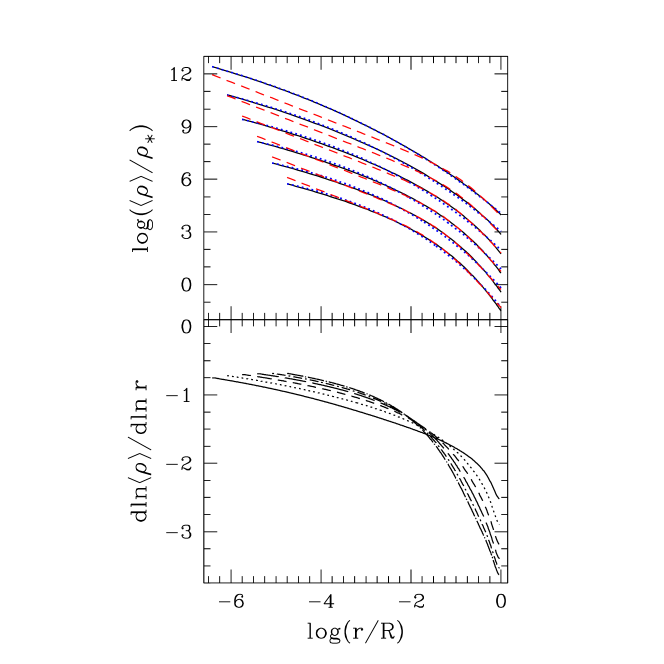
Figure 1: Predicted density profiles (top panel) as a function of radial distance in units of virial radius, R, for halos at $z=0$ (black solid lines), compared to their best fit by a NFW law (red dashed lines) and by a Sérsic law (blue dotted lines) down to R/100 and 1 pc, respectively, for halos with $10^{10}$, $10^{11}$, $10^{12}$, $10^{13}$, $10^{14}$ and $10^{15}$ M_⊙ (from bottom to top). The normalization constant $\rho_{\ast}$ is defined as $\bar{\rho}M_{\ast}/M$ where $M_{\ast}=10^{13}$ M_⊙ is the critical mass for collapse. Corresponding radial dependence of logarithmic slopes (bottom panel) for the same halo masses: $10^{10}$ M_⊙ (dot-long dashed line), $10^{11}$ M_⊙ (dot-short dashed line), $10^{12}$ M_⊙ (long dashed line), $10^{13}$ M_⊙ (short dashed line), $10^{14}$ M_⊙ (dotted line) and $10^{15}$ M_⊙ (solid line).

3 TYPICAL PROFILES

The fact that all the preceding profiles are unique for given current values of the corresponding accretion rates is not of much help, in general, for inferring them for any particular halo. This requires performing the analytical extension of the respective small pieces developed by accretion in any finite time interval, which is not an easy task. However, what can be readily derived in the way explained next is the typical radial behavior of all these profiles.

3.1 Density Profile

As noted by SMGH, the analytical extension of the typical mass profile $M(r)$ is simply the transformation from $t$ to $r$ through the inverse of equation (20) of the analytical $M(t)$ track solution of the differential equation

$$\frac{\dot{M}}{M(t)}={\cal R}_{\rm a}[M(t),t]\,,$$ (27)

where

$${\cal R}_{\rm a}[M(t),t]=\int_{0}^{M\Delta_{\rm m}}\!\!\!{\rm d}(\Delta M)\;\Delta M\;{\cal R}_{\rm m}(M,t,\Delta M)\,$$ (28)

is the analytical typical scaled accretion rate in the cosmology under consideration (Raig et al. 2001). Then, one must simply differentiate such a mass profile to obtain the desired typical density profile,

$$\langle\rho\rangle(t)=\Delta_{\rm vir}(t)\bar{\rho}(t)~{}~{}~{}~{}~{}~{}~{}~{}~{}~{}~{}~{}~{}~{}~{}~{}~{}~{}~{}~{}~{}~{}~{}~{}~{}~{}~{}~{}~{}$$

$$\times\,\left[1-\frac{1}{{\cal R}_{\rm a}[M(t),t]}\;\frac{{\rm d}\ln(\Delta_{\rm vir}\bar{\rho})}{{\rm d}t}\right]^{-1}\,,$$ (29)

for $t(r)$ equal to the inverse of $R(t)$ given by equation (20). In equation (28), ${\cal R}_{\rm m}(M,t,\Delta M)$ is the usual merger rate in the extended Press-Schechter (PS) formalism (Lacey & Cole 1993) and the integral extends only over those mergers producing a relative mass increase below the effective ratio $\Delta_{\rm m}=\Delta M/M$ separating minor from major mergers as the former are the only ones to contribute accretion. As shown in SMGH, the best effective value of this threshold, equal to 0.26, gives an excellent fit to the empirical NFW $c(M)$ relation over at least 4 decades in halo mass (see Fig. 2 in SMGH).

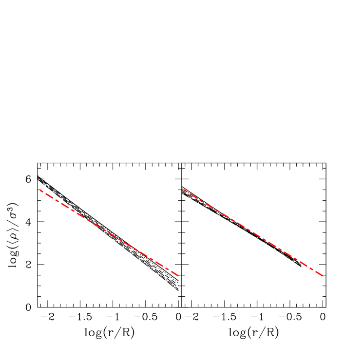
Figure 2: Predicted phase-space density profiles at $z=0$ for the same halo masses as in Figure 1 (and same symbols as in the bottom panel of that figure). The red thick long dashed-short dashed line is the empirical curve obtained by Ascasibar et al. (2004). Left panel: predictions obtained from the spherical collapse model without shell-crossing. Right panel: predictions obtained from the phenomenological correction for shell-crossing with $\eta=1.8$. The density and velocity dispersion are in units of the cosmic critical density and of halo circular velocity, respectively.

Figure 3: Predicted phase-space density profile for a halo of $10^{13}$ M_⊙ at $z=0$ for different values of $\eta$: $0$ (long dashed line), $1$ (dot-dashed line) $1.5$ (short dashed line), $1.8$ (solid line) and $2$ (dotted line) compared to the empirical curve obtained by Ascasibar et al. (2004) (red thick long dashed-short dashed line).

In the top panel of Figure 1 we show the predicted density profiles, for $\Delta_{\rm m}=0.26$, corresponding to various halo masses at $z=0$, compared to their respective best fits down to a radius of one hundredth $R$ and 1 pc by a NFW law (eq. [1]) and an Einasto law (eq. [2]), respectively. As mentioned, not only is the density profile well fit by an NFW law down to one hundredth the virial radius as found in numerical simulations, but the mass-concentration relation is also perfectly recovered. In respect to the fit by an Einasto law, there is so far no accurate mass dependence of the corresponding parameters in the literature; see SMGH for that predicted by the present model. In the bottom panel of Figure 1 we plot the corresponding logarithmic slopes as a function of radius, where the tendency to approach, at small radii, the functionality ${\rm d}\ln\langle\rho\rangle/{\rm d}\ln r\propto-r^{1/n}$ characteristic of the Einasto law is more apparent.

3.2 Velocity Dispersion Profile

To derive the typical $\sigma$ profile we need to know the typical energy accretion rate $\dot{E}$ going along with the typical mass accretion rate $\dot{M}$ given above. Although there is no expression similar to (27) for $\dot{E}$, we can try to estimate it by means of conservation arguments from the typical total energy of the halo seeds at any arbitrarily small time $t_{\rm i}$.

When the total mass $M(t)$ of virialized objects at $t$ is to be estimated it is very useful to approximate protohalos by smooth spherical top-hat perturbations. This does not work however when dealing with the total energy $E(t)$ because it depends on the halo mass and velocity distributions at all scales. (Nor does it help taking into account that protohalos would coincide with peaks of the smoothed density field.) Determining accurately the total energy of the protohalo is, in general, a very difficult task. But, in the present case, we can take advantage of the fact that the structure and kinematics of the final halo do not depend on its past aggregation history and adopt the point of view that it has evolved since $t_{\rm i}$ by pure accretion. That assumption and the neglect of triaxiality effects as done in the Appendix for the final relaxed halos allow one to deal with those seeds as if they were spherically symmetric.

In this case, the radius $R_{\rm ph}$ of that part of the protohalo collapsing at $t$ is

$$R_{\rm ph}^{3}(t)=\frac{3M(t)}{4\pi\bar{\rho}(t_{\rm i})[1+\delta(t,t_{\rm i})]}\,,$$ (30)

where $\delta(t,t_{\rm i})=\delta_{\rm c}D(t_{\rm i})/D(t)$ is the density contrast for spherical collapse at $t$, with $\delta_{\rm c}$ the critical value for current collapse (equal to 1.69 in any flat cosmology) and $D(t)$ the perturbation linear growth factor. Consequently, its mass and total energy (for the system truncated at $R_{\rm ph}$ and with potential origin at infinity) are

$$M(t)=4\pi\int^{R_{\rm ph}(t)}_{0}{\rm d}r\;r^{2}\;\rho_{\rm ph}(r)$$ (31)

$$E(t)=4\pi\!\!\int^{R_{\rm ph}(t)}_{0}\!\!{\rm d}r\,r^{2}\rho_{\rm ph}(r)\!\left[\frac{u^{2}_{\rm ph}(r)}{2}\!-\!\frac{GM_{\rm ph}(r)}{r}\right]\!\!,$$ (32)

where $\rho_{\rm ph}(r)$ and $M_{\rm ph}(r)$ are the exact, spherically averaged, density and mass profiles, respectively, of the protohalo and $u_{\rm ph}(r)$ is the velocity of the shell at $r$, essentially equal to the Hubble component, $H(t_{\rm i})r$. Differentiating over $R_{\rm ph}(t)$ both $M(t)$ and $E(t)$, respectively given by equations (31) and (32), and substituting these derivatives into equation (22), one is led, after some algebra and to leading order in the perturbation $\delta(t,t_{\rm i})$, to

$$\sigma^{2}(t)=2\frac{GM(t)}{R(t)}\left[1-\frac{\delta_{\rm c}}{\Delta_{\rm vir}^{1/3}(t)}\right]\,,$$ (33)

yielding, for $t$ equal to the inverse of $R(t)$, the wanted typical $\sigma^{2}(r)$ profile. Equation (33) coincides with the expression we would have obtained from the usual top-hat approximation, so the detailed density and velocity distributions in the protohalo do not actually play any role in the final result. The reason for this is that the specific density profile $\rho_{\rm ph}(r)$ cancels when taking the ratio between the time derivatives of $E$ and $M$ in equation (22). This is the consequence of the fact that, as the velocity dispersion profile is developing inside-out, its value at $r$ depends only on the specific energy of the protohalo at the corresponding radius, not on its total inner value.

The phase-space density profile $\langle\rho\rangle/\sigma^{3}$ arising from such a velocity dispersion profile and the spherically averaged density profile derived in Section 3.1 is shown in the left panel of Figure 2. For comparison, we plot the empirical best-fitting power law of index $\nu=1.9$ obtained by Ascasibar et al. (2004). The theoretical prediction agrees with the result of numerical simulations (despite the lack of any free parameter to adjust) not only in its overall shape, close to a power law over more than five decades in halo mass, but also in its magnitude. The only small discrepancy is that the predicted profile is somewhat steeper than empirically found ($\nu\sim 2.3$ instead of $1.9$). This is most likely due to the fact that we have neglected shell-crossing.

Shell-crossing brakes the infall of collapsing matter, so the bulk velocity of deep enough layers is much smaller than predicted by the top-hat collapse model without shell-crossing. In fact, the system is essentially steady within the virial radius $R$ (Cole & Lacey 1996). Unfortunately, shell-crossing cannot be dealt with analytically, so the mass within $R(t)$ can only be estimated phenomenologically from the predictions of that simple collapse model. Next a similar approach is used to estimate the total energy of the object within $R(t)$.

The mass within the shell of the protohalo at $R_{\rm ph}$ having an inner mean density contrast appropriate for collapse, without shell-crossing, at $t$ appears to coincide with the mass $M$ of the final steady object within the virial radius $R$, defined through equation (20), at that moment. This does not mean, of course, that the particles inside $R$ coincide with those initially located inside $R_{\rm ph}$. Some have rebound and are currently beyond $R(t)$, while others initially beyond $R_{\rm ph}$ have already passed by $R(t)$. Yet, as far as the mass within $R(t)$ coincides with that of the protohalo within $R_{\rm ph}$, the mass of these two kinds of particles balance each other and we must not worry about that distinction. However, the situation is different when dealing with total energy. Particles having bounced were originally more tightly bound than those having not yet. Thus, the total energy within $R(t)$ is larger than estimated through equation (32) (kinetic energy transfer among shells through two-body interactions at shell crossing is negligible). In other words, it is given by that equation at a larger time and the same result holds for the velocity dispersion at $R$: it is given by equation (33) at some later time $t+\Delta t$. Inspired of the fact that the shift $\Delta t$ in the case of $M(t)$ is null for all halo masses and cosmologies, a reasonable guess for the shift $\Delta t$ in the case of energies is to assume it equal to $\eta t$ with $\eta$ equal to the same positive constant factor for all halo masses and cosmologies. This leads to (see eq. [33])

$$\sigma^{2}(t)=2\frac{GM[(1+\eta)t]}{R[(1+\eta)t]}\left\{1-\frac{\delta_{\rm c}}{\Delta_{\rm vir}^{1/3}[(1+\eta)t]}\right\}\,.$$ (34)

Moreover, since the shift $\eta t$ is caused by shell-crossing and the characteristic bounce time of shells that would collapse at $t$ if there were no shell-crossing is equal to $t$, we expect an $\eta$ value of order unity.

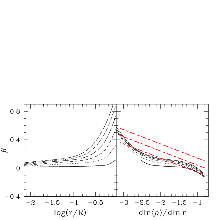
Figure 4: Predicted anisotropy profile as a function of radius (left panel) or density logarithmic slope (right panel) obtained for the same halo masses as in Figure 2. For comparison, we plot the best linear fit to empirical data on this latter relation drawn from numerical simulations (central red thick short dashed-long dashed line) and its scatter (bracketing red thick lines). For $r$ tending to zero, the predicted anisotropy tends to become negative. Whether this is a real effect or a numerical artifact (caused, e.g., by the extrapolation of our phenomenological correction for shell crossing down to $r=0$) is hard to tell at this stage.

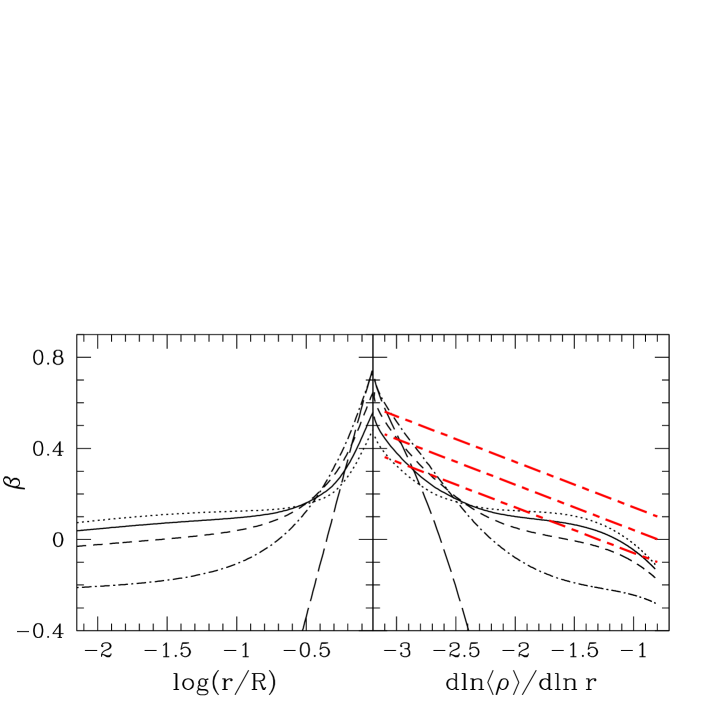
Figure 5: Same as Figure 3 for the predicted anisotropy profile, showing the effect of the phenomenological factor $\eta$. Full line ($\eta=1.8$) gave a good fit when comparing the theoretical $\langle\rho\rangle/\sigma^{3}$ to those of simulations, and it is also seen to provide a reasonable fit to $\beta$.

In the right panel of Figure 2, we depict the phase-space density profile arising from the spatial velocity dispersion given in equation (34) for $t(r)$ equal to the inverse of $R(t)$ and $\eta=1.8$. As can be seen, this new $\sigma$ profile is in much better agreement, indeed, with the results of simulations.

To see the effect of varying $\eta$, we show, in Figure 3, the profiles resulting from different values of that parameter. For any value of $\eta$ greater then zero, the solution $\sigma(r)$ at large enough radii relies on the extrapolation towards the future of the Bryan and Norman (1998) expression for $\Delta_{\rm vir}$. For $\eta=1.8$, this affects the solutions at radii above $\log(r/R)\sim-0.35$ for all halo masses (see Figs. 2 and 3 where all profiles are plotted only for smaller radii). As such an extrapolation is quite uncertain, from now on, the corrected $\sigma$ profile at such large radii is inferred from the much more secure linear extrapolation of the predicted phase-space density profile.

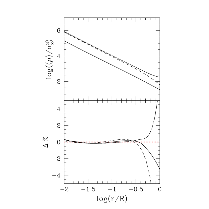
Figure 6: Top panel: predicted phase-space densities for a halo of $10^{13}$ M_⊙ at $z=0$ corresponding to the radial ($\sigma_{\rm x}\equiv\sigma_{\rm r}$, dashed line), tangential ($\sigma_{\rm x}\equiv\sigma_{\rm t}$, dot-dashed line) and spatial ($\sigma_{\rm x}\equiv\sigma$, solid line) velocity dispersions obtained with $\eta=1.8$ as in the right panel of Figure 2. Bottom panel: residuals from the respective fit to a power-law of the form $Ar^{-\nu}$ with best-fitting exponents equal to $1.89$ (spatial case), $1.92$ (radial case) and $1.87$ (tangential case); all fits achieved in the radial range requiring no extrapolation.

Figure 7: Mass dependence of the power index $\nu$ (top panel) and the proportionality factor $A$ (bottom panel) of the best-fitting power law $Ar^{-\nu}$ for the predicted spatial, radial and tangential phase-space densities (same symbols as in Fig. 6).

3.3 Anisotropy Profile

After a change of integration variable, the approximate relation (24) takes the form

$$\sigma^{2}_{\rm r}(t)=\frac{1}{4\pi R^{3}(t)\,\langle\rho\rangle(t)}~{}~{}~{}~{}~{}~{}~{}~{}~{}~{}~{}~{}~{}~{}~{}~{}~{}~{}~{}~{}~{}~{}~{}~{}~{}~{}~{}$$

$$\!\times\!\!\int_{0}^{t}\!\!{\rm d}\tilde{t}\left[\sigma^{2}(\tilde{t})-\frac{GM(\tilde{t})}{R(\tilde{t})}\right]\!{\cal R}_{\rm a}[M(\tilde{t}),\tilde{t}]\,M(\tilde{t}),~{}$$ (35)

leading, for $t(r)$ equal to the inverse of $R(t)$, to the (approximate) typical radial velocity dispersion profile and, through equation (4), to the (approximate) typical $\beta(r)$ profile. Note that, as $\sigma$ was derived to leading order in the perturbation $\delta$ at $t_{\rm i}$, its central behavior is not fully reliable, so is not either that of the $\sigma_{\rm r}$ profile. However, the behavior at moderate and large radii of $\sigma_{\rm r}(r)$ is quite robust because the integral appearing in equation (35) is very insensitive to the central values of $\sigma$.

In the left panel of Figure 4, we plot the predicted typical $\beta(r)$ profile for the same current halos and the same radii as in Figure 2. In the right panel, we show the corresponding relation between $\beta$ and the logarithmic slope of the density profile. The theoretical anisotropy shows a trend similar to that empirically found by Hansen & Moore (2006), although with some apparent undulations. Similar variations have recently been observed in numerical experiments (McMillan et al. 2007). Whether these undulations are real or an artifact due to the approximate character of our solution is hard to tell. Note that the rough universality of the $\beta$ profile combined with the fact that the typical halo density profile at $t$ depends only on the halo mass leads to the conclusion that the typical anisotropy profile depends essentially only on the halo mass, too.

Of course, such a predicted typical anisotropy profile depends on the exact value of $\eta$ chosen to correct the theoretical velocity dispersion profile for the effects of shell-crossing. To see more quantitatively the influence of such a correction, we plot in Figure 5 the solutions arising from the different values of $\eta$ used in Figure 3.

Once we have determined the typical radial and tangential velocity dispersion profiles we can check if the corresponding phase-space density profiles are again close to power laws. The result is shown in Figure 6 where we also plot the residuals of each profile from the corresponding best fit by a power-law in $r$ (eq. [3]). As can be seen, the phase-space density profiles for the radial and tangential velocity dispersions also admit a power law fit like that associated with the spatial velocity dispersion with similar values of index $\nu$ and just a small shift in the respective proportionality factors, in agreement with the results of numerical simulations (Ascasibar et al 2004; Dehnen & McLaughlin 2005). Among these two profiles that associated with the tangential dispersion, $\langle\rho\rangle/\sigma^{3}_{\rm t}$, is the one giving the best fit to a power-law in radius (in the range requiring no extrapolation), with a slope $\nu\sim 1.9$. This result is most likely related to the fact that the tangential velocity distribution function has virtually the same shape for all radii (Hansen et al. 2006). This is contrasted with the radial velocity distribution function, whose shape changes significantly as function of radius.

In Figure 7 we show the mass dependence of the best fitting parameters $\nu$ and $A$ to all three phase-space density profiles.

3.4 Angular Momentum Profile

Equations (26) and (27) define, for $t(r)$ equal to the inverse of $R(t)$, the $\langle j\rangle(r)$ profile in terms of $\dot{J}$, which can be computed from equation (6) or (7), assuming typical values for both the spin parameter and its time derivative.

As mentioned, the mean spin values and standard deviations are found in $N$-body simulations to be quite insensitive to the cosmology, halo mass and particular epoch considered. When looking at their behavior in more detail, it is observed however that, just after major mergers, they take values substantially higher than the mean (Burkert & D’Onghia 2004), which is likely due to the fact that halos are not yet fully relaxed. What is more important for our purposes here, $\lambda^{\prime}$ depends on halo mass according to equation (8) (B01b), its mean value being essentially constant while the mean $\lambda$ value is essentially independent of mass (B01b) and shows a slight secular evolution (Hetznecker and Burkert 2006). This latter result is found regardless of whether the means are performed over all the halos or just accreting ones. According to the relation (8), the spin parameters of a given accreting halo satisfy the relation

$$\lambda^{\prime}(t)=\lambda(t)F\{c[M(t),t]\}\,.$$ (36)

Taking the mean of this latter equation over halo masses in the relevant mass range at $t$ and taking into account that the mean $\lambda^{\prime}$ is constant and equal to 0.039 , one is led to

$$\lambda(t)=\frac{0.039}{\bar{F}(t)}\,.$$ (37)

where $\bar{F}(t)$ stands for the mean of $F[c(M,t)]$ with $F(c)$ given by equation (9) and $c(M,t)$ the NFW mass-concentration relation at $t$ given in SMGH (see their eq. [10]). Note that, at present, $c$ is around $10$ for masses in the relevant range (between $10^{10}$ M_⊙ and $10^{15}$ M_⊙), so $\bar{F}$ is about unity. We have checked that the time-dependence of the mean $\lambda$ value implied by the approximate relations (36)–(37) is also a reasonable approximation of the one found by Hetznecker and Burkert (2006).

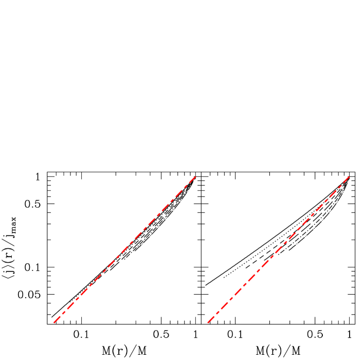
Figure 8: Predicted specific angular momentum profile for the same halo masses (marked with identical symbols) as in Figures 2 and 4 derived using the $\lambda$ (left panel) and $\lambda^{\prime}$ (right panel) spin parameters. For comparison, we plot the average power law with $s=1.3$ fitting, to a first approximation, numerical data according to B01b (red thick short dashed-long dashed line).

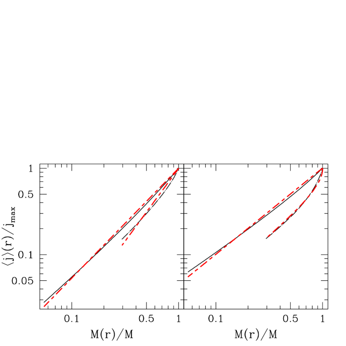
Figure 9: Same predicted specific angular momentum profiles (and same symbols) as in Figure 8, and the corresponding fits either by a power law for the $\lambda$ case (left panel), or by the slight modification of it given in the text for the $\lambda^{\prime}$ case (right panel). To avoid overcrowding, we only represent the curves corresponding to $10^{10}$ M_⊙ and $10^{15}$ M_⊙.

Differentiating equations (6) and (7), we obtain the typical angular momentum accretion rate

$$\frac{\dot{J}}{J(t)}=\frac{\dot{M}}{M(t)}\Biggl{\{}\frac{5}{2}-\frac{1}{{\cal R}_{\rm a}[M(t),t]}\left[\frac{\dot{E}}{2E(t)}-\frac{\dot{\lambda}}{\lambda(t)}\right]\Biggr{\}}$$ (38)

and

$$\frac{\dot{J}}{J(t)}=\frac{\dot{M}}{M(t)}\Biggl{\{}\frac{5}{3}-\frac{1}{{\cal R}_{\rm a}[M(t),t]}~{}~{}~{}~{}~{}~{}~{}~{}~{}~{}~{}~{}~{}~{}~{}~{}~{}$$

$$\times\,\left[\frac{{\rm d}\ln(\Delta_{\rm vir}\bar{\rho})^{1/6}}{{\rm d}t}-\frac{\dot{\lambda}^{\prime}}{\lambda^{\prime}(t)}\right]\Biggr{\}}\,,$$ (39)

respectively. In equation (38), the energy accretion rate $\dot{E}$ is computed from equation (23), with $\sigma(t)$ according to the expression (34) and $\langle\Phi\rangle$ the spherically averaged gravitational potential at $R$ of the halo endowed with a NFW profile up to infinity, and $E(t)$ is obtained by integrating $\dot{E}$ over time. In deriving equation (39) from equation (7), we have taken into account the definition of the virial radius (eq. [20]) and the expression of $\langle\rho\rangle(t)$ given by equation (29). Note that the expression (39) making use of $\lambda^{\prime}$ does not depend neither on the phenomenological correction for shell-crossing of the $\sigma$ profile nor on the assumed mass distribution beyond $R(t)$.

By substituting into equation (26) the previous expressions for $\dot{J}$ and taking into account the typical values of the spin parameters given by expressions (36) and (37), we are finally led to the two following, in principle equivalent, estimates of the typical spherically symmetric specific angular momentum profile,

$$\langle j\rangle(t)=\frac{J(t)}{M(t)}\Biggl{\{}\frac{5}{2}-\frac{1}{{\cal R}_{\rm a}[M(t),t]}\left[\frac{\dot{E}}{2E(t)}-\frac{\dot{\lambda}}{\lambda(t)}\right]\Biggr{\}}$$ (40)

and

$$\langle j\rangle(t)=\frac{J(t)}{M(t)}\Biggl{\{}\frac{5}{3}-\frac{1}{{\cal R}_{\rm a}[M(t),t]}~{}~{}~{}~{}~{}~{}~{}~{}~{}~{}~{}~{}~{}~{}~{}~{}~{}$$

$$\times\,\left[\frac{{\rm d}\ln(\Delta_{\rm vir}\bar{\rho})^{1/6}}{{\rm d}t}-\frac{\dot{\lambda}^{\prime}}{\lambda^{\prime}(t)}\right]\Biggr{\}}\,,~{}~{}$$ (41)

for $t(r)$ equal to the inverse of $R(t)$ and $J(t)$ the total angular momentum accretion track, given by equations (6) or (7) for the appropriate values of $M(t)$, $E(t)$ and $\lambda(t)$ or $\lambda^{\prime}(t)$.

These two estimates of the angular momentum profile are shown in Figure 8. As can be seen, the solutions derived from $\lambda$ and $\lambda^{\prime}$ are slightly different from each other. This cannot be due to the value of $\eta$ used to infer the solution from $\lambda$ because, as shown in Figure 10, the solutions appear to be remarkably insensitive, in this occasion, to the value of that parameter. We have also checked that the extrapolation of the density profile beyond $R$ has a very small effect. Thus, it can only be due to the time dependence adopted for $\lambda$ and $\lambda^{\prime}$. In fact, the information we have on the empirical behavior of the spin parameters refers only to redshifts smaller than 2 (see Hetznecker and Burkert 2006). For this reason, in Figure 8, the predicted solutions are only drawn for radii involving $z\leq 5$.

Anyhow, both solutions show similar trends in agreement with the results of numerical simulations. They are indeed power laws in mass inside $r$ to a first approximation, particularly the solution obtained from $\lambda$, with a mean best-fitting value of index $s$ (with the restriction $\langle j\rangle(R)/j_{\rm max}=1$) close to that found empirically. More specifically, for the masses included in our figures and a PS mass distribution, we obtain (within the radial range plotted in Fig. 8 for each mass) $\bar{s}\sim 1.6$ and $\sim 1.7$ for the $\lambda$ and $\lambda^{\prime}$ cases, respectively. While for the mass interval studied by B01b ($>10^{12}$ M_⊙) we obtain $\bar{s}\sim 1.3$ and $\sim 1.4$ to be compared with the value of $\sim 1.3$ quoted by these authors. Furthermore, the slight bending upwards at large radii, more apparent in the $\lambda^{\prime}$ case although also present in the $\lambda$ one as all the curves must approach unity at $r=R$, is also observed in simulated halos (see the comments in B01b). Finally, the tendency for less massive halos to have slightly steeper profiles (in the mean all over the radial range analyzed) is also consistent with the empirical results of B01b (see their Fig. 16).

As a power law does not seem to give a very good fit to the solutions drawn from $\lambda^{\prime}$ we have tried with another simple analytical expression. As shown in Figure 9, the following slight modification

$$\frac{\langle j\rangle(r)}{j_{\rm max}}=1-\left[1-\frac{M(r)}{M(R)}\right]^{s^{\prime}},$$ (42)

is already enough to improve notably the fits for all halo masses. Note that the solutions drawn from $\lambda$ are however better fit by the previous simple power law of index $s$. The dependence on $M$ of that index $s$ and the new one $s^{\prime}$ is given in Figure 11 for the solutions drawn from $\lambda$ and $\lambda^{\prime}$, respectively.

Figure 10: Same as Figures 5 and 3 but for the angular momentum profile predicted using $\lambda$ for the extreme cases of $10^{10}$ M_⊙ (lower curves) and $10^{15}$ M_⊙ (upper curves) in order to show the degree of insensitivity to parameter $\eta$ for solutions corresponding to different halo masses.

Figure 11: Mass dependence of the best fitting parameters $s$ and $s^{\prime}$ in the power law and the modification of it proposed to fit the specific angular momentum profile drawn from $\lambda$ (solid line) and $\lambda^{\prime}$ (dashed line), respectively.

4 SUMMARY AND CONCLUSIONS

We consider the structural and kinematic properties of realistic ellipsoidal, rotating, standard CDM halos in the accretion-driven scenario. According to this scenario, halos adapt dynamically to the amount of matter (carrying mass, energy and angular momentum) that is accreted at any given moment. This is due to the collisionless nature of CDM and the inside-out growth of these structures during accretion phases. The typical accretion rate for halos of a given mass at a given cosmic time depends only on the cosmology, and thus, the typical radial profiles of relaxed dark matter halos are fixed by cosmological parameters.

Specifically, we derive the typical spherically averaged profiles corresponding to the density $\rho$, the velocity dispersion $\sigma$ and the phase-space density $\rho/\sigma^{3}$. We find that all these predicted profiles are in good agreement with those found in numerical simulations. In particular, $\rho$ is well fit, in 3D, by an Einasto function and $\rho/\sigma^{3}$ by a power law, $Ar^{-\nu}$, with $\nu\approx 1.9$ and $\log A\approx 1.4$.

We also derive the typical profile of the velocity anisotropy $\beta$. We find that the anisotropy increases from something small (maybe slightly negative) at the halo center to a positive value in the outer region and with a typical logarithmic slope also in agreement with numerical data. This is the first time that a non-zero anisotropy has been derived from first principles. We find that the spherically averaged phase-space density associated to the tangential (radial) velocity dispersion, $\rho/\sigma_{\rm t}^{3}$ ($\rho/\sigma_{\rm r}^{3}$) is also close to a power law with slope $\nu\approx 1.9$ although somewhat different values of $A$.

We finally derive the typical spherically averaged profile of the specific angular momentum $j$ from the empirical evolution of the dimensionless halo spin parameter $\lambda$ or $\lambda^{\prime}$. We find that this profile scales, to a first approximation, as a power law in inner mass, $j(r)\propto[M(r)]^{s}$, in agreement with numerical simulations. The average logarithmic slope $s$ found using $\lambda$ coincides with the empirical value of 1.3, while that found using $\lambda^{\prime}$ (1.4) is also close to it. A more accurate analytical expression is provided for the $j(r)$ profile derived from $\lambda^{\prime}$.

We find that all the preceding profiles depend moderately on halo mass. The dependence of the NFW and Einasto parameters fitting the density profile in any given cosmology were already presented in SMGH. Here we have focused on the mass dependence of the remaining profiles. The behavior of any of these profiles found in observations (for instance, the logarithmic slope of the density profile obtained from X-rays or strong gravitational lensing) could in principle be used, in a given cosmology, to estimate the total mass of the system. Since the total mass most often is known, this also provides a direct way of observationally testing the predictions of this accretion driven scenario.

The anisotropy and velocity dispersion (or phase-space density) profiles are derived using a practical phenomenological correction for the effects of the complex process of shell-crossing on the total energy of halos conserved since the epoch they were density perturbations. This correction is achieved by adjusting the value of one free parameter, $\eta$. We find that both the anisotropy profile and the phase-space density profile are in good agreement with numerical results for $\eta\approx 1.8$, the angular momentum profile being instead insensitive to the value of this parameter.

The fact that all our results are in fairly good agreement with those drawn from numerical cosmological simulations leads support to the idea that the structural and kinematic properties of dark matter structures are determined by their dynamical adaption to cosmological accretion.

Appendix A JEANS EQUATION AND SCALAR VIRIAL RELATION

A.1 Exact Relations

The internal dynamics of relaxed inside-out evolving halos should be well-described by a steady (true) phase-space density $f({\mathbf{r}},{\mathbf{v}})$ satisfying the collisionless Boltzmann equation. Writing this equation in spherical coordinates (see, e.g., equation [4p-2] of Binney & Tremaine 1987), multiplying it by the radial velocity $v_{\rm r}$, and integrating over velocity and solid angle, one is led to the following first order differential equation

$$\frac{{\rm d}(\langle\rho\rangle\sigma_{\rm r}^{2})}{{\rm d}r}+\frac{\langle\rho\rangle(r)}{r}(3\sigma_{\rm r}^{2}(r)-\sigma^{2}(r))=-\frac{1}{4\pi}\int_{0}^{2\pi}\!\!{\rm d}\varphi\!\int_{0}^{\pi}\!\!{\rm d}\theta\;\sin\theta\;{\rho\,\partial_{\rm r}\Phi}\,,$$ (A1)

where $\sigma$ stands for the non-centered velocity dispersion in the shell at $r$,

$$\sigma^{2}(r)=\frac{1}{4\pi\langle\rho\rangle}\int_{0}^{2\pi}\!\!{\rm d}\varphi\!\int_{0}^{\pi}\!\!{\rm d}\theta\;\sin\theta\;{\int{\rm d}^{3}v\,v^{2}\,f}=\sigma^{2}_{\rm r}(r)+\sigma^{2}_{\theta}(r)+\sigma^{2}_{\varphi}(r)\,,$$ (A2)

$\langle\rho\rangle$ for the spherically averaged density profile of the halo given by equation (12), with the local density distribution satisfying the relation

$$\rho(r,\theta,\varphi)=\int{\rm d}^{3}v\,f({\mathbf{r}},{\mathbf{v}})\,,$$ (A3)

and $\partial_{\rm r}$ for the radial partial derivative. To derive equation (A1), it is only needed such conventional assumptions as the continuity, in real space, of the local density and mean velocities and the fact that $f$ vanishes for large velocities. In expression (A1), we have taken into account that the effects of a non-null cosmological constant are negligible on halo scales.

Splitting the local density and gravitational potential as

$$\rho(r,\theta,\varphi) = \langle\rho\rangle(r)+\delta\rho(r,\theta,\varphi)$$ (A4)

$$\Phi(r,\theta,\varphi) = \langle\Phi\rangle(r)+\delta\Phi(r,\theta,\varphi)\,,$$ (A5)

and taking into account that the spherically averaged gravitational potential,

$$\langle\Phi\rangle(r)=\frac{1}{4\pi}\int_{0}^{2\pi}\!\!{\rm d}\varphi\!\int_{0}^{\pi}\!\!{\rm d}\theta\;\sin\theta\;{\Phi(r,\theta,\varphi)},$$ (A6)

satisfies, by the Gauss theorem, the usual relation for spherically symmetric systems

$$\frac{{\rm d}\langle\Phi\rangle(r)}{{\rm d}r}=\frac{GM(r)}{r^{2}},$$ (A7)

equation (A1) adopts the form

$$\frac{{\rm d}(\langle\rho\rangle\sigma_{\rm r}^{2})}{{\rm d}r}+\frac{\langle\rho\rangle}{r}(3\sigma_{\rm r}^{2}-\sigma^{2})=-\langle\rho\rangle\frac{GM(r)}{r^{2}}-\frac{1}{4\pi}\int_{0}^{2\pi}\!\!{\rm d}\varphi\!\int_{0}^{\pi}\!\!{\rm d}\theta\;\sin\theta\;{\delta\rho\,\partial_{\rm r}(\delta\Phi)}\,.$$ (A8)

Except for the second term on the right, equation (A8) looks exactly as the classical Jeans equation for spherically symmetric systems with anisotropic velocity tensor. Thus, multiplying (A8) by $4\pi r^{3}{\rm d}r$ and integrating over $r$, the same steps leading to the scalar virial relation for a spherically symmetric system now lead to

$$4\pi R^{3}P(R)-2K=-\int_{0}^{R}{\rm d}M(r)\frac{GM(r)}{r}-\int_{0}^{R}{\rm d}r\,r^{3}\int_{0}^{2\pi}\!\!{\rm d}\varphi\!\int_{0}^{\pi}\!\!{\rm d}\theta\;\sin\theta\;{\delta\rho\,\partial_{\rm r}(\delta\Phi)}\,,$$ (A9)

where ${\rm d}M(r)=4\pi r^{2}\langle\rho\rangle(r){\rm d}r$ is the mass of the elementary spherical shell of radius $r$,

$$P(R)=\langle\rho\rangle(R)\sigma_{\rm r}^{2}(R)$$ (A10)

is the spherically averaged radial boundary pressure, and

$$K=\frac{1}{2}\int_{0}^{R}{\rm d}M(r)\sigma^{2}(r)$$ (A11)

is the kinetic energy within $R$.

On the other hand, the total potential energy is

$$W=\frac{1}{2}\int_{0}^{R}{\rm d}r\,r^{2}\int_{0}^{2\pi}\!\!{\rm d}\varphi\!\int_{0}^{\pi}\!\!{\rm d}\theta\;\sin\theta\;{\rho(r,\theta,\varphi)\,\Phi(r,\theta,\varphi)}\,,$$ (A12)

which, from equations (A4)–(A5), can be written as

$$W=2\pi\int_{0}^{R}{\rm d}r\,r^{2}\langle\rho\rangle(r)\,\langle\Phi\rangle(r)+\frac{1}{2}\int_{0}^{R}{\rm d}r\,r^{2}\int_{0}^{2\pi}\!\!{\rm d}\varphi\!\int_{0}^{\pi}\!\!{\rm d}\theta\;\sin\theta\;{\delta\rho\,\delta\Phi}\,.$$ (A13)

Provided the central asymptotic logarithmic slope of $\langle\rho\rangle$ is greater than $-5/2$, fixing the origin of the potential $\Phi$ so to have the boundary condition

$$\langle\Phi\rangle(R)=-\frac{GM}{R}\,,$$ (A14)

for the differential equation (A7) (this is essentially equivalent to consider the potential origin at infinity for the system truncated at $R$) and integrating by parts (two consecutive times) the first term on the right of equation (A13), the potential energy takes the form

$$W=-\int_{0}^{R}{\rm d}M(r)\,\frac{GM(r)}{r}+\frac{1}{2}\int_{0}^{R}{\rm d}r\,r^{2}\int_{0}^{2\pi}\!\!{\rm d}\varphi\!\int_{0}^{\pi}\!\!{\rm d}\theta\;\sin\theta\;{\delta\rho\,\delta\Phi}\,.$$ (A15)

Therefore, by subtracting $2W$ on both sides of equation (A9) we arrive to the virial relation

$$4\pi R^{3}P(R)-2E=\int_{0}^{R}{\rm d}M(r)\,\frac{GM(r)}{r}-\int_{0}^{R}\!{\rm d}r\,r^{2}\!\int_{0}^{2\pi}\!\!{\rm d}\varphi\!\int_{0}^{\pi}\!\!{\rm d}\theta\;\sin\theta\;{\delta\rho\,\left[\delta\Phi+r\partial_{\rm r}(\delta\Phi)\right]}\,.$$ (A16)

where the total energy $E=K+W$ is given by

$$E=\int_{0}^{R}{\rm d}M(r)\,\left[\frac{\sigma^{2}}{2}-\frac{GM(r)}{r}\right]+\frac{1}{2}\int_{0}^{R}{\rm d}r\,r^{2}\int_{0}^{2\pi}\!\!{\rm d}\varphi\!\int_{0}^{\pi}\!\!{\rm d}\theta\;\sin\theta\;{\delta\rho\,\delta\Phi}\,.$$ (A17)

A.2 Approximate Relations

Although halos exhibit substantial triaxiality (the average minor to major axial ratio takes a value between $0.6$ and $0.7$; Bullock 2002, Kasun & Evrard 2005, Bailin & Steinmetz 2005, Libeskind et al. 2005), their mass distribution is far from flattened and the isopotential surfaces are more spherical (cf. Binney & Tremaine 1987). We therefore have

$$\frac{|\delta\rho|}{\langle\rho\rangle} < 1$$ (A18)

$$\frac{|\delta\Phi|}{|\langle\Phi\rangle|} \ll 1\,.$$ (A19)

Moreover, since the isopotential surfaces approach to spheres as $r$ increases, the rms value of $\delta\Phi$ in the spherical shell at $r$,

$$\sigma_{\Phi}(r)=\left[\frac{1}{4\pi}\int_{0}^{2\pi}\!\!{\rm d}\varphi\!\int_{0}^{\pi}\!\!{\rm d}\theta\;\sin\theta\;{(\delta\Phi)^{2}}\right]^{1/2}\,,$$ (A20)

is a positive monotonously decreasing function of $r$ satisfying the inequality

$$\frac{\sigma_{\Phi}}{|\langle\Phi\rangle|}\ll 1\,.$$ (A21)

Then, the fact that $|\langle\Phi\rangle|$ is also a monotonous positive decreasing function of $r$ (see eqs. [A14] and [A7]) implies

$$\left|\frac{{\rm d}\sigma_{\Phi}(r)}{{\rm d}r}\right|\ll\frac{GM(r)}{r^{2}}\,.$$ (A22)

To see it, consider the proportionality

$$\sigma_{\Phi}(R)=\epsilon|\langle\Phi\rangle(R)|$$ (A23)

with $\epsilon$ much smaller than unity, as implied by the inequality (A21). If we move to the halo center, the positive increments $\Delta\sigma_{\Phi}\equiv\sigma_{\Phi}(0)-\sigma_{\Phi}(R)$ and $\Delta|\langle\Phi\rangle|\equiv|\langle\Phi\rangle(0)|-|\langle\Phi\rangle(R)|$ cannot satisfy the $\epsilon$-order relation

$$\Delta\sigma_{\Phi}\sim\epsilon^{\mu}\Delta|\langle\Phi\rangle|\,,$$ (A24)

with $\mu$ any negative integer or null number, because one would then have

$$\frac{\sigma_{\Phi}(0)}{|\langle\Phi\rangle(0)|}=\frac{\sigma_{\Phi}(R)+\Delta\sigma_{\Phi}}{|\langle\Phi\rangle(R)|+\Delta|\langle\Phi\rangle|}=\frac{\epsilon+\frac{\Delta\sigma_{\Phi}}{|\langle\Phi\rangle(R)|}}{1+\frac{\Delta|\langle\Phi\rangle|}{|\langle\Phi\rangle(R)|}}\sim\frac{\epsilon+\epsilon^{\mu}\frac{\Delta|\langle\Phi\rangle|}{|\langle\Phi\rangle(R)|}}{1+\frac{\Delta|\langle\Phi\rangle|}{|\langle\Phi\rangle(R)|}}\gtrsim 1\,,$$ (A25)

with the last inequality arising from the condition (A24) and the fact that $\Delta|\langle\Phi\rangle|/|\langle\Phi\rangle(R)|$ is of order unity (see eqs. [A7] and [A14]), which contradicts the condition (A21). Thus, they must necessarily satisfy instead

$$\Delta\sigma_{\Phi}\sim\epsilon^{\mu}\Delta|\langle\Phi\rangle|$$ (A26)

with $\mu$ some positive integer number, in which case the relations

$$\frac{{\rm d}\sigma_{\Phi}}{{\rm d}r}\sim\frac{\Delta\sigma_{\Phi}}{R}\sim\epsilon^{\mu}\frac{\Delta|\langle\Phi\rangle|}{R}\sim\epsilon^{\mu}\frac{{\rm d}|\langle\Phi\rangle|}{{\rm d}r}\,,$$ (A27)

validate the inequality (A22).

For fixed values of $\theta$ and $\phi$, $|\delta\Phi|$ is a continuous function of $r$ with typical amplitude equal to $\sigma_{\Phi}$ except in those directions where it vanishes (this necessarily happens in specific radial directions owing to the homologous character of triaxial halos). We therefore have

$$|\partial_{\rm r}\delta\Phi|=|\partial_{\rm r}|\delta\Phi||\sim\left|\frac{{\rm d}\sigma_{\Phi}}{{\rm d}r}\right|\,,$$ (A28)

so equations (A18) and (A22) lead to

$$|\delta\rho|\,|\partial_{\rm r}\delta\Phi|\ll\langle\rho\rangle(r)\,\frac{\,GM(r)}{r^{2}}\,,$$ (A29)

the latter inequality also holding now over those radial directions where $\delta\Phi$ vanishes and, hence, $\partial_{\rm r}\delta\Phi$ is identically null.

The inequality (A29) allows one to write equation (A8) in the approximate form

$$\frac{{\rm d}(\langle\rho\rangle\sigma_{\rm r}^{2})}{{\rm d}r}+\frac{\langle\rho\rangle(r)}{r}\,[3\sigma^{2}_{\rm r}(r)-\sigma^{2}(r)]\approx-\langle\rho\rangle(r)\,\frac{GM(r)}{r^{2}}$$ (A30)

This expression coincides with the Jeans equation for spherically symmetric systems in terms of the non-centered velocity dispersion profiles. Therefore, proceeding in the same way as leading to equation (A16) we obtain approximately the usual scalar virial relation for spherically symmetric systems

$$4\pi R^{3}P(R)-2E\approx\int_{0}^{R}{\rm d}M(r)\frac{GM(r)}{r}\,,$$ (A31)

where $P(R)$ is given by equation (A10) and the total energy $E$ takes, from equations (A11) and (A15) and the inequalities (A18)-(A19), approximately the same form as in the spherically symmetric case,

$$E=K+W\approx 4\pi\int_{0}^{R}{\rm d}r\,r^{2}\,\langle\rho\rangle(r)\left[\frac{\sigma^{2}(r)}{2}-\frac{GM(r)}{r}\right]\,.$$ (A32)

References

- Ascasibar et al. (2004) Ascasibar Y., Yepes G., Gottlöber S., & Müller, V. 2004, MNRAS, 352, 1109
- Austin et al. (2005) Austin C. G., Williams L. L. R., Barnes E. I., Babul A., & Dalcanton J. J. 2005, ApJ, 634, 756
- Avila-Reese et al. (1998) Avila-Reese V., Firmani C., & Hernández X. 1998, ApJ, 505, 37
- Bailin & Steinmetz (2005) Bailin J., & Steinmetz M. 2005, ApJ, 627, 647
- Barnes & Efstathiou (1987) Barnes J., & Efstathiou G. 1987, ApJ, 319, 575
- Barnes et al. (2006) Barnes E. I., Williams L. L. R., Babul A., & Dalcanton J. J. 2007, ApJ, 654, 814
- Binney & Tremaine (1987) Binney J., & Tremaine S. D. 1987, Galactic dynamics (Princeton: Princeton University Press)
- (8) Bryan, G. L., & Norman, M. L. 1998, ApJ, 495, 80
- Bullock et al. (2001) Bullock J. S., Kolatt T. S., Sigad Y., Somerville R. S., Kravtsov A. V., Klypin A. A., Primack J. R., & Dekel A. 2001a, MNRAS, 321, 559
- Bullock et al. (2001) Bullock J. S., Dekel A., Kolatt T. S., Kravtsov A. V., Klypin A. A., Porciani C., & Primack J. R. 2001b, ApJ, 555, 240 (B01b)
- Bullock (2002) Bullock J. S. 2002, in The shapes of galaxies and their dark halos, ed. P. Natarajan (Singapore: World Scientific), 109
- (12) Burkert, A. M., & D’Onghia, E. 2004, in ASSL 319, Penetrating Bars Through Masks of Cosmic Dust, ed. D. L. Block et al. (Dordrecht: Kluwer Academic Publishers), 341
- Cole & Lacey (1996) Cole S., & Lacey C. 1996, MNRAS, 281, 716
- Crone et al. (1994) Crone M. M., Evrard A. E., & Richstone D. O. 1994, ApJ, 434, 402
- Dehnen & McLaughlin (2005) Dehnen W., & McLaughlin D. E. 2005, MNRAS, 363, 1057
- Dekel et al. (2003) Dekel A., Arad I., Devor J., & Birnboim Y. 2003, ApJ, 588, 680
- Del Popolo et al. (2000) Del Popolo A., Gambera M., Recami E., & Spedicato E. 2000, A&A, 353, 427
- Diemand et al. (2004) Diemand J., Moore B., & Stadel J. 2004, MNRAS, 353, 624
- Doroshkevich (1970) Doroshkevich A. 1970, Astrophysics, 6, 320