Chandra high resolution X-ray spectroscopy of AM Her

Abstract

We present the results of high resolution spectroscopy of the prototype polar AM Herculis observed with Chandra High Energy Transmission Grating. The X-ray spectrum contains hydrogen-like and helium-like lines of Fe, S, Si, Mg, Ne and O with several Fe L-shell emission lines. The forbidden lines in the spectrum are generally weak whereas the hydrogen-like lines are stronger suggesting that emission from a multi-temperature, collisionally ionized plasma dominates. The helium-like line flux ratios yield a plasma temperature of 2 MK and a plasma density 1–9 $\times 10^{12}\ cm^{-3}$, whereas the line flux ratio of Fe XXVI to Fe XXV gives an ionization temperature of 12.4${}^{+1.1}_{-1.4}$ keV. We present the differential emission measure distribution of AM Her whose shape is consistent with the volume emission measure obtained by multi-temperature APEC model. The multi-temperature plasma model fit to the average X-ray spectrum indicates the mass of the white dwarf to be $\sim 1.15$ M_☉.

From phase resolved spectroscopy, we find the line centers of Mg XII, S XVI, resonance line of Fe XXV, and Fe XXVI emission modulated by a few hundred to 1000 km s^-1 from the theoretically expected values indicating bulk motion of ionized matter in the accretion column of AM Her. The observed velocities of Fe XXVI ions are close to the expected shock velocity for a 0.6 M_☉ white dwarf. The observed velocity modulation is consistent with that expected from a single pole accreting binary system.

1 Introduction

Polars are a class of magnetic cataclysmic variables that are synchronously locked, close interacting binary systems with a highly magnetized white dwarf primary. The high magnetic field that can range from 10 MG to 230 MG prevents the formation of an accretion disk and channels the accreting matter along the field lines to the surface of the white dwarf. The slowing down of supersonic accreting matter forms a shock near the surface of the white dwarf. The shock heats up the in-falling matter to very high temperatures ($\sim 10^{8}$ K) and the hot plasma in the post shock region cools off by emitting hard X-rays via thermal bremsstrahlung process. A part of these hard X-rays heat up the surface of the white dwarf which in turn emits soft X-rays.

AM Her, is the prototype of polars at a distance of 91 pc (G$\ddot{a}$nsicke et al., 1995). According to Young et al. (1981) AM Her has an orbital period of 3.1 hours and consists of a white dwarf of mass $0.39\ M_{\sun}$ and radius $0.26\ R_{\sun}$, and an M dwarf secondary with a mass of $0.26M_{\sun}$. However, various other estimates for the mass of the white dwarf reported in the literature quote values in the range of 0.5 M_☉ to 1.22 M_☉ (G$\ddot{a}$nsicke et al., 1998; Wu, Changmugam & Shaviv, 1995; Mukai & Charles, 1987; Mouchet, 1993; Cropper, Ramsay & Wu, 1998).

High resolution X-ray spectroscopy with Chandra ’s High Energy Transmission Grating (HETG) allows us to resolve many spectral lines which in turn allow us to study the X-ray emission processes, and temperature, density and ionization properties of the X-ray plasma. The high resolving power of Chandra can also help us to determine the Doppler shifts of emission lines, which can be used to study the kinematics of X-ray emitting region in Cataclysmic Variables.

Here, we present the results of high resolution X-ray spectroscopy of AM Her based on the analysis of archival Chandra data taken with HETG (Canizares et al., 2005). The organization of the paper is as follows. In §2, we describe the observations, data analysis and the search for the presence of Doppler shifts of different emission lines, discussion in §3, and conclusions in §4.

2 Observations and Analysis

Chandra observed AM Her on 2003 August 15 (ObsId 3769 (catalog ADS/Sa.CXO#obs/03769)) using HETG for 94 ks. The data were continuous and covered $\sim$8.5 orbital cycles. The HETG observations were taken in combination with the Advanced CCD Imaging Spectrometer (ACIS; Garmire et al. 2003) in the faint mode. The HETG carries two transmission gratings: Medium Energy Grating (MEG) and High Energy Grating (HEG). The absolute and relative wavelength accuracy of HEG are $\pm$0.006 $\AA$ and $\pm$ 0.001 $\AA$ respectively (Chandra proposers’ observatory guide v.7). This observation was previously used in a comparative study of iron K$\alpha$ complex in five of the magnetic cataclysmic variables observed by Chandra at that time (Hellier & Mukai, 2004).

AM Her generally remains in a high state ($V_{m}\sim 13$ mag), dropping into a low state ($V_{m}\gtrsim 15$ mag) occasionally. The observations reported by the American Association of Variable star observers (AAVSO; Mattei et al. 1980) near the Chandra observation date show that the star was in an intermediate state during the HETG observations ($V_{m}\sim 14$).

We used the Chandra Interactive Analysis of Observations (CIAO) v3.2 software package for data reduction and the extraction of the spectra, and XSPEC v12.2 (Arnaud, 1996) for spectral analysis. The lightcurves extracted from un-dispersed zeroth order HETG image show eclipses. There is no X-ray flaring activity in the source or in the background during the times of observations, and hence, no data were rejected.

Using the tgextract tool available in CIAO, the spectra for -1 and +1 orders of HEG and MEG were extracted and summed together using add_grating_orders script to improve the statistics. We used the default binning of 0.0025 $\mathrm{\AA}$ for HEG and 0.005 $\mathrm{\AA}$ for MEG. Background subtraction is not applied to the data, since the background counts are less than 1% of the source counts. The average Chandra HEG and MEG spectra of AM Her are plotted in Figure 1 and Figure 2 respectively. For clarity, the data were smoothed by a Gaussian of width 0.0025 $\AA$ (HEG) and 0.005 $\AA$ (MEG) (Huenemoerder, 2003). Several emission lines are seen, and were identified using Astrophysical Plasma Emission Database (APED; Smith et al. 2001). The lines identified are hydrogen-like lines of Fe XXVI, S XVI, Si XIV, Mg XII, Ne X and O VIII, helium-like triplets of Fe XXV, Ne IX and O VII, fluorescent Fe I line and several Fe L-shell lines. The hydrogen-like lines of S, Si, Mg, Ne and O are prominent in the spectrum while their corresponding helium-like lines are comparatively weaker or nearly absent altogether. The forbidden lines in hydrogen-like triplets of different ions are very weak compared to the corresponding resonance and inter-combination lines. Also, the hydrogen-like and helium-like lines of Fe are very strong along with a Fe fluorescent line signifying the presence of both high temperature plasma and photoionization in the spectrum.

2.1 Global spectrum analysis

The AM Her spectrum is well fitted with four component APEC models, with a neutral absorber and a partial covering absorber with a covering fraction of 62%. The best fit values of temperatures from the multi-temperature APEC global fitting and their corresponding volume emission measures are summarized in Table 1. The multi-temperature APEC models give a reasonable fit to the spectrum, providing a discrete representation of the temperature distribution of the plasma. In reality a continuous distribution of temperature is expected representing the physical conditions that exist in the X-ray emitting regions of magnetic cataclysmic variables (MCVs). Therefore, we have fitted multi-temperature plasma model to AM Her spectrum, as described below.

The multi-temperature plasma model uses the calculations of Aizu (1973) to predict the temperature and the density of a magnetically confined hot plasma in the post-shock region. Full formulation and assumptions used in the multi-temperature plasma model is described by Cropper et al. (1999). The multi-temperature plasma model was obtained from G. Ramsay via private communication and added to the XSPEC as a local model. The multi-temperature plasma model and a partial covering absorption component along with an absorption due to interstellar matter are used to fit the average spectrum of AM Her. To model the fluorescent Fe line a Gaussian centered at 6.4 keV is included. The ratio of cyclotron to bremsstrahlung cooling ($\epsilon_{0}$) is fixed at 20 corresponding to the observed magnetic field ($\sim$14 - 22 MG) of AM Her. Varying the $\epsilon_{0}$ value over 10 - 30 does not affect the other spectral parameters significantly. The mass accretion rate is fixed to 0.4 g s^-1 cm^-2 (G$\ddot{a}$nsicke et al., 1995) and the radius of the accretion column is fixed to 10⁸ cm, typical of white dwarves. Elemental abundances are assumed to be solar, and the accretion column is divided into 100 vertical grids with a viewing angle of 35^∘. The best fit value for the mass of the white dwarf is found to be 1.15 $\pm$ 0.05 M_☉ with a reduced $\chi^{2}_{min}$ of 0.5 for 2875 dof. The mass obtained by using multi-temperature plasma model is consistent with the mass determined by Cropper, Ramsay & Wu (1998). However, in this model authors assumed a one-temperature flow in post shock region of MCVs in which the electrons and the ions share the same temperatures. Recently, Saxton et al. (2005) improved on this and performed two-temperature hydrodynamic calculations for the post shock flow in accretion column of MCVs. Two-temperature flow is expected to occur in MCVs with strongly magnetized ($\geq$20 MG) massive white dwarf ($\sim$1 M_☉). Saxton et al. (2005) have compared the results of two-temperature calculations with the one-temperature calculations and found that the white dwarf mass estimated by using two-temperature hydrodynamic spectral models are lower than those obtained by one-temperature models. This bias is found to be more severe for massive white dwarf systems.

2.2 Line-by-Line Analysis

In another method, we used Gaussians to fit the individual emission lines with the aim of measuring the emission line properties. This method has the virtue of not assuming plasma parameters inherent in MEKAL or APEC models, but to derive the plasma properties from the ratios of the fluxes estimated by using Gaussians. Both HEG and MEG spectra were fitted simultaneously. The continuum was estimated by an unabsorbed bremsstrahlung component of temperature 15.5 keV. Both the continuum and Gaussians were folded with the instrumental response. The normalization of the bremsstrahlung component was frozen after fitting the continuum using line free regions. The width of each line was tested for significant non-zero value by initially varying it for each line. It was found that the line widths, in general, were consistent with the resolution of the instrument. Therefore, the widths were fixed at zero to mimic the unresolved lines, except for the fluorescent line of Fe where the width was allowed to vary. The line center energy and the photon flux were allowed to vary for each line during the final fitting except for few weak lines for which the line-centers were frozen at the respective theoretical energies. Cash statistics was used to estimate the parameter values and confidence ranges. Though Cash statistics is a better criteria to determine the confidence range on a best fit parameter when the data bins have few counts, in its original form, Cash statistics could not provide a goodness of fit similar to $\chi^{2}$. XSPEC uses a modified function which provides a goodness-of-fit criterion similar to $\chi^{2}$ in the limit of larger counts. The background counts are not subtracted from source counts while modelling, as the background counts form only 1% of the source spectrum counts. Not subtracting the background counts from the source counts does not affect our interpretation. The best fit model gives a C-statistic value of 7747 for 7875 dof. Table 2 lists the fluxes and the equivalent widths of emission lines along with their probable identifications. The model spectrum is plotted as a dashed line in Figure 1 and Figure 2. The individual emission lines are also marked in the spectrum.

In the average spectrum, the line-centroids of several lines show a significant deviation from the predicted wavelength of the lines. Assuming the observed shifts are real and not an artefact, we interpret the shifts as the shifts caused due to Doppler effect. A comparison of the observed line centers with the theoretically predicted line centers thus yields different Doppler velocities for Fe XXVI, resonance line of Fe XXV, These Doppler shifts are listed in the second column of Table 3.

2.3 Emission measure analysis of the average spectrum

The volume emission measure (VEM) is the measure of the “amount of material” available in a plasma to produce the observed flux, which gives us an idea of how the emitting material is distributed with the emitting temperature. For an optically thin plasma in collisional ionization equilibrium, the relation for VEM can be written as (Griffiths & Jordan, 1998),

$$\left[\int n_{e}\ n_{h}dV\right](max)=4\pi d^{2}\frac{f_{l}}{\bar{G_{l}}}$$ (1)

where, $f_{l}$ is observed flux in a line feature, $G_{l}$ is emissivity ($photons\ cm^{-3}s^{-1}$), $d$ is distance to the source, $n_{e}$ and $n_{h}$ are the electron and hydrogen densities in cm^-3, respectively.

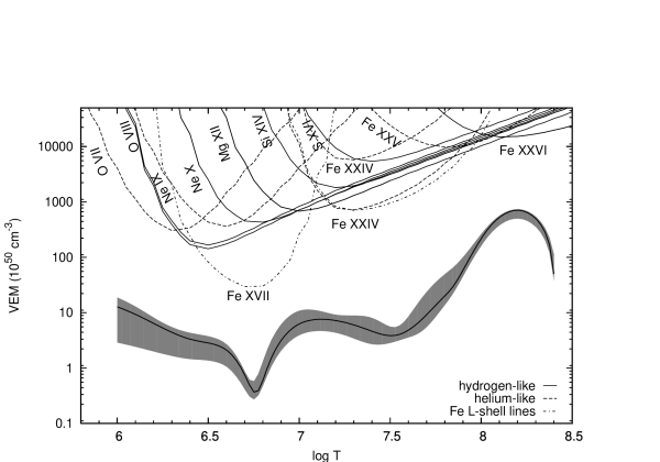
Figure 3: VEM as a function of temperature. The dashed lines, solid lines and dash-dot lines corresponds to VEM of helium-like, hydrogen-like and Fe-L shell lines respectively. The thick solid line is the DEM derived using MCMC(M) reconstruction technique on a set of lines of hydrogen-like, helium-like of different atoms and highly ionized Fe line fluxes assuming solar photospheric abundances. The shaded areas are the 95% confidence limits corresponding to each temperature bin.

Using Equation 1, we can calculate the maximum emission measure as a function of temperature for each emission line. The combination of emission measure of individual lines can be used to constrain the emission distribution of the source. The VEM estimated using Equation 1 for different lines are plotted in Figure 3. The emissivities of the lines are taken from APED (Smith et al., 2001). The curves are the loci corresponding to the VEM required to produce the observed flux from an isothermal plasma as a function of plasma temperature. At a given temperature, a point on one of these curves represents a maximum EM that the plasma can have at that temperature. The solid lines in the figure represent hydrogen-like lines of O, Ne, Mg, Si, S and Fe, dashed lines correspond to resonance lines of O VII, Ne IX and Fe XXV, whereas the dash-dot-dash lines represent the VEM of Fe L-shell lines.

The VEM defined in Eqn.1 in the logarithmic differential form is called as Differential Emission Measure (DEM). The DEM gives a correlation between the amount of emitting power and the amount of emitting material in the plasma as a function of temperature. The DEM was estimated by performing a Markov Chain Monte-Carlo analysis using a Metropolis algorithm (MCMC[M]) (kashyap, 1998) implemented in PINTofALE (kashyap, 2000) on the set of sixteen brightest lines in the AM Her spectrum. The MCMC(M) method gives an estimate of emission measure distribution over a pre-selected temperature region with the DEM defined for each bin. Here, we used a temperature grid ranging from $\log T=6.0$ to $\log T=8.8$ with $\Delta\log T=0.2$. The lower and the upper limit of the temperature region are choosen to represent the hydrogen and helium-like lines of O and, hydrogen and helium-like lines of Fe respectively, present in the spectrum. The intermediate temperatures are constrained by the L-shell lines of Fe, and helium-like lines of Ne, Mg, S and Si. The reconstructed DEM is plotted in Figure 3 with 95% confidence limits shown as shaded region.

2.4 Phase dependent variation of spectral lines

To look for modulations in the continuum and emission lines with the binary period, the data were folded using the ephemeris for the magnetic phase and a period of $0.128927$ days as given by Tapia (1977), and Young et al. (1981). Two methods were adopted to obtain the phase resolved spectra. In the first method, the spectra were extracted for five non-overlapping regions of 0.2 phase interval. Except for the interval centered around the orbital phase minima, other intervals had enough number of counts to estimate the line energy and the photon flux in many of the bright emission lines. From these spectra it was observed that while some lines showed shifts in the line energy with phase, others did not. The second method is based on extracting the spectra into continuous overlapping regions (See Hoggenwerf et al., 2004). In this method, the spectra were accumulated for twenty phase intervals of width $\Delta\Phi\ =\ 0.25$, with phase intervals starting at $\Phi_{0}$ = 0.0, 0.05, 0.1 $\ldots$, where, $\Phi$ is the orbital phase. Spectra obtained from both the methods were analysed for their continuum and emission line properties. The continuum was modelled using a bremsstrahlung after masking the regions of emission lines identified using APED.

Different regions of spectra were examined for studying the line emission properties as a function of phase. Figure 4 shows spectra for four non-overlapping phase bins in the wavelength region 1.75 - 2.0 $\mathrm{\AA}$ which covers the Fe XXVI line, Fe XXV ($r,\ i,$ and $f$), and the fluorescent line of Fe I. The best fit line energies were compared with the reference line energies to determine the shifts of different emission lines observed. The Fe XXVI line consists of a doublet, Ly$\alpha_{1}$ and Ly$\alpha_{2}$ at 6.973 and 6.952 keV respectively. The two lines can not be resolved with Chandra HEG resolution of $\sim 35eV$ at 7 keV. The branching ratio 2:1 of the Ly$\alpha_{1}$ and Ly$\alpha_{2}$ yield a line centroid of 6.966 keV (Pike et al. 1996; Hellier & Mukai 2004). This value was used as a reference to determine any shift in the Fe XXVI line energy. The stabilizing transitions of doubly excited ions lead to dielectronic recombination satellite (DES) lines redward of Fe XXVI lines. The Fe XXVI lines are mainly affected by a feature at 6.92 keV whose intensity is $\sim 8\%$ of the Fe XXVI lines at $5\times 10^{7}\$K and falls below 5% at $8\times 10^{7}\$K (Dubau et al., 1981). Hence the contribution of DES lines to Fe XXVI in AM Her can be neglected due to high plasma temperature of $1.8\times 10^{8}$ K ($\sim$15.6${}^{+5.2}_{-3.1}$ keV; the maximum temperature from 4T APEC fit from Table 1). The intensities of DES lines depend both on temperature and intensity of adjacent ionization states, specially Fe XXIV and Fe XXIII. At temperatures above $3.5\times 10^{7}$ K, the contribution of DES is negligible (Oelgoetzty & Pradhan, 2001), and hence, we did not consider the effects of DES lines. To include the contribution of unresolved $i$ lines and $f$ line, we used three Gaussians representing the $r$, $i$ and $f$ lines. For the calculation of line shifts in Fe XXV, we used the rest frame energy of $r$ at 6.700 keV, $i$ at 6.675 keV and $f$ at 6.636 keV.

The strength of DES lines approximately scales as $Z^{4}$ and hence, their effects have been neglected in the analysis of S, Si and Mg. We used 2.623, 2.005 and 1.473 keV as reference line energies for S XVI, Si XIV and Mg XII respectively.

From the phase resolved spectra, we found that the line centers of individual lines for different phase bins deviate from the predicted wavelengths. The difference between the observed and expected emission line center is used to calculate the Doppler shift of the emission line from different phase bins.

The calculated Doppler shifts of emission lines of Fe XXVI and Fe XXV (r) as a function orbital phase are plotted in Figure 5. Doppler shifts obtained from non-overlapping phase bins are shown as filled circles. The shifts from overlapping phase bins are shown for a better visualization only. The figure clearly shows a non-zero shift in the two lines. The amplitude of Doppler shift of different lines also shows a variation with orbital phase. The modulation in the shift in line center with phase is most clearly seen in Fe XXVI line as compared to the Fe XXV line. In order to quantify the observed modulation of the Doppler shifts with phase in the above mentioned lines a sinusoid+constant model was fitted to the data using $\chi^{2}$ minimization. To calculate the un-modulated velocity shift, we fit a sinusoid with non-zero mean to the observed modulation of all lines using non-linear least square fitting. We have also checked for the presence of any Doppler shifts in fluorescent Fe, S XVI and Mg XII lines. The mean Doppler velocity determined from the average spectrum of different lines are summarized in the second column of Table 3. The third and the fourth columns of Table 3 list a constant velocity shift and the amplitude of the sinusoid, respectively. The sinusoid best fit for different lines are superposed over the doppler shifts as dashed lines in Figure 5. For Fe XXVI we get a semi-amplitude of 790 $\pm$ 40 km s^-1 with a mean of 220 $\pm$26 km s^-1. Just to compare, we fit a constant model to the velocity shifts and list them in column five of Table 3. A constant fit to the Fe XXVI data gives a velocity shift 565$\pm$195 km s^-1, but the fit is considerably worse with a $\chi^{2}_{\nu}=3.29$ as compared to a $\chi^{2}_{\nu}=0.02$ for the sinusoid fit. The shifts in the Fe XXV (r), S XVI and Mg XII are however well fit with a constant velocity shift of 770 $\pm$ 75 km s^-1 ($\chi^{2}_{\nu}=0.06$), 500$\pm$160 km s^-1 ($\chi^{2}_{\nu}=0.79$), and 280$\pm$195 km s^-1 ($\chi^{2}_{\nu}=0.15$) respectively. The $\chi^{2}_{\nu}$ values for the constant fits and sinusoid fits are similar. The fluorescent Fe line shows no detectable shift, with $2\sigma$ upper limit of 400 km s^-1. The Si XIV line is too weak to determine the parameters accurately, therefore, no constraints are put on the shift of this line.

Although no modulation is apparent in the velocity shifts of the Fe XXV (r), S XVI, and Mg XII, the error bars on the shifts of their lines can not rule out the possibility of modulation being present at some level. To estimate the level of modulation, we have force fitted a constant plus a sinusoid component similar to the one used for Fe XXVI. The semi-amplitude of the sinusoid and the constant value for the velocity shifts of Fe XXV, S XVI and Mg XII are also listed in Table 3. The amplitude of modulation in these lines are of the order of the error bars.

3 Discussion

3.1 Average X-ray spectrum

Ratios of the line fluxes of helium-like lines provide good diagnostics of density and temperature of the line forming regions (Gabriel & Jordan, 1969; Porquet & Dubau, 2000). The transition from the excited ${}^{1}\mathrm{P}_{1},^{3}\mathrm{P}_{1}\,\mathrm{and}^{3}\mathrm{S}_{1}$ levels to the ground level ${}^{1}\mathrm{P}_{1}$ forms the three strongest lines of helium triplets: the resonance line (r), the intercombination line (i) and the forbidden line (f) respectively. The analytical relations between the electron density $R(n_{e})$ and temperature $G(T_{e})$ are, $R(n_{e})={f}/{i}$ and $G(T_{e})={(f+i)}/{r}$ (Gabriel & Jordan, 1969; bluementhal et al., 1972).

The He-like triplets of oxygen and neon are used as the diagnostics of low temperature regions. As we could not resolve the He-like lines of Fe, we do not use Fe XXV as a plasma diagnostic. We can only put an upper limit on the fluxes of ‘f’ lines of Ne IX and O VII and hence, we could only estimate the upper limits of the two ratios. The helium-like lines of Si, S and Mg are too weak in the spectrum and hence do not allow us to put any constraints on their G and R ratios. Using the values listed in Table 2, we get $R<0.48$ and $G<0.76$ for oxygen triplet and $R<0.5$ and $G<0.8$ for neon triplet, as 3$\sigma$ upper limits.

Comparing the measured $G(T_{e})$ values of O VII and Ne IX with the theoretical relation between $G(T_{e})$ and electronic temperatures (Porquet & Dubau, 2000) suggests a temperature greater than $\sim 2MK$. This temperature agrees with the lowest temperature of 0.13 keV (1.5 MK) of the four APEC components. Similarly comparing the measured values of $R(n_{e})$ with theoretically predicted values for a collisional dominated hybrid plasma implies a density greater than $2\times 10^{12}\ cm^{-3}$. Since the temperature and density of the O and Ne helium-like line emitting regions are very close, we assume that the emission of the two triplets takes place very close to each other. However, it should be noted that the presence of UV radiation fields can also mimic high densities as the transition from $f$ to $i$ can also be triggered by UV photons. Strong UV radiation is known to be present in AM Her (wesemael et al., 1980; Szkody et al., 1982).

The measured ratio of H- to He-like line intensities can be used to constrain the ionization temperature of the emitting plasma. We have used Fe ions to constrain the maximum ionization temperature in the post-shock region. A value of I(Fe XXVI)/I(Fe XXV) = 1.22 ${}^{+0.27}_{-0.21}$ suggests an ionization temperature of 12.4${}^{+1.1}_{-1.4}$ keV (Mewe et al, 1985). This matches well with the maximum electron temperature 15.6${}^{+5.2}_{-3.1}$ keV of AM Her obtained from 4-T APEC global fit. The agreement with the continuum temperature and ionization temperature is consistent with the results obtained using moderate energy resolution ASCA data (Ishida et al., 1997).

Volume emission measure analysis using individual lines shows that the plasma has a range of temperature from 1.5–100 MK. The absence of the N VI He-like triplet indicates an VEM distribution dominated by high temperatures. We obtain the lowest VEM from Fe XVII with 2.96$\times 10^{50}$ cm^-3 at $\log T=$ 6.8 ($\sim$6 MK), whereas the peak VEM of 9.73$\times 10^{53}$ cm^-3 from Fe XXVI is at $\log T=$ 8.2 ($\sim$63 MK). We also estimated the differential emission measure using the fluxes of sixteen strong lines. We obtain a well constrained DEM(T) between $\log T=6.0$ and $\log T=8.2$. The minimum of the DEM is around $\log T=6.6-6.8$ and there is an indication of a DEM maximum around $\log T=8.2$, but, the lack of sufficient number of lines in this region makes it ambiguous. Though the trial DEM ranges from $\log T=6.0$ to $\log T=8.8$, the lack of spectral information beyond $\log T=8.2$ makes it un-realistic. The 4-T APEC model provides only an approximate discrete representation of the continuous VEM distribution. The temperature distribution thus obtained is consistent with that determined using individual lines. The temperature with the lowest VEM/DEM determined by the former method agrees with the lowest VEM of 4-T model.

3.2 Phase resolved spectroscopy

According to the standard models of accretion in polars, supersonic matter in an accretion column forms a shock near the surface of the white dwarf heating up the post shock region to very high temperatures ($10^{8}$ K) thus emitting hard X-rays. As the post shock matter falls toward the white dwarf surface, it cools down while getting slowed down. A phase dependent change in the spectral shape of the continuum is consistent with a non-uniform temperature distribution expected in the accretion column of polars. The central energies of emission lines of different elements, particularly hydrogen-like ions of Mg, S and Fe appear to be shifted from their theoretically expected values, implying possible bulk motion in the post-shock region of AM Her. The velocity shift increases as the atomic number increases from Mg to Fe. The observed gradient in the velocities of different ionization states of different elements can be interpreted as a signature of cooling and the slowing down of the matter.

The physical conditions in the accretion column can be described by velocity (v), temperature (T), density ($n_{e}$), height and size of the accretion column (h, r). At the shock region, the values of these parameters depend only on the mass, radius and the accretion rate of the white dwarf (Aizu, 1973). The velocity shift observed in emission lines of different ionization states of different elements seen in the Chandra HEG spectra of AM Her gives us a unique tool for the determination of the structure of the accretion column of AM Her, using the relationships among the above listed parameters as given by Aizu (1973).

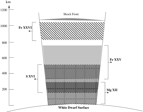
Figure 6: Schematic representation of positions (in km) of different line emitting regions in the accretion column of AM Her. The emitting regions are labelled. The width (in km) of individual emitting region corresponds to the errors shown in Table 3.

The accretion column parameters in the shock region, calculated using different mass estimates of AM Her ranging from 0.39–0.91 M_☉ reported in the literature, and an accretion rate of $\dot{m}$ = 0.4 g cm^-2 s^-1 (G$\ddot{a}$nsicke et al., 1995) are listed in Table 4. The radius of the white dwarf for each mass value was calculated using the mass-radius relation for white dwarfs (Nauenberg, 1972), and found to be in the range of 0.016–0.009 $R_{\sun}$. Using these values we estimated the values of parameters like shock velocity, $v_{sh}$, shock temperature, kT_sh and shock height, $h$, as listed in Table 4 (See Appendix A, Terada et al., 2001, for the relations of shock parameters with white dwarf mass, radius and accretion rate). We assumed the solar abundances for the elements and mean molecular weight of the in-falling gas, $\mu$ = 0.615, which corresponds to a mixture of hydrogen and helium in the ratio of 0.7 and 0.3 respectively. The calculated $v_{sh}$ for M${}_{wd}\ <$ 0.6 M_☉ is much less than the observed velocity shift of the Fe XXVI line. Thus, assuming the observed velocity of Fe XXVI as equal to $v_{sh}$, we obtain the mass of the white dwarf to be $\sim 0.6$ M_☉. This also puts some constraints on the geometry of the accretion column of AM Her by providing corresponding values of height and radius of the shock region. For a 0.6 $M_{\sun}$ white dwarf, we estimated the heights at which different emission lines are emitted in the accretion column and list them in the sixth column of Table 3. Figure 6 shows the schematic of the distribution of different line emitting regions in the accretion column from the white dwarf surface. Different shades/patterns in the figure correspond to different emission lines labelled in the figure and the width of each region corresponds to 90% confidence levels of the height of the emitting region for the particular ion.

A rough estimate about the upper limit on the white dwarf mass can be obtained using the fact that the heights at which different emission lines are emitted in the accretion column depend on the mass of white dwarf. Wu, Cropper & Ramsay (2001) have investigated the ionization structure of the post shock region of MCVs and predicted line emissivity profiles for Fe XXVI and Fe XXV lines for white dwarf masses of 1.0 M_☉ and 0.5 M_☉ assuming different magnetic field strengths ($\epsilon_{0}=0,1,10,100$). They show that highly ionized Fe lines are emitted close to the shock front for a low mass white dwarf with high magnetic fields, whereas they are formed well below the shock front for high mass white dwarfs. Though the emissivity structure depends on the white dwarf mass, the ratio of these heights will be independent of the mass of the white dwarf. Based on the observed velocities for Fe XXVI and Fe XXV line emitting regions, we calculate the ratio of the heights of these two lines and compare this with that obtained from line emissivity profiles (Figures 6 and 7 of Wu, Cropper & Ramsay, 2001). Here we assume that the height of the maximum emissivity region of a line coincides with the height determined from its bulk velocity. From Wu, Cropper & Ramsay (2001), the ratios are found to be $\sim 3$ and $\sim 5$ for white dwarf of mass 1.0 M_☉ and 0.5 M_☉ respectively. The ratio of the heights of these two lines in AM Her is $\sim 2$ indicating a mass closer to 1 M_☉.

Using the mean emissivity over the region of maximum emissivity of the four emission lines Fe XXVI, Fe XXV(r), S XVI and Mg XII taken from APED and adopting a distance of 91 pc for AM Her, we obtain an average VEM of 2.54$\times 10^{54}$ cm^-3. Using this VEM and the values of kT_sh and $h$ listed in Table 4, we determine the electron density, n${}^{sh}_{e}$ at the shock and the radius of the shock region, r_sh, and list them in Table 4.

In polars, the accreting matter is assumed to be streaming along the magnetic poles. The bulk motion velocity ($v$) of this matter will be seen from different angles along the line of sight due to the rotation of the white dwarf. The apparent velocity of accreting matter at any orbital phase $\Phi$ is given by $v_{\Phi}=v\cos\theta$, where, $\theta$ is the angle between the magnetic axis and line of sight, and is related to the inclination angle $i$, magnetic obliquity $\beta$ and $\Phi$ as

$$\cos\theta\ =\ \cos i\ \cos\beta\ -\ \sin i\ \sin\beta\ \cos(\Phi+\pi/2)$$ (2)

Assuming $i=35^{\circ}\pm 5^{\circ}$ and $\beta$ = $58^{\circ}\pm 5^{\circ}$ (Brainerd & Lamb, 1985), the observed modulation in the velocity of Fe XXVI line can be well explained by Equation 2 with the emitting region moving at a velocity of $\sim\!1100$ km s^-1 accreting on to a single pole. This velocity is close to the shock velocity of an accreting white dwarf of mass in the range of 0.6–0.7 $M_{\sun}$. Thus, we interpret the observed variation in the amplitude of line shifts with phase as due to the aspect effect according to Equation 2. Similar phase dependent line velocity variation of few hundred km s^-1 are reported in several FUV lines too (G$\ddot{a}$nsicke et al., 1998; Mauche & Raymond, 1998; Hutchings et al., 2002). Also, observations with Low Energy Transmission Grating onboard Chandra X-ray observatory showed that the emission line components are somewhat broader than the instrumental width, and the authors attribute this to the continuously changing angle between the accretion column and the observer (Burwitz et al, 2001).

The apparent lack of any velocity shift in the fluorescent line is in accordance with the standard emission models where this line is believed to be due to reflection of the hard X-rays from the surface of the white dwarf. The equivalent width of Fe fluorescent line ($\sim 150$ eV) combined with an N_H smaller than 10⁺²¹ cm^-2 also supports this idea (Ezuka & Ishida, 1999).

In the above discussion we assume that the observed velocity shifts are real and not an artefact. This can be judged from Figure 4 that clearly shows the varying line center of Fe XXVI and Fe XXV. Also the shifts in the line center values obtained from the overlapping phase bins (Figure 5) clearly show a sinusoidal trend modulated with the orbital period. The one artefact that might get introduced into our analysis is wrong identification of a particular line as the wavelength region around 1.6-2.0 $\AA$ is filled with many DES and other lines. Though the resolution of Chandra HEG data does not allow us to fully resolve individual He-like lines of Fe, and wrong identification of a line is plausible, the effect of this is only to change the final velocity value but not the modulation.

4 Conclusions

We have presented here an analysis of high resolution Chandra observations of a prototype polar AM Her. The analysis of the average X-ray spectrum shows that it is well fitted by a multi-temperature, partially absorbed plasma emission APEC models. A mass of 1.15$\pm$0.05 M_☉ is derived based on the best fit of multi-temperature plasma model to the average X-ray spectrum of AM Her. The multi-temperature nature of the plasma is further confirmed by analysis of individual emission lines. The plasma diagnostics based on line-ratios of helium-triplets and Fe-L shell ions suggests a dense ($>2\times 10^{12}$ cm^-3) plasma. The helium-like triplets of O and Ne give a temperature of $>$2 MK, whereas the ratio of hydrogen-like line to helium-like line of Fe suggests a temperature of 12 keV. We have constructed the DEM distribution of a AM Her, which is the first time that such an exercise has been carried out for a polar. The constructed DEM distribution using individual line fluxes shows that the DEM is continuous with a possible minimum near $\log T=6.8$.

From the phase resolved spectroscopy, we have found a possible evidence for bulk motion of the ionized material in the accretion column of AM Her. The velocity of Fe XXVI line is modulated as a function of the orbital phase consistent with a single pole accretion. The Fe XXVI ions from the hottest plasma show a maximum velocity shift of $\sim$1100 km s^-1, that is close to the shock velocity expected for a $\sim$0.6 M_☉ white dwarf. The velocity shifts are observed to be much smaller for Fe XXV(R), and the hydrogen-like lines of S XVI and Mg XII. The variation in the velocity shifts of different ions is used to calculate the height of the accretion column from the white dwarf surface from where the line emission originates. An mass of $\sim$1.0 M_☉ for the mass of the white dwarf is indicated by using the heights of Fe XXVI and Fe XXV line emitting regions estimated by the observed velocities of these lines. The multi-temperature mass estimate hence, gives an upper limit for the mass of the white dwarf owing to the bias introduced by using single temperature flow in the accretion column. The density and temperature structure in the accretion column are also derived. No velocity shift is seen in the fluorescent Fe line, consistent with its origin due to reflection from the white dwarf surface. Higher resolution observations are required to detect the radial velocity modulation in this line.

Table 1: Spectral parameters for the best fit 4-T APEC model to the average spectrum of AM Her. The VEM is calculated for a distance of 91 pc.

APEC	kT	log(T)	$\chi^{2}$	Dof	VEM
	(keV)	(K)			($\times 10^{53}$cm${}^{-3})$
1	0.13${}^{+0.03}_{-0.08}$	6.17${}^{+0.10}_{-0.39}$	1747	2767	1.28${}^{+2.55}_{-0.57}$
2	0.65${}^{+0.08}_{-0.08}$	6.88${}^{+0.05}_{-0.06}$	1716	2765	0.25${}^{+0.38}_{-0.09}$
3	2.7${}^{+0.6}_{-0.4}$	7.50${}^{+0.08}_{-0.08}$	1654	2763	3.36${}^{+5.19}_{-1.26}$
4	15.6${}^{+5.2}_{-3.1}$	8.26${}^{+0.12}_{-0.10}$	1624	2761	25.4${}^{+25.8}_{-3.1}$

Table 2: Measured fluxes, equivalent widths and Ionic column densities of the emission lines identified in the HETG spectrum of AM Her.

Ion	Wavelength	Energy	Flux	Equivalent Width
	$\mathrm{(\AA)}$	$(keV)$	$(10^{-5}\ photon\ cm^{-2}\ s^{-1})$	$(eV)$
Fe XXVI	$~{}1.781^{+0.001}_{-0.002}$	$6.956^{-0.001}_{+0.009}$	$9.3^{+1.8}_{-1.3}$	173
Fe XXV (r)	$~{}1.853^{+0.001}_{-0.001}$	$6.691^{+0.002}_{-0.005}$	$7.6^{+0.9}_{-0.8}$	104
Fe I $K_{\alpha}$	$~{}1.937^{+0.002}_{-0.001}$	$6.402^{+0.006}_{-0.002}$	$9.3^{+1.6}_{-1.0}$	151
S XVI	$~{}4.735^{+0.002}_{-0.001}$	$2.619^{+0.001}_{-0.001}$	$2.6^{+0.6}_{-0.5}$	17.9
S XV	$~{}5.038^{+0.001}_{-0.016}$	$2.461^{+0.001}_{-0.008}$	$0.8^{+0.3}_{-0.4}$	5.2
Si XIV	$~{}6.184^{+0.001}_{-0.001}$	$2.005^{+0.001}_{-0.001}$	$2.5^{+0.3}_{-0.3}$	12.2
Mg XII	$~{}8.424^{+0.001}_{-0.001}$	$1.472^{+0.001}_{-0.001}$	$1.2^{+0.2}_{-0.2}$	3.9
Fe XXIV	$10.625^{+0.004}_{-0.001}$	$1.167^{+0.001}_{-0.001}$	$1.2^{+0.2}_{-0.2}$	3.9
Fe XXIV	$11.181^{+0.084}_{-0.002}$	$1.109^{+0.008}_{-0.001}$	$1.3^{+0.3}_{-0.4}$	2.8
Fe XXIV	$11.432^{+0.033}_{-0.144}$	$1.085^{+0.003}_{-0.014}$	$0.8^{+0.3}_{-0.4}$	1.7
Fe XXII2	11.78	1.055	$<0.3$
Fe XXII2	11.92	1.040	$<0.6$
Ne X 1	$12.139^{+0.055}_{-0.002}$	$1.022^{+0.005}_{-0.001}$	$2.8^{+0.5}_{-0.5}$	5.5
Ne IX (r)	$13.452^{+0.136}_{-0.001}$	$0.922^{+0.009}_{-0.001}$	$1.5^{+0.7}_{-0.4}$	2.5
Ne IX (i)	$13.544^{+0.225}_{-0.031}$	$0.916^{+0.015}_{-0.002}$	$0.8^{+0.7}_{-0.3}$	1.3
Ne IX (f)2	$13.544^{+0.225}_{-0.031}$	$0.905^{+0.000}_{-0.000}$	$<0.6$
Fe XVII	$15.012^{+0.022}_{-0.091}$	$0.826^{+0.001}_{-0.005}$	$1.0^{+0.7}_{-0.6}$	1.5
Fe XIII	$16.021^{+0.851}_{-0.851}$	$0.774^{+0.041}_{-0.041}$	$1.2^{+0.9}_{-0.6}$	2.2
Fe XVII	$17.056^{+0.065}_{-0.065}$	$0.727^{+0.004}_{-0.004}$	$1.8^{+1.1}_{-0.9}$	5.6
Fe XVII	17.100	0.725	$0.6^{+0.9}_{-0.6}$
O VIII	$18.966^{+0.193}_{-0.193}$	$0.654^{+0.001}_{-0.001}$	$9.8^{+2.5}_{-2.5}$	19.8
O VII (r)	$21.603^{+0.130}_{-0.548}$	$0.574^{+0.003}_{-0.005}$	$14.7^{+4.6}_{-4.1}$	18.2
O VII (i)	$21.812^{+0.013}_{-0.001}$	$0.569^{+0.001}_{-0.001}$	$7.5^{+4.2}_{-3.0}$	9.6
O VII (f)2	$22.064$	$0.562$	$<$3.6

Table 3: Measured line velocity shifts of emission lines and corresponding heights of emitting regions of AM Her

Line Id	V${}^{(1)}_{avg}$	V${}^{(2)}_{\Phi,\ const}$	V${}^{(2)}_{\Phi,\ mod}$	$V^{(3)}_{l}$	Height
	(km s-1)	(km s-1)	(km s-1)	(km s-1)	(km)
Fe XXVI	430$\pm 130$	220$\pm$ 26	790$\pm$40	565$\pm$195	932$\pm$110
Fe XXV(r)	850$\pm 90$	660$\pm$ 70	145$\pm$110	770$\pm$75	529$\pm$213
S XVI	510$\pm 80$	545$\pm$140	110$\pm$120	500$\pm$160	315$\pm$220
Mg XII	190${}^{+140}_{-270}$	240$\pm$160	180$\pm$140	280$\pm$195	105$\pm$130

Table 4: Parameters of shock in accretion column of AM Her

Mwd	Rwd	$v_{sh}$	kTsh	$h$	n${}^{sh}_{e}$	rsh
(M☉)	(R☉)	(km s-1)	(keV)	(km)	(1015 cm-3)	(km)
0.39	0.016	765	11.3	394	3.4	2556
0.50	0.014	922	16.4	691	2.3	2806
0.60	0.013	1066	21.9	1067	1.7	3017
0.75	0.011	1290	32.1	1889	1.2	3318
0.91	0.009	1555	46.7	3312	0.8	3643

Figure 1: Chandra HETG spectrum of AM Her for the summed +1 and -1 orders. Only HEG spectrum is plotted for clarity. Data plotted are smoothed by a Gaussian convolution of width 0.0025 $\mathrm{\AA}$ HEG. The data are shown as histograms and the dashed line represents line-by-line fit to the data. Gaussians are used to model individual emission lines from various ionized elements and the continuum is modelled by an unabsorbed bremsstrahlung model.

Figure 2: Same as Figure 1, showing only MEG data. Here data are smoothed by a Gaussian convolution of width 0.005 $\mathrm{\AA}$.

Figure 4: Gaussian fits (dashed lines) to the observed (histogram) Fe XXVI, Fe XXV (r,i & f) and fluorescent Fe lines. The orbital phase is shown in the inset. The width of each phase bin, $\Delta\Phi$ = 0.2.

Figure 5: Plot of the velocity shifts as a function of orbital phase for the emission lines Fe XXVI and Fe XXV as described in the text. The filled circles correspond to the velocity shifts observed in the non-overlapping phase intervals with $\Delta\Phi$ = 0.2.

References

- Aizu (1973) Aizu, K., 1973, Prog. Theor, Phys., 49, 1184
- Arnaud (1996) Arnaud, K., in ASP Conf. Ser. 101, Astronomical Data Software & Systems V, 1996, ed. G.H. Jacoby & J. Barnes (San Fransisco: ASP), p17
- Brainerd & Lamb (1985) Brainerd, J. J., & Lamb, D. Q., 1985, in Cataclysmic Variables and Low-Mass X-ray Binaries, ed. D. Q. Lamb and J. Patterson (Dordrecht: D. Reidel), p247
- bluementhal et al. (1972) Bluementhal, G.R., Drake, G.W.F., Tucker, W.H., 1972, ApJ, 172, 205
- Burwitz et al (2001) Burwitz, V., Reinsch, K., Barwig, H., 2001, Astronomische Gesellschaft Abstract Series, 18, 192
- Canizares et al. (2005) Canizares, C. R., Davis, J. E., Dewey, D., et al., 2005, PASP, 117, 1144
- Cropper, Ramsay & Wu (1998) Cropper M., Ramsay G., & Wu K., 1998, MNRAS, 293, 222
- Cropper et al. (1999) Cropper, M., Wu, K., Ramsay, G., & Kocabiyik, A., 1999, MNRAS, 306, 684
- Dubau et al. (1981) Dubau, J., Gabriel, A.H., Loulergue, M., Steenman-Clark, L., & Volonté, S., 1981, MNRAS, 195, 705
- Ezuka & Ishida (1999) Ezuka, H., & Ishida, M., 1999, ApJs, 120, 277
- Gabriel & Jordan (1969) Gabriel, A.H., Jordan, C., 1969, MNRAS, 145, 241
- Gnsicke et al. (1995) Gnsicke, B. T., Beuermann, K., & D, de Martino, 1995, A&A, 303, 127
- Gnsicke et al. (1998) Gnsicke, B. T., Hoard, D. W., Beuermann, K., Gansicke, B. T., Hoard, D. W., Beuermann, K., Sion, E. M., & Szkody, P., 1998, A&A, 338, 933
- Garmire et al. (2003) Garmire, Gordon P., Bautz, Mark W., Ford, Peter G., Nousek, John A., & Ricker, George R. Jr., 2003, SPIE, 4851, 28
- Griffiths & Jordan (1998) Griffiths. N.W., & Jordan, C., 1998, ApJ, 497, 883
- Hellier & Mukai (2004) Hellier, C., & Mukai, K., 2004, MNRAS, 352, 1037
- Hoggenwerf et al. (2004) Hoggenwerf, R., Brickhouse, N. S., & Mauche, C. W., 2004, ApJ, 610, 411
- Hutchings et al. (2002) Hutchings, J. B., Fullerton, A. W., Cowley, A. P., & Schimidtke, P. C., 2002, AJ, 123, 2841
- Huenemoerder (2003) Huenemoerder, David P., Canizares, Claude R., Drake, Jeremy J., & Sanz-Forcada, Jorge., 2003, ApJ, 595, 1131
- Ishida et al. (1997) Ishida, M., Matsuzaki, Keiichi., Fujimoto, R., Mukai, K., & Osborne, J. P., 1997, MNRAS, 287, 651
- kashyap (1998) Kashyap, V. & Drake, J.J., 1998, ApJ, 503, 450
- kashyap (2000) Kashyap, V. & Drake, J.J., 2000, BASI, 28, 475
- Mauche & Raymond (1998) Mauche, C. W., & Raymond, J. C., 1998, ApJ, 505, 869
- Mattei et al. (1980) Mattei, J. A., Mayer, E. H., & Baldwin, M. E., 1980, S&T, 60, 180
- Mewe et al (1985) Mewe, R., Gronenschild, E.H.B.M., van den Oord, G.H.J., 1985, A&AS, 62, 197
- Mouchet (1993) Mouchet M., 1993, in White Dwarfs: Advances in Observation & Theory, ed. Barstow, M., p. 411 (Dordrecht: Kluwer)
- Mukai & Charles (1987) Mukai K., & Charles P. A., 1987, MNRAS, 226, 209
- Nauenberg (1972) Nauenberg, M., 1972, ApJ, 175, 417
- Oelgoetzty & Pradhan (2001) Oelgoetzty, J., & Pradhan, A.K., 2001, MNRAS, 327, L42
- Pike et al. (1996) Pike, C.D., Philips, J.H., & Lang, J., 1996, ApJ, 464, 487
- Porquet & Dubau (2000) Porquet, D., and Dubau, J., 2000, A&AS, 143, 495
- Saxton et al. (2005) Saxton, C.J., Wu, K., Cropper, M., Ramsay, G., 2005, MNRAS, 360, 1091
- Smith et al. (2001) Smith, R. K., Brickhouse, N. S., Liedahl, D. A., & Raymond, J. C., 2001 Spectroscopic Challenges of Photoionized Plasmas, ASP Conf. Series 247, p159. ed. Gary Ferland and Daniel Wolf Savin
- Szkody et al. (1982) Szkody, P., Raymond, J.C., Capps, R.W., 1982, ApJ, 257, 686
- Tapia (1977) Tapia, S., 1977, ApJ, 212, 125
- Terada et al. (2001) Terada, Y., Ishida, M., Makishima, K., Imanari, T., Fujimoto, R., Matsuzaki, K., & Kaneda, H., 2001, MNRAS, 328, 112
- wesemael et al. (1980) Wesemael, F., Auer, L.H., Van Horn, H.M., Savedoff, M.P., 1980, ApJ Suppl., 43, 159
- Wu, Changmugam & Shaviv (1995) Wu K., Changmugam G., & Shaviv G., 1995, ApJ, 455, 260
- Wu, Cropper & Ramsay (2001) Wu, K., Cropper, M., Ramsay, G., 2001, MNRAS, 327, 208
- Young et al. (1981) Young, P., Donald P. S., & Stephen A. S., 1981, ApJ, 245, 1043