Weak Gravitational Lensing with COSMOS: Galaxy Selection and Shape Measurements

Abstract

With a primary goal of conducting precision weak lensing measurements from space, the COSMOS^⋆ survey has imaged the largest contiguous area observed by the Hubble Space Telescope (HST) to date using the Advanced Camera for Surveys (ACS). This is the first paper in a series where we describe our strategy for addressing the various technical challenges in the production of weak lensing measurements from the COSMOS data. We first construct a source catalog from 575 ACS/WFC tiles (1.64 degrees²) sub-sampled at a pixel scale of 0.03″. Defects and diffraction spikes are carefully removed, leaving a total of $1.2\times 10^{6}$ objects to a limiting magnitude of $F814W=26.5$. This catalog is made publicly available. Multi-wavelength follow-up observations of the COSMOS field provide photometric redshifts for 73% of the source galaxies in the lensing catalog. We analyze and discuss the COSMOS redshift distribution and show broad agreement with other surveys to $z\sim 1$. Our next step is to measure the shapes of galaxies and to correct them for the distortion induced by the time varying ACS Point Spread Function and for Charge Transfer Efficiency effects. Simulated images are used to derive the shear susceptibility factors that are necessary in order to transform shape measurements into unbiased shear estimators. For every galaxy we derive a shape measurement error and utilize this quantity to extract the intrinsic shape noise of the galaxy sample. Interestingly, our results indicate that the intrinsic shape noise varies little with either size, magnitude or redshift. Representing a number density of $66$ galaxies per arcminute², the final COSMOS weak lensing catalog contains $3.9\times 10^{5}$ galaxies with accurate shape measurements. The properties of the COSMOS weak lensing catalog described throughout this paper will provide key input numbers for the preparation and design of next-generation wide field space missions.

1 Introduction

As we look towards distant galaxies, fluctuations in the intervening mass distribution cause a slight, coherent distortion of their intrinsic shapes. This effect, known as weak gravitational lensing, has been used for more than a decade to probe the cosmography and the growth of structure (for a review, see Bartelmann & Schneider, 2001). Although technically challenging because the weak lensing signal is minuscule and buried in a considerable amount of noise, this field has shown substantial progress due to the advent of high resolution space based imaging, the proliferation of wide-field multi-color surveys, and a determined effort to improve image analysis methods and minimize systematic errors through the Shear TEsting Program (STEP; Heymans et al., 2006; Massey et al., 2006).

Historically first observed only around cluster cores (Tyson et al., 1990), weak lensing has emerged as a versatile and effective technique to probe the mass distribution of clusters (e.g., Kneib et al., 2003), to measure the clustering of dark matter around galaxies ensembles (e.g., Natarajan et al., 1998; Hoekstra et al., 2004; Sheldon et al., 2004; Mandelbaum et al., 2005), and to put constraints on the matter density parameter $\Omega_{m}$ and the amplitude of the matter power spectrum $\sigma_{8}$ (e.g., Hoekstra et al., 2006; Semboloni et al., 2006; Schrabback et al., 2006; Hetterscheidt et al., 2006; Jarvis et al., 2006). Most applications currently only use the first order deformation induced by the mass distribution, but novel techniques are under development to take into account second order deformations (also called flexion; Goldberg & Bacon, 2005; Bacon et al., 2006; Okura et al., 2006; Goldberg & Leonard, 2006) and may prove to be more efficient probes of compact structures such as galaxies and groups of galaxies. Weak lensing measurements are particularly powerful when combined with the knowledge of the three dimensional galaxy distribution. Sophisticated lensing ’tomography’ techniques that utilize redshifts to analyze the 3D shear field are a sensitive probe of the growth of structure and the equation of state of dark energy (Jain & Taylor, 2003; Bernstein & Jain, 2004; Bacon et al., 2005). Applied in many different ways, weak lensing techniques unravel the mass distribution of structures and their evolution in the universe.

High quality measurements of weak shear depend on the accurate determination of the shapes and redshifts of distant, faint galaxies. The COSMOS program has imaged the largest contiguous area (1.64 degrees²) with the Hubble Space Telescope (HST) to date using the Advanced Camera for Surveys (ACS) Wide Field Channel (WFC). The Full Width Half Maximum (FWHM) of the Point Spread Function (PSF) of the ACS/WFC is $0.12\arcsec$ at the detector, yielding a much better resolution of small galaxies than ground-based surveys, which are typically limited by the seeing to a PSF of FWHM $\sim 1\arcsec$. Shape measurements also benefit from ACS/WFC imaging compared to ground-based observations because smaller corrections are required for the PSF and the shear measurements are less diluted by PSF smearing. The imaging quality and unprecedented area of the COSMOS ACS/WFC data combined with extensive follow-up observations at other wavelengths (Scoville et al., 2007; Koekemoer, 2007) to provide accurate photometric redshifts (Mobasher et al., 2007), make COSMOS a unique data set for weak lensing studies.

To exploit the weak lensing potential of the COSMOS ACS/WFC data, a carefully designed catalog of resolved galaxies with shape measurements must be extracted from the imaging data. The challenges and requirements of such a catalog are the following. First, the large survey size makes a robust automation of catalog generation essential. Second, the lensing sensitivity increases with the number density of resolved faint galaxies. Thus, it is important to detect all galaxies to faint magnitudes while taking care to minimize spurious detections that will add noise to weak lensing measurements. Third, the high spatial resolution of the ACS/WFC allows for an excellent separation of close pairs. Given accurate deblending and a high number density of galaxies, one can expect to measure shear statistically on sub-arcminute scales, where baryonic physics may begin to influence the dark matter distribution. As the COSMOS-ACS/WFC data set is likely to be the only large space-based lensing survey until the launch of next-generation wide field space missions such as snap or dune (Réfrégier et al., 2006), the knowledge acquired through the COSMOS data will be unique and of crucial importance for the preparation and design of these future missions.

This is the first paper of a series describing the galaxy selection, the galaxy shape measurement, the lensing analysis, and the cosmological interpretation of COSMOS data. Details regarding PSF corrections as well as tests for systematic effects are presented in the second paper of this series (Rhodes et al., 2007). A three dimensional cosmic shear analysis is presented in the third paper of this series (Massey et al., 2007). Finally, a fourth paper presents high resolution dark matter mass maps of the COSMOS field (Massey et al., 2007a).

In this paper, we describe our methods for constructing a galaxy catalog from the ACS/WFC data, to be used in subsequent weak lensing work with COSMOS. Our goal is to produce a catalog of galaxies with photometric redshifts and PSF-corrected shape measurements, free of contaminating stars, cosmic rays, diffraction spikes, and other artifacts. The paper is organized as follows. In $\S$2 we present the data. In $\S$3 we describe the pipeline that locates and measures the properties of all detected objects. In $\S$4, we assess the quality of the data and analyze the COSMOS redshift distribution. In $\S$5 and $\S$6 we present the PSF and CTE correction schemes, the shape and shear measurement methods, and our selection criteria for the final lensing catalog. In $\S$7 we extract the intrinsic shape noise of the galaxy sample as a function of redshift and discuss the implications for future weak lensing surveys. Where necessary, we assume a standard cosmological model with $\Omega_{\rm M}=0.3$, $\Omega_{\Lambda}=0.7$, $H_{0}=100h$ km s^-1 Mpc^-1 and $h=0.7$.

2 The COSMOS ACS Data

The COSMOS HST ACS field (Scoville et al., 2007; Koekemoer, 2007) is a contiguous 1.64 degrees², centered at 10:00:28.6, +02:12:21.0 (J2000). Between October 2003 and June 2005 (HST cycles 12 and 13), the region was completely tiled by 575 adjacent and slightly overlapping pointings of the ACS/WFC (see Figure 1). Images were taken through the wide F814W filter (“Broad I”). The camera has a $203\arcsec\times 203\arcsec$ field of view, covered by two 4096x2048 CCD chips with a native pixel scale of $0.05\arcsec$ (Ford et al., 2003). The median exposure depth across the field is 2028 seconds (one HST orbit). At each pointing, four 507 second exposures were taken, each dithered by 0.25$\arcsec$ in the $x$ direction and 3.08$\arcsec$ in the $y$ direction from the previous position. This strategy ensures that the 3$\arcsec$ gap between the two chips is covered by at least three exposures and facilitates the removal of cosmic rays. Pointings were taken with two approximately $180\arcdeg$ opposed orientation angles (PA_V3$=100\pm 10\arcdeg$ and $290\pm 10\arcdeg$). In this paper we use the “unrotated” images (as opposed to North up) to avoid rotating the original frame of the PSF. By keeping the images in the default unrotated detector frame, they can be stacked to map out the observed PSF patterns. For similar reasons, we perform detection in individual ACS/WFC tiles instead of on a larger mosaic (where the orientation of the PSF frame would be unknown). Figure 2 shows a COSMOS/ACS pointing with the bright detections ($F814W<23$) and the masking of stars, asteroid trails and image defects (see $\S$3.5).

To build our catalog, we use version 1.3 of the “unrotated” ACS/WFC data which has been specially reduced for lensing purposes (see Koekemoer, 2007, for technical details). Image registration, geometric distortion, sky subtraction, cosmic ray rejection and the final combination of the dithered images were performed by the MultiDrizzle algorithm (Koekemoer et al., 2002). As described in (Rhodes et al., 2007), the MultiDrizzle parameters have been chosen for precise galaxy shape measurement in the co-added images. In particular, a finer pixel scale of $0.03\arcsec/$pix was used for the final co-added images (7000x7000 pixels), even though this implies more strongly correlated pixel noise (see §3.8). Hereafter, when we refer to pixels, we will assume a pixel scale of $0.03\arcsec/$pix. Pixelization acts as a convolution followed by a re-sampling and, although current shear measurement methods can successfully correct for convolution, the formalism to properly treat re-sampling is still under development for the next generation of methods. Again following the recommendations of Rhodes et al. (2007), a Gaussian and isotropic multidrizzle convolution kernel was used, with scale=0.6 and pixfrac=0.8, small enough to avoid smearing the object unnecessarily while large enough to guarantee that the convolution dominates the re-sampling. This process is then properly corrected by existing shear measurement methods.

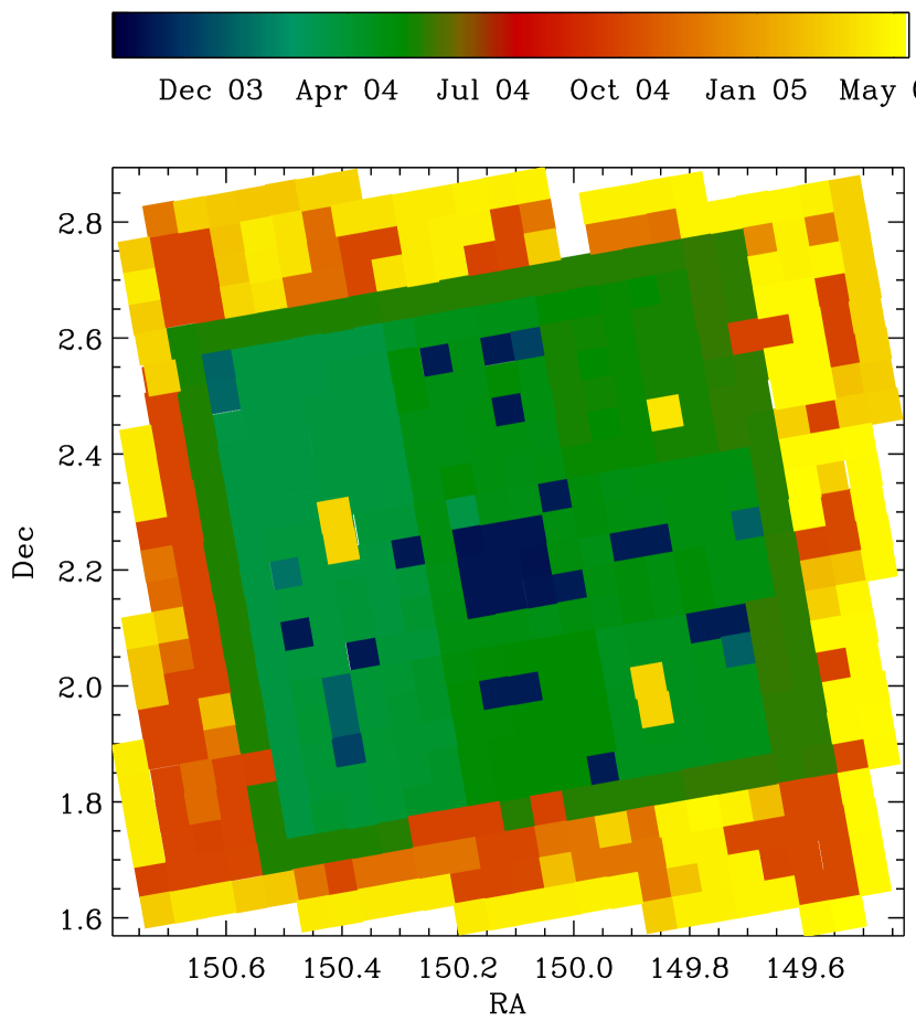
Figure 1: Date of observation for each of the survey pointings. The PSF of the ACS/WFC varies on timescales that are much shorter than the period over which COSMOS was observed.

The ACS/WFC CCDs also suffer from imperfect charge transfer efficiency (CTE) during read-out. As charges are transferred during the read-out process, a certain fraction are retained by charge traps (created by cosmic ray hits) in the pixels. This causes flux to be trailed behind objects as the traps gradually release their charge, spuriously elongating them in a coherent direction that mimics a lensing signal. Since this effect is produced by a fixed number of charge traps within the CCD substrate, it affects faint sources (with a larger fraction of their flux being trailed) more than bright ones. This is an insidious effect that mimics an increasing shear signal as a function of redshift, and prevents the traditional way of dealing with the calibration of faint galaxies in a lensing analysis by looking at bright stars. Ideally this effect would be corrected for on a pixel-by-pixel basis in the raw images unfortunately our current physical understanding of this effect is insufficient and a more indepth analysis in still underway. The CTE effect can be quantified sufficiently well however that, in a first step, we can adopt a post-processing correction scheme based on an object’s position, flux, and date of observation. Further details regarding this model can be found in Rhodes et al. (2007).

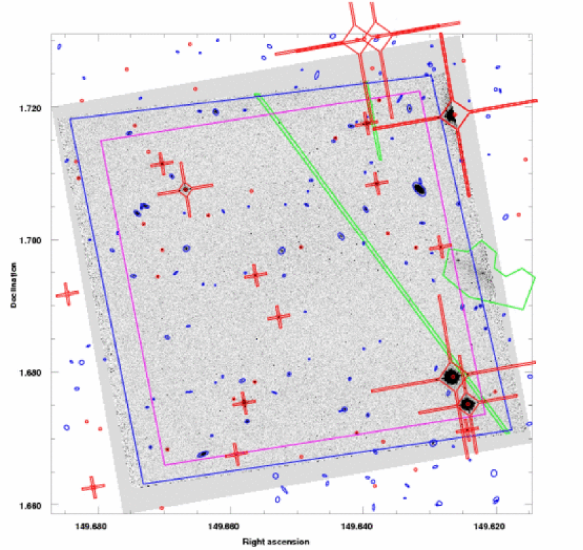
Figure 2: COSMOS pointing acs_I_095836+0141_unrot_sci_12.fits with bright detections, masking and edge definition indicated. Adjacent images have a sizable overlap (shown here by the smaller magenta box) which allows us to discard detections on the boundaries of each tile (defined by the larger blue box) without losing any objects in the final concatenated catalog. The automated masking of the diffraction spikes around bright stars ($F814<23$) is pictured here by the red polygons. The basic shape of the star masks is predefined and then scaled with the magnitude of the star. The green rectangles correspond to the manual masking of asteroid trails and various other image defects. Toward the right edge of this image, the dwarf galaxy L1-099 (Impey et al., 1996) is identified and flagged in a special category. Bright galaxies with $F814<23$ are depicted by blue ellipses and bright stars with $F814<23$ by red circles.

3 The COSMOS ACS Galaxy Catalog

In this section, we discuss the construction of the COSMOS ACS/WFC source catalog. This catalog is carefully cleaned of defects and artifacts and is made publicly available through the Infrared Science Archive (IRSA) database.

3.1 Detection Strategy

%̃ν which is independent of the shape of the ob ject. For an image of

We use Version 2.4.3 of the SExtractor photometry package (Bertin & Arnouts, 1996) to extract a source catalog of positions and various photometric parameters. In the construction of this catalog, our main concern is to pick out the small faint objects that contain most of the lensing signal. The detection strategy that we therefore adopt is to configure SExtractor with very low thresholds (even if this leads to more false detections in the catalog) and to control our sample selection via subsequent “lensing cuts” (see Sect 6). We hope to thus reduce unknown selection biases introduced by the SExtractor detection algorithm. When configured with low detection thresholds however, SExtractor also inevitably a) overdeblends low surface brightness spirals and patchy irregulars, b) deblends the outer features of bright galaxies, c) detects spurious objects in the scattered light around bright objects and d) underdeblends close pairs.

The correct detection of close pairs enables lensing measurements on very small scales. However, overdeblending and spurious detections adds noise to these measurements. In particular, false detections around bright objects can have quite high signal-to-noise ($S{\rm/}N$) values and are not trivial to remove with lensing cuts ( see $\S$6). The method presented here is a partial solution to b) c) and d). The overdeblending of low surface brightness and patchy galaxies remains a difficult problem, however, especially for high resolution imaging, and calls for an improvement of existing detection algorithms. With the advent of high resolution multi-wavelength surveys, a possible solution forward would be to incorporate color and morphological information into the detection process (e.g., Lupton et al., 2001).

While this overdeblending problem persists in our catalog, it affects less than $1\%$ of the objects. This problem is furthermore mitigated by the centroiding process during the shape measurement stage. Indeed, objects for which the centroid algorithm fails to converge, which will often be the case for overdeblended features, are discarded from the catalog. To remedy the remaining problems b) c) and d), we adopt and improve the method (known as the ‘Hot-Cold‘ method) employed in Rix et al. (2004). In this method, we run SExtractor twice, once with a configuration optimized for the detection of only the brightest objects (“cold” step) and then again with a configuration optimized for the faint objects (“hot” step). This double extraction helps improve the detection of close pairs. The two samples are then merged together to form the final catalog and masks are created around the bright detections minimizing the effects of c) and d).

For the “hot” and “cold” steps we vary four main parameters to optimize the detection: 1) detect_threshold, the minimum signal-to-noise per pixel above the background level, 2) min_area, the number of contiguous pixels exceeding this threshold, 3) back_size, the mesh size of the background map, 4) deblend_nthres and deblend_mincont, the parameters regulating deblending. In both cases, the data are filtered prior to detection by a 5 pixel (0.15″) Gaussian filtering kernel. Our choice of parameters for both steps is provided in Table 1.

Table 1: SExtractor configuration parameters

Parameter	Bright objects	Faint objects
DETECT_MINAREA	140	18
DETECT_ THRESH	2.2	1.0
DEBLEND_ NTHRESH	64	64
DEBLEND_MINCONT	0.04	0.065
CLEAN_PARAM	1.0	1.0
BACK_SIZE	400	100
BACK_FILTERSIZE	5	3
BACKPHOTO_TYPE	local	local
BACKPHOTO_THICK	200	200

The two-step method also allows one to adjust the estimation of the background map according to the typical size of objects one expects to detect, improving detections with SExtractor. The background map is constructed by computing an estimator for the local background on a grid of mesh size back_size. We adjust back_size so as to capture the small scale variations of the background noise while keeping it large enough not to be affected by the presence of objects.

For each exposure, a weight map is produced by MultiDrizzle describing the combined noise properties of the read-out, the dark current and the sky background (Koekemoer (2007)). These maps describe the noise intensity at each pixel and are used to account for the spatial-dependent noise pattern in the co-added image with the SExtractor weight_image option set to weight map.

Each ACS/WFC pointing consists of four slightly offset, dithered exposures making cosmic ray rejection more difficult and detection more unreliable on the boundaries of each tile where there are fewer than four input exposures. Because adjacent images overlap sufficiently, we can trim the edges of the images without actually removing data (see Figure 2).

3.2 Bright Object Detection

In the first step we detect only the brightest and largest objects in the image, with 140 or more contiguous pixels (corresponding to a diameter of 0.4″ for a circular object) rising more than 2.2 sigma per pixel above the background level. The back_size parameter is set to 12″, or 30 times the diameter of the smallest objects detected. The detection threshold and the deblending parameters deblend_nthres & deblend_mincont are calibrated heuristically on several images to separate close pairs as much as possible without deblending patchy, extended spiral galaxies. Because faint objects are captured in a second run, we are free to choose the value of the detection threshold during this step. We found that this flexibility greatly helped to calibrate the parameters that optimize the deblending. Indeed, if detect_threshold is set to a low value (for example, to detect faint object), close pairs will be detected as a single object and are difficult to deblend. Figure 3 illustrates the improvements of this two-step method compared to a single-step method. During this first step, all pixels associated with a detection are recorded by SExtractor in an image called a “segmentation map”. These segmentation maps are used at a later stage to merge the bright and the faint catalogs (see $\S$3.4). This first catalog of bright objects is referred to as $\mathcal{C}_{cold}$.

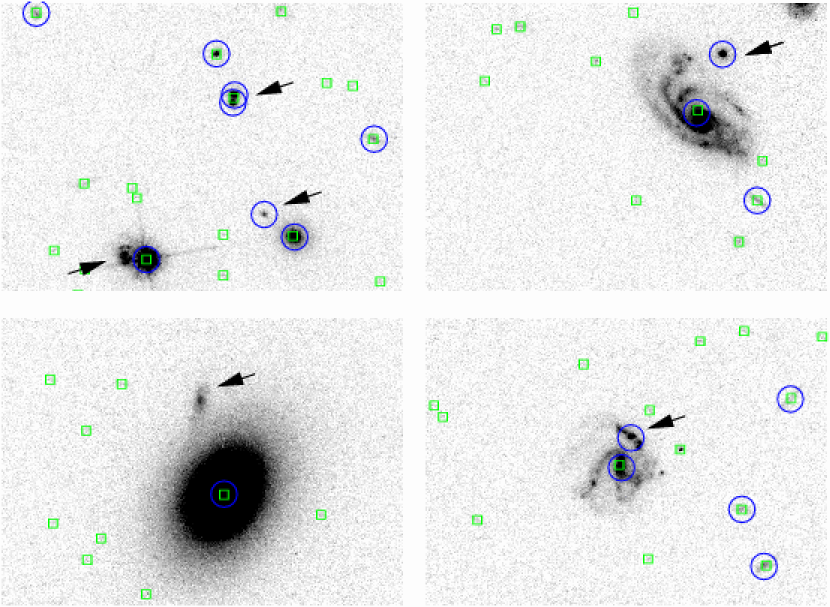
Figure 3: This figure illustrates the difficulty of correctly deblending close pairs while keeping patchy spirals with strong star forming regions intact. Squares indicate detections from the faint step and circles indicate detections from the bright step. The top two panels show three objects that are not detected or incorrectly deblended by the faint step but that are picked by two step method. The bottom panel and the arrow towards the star in the upper left panel show that even with this method, a perfect configuration is still difficult to reach.

3.3 Faint Object Detection

In the second step, we configure SExtractor to pick up the small, faint objects, taking care to choose the detection parameters to be less conservative than any subsequent lensing cuts (see $\S$6). min_area is set to 18 pixels (corresponding to a diameter of 1.2 times the FWHM of the PSF) and the detection threshold is one sigma above the background level. As objects detected at this step are smaller, the background estimation can be improved by refining the mesh size of the background map and setting back_size to 100 pixels, or 20 times the diameter of the smallest objects detected. This second catalog is referred to hereafter as $\mathcal{C}_{hot}$.

3.4 Merging the Two Samples

The final catalog is obtained by merging the detections from $\mathcal{C}_{cold}$ and $\mathcal{C}_{hot}$, keeping all objects in $\mathcal{C}_{cold}$ and only the objects from $\mathcal{C}_{hot}$ not detected in $\mathcal{C}_{cold}$. To determine which objects to discard from $\mathcal{C}_{hot}$, we use the segmentation maps created during the bright detection step. To begin with, we enlarge the flagged areas in these segmentation maps by approximately 20 pixels (0.6$\arcsec$). We then discard all objects from $\mathcal{C}_{hot}$ for which the central pixel lies within a flagged area of these maps. Thus, we remove duplicate detections and create a mask around all bright objects, immediately cleaning the catalog of a certain number of spurious detections. By a visual inspection of the data, we estimate that this method solves about half of the deblending problems that we observe (excluding the low surface brightness galaxies). The final catalog of raw SExtractor detections $\mathcal{C}_{1}$ contains 1.8 million objects in total (see Table 2).

Table 2: Sumary of the construction of the ACS lensing catalog

Catalog of raw SExtractor detections: $\mathcal{C}_{1}$	Number	Percent of $\mathcal{C}_{1}$
Total number of objects in $\mathcal{C}_{1}$	1.8 $\times 10^{6}$
Number of Hot (faint) detections	1.6$\times 10^{6}$	88%
Number of Cold (bright) detections	2.2$\times 10^{5}$	12%
Details of the cleaning process	Number	Percent of $\mathcal{C}_{1}$
Number of objects within the noisy border of a tile	3.2$\times 10^{5}$	17%
Number of Hot detections with central pixel in Cold segmentation map	2.0$\times 10^{5}$	11%
Number of objects within automatically defined star masks	2.4$\times 10^{4}$	1%
Number of objects within manually defined masks	4.1$\times 10^{4}$	2%
Number of objects detected more than once in adjacent tiles	6.6$\times 10^{4}$	4%
Catalog cleaned of image defects: $\mathcal{C}_{2}$	Number	Percent of $\mathcal{C}_{2}$
Total number of objects in $\mathcal{C}_{2}$	1.2$\times 10^{6}$
Number of galaxies ($ID=1$)	1.1$\times 10^{6}$	96 %
Number of point sources ($ID=2$)	2.8$\times 10^{4}$	2 %
Number of fake detections ($ID=3$)	1.7 $\times 10^{4}$	2%
ACS galaxies from $\mathcal{C}_{2}$ with $F814W_{AB}<26.5$: $\mathcal{C}_{3}$	Number	Percent of $\mathcal{C}_{3}$
Total number of objects in $\mathcal{C}_{3}$	7.0$\times 10^{5}$
Number of galaxies with a counterpart in the photometric catalog	6.0$\times 10^{5}$	85%
Number of galaxies that have been matched but that are in ground based masks	8.3$\times 10^{4}$	12%
Number of galaxies for which the redshift code did not converge	1.1$\times 10^{4}$	1.7%
Total number of galaxies with accurate photometric redshifts, $\mathcal{C}_{3}$	5.0$\times 10^{5}$	71%
The final COSMOS ACS lensing catalog: $\mathcal{C}_{4}$	Number	Galaxy number density
Total number of galaxies in final lensing catalog	3.9$\times 10^{5}$	66 arcmin2
Number of galaxies with accurate photometric redshifts	2.8$\times 10^{5}$	48 arcmin2

3.5 Cleaning the Catalog

Great care was taken to mask unreliable regions within images and to remove false detections from the catalog, especially those that can mimic a lensing signal. As illustrated in Figure 2, an automatic algorithm was developed to define polygonal shaped masks around stars with $F814W<19$ (the limit at which stars saturate in the COSMOS images), with a size scaled by the magnitude of the star. Objects near bright stars or saturated pixels were masked to avoid shape biases due to any background gradient. All the images were then visually inspected. In a few cases the automatic algorithm failed (very saturated stars for which the centroid of the star is widely offset) and the stellar masks were corrected by hand. Other contaminated regions of the images were also masked out, including reflection ghosts, asteroids, and satellite trails. Astronomical sources such as HII regions around bright galaxies, stellar clusters, and nearby dwarf galaxies, were also flagged and removed from the lensing catalog.

Objects with double entries in the catalog (from the overlap between adjacent images) are identified and the counterpart with the highest SExtractor flag (indicating a poor detection) is discarded, leaving a catalog of unique objects. However, the duplicated objects from overlapping regions are a valuable asset for consistency checks and are used, for example, to check the galaxy shape measurement error (see $\S$7 and Figure 17).

The final clean catalog ($\mathcal{C}_{2}$) is free of spurious or duplicate detections and contains 1.2 million sources in total (see Table 2).

3.6 Star-Galaxy Classification

The correct identification of stars has two implications for the lensing analysis. First, bright stars are useful for PSF modelling and second, stars must be correctly identified in order to apply our automatic masking algorithm of diffraction spikes. A robust star-galaxy classification is thus necessary.

SExtractor produces a continuous stellar classification index parameter ranging from 0 (extended sources) to 1 (point sources). This index has two drawbacks: first the definition of the dividing line is ambiguous and second, the neural-network classifier used by SExtractor is trained with ground-based images and is therefore only valid for a sample of profiles similar to the original training set. With space-based images, this index becomes difficult to interpret, as illustrated in Figure 4 which depicts our star selection (described below) within the class_star/mag_auto plane.

We therefore test two alternative methods to classify point sources and galaxies, one based on the SExtractor parameter mu_max (peak surface brightness above the background level) and the other based on the half-light radius, Rhl (e.g., Peterson et al., 1979; Bardeau et al., 2005). Both methods are motivated by the fact that the light distribution of a point source scales with magnitude. Point sources therefore occupy a well-defined locus in a mu_max/mag_auto or a Rhl/mag_auto plane. Figure 5 shows how we can use this property to define stars (ID=2) and galaxies (ID=1) reliably up to a magnitude of $F814W\sim 25$. At fainter levels, the classification begins to break down and the point sources become indistinguishable from the small galaxies. We find that the two methods agree very well, within 1% at magnitudes less than $F814W=24$ and within 2% at magnitudes less than $F814W=25$. The small difference arises mainly from a misclassification of objects by the Rhl method because of the presence of a close pair that distorts the estimation of Rhl. Overall, the mu_max method proved to be more robust and has the advantage of a tighter correlation of the stellar locus and a clear break indicating the magnitude at which the stars saturate ($\textsc{mag\_auto}\sim 19$). Moreover, with this method, a surface brightness cut at the faint end of the stellar sample is trivial to implement (at faint magnitudes, the catalog is surface brightness limited). The performance of this star galaxy separation scheme will be analyzed in more detail in $\S$ 4.1.

Using the mu_max method, we also define a set of objects that are more sharply peaked than the PSF, which is obviously non-physical. A visual inspection finds that these objects are mainly artifacts, hot pixels, and residual cosmic rays. We flag these spurious objects in our catalog (ID=3) and remove them for the lensing analysis.

Averaging over the COSMOS field, we find $\sim 15$ stars per pointing with $19\leq\textsc{mag\_auto}\leq 23$. This is an insufficient number to model the PSF in individual images using standard interpolation techniques. However, it is a sufficient number to identify the PSF pattern of each exposure given a finite set of recurring patterns (see $\S$ 5.1 and Rhodes et al. (2007) for further details).

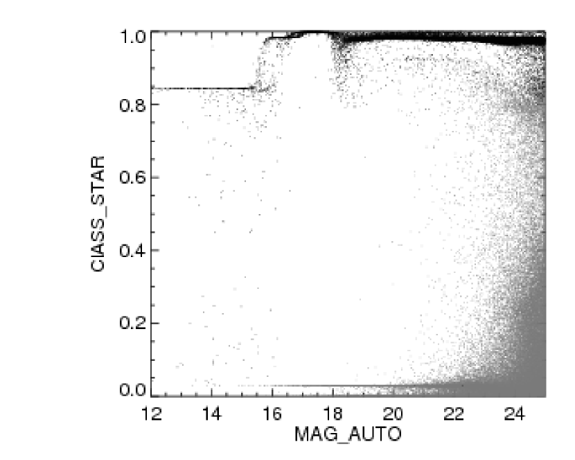
Figure 4: The SExtractor stellar index (class_star) for our point source selection based on the peak surface brightness of objects. Grey points show the corresponding galaxy sample. A point source selection of the form $\textsc{class\_star}>0.8$ for example, will miss a certain number of bright stars ($F814W<17$) and will grossly misclassify compact galaxies at $22<F814W<25$.

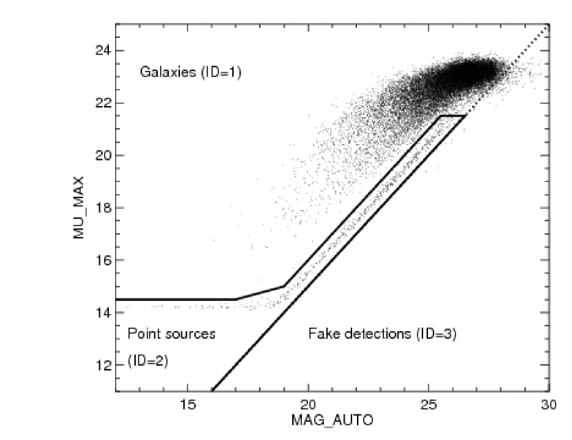
Figure 5: Classification of point sources, galaxies and artifacts within the mu_max/ mag_auto plane. Point sources follow the PSF and are delimited by the solid region. Objects that are more sharply peaked than the PSF are contained in the dashed region and are considered to be artifacts. For clarity, only a 2% random selection of all objects are included in this plot.

3.7 Photometric Redshifts

In addition to the ACS/WFC ($F814W$) imaging, the COSMOS field has been imaged with Subaru Suprime-Cam ($B_{j}$,$V_{j}$,$g+$,$r+$,$i+$, $z+$,$NB816$), the Canada-French Hawaii Telescope (CFHT) ($u*,i*$) and the KPNO/CTIO ($Ks$). Details of the ground-based observations and the data reduction are presented in Capak et al. (2007) and Taniguchi et al. (2007). Other observations were taken in the UV with GALEX, in the X-ray with XMM-Newton and in the radio with VLA, CSO and IRAM. Yet more observations are underway including intermediate and narrow-band imaging with Subaru Suprime-Cam, deep Infrared imaging covering 1.0-2.2 microns (WIRCam/CFHT, WFCAM/UKIRT and ULBcam/UH2.2), and observations with space-based facilities including Chandra and Spitzer Space Telescopes. This extensive multi-wavelength data-set is a key component to COSMOS weak lensing measurements because it allows us to accurately measure the COSMOS redshift distribution, to separate foreground and background structures, and to remove contamination from intrinsic galaxy alignments (Heymans & Heavens, 2003) and shear-ellipticity correlations (King, 2005).

Photometric redshifts were determined by the COSMOS photometric redshift code with a Bayesian prior based on luminosity functions and allowing for internal extinction (Mobasher et al., 2007). For each galaxy, the entire probability distribution $P(z)$, the most likely redshift and a confidence level for that redshift is calculated. The knowledge of the full $P(z)$ allows us to apply weight to galaxies in weak lensing measurements according to the uncertainty in their measured redshift. The accuracy of the photometric redshifts are estimated based on extensive simulations and by comparison with a sample of 958 galaxies with spectroscopic redshifts measured by the ESO/VIMOS instrument as part as the zCOSMOS program (Lilly et al., 2007). Both the luminosity prior and the extinction corrections have been shown to improve the accuracy of the photometric redshifts when compared to the spectroscopic sample. The accuracy of the current photometric redshifts down to $F814W\sim 22.5$ is:

$$\sigma_{\Delta z}/(1+z_{s})=0.031$$ (1)

with $\eta=1.0\%$ of catastrophic errors, defined as $\Delta z/(1+z_{s})>0.15$. This relation scales with magnitude in a similar fashion to Wolf et al. (2004). The accuracy of the photometric redshifts will continue to improve as more data become available (in particular the deeper $u*$, $J$, $K$, Spitzer and Subaru narrow band data).

The COSMOS optical and near infrared catalog (Capak et al., 2007) provides multi-band photometry for 89% of the COSMOS ACS/WFC galaxies. As demonstrated by Figure 6, the remaining 11% of the galaxies for which we lack multi-wavelength information (and therefore photometric redshifts), are the small galaxies that cannot be detected by the ground based imaging. In effect, although the SUBARU data is deeper for sources 1″ in diameter, the ACS/WFC imaging will do a better job at detecting anything smaller. Because we apply a size cut to the the final lensing catalog however (see $\S$ 6), many of these small galaxies will be discarded from the final analysis. In total, after removing the galaxies with unreliable multi-band photometry (because they are masked out in the ground-based data) as well as those for which the photometric redshift code failed to converge, 76% of the galaxies in the COSMOS ACS/WFC lensing catalog ($F814W<26$) have photometric redshifts (See Figure 6). For further discussions on the photometric redshifts and the COSMOS redshift distribution, see $\S$ 4.3.

Figure 6: In the upper panel, the number counts of galaxies that have been correctly matched to the ground based catalog (dotted line) are compared to the total number counts (solid line). The dashed line indicates galaxies for which we consider the photometric redshift to be reliable. The difference between these two curves is primarily due to larger masked areas in the ground-based data than in the ACS imaging. In the lower panel, the sizes of galaxies within the ACS catalog (solid line) are compared to the sizes of those that have been matched with the ground based catalog (dashed line). The objects for which we do not have multi-band photometry are small galaxies that are detected with ACS but not with ground based imaging (seeing $\sim 1\arcsec$). The vertical dashed line shows the approximate size cut that we make in the final lensing catalog.

3.8 Noise Properties

The drizzling process introduces pattern-dependent correlations between neighboring pixels and can artificially reduce the noise levels in co-added images. Noise and error estimates derived from drizzled images will thus tend to underestimate the true noise levels of the image. One should in theory take into account the exact covariance matrix of the noise in order to derive error estimates for drizzled images. For our purposes, however, a simple scaling of the noise level is each pixel by the same constant factor is sufficient. The scaling factor that we adopt, $F_{A}$, has been derived for MultiDrizzled images by Casertano et al. (2000). In principle $F_{A}$ is size dependent but converges rapidly with increasing size toward an asymptotic value given by:

$$\sqrt{F_{A}}=\left\{\begin{array}[]{ll}(s/p)(1-s/(3p))&(s<p)\\ (1-p/(3s))&(p<s)\end{array}\right.$$ (2)

where $p$ and $s$ are respectively the pixfrac and the scale configuration parameters of MultiDrizzle. For the purpose of this paper, we assume $F_{A}$ to be constant and equal to $F_{A}\sim 0.316$ ($p=0.8$ and $s=0.6$). By assuming a constant corrective factor regardless of size, we make less than a 10% error on the noise estimation of the smallest objects detected.

As implemented by SExtractor, the formulas for the flux and magnitude uncertainties (for both auto and the iso quantities) are given by:

$$\textsc{flux\_err}=\sqrt{A\sigma^{2}+F/g}$$ (3)

$$\textsc{mag\_err}=\frac{2.5}{\ln 10}\frac{\textsc{flux\_err}}{F}$$ (4)

where $A$ is the area (in pixels) over which the flux $F$ (in ADU) is summed and $g$ is the detector gain. To correct the magnitude and flux errors reported by SExtractor for the correlated noise, we replace $\sigma$, the standard deviation of the noise (in ADU) estimated by SExtractor, by $\sigma/\sqrt{F_{A}}$ within the above equations. The significance of a COSMOS detection, after this correction is applied, is defined as $\textsc{s/n}=\textsc{flux\_auto}/\textsc{fluxerr\_auto}$ (see Figure 7).

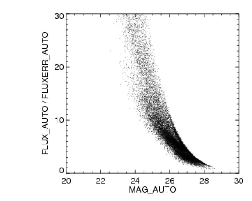
Figure 7: The significance of COSMOS detections defined as flux_auto/fluxerr_auto where fluxerr_auto has been corrected for correlated noise.

4 Quality Assessment of the ACS Catalog

4.1 Galaxy and Stellar Counts

The same mu_max parameter used to classify stars and galaxies can also be used as an indication of the background level and the depth of the data. For each image i we calculate the mode $m_{i}$ of the mu_max parameter. We then divide the $m_{i}$ into two bins according to the angle of the telescope with the Sun at the moment of the pointing. The histogram of $m_{i}$ (Figure 8) for these two bins reveals that the depth of the data is bimodal depending on whether the angle of the sun is less or greater than a critical angle of 70 deg. This is visually evident when we inspect the density map of the very faint objects (Figure 8). 96 pointings out of 575 have a Sun angle less than the critical value making them slightly shallower than the average.

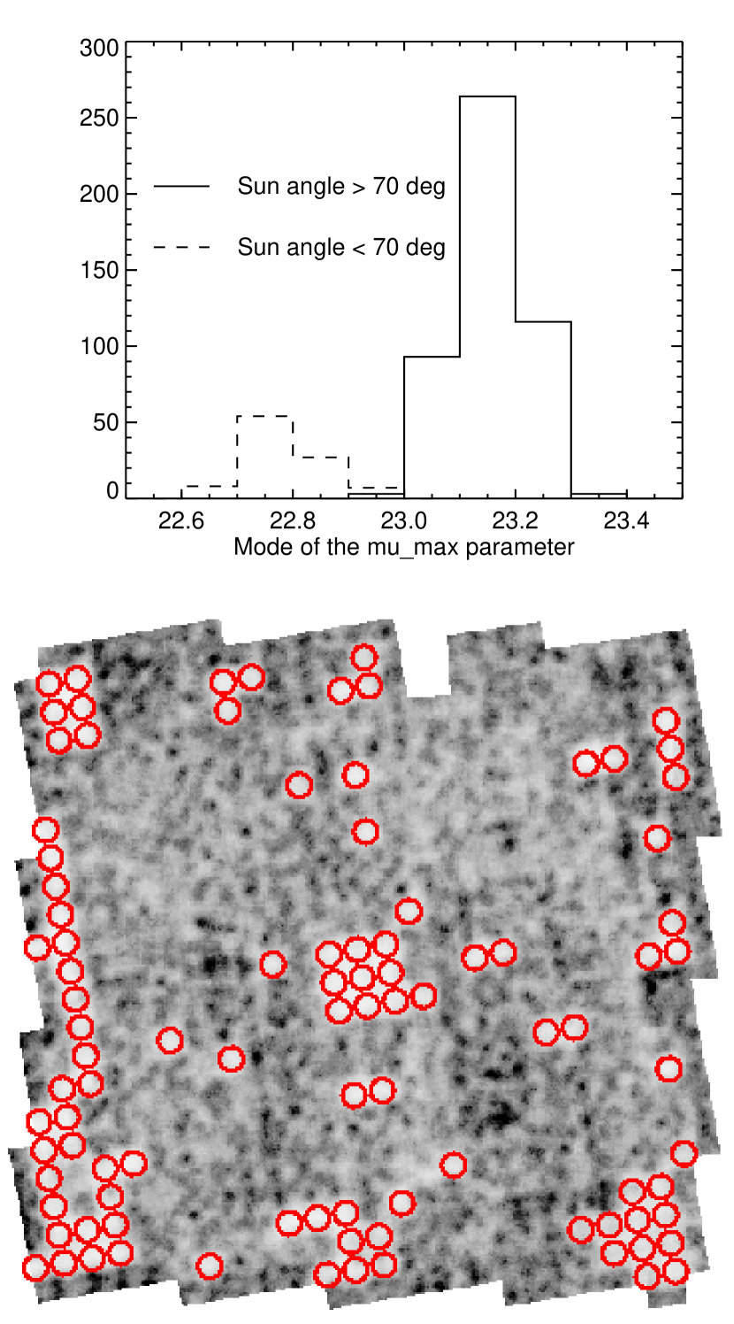
Figure 8: The top panel shows the histogram of $m_{i}$ (mode of the mu_max parameter for each image) demonstrating that images with a sun angle less than 70 degrees are not quite as deep as images with a sun angle greater than 70 degrees. The bottom panel shows the density of faint objects ($27<F814W<28$) within the COSMOS field. The red circles indicate the pointings for which the angle with the sun is less than 70 degrees.

The number counts serve as a check of the approximate photometric calibration and the depth of the data. Figure 9 shows the counts for galaxies and stars compared to the reported HDF F814W counts (Williams et al., 1996). The magnitudes are given in the AB-system. Stars have been subtracted from the galaxy counts up to $F814W=25$. At fainter magnitudes their contribution is negligible. We plot raw number counts only, i.e. we do not correct for incompleteness at the faint end. To facilitate comparisons with other surveys, we fit the galaxy counts between $F814W=20$ and $F814W=26$, to an exponential of the form $N=B\times 10^{A\times mag}$ where N has units of number degree^-2 0.5 mag^-1. For the deeper set of images (sun angle $>$ 70 degrees), we find $A=0.332$ and $log_{10}(B)=-3.543$. The raw galaxy and stellar number counts are provided in Table 3.

We also fit the stellar counts to models as shown in Figure 9. The star count predictions have been done using the Besançon model of the Galaxy (Robin et al., 2003, 2004) and are described in detail in (Robin et al., 2007). By extrapolating the stellar number counts, we estimate that the galaxy catalog has less than a 3% contamination from stars at magnitudes greater than 25. The fit to stellar models is excellent between $F814W=20$ and $F814W=25$, and at magnitudes less than 19, we visually inspect the catalog to check that the star selection is correct to within 0.5%. This small error arises mainly from false detections by SExtractor of the diffraction spikes of bright, saturated stars.

Table 3: Cosmos F814W galaxy and stellar number counts

$F814W$	Galaxy density	Stellar density
	$log_{10}(n)$ deg-2 0.5 mag-1	$log_{10}(n)$ deg-2 0.5 mag-1
20.25	3.138 $\pm$ 1.503	2.807 $\pm$ 1.297
20.75	3.323 $\pm$ 1.600	2.865 $\pm$ 1.329
21.25	3.514 $\pm$ 1.691	2.930 $\pm$ 1.361
21.75	3.686 $\pm$ 1.777	2.936 $\pm$ 1.365
22.25	3.853 $\pm$ 1.860	2.981 $\pm$ 1.385
22.75	4.022 $\pm$ 1.945	3.003 $\pm$ 1.401
23.25	4.180 $\pm$ 2.023	3.043 $\pm$ 1.414
23.75	4.352 $\pm$ 2.110	3.081 $\pm$ 1.437
24.25	4.523 $\pm$ 2.196	3.143 $\pm$ 1.463
24.75	4.682 $\pm$ 2.275	3.206 $\pm$ 1.493
25.25	4.814 $\pm$ 2.340	$\cdots$
25.75	4.956 $\pm$ 2.412	$\cdots$

.

Note. — Galaxy counts are derived for the 479 images with a sunangle greater than 70 degrees. Magnitudes are the SExtractor mag_auto

Figure 9: The top panel shows the galaxy and stellar number counts as compared to the HDF. The dashed curve corresponds to images with a sun-angle of less than 70 degrees and the solid curve corresponds to images with a sun-angle greater than 70 degrees. Poisson error bars are also indicated but are very small. The bottom panel shows the point source selection for the catalog compared to stellar models computed from evolutionary tracks and constrained by local Hipparcos data.

4.2 Completeness

The probability that a galaxy enters our catalog will depend on its size and surface brightness profile. To quantify the completeness and detection limits of our SExtractor configuration, we insert fake objects with a Gaussian profile of varying FWHM and total magnitude into empty regions of an ACS image and test how well these objects can be recovered with our pipeline. Each artificial source was considered to be correctly detected if its centroid was within 10 pixels and the mag_auto parameter was within 0.5 mag of the input value. From this analysis, we determine our completeness as a function of magnitude and FWHM and the results are shown in Figure 10. The completeness is about 90% for objects with a FWHM of 0.2″ at F814W=26.6. These values should only be used as a rough estimate however, as we do not actually model galaxies, but use a simple Gaussian profile for artificial objects.

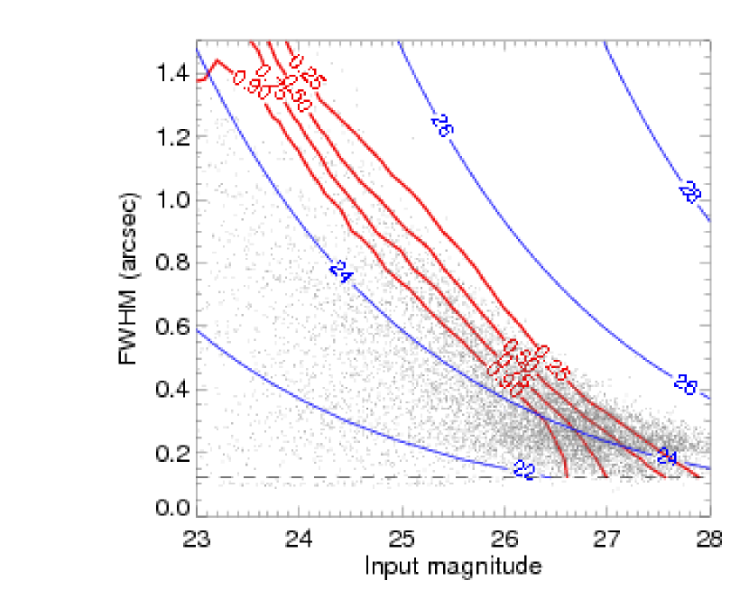
Figure 10: Completeness of the COSMOS F814W catalog as a function of total magnitude and FWHM determined by inserting fake objects into an ACS image. The thick contours show the percentage of fake objects recovered by SExtractor. The thin contours are the lines of constant surface brightness, in units of mag arcsec^-2, assuming a Gaussian profile. The grey points represent a random sample of objects from the COSMOS catalog plotted as a function of mag_auto and fwhm_image. The dashed horizontal line indicates the size of the ACS PSF. Note that the simulations only consider objects with Gaussian profiles whereas in reality, the COSMOS objects exhibit a wide variety of profiles.

4.3 The COSMOS Redshift Distribution

The estimation of the redshifts of galaxies is the major astrophysical uncertainty inherent to weak lensing methods. To first approximation, cosmic shear and tomography are mainly sensitive to the median redshift of the sources while galaxy-galaxy lensing benefits greatly from the knowledge of precise spectroscopic redshifts for the foreground lenses (Kleinheinrich et al., 2005). With the depth and area coverage of COSMOS, we surpass the current capability for complete spectroscopic follow-up. For most forthcoming weak lensing surveys, this will also be the case, hence the importance of the photometric redshift technique to measure redshifts for a majority of the galaxies, to and beyond today’s spectroscopic limits (Ilbert et al., 2006). COSMOS presents a unique advantage, in terms of current weak lensing surveys, of a prodigious multi-wavelength follow-up combined with the planned measurement of $\sim 50000$ spectroscopic redshifts by the ongoing zCOSMOS program (Lilly et al., 2007). Upon completion, this data set will provide the COSMOS lensing catalog with accurate photometric redshifts and will be vital for refining and improving the photometric technique in preparation for forthcoming weak lensing surveys. We present here a first analysis of the COSMOS redshift distribution. A more detailed study of the systematic trends in the photometric redshifts and of their effects on the redshift distribution is beyond the scope of this paper and will be addressed elsewhere when more data becomes available. For the purposes of this paper, we adopt the magnitude dependent parametrization of the redshift distribution, common to many other weak lensing studies as given by Baugh & Efstathiou (1993),

$$\left\{\begin{array}[]{ll}n(z,mag)\propto z^{2}\exp[-\frac{z}{z_{o}(mag)}^{1.5}]\\ z_{0}(mag)=\frac{z_{m}(mag)}{1.412}\end{array}\right.$$ (5)

where $z_{m}$ is the median redshift of the survey as a function of magnitude. We calculate $z_{m}$ for the COSMOS ACS data by bins of $\Delta F814W=0.25$ for $20<F814W<24$ and derive the best linear fit to $z_{m}$, given by:

$$z_{m}=(0.18\pm 0.01)\times F814W-(3.3\pm 0.2)$$ (6)

The majority of the galaxies for which we have no redshift estimate at $F814W<24$ are those in masked regions and their exclusion from this derivation do not affect this results. At $F814W<24$, our redshift incompleteness is less than $4\%$ and the dominant source of error is the photometric redshift uncertainty expressed previously in Equation 1. We note that a significant number of galaxies fainter then this limit do have photometric redshifts. The fact that these galaxies represent a statistically incomplete sample, does not matter for some applications. For example, these additional galaxies are used in the cosmic shear measurement by Massey et al. (2007).

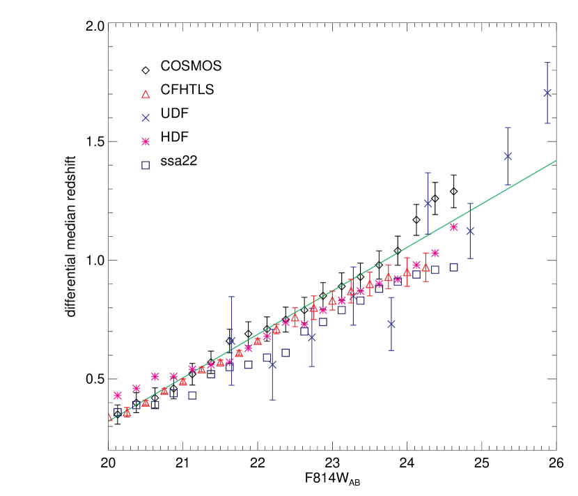
Figure 11: Median redshift of COSMOS compared to various photometric redshift surveys. For clarity, error bars are only shown for the COSMOS, CFHTLS and UDF surveys

Table 4: Present date photometric redshift surveys

Survey	Area	Imaging data	Calibration spectra	Technique
COSMOS	1.67 deg2	$B_{j},V_{j},g+,r+,i+,z+,NB816,u*,i*,Ks$	958	COSMOS/BPZ
UDF	11.97 arcmin2	$B,V,i^{\prime},z^{\prime},J$ $H$	76	BPZ
CFHTLS	3.2 deg2	$u*,g^{\prime},r^{\prime},i^{\prime},z^{\prime},J,K$	2867	Le Phare
H-HDF-N	0.2 deg2	$U_{j},B_{j},V_{j},R_{c},I_{c},Z^{+},HK^{\prime}$	2149	BPZ
SSA22	0.2 deg2	$U^{*}_{j},B_{j},V_{j},R_{c},I_{c},z^{+},J,H,K,HK^{\prime}$	452	BPZ

In Figure 11, we compare the median redshift of COSMOS to the UDF survey (Coe et al., 2006), the CFHTLS survey (Ilbert et al., 2006), the H-HDF-N survey (Capak et al., 2004) and SSA22 (Hu et al. 2004, Capak et al. 2004). Table 4 is a summary of the data and the methods employed by these different photometric redshift surveys. All photometric redshifts have been computed with a Bayesian prior based on luminosity functions. The agreement that we see between the various surveys at $z<1$ is quite remarkable. At $z>1$ however, the scatter in Figure 11 indicates the limits of current photometric techniques. Further simulations are clearly necessary in order to understand the biases introduced in the redshift distribution at $z>1$. Although we reserve a full discussion for a future paper, we can already highlight some of the issues at hand.

The photometric redshift technique relies on detecting and measuring the strength of broad spectral features. These same features are used by color selection techniques to select objects at specific redshifts. The key features are the 4000Å break, the Lyman break at 912Å,̃ Lyman absorption at 1216Å,̃ and coronal line absorption between 1500-2500Å (see Adelburger et. al. 2005). Photometric redshifts are very robust if one or more of these features are detectable in the available data. However, at faint magnitudes the photometric errors and detection limits are often too large to constrain these features.

For example, problems arise for COSMOS between $1.5<z<3.2$ where the measurable features, the 4000Å break, and the coronal line absorption features, are difficult to detect. Indeed, at these redshifts, the 4000Å break is well into the IR where it is difficult to obtain deep data. A typical object at $z\simeq 2$ will be $\sim 1.4$ magnitudes fainter at $I$ than $K$. This means objects fainter than $F814W>23.5$ are not constrained by the present $K$-band data. At the other end of the spectrum the coronal absorption feature has a typical strength of $\sim 0.15$ magnitudes, which requires a $25\sigma$ detection in $u^{*}$ to accurately differentiate from a similar break in $z<0.5$ galaxies. With the present $u^{*}$ data, this corresponds to objects brighter than $F814W<24.5$ for typical galaxies.

In conclusion, the high redshift tail of the COSMOS redshift distribution will be more accurately determined with the forthcoming NIR data and the future deep zCOSMOS spectroscopy which specifically targets the $1.5<z<3$ region and will allow proper calibration down to $F814W\sim 24$. A more detailed analysis of the photometric redshifts will be conducted once the new data is available.

5 PSF Correction and Shear Measurement

In this section, we measure the shapes of galaxies and correct them for the convolution with the telescope’s PSF and for other instrumental effects. For each galaxy, we construct an unbiased local estimator of the shear and derive the associated measurement error.

5.1 PSF Modelling

The ACS/WFC PSF is not as stable as one might naively hope from a space-based camera. As shown in Rhodes et al. (2007), gradual changes to both the size and the ellipticity pattern of the PSF due to telescope “breathing”, causes the PSF to change considerably on timescales of weeks. The long period of time over which the COSMOS field was observed forces us to take account of these variations (see Figure 1). Although other strategies have been demonstrated successfully for observations conducted on a shorter time span, it would be inappropriate for us to assume, like Lombardi et al. (2005) or Jee et al. (2005), that the PSF is constant or even, like Heymans et al. (2005), that the focus is piecewise constant.

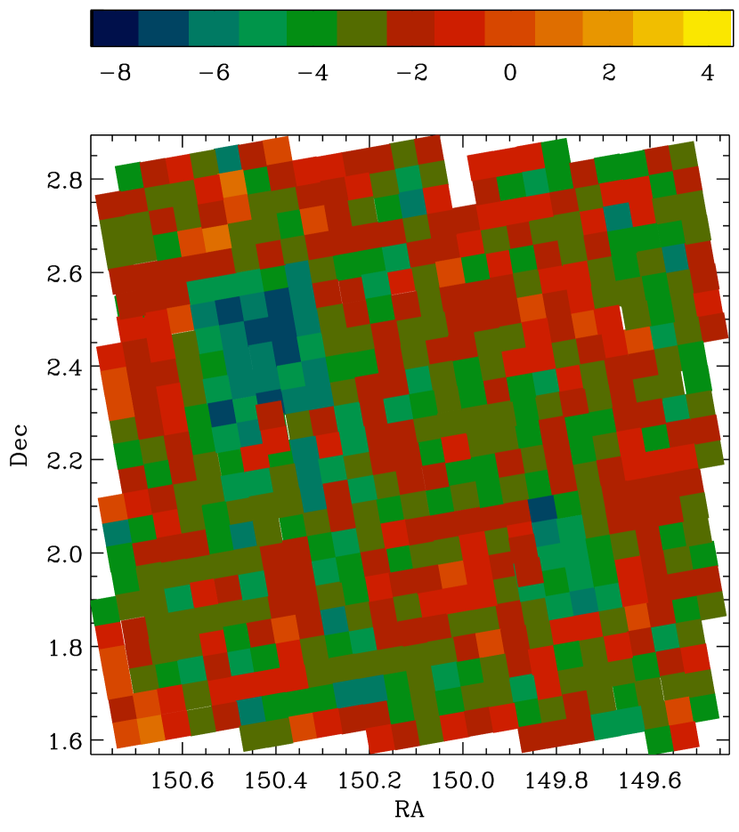
Figure 12: Adopted PSF model across the survey. The colors correspond to deviations in the apparent focus of the telescope away from nominal ($\mu m$). These are caused by expansion and contraction of the HST due to thermal variations. Note that the focus values are clustered and not randomly distributed. See Rhodes et al. 2007 for more details about the PSF pattern at particular focus positions.

Fortunately, most of the PSF variation can be ascribed to a single physical parameter. Thermal expansions and contractions of HST alter the distance between the primary and secondary mirrors. As the “effective focus” deviates from nominal, the PSF becomes larger and more elliptical, with the direction of elongation depending upon the position above or below nominal focus (c.f. Krist, 2005). The thermal load on HST is constantly changing, in a complicated way, as it passes in and out of the shadow of the Earth and is rotated to different pointings.

As described in Rhodes et al. (2007), we have modified version 6.3 of the TinyTim ray-tracing program (Krist and Hook 2004) to create a grid of model PSF images, at varying focus offsets. By comparing the ellipticity of $\sim 20$ stars in each image to these, we can determine the image’s effective focus. Tests of this algorithm on ACS/WFC images of dense stellar fields confirm that the best-fit effective focus can be repeatably determined from a random sample of ten stars brighter than $F814W=23$ with an rms error less than $1\mu$m. The effective focus of the COSMOS images are shown in Figure 12. An alternative correction scheme based on PSF models constructed from dense stellar fields has also been suggested by Schrabback et al. (2006).

Once images have been grouped by their effective focus position, we can combine the few stars in each image into one large catalog. We interpolate the PSF model parameters using a polynomial fit (of order $3\times 2\times 2$ in each CCD separately), in the usual weak lensing fashion (c.f. Massey et al., 2002). See Rhodes et al. (2007) for more details concerning the PSF modelling scheme.

5.2 Galaxy Shape Measurement

We use the shape measurement method developed for space-based imaging by Rhodes et al. (2000, hereafter RRG). The RRG method has been optimized for space-based images with small PSFs and has previously been used on weak lensing analyses of WFPC2 and STIS data (Rhodes et al., 2001; Refregier et al., 2002; Rhodes et al., 2004). In a manner similar to the common “KSB” method (Kaiser et al., 1995), RRG measures the second and fourth order Gaussian-weighted moments of each galaxy:

$$I_{ij}=\frac{\sum wIx_{i}x_{j}}{\sum wI},$$ (7)

$$I_{ijkl}=\frac{\sum wIx_{i}x_{j}x_{k}x_{l}}{\sum wI}.$$ (8)

The sum is over all pixels, $w$ is the size of the Gaussian weight function, $I$ is the pixel intensity, and the $x_{i}$ coordinates are measured in pixels. The Gaussian weight function is necessary to suppress divergent sky noise contributions in the measurement of the quadripole moments. The RRG method is well-suited to the small, diffraction-limited PSF obtained from space, because it decreases the noise on the shear estimators by correcting each moment for the PSF linearly, and only dividing them to form an ellipticity at the last possible moment.

After the moments have been corrected for the PSF, an ellipticity $\varepsilon=(e_{1},e_{2})$ and size measure, $d$, are calculated for each galaxy:

$$e_{1}=\frac{I_{xx}-I_{yy}}{I_{xx}+I_{yy}},$$ (9)

$$e_{2}=\frac{2I_{xy}}{I_{xx}+I_{yy}},$$ (10)

$$d=\sqrt{\frac{(I_{xx}+I_{yy})}{2}}.$$ (11)

Note that the $d$ parameter is a measure of galaxy size but that its value will depend on the choice of the width of the Gaussian weight function, $w$.

5.3 Shear Measurement

The estimator $\varepsilon=(e_{1},e_{2})$ is not yet a shear estimator, because it does not respond linearly to changes in shear. It must first be normalized by a shear susceptibility factor (also known as the “shear polarizability”),

$$\tilde{\gamma}=\{\tilde{\gamma}_{1},\tilde{\gamma}_{2}\}=\frac{\varepsilon}{G}~{},$$ (12)

where the shear susceptibility factor, $G$, is measured from moments of the global distribution of $\varepsilon$ and other, higher order shape parameters (see equation 28 in Rhodes et al., 2000). The RRG formalism does not allow for $G$ to be calculated for any individual galaxy. However, $G$ can be calculated for an ensemble of galaxies by averaging over a population’s shape moments. Previous incarnations of RRG that have been used to measure cosmic shear (Rhodes et al., 2001; Refregier et al., 2002; Rhodes et al., 2004), have made use of a single value of $G$ for the entire survey. Adopting this approach for the COSMOS data would yield a value of $G=1.13$. However, the Shear TEsting Program (Massey et al., 2007) showed that $G$ can vary significantly as a function of object flux, whether this be due to evolution in galaxy morphologies as a function of redshift, or noise in the wings of faint galaxies that simply impedes the measurement of their radial profiles and higher order moments. An increase in shear susceptibility with object $S{\rm/}N$ has also been seen in KSB-type analyses (Massey et al., 2004a).

Our tests have confirmed that a constant value would be insufficiently precise for a survey the size of COSMOS, and would particularly affect the kind of 3D analysis for which COSMOS is so well-suited. We therefore calculate $G$ from the COSMOS data in bins of $S{\rm/}N$ (see Figure 13). Simulated images of the COSMOS data are created using the shapelets-based method of Massey et al. (2004b) (see $\S$5.4). The variations of $G$ as a function of $S{\rm/}N$ are apparent in the COSMOS data are well reproduced by the simulated data. For COSMOS galaxies, we find that variations in $G$ as a function of $S{\rm/}N$ are well-fit by

$$G=1.125+0.04\arctan\left(\frac{S{\rm/}N-17}{4}\right).$$ (13)

Adopting the above model, we derive $G$ for each galaxy as a function of $S{\rm/}N$.

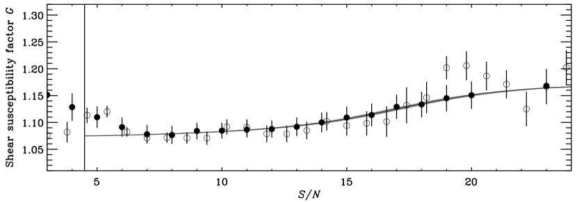
Figure 13: Interpolation of the shear susceptibility factor $G$. The solid circles show $G$, calculated in bins of $S{\rm/}N$, for the COSMOS data. The open circles show the same for the simulated COSMOS images. The solid line shows the shear susceptibility model adopted for the data.

5.4 Calibration via Simulated Images

Using the shapelets-based method of Massey et al. (2004b), we have created simulated images with the same depth, noise properties, PSF, and galaxy morphology distribution as the real COSMOS data. A known shear signal was applied to the images, which we have then attempted to measure using the same pipeline as the data. This exercise is similar to the Shear TEsting Program (STEP; Heymans et al., 2006; Massey et al., 2006) but tailored exclusively to COSMOS.

The simulated COSMOS images are each $4\arcmin\times 4\arcmin$, and contain $\sim 500$ galaxies after applying the same catalog cuts that were applied to the real data (see $\S$6). Simulated galaxy morphologies are based on those observed in the Hubble Deep Fields (Williams et al., 1996, 1998), parametrized as shapelets and randomly rotated/flipped before being sheared. Different input galaxies were used in each simulated image, as if they were pointing to different patches of the sky, to keep them independent. To simplify later analysis, all of the galaxies within an image were sheared by the same amount. A total of 41 images were made, with shears applied in integer steps from $-10\%$ to $+10\%$ in the $\gamma_{1}$ component (while $\gamma_{2}$ was fixed at zero) and similarly for the $\gamma_{2}$ component. The images were then convolved with a model ACS PSF. Again to simplify the analysis, this was a constant PSF obtained from TinyTim. Its $(e_{1},e_{2})$ ellipticity is $(-0.21\%,-2.07\%)\pm(0.14,0.10)$. No stars were included in the simulated images; a separate star field was created, from which the PSF moments could be measured. Noise was added to all of these images, to the same depth as the COSMOS observations, and with a similar (but isotropic) correlation between adjacent pixels to mimic the effects of MultiDrizzle and unresolved background sources.

Figure 14: Calibration of the RRG shear measurement method from simulated COSMOS images containing a known input shear. The measured shear on the y-axis includes the shear calibration factor $C$. Squares show measurements of $\gamma_{1}$, diamonds show measurements of $\gamma_{2}$. The solid line is a linear fit to deviations from the ideal case of $\gamma_{\rm measured}=\gamma_{\rm input}$ for all points. The dashed line is a quadratic fit demonstrating that the curvature terms are negligible.

The recovered shear measurement from the simulated data is presented in Figure 14. We find that, in order to correctly measure the input shear on COSMOS-like images, the RRG method requires an overall calibration factor of $C=(0.86^{+0.07}_{-0.05})^{-1}$, so that

$$\tilde{\gamma}=C\times\frac{\varepsilon}{G}~{}.$$ (14)

The necessity for such calibration factors has long been known in the field (e.g. Bacon et al., 2001; Erben et al., 2001), and is in accord with results from STEP1. STEP2 and Highet al. (2007) suggest that this may be intrinsic with KSB-related methods and, furthermore, that the calibration can vary for the two components of shear. For this reason, we fit each component separately, and use final calibration factors of $C_{1}=(0.80)^{-1}$ for $\tilde{\gamma}_{1}$ and $C_{2}=(0.92)^{-1}$ for $\tilde{\gamma}_{2}$. After this recalibration, Table 5 shows STEP-like estimates of the additive bias $\langle c\rangle$ and the multiplicative bias $\langle m\rangle$ obtained by fitting deviations of the recovered shear from the input shear. Both of these are consistent with ideal shear recovery, although the error on these estimates will be propagated through subsequent analyses.

Linear STEP fit
$\langle c\rangle$	( 2.1 $\pm$	$40.0)\times 10^{-4}$
$c_{1}$	( 5.6 $\pm$	$28.5)\times 10^{-4}$
$c_{2}$	(-1.3 $\pm$	$28.0)\times 10^{-4}$
$\langle m\rangle$	(-0.3 $\pm$	$9.4)\times 10^{-2}$
$m_{1}$	(-12.2 $\pm$	$6.5)\times 10^{-2}$
$m_{2}$	( 11.6 $\pm$	$6.3)\times 10^{-2}$
Quadratic STEP fit
$\langle c\rangle$	(-23.3 $\pm$	$121.8)\times 10^{-4}$
$\langle m\rangle$	( 20.1 $\pm$	$51.5)\times 10^{-2}$
$\langle q\rangle$	-2.84 $\pm$	4.59

Table 5: — Calibration of the RRG shear measurement method on simulated COSMOS images containing a known shear, described using STEP parameters. Figures are supplied after the application of the shear calibration factor.

For the kind of 3D shear analysis for which COSMOS is so well-suited, the simultaneous calibration of shears from an entire population of galaxies is insufficient. Since our companion paper, Massey et al. (2007), is concerned with the growth of the shear signal as a function of redshift, it is crucial that the shear calibration be equally precise for both distant and relatively nearby galaxies. Given that more distant galaxies are fainter and smaller and that the details of the shear measurement depend upon a fixed PSF size, pixel size, and noise level, this requirement is not trivial. We have therefore split the simulated galaxy catalog in half by magnitude (at $F814W=25.4$) and by size (at $d=5.0$ pixels), and repeated the analysis. We find that our shear calibration $\langle m\rangle$ is robust for galaxies of different fluxes within $1\%$ and of different sizes within $4\%$. Redshifts were not available for the simulated galaxies, so a direct split in redshift was not possible. Although this effect is clearly small in the regime of our current measurements, it will be significant in future weak lensing surveys where the error budget will be dominated by systematic uncertainties.

5.5 Error on the Shear Estimator

For each galaxy, the error on the measured shear is estimated using the same method as implemented in the Photo pipeline (Lupton et al., 2001) to analyze data from the Sloan Digital Sky Survey. For each object, we assume that the optimal moments are the same as the moments corresponding to a best fit Gaussian. This formulation allows us to determine the covariance matrix of the moments in the usual way of non-linear least squares. To be precise, we model the image with a 2D elliptical Gaussian model

$$M({\bf x})=\frac{f}{2\pi|Q|^{1/2}}\times$$

$$\exp[-\frac{1}{2}({\bf x-\mu})^{T}Q^{-1}{\bf(x-\mu)}].$$ (15)

This model has six parameters: the flux, $f$, the two centroids, ${\bf\mu}$, and the three moments which form the elements of the symmetric matrix $Q$. These parameters are noted ${p_{l}}$. Next, we derive the $\chi^{2}$ in the usual way

$$\chi^{2}\equiv\frac{1}{\sigma^{2}}\sum_{ij}[M({\bf x_{ij}})-I_{ij}]^{2},$$ (16)

where $\sigma$ is the sky noise level. We can now compute the $6\times 6$ Fisher matrix which is the matrix of the second derivatives of the $\chi^{2}$

$$F_{kl} \equiv \frac{1}{2}\frac{\partial^{2}\chi^{2}}{\partial p_{k}\partial p_{l}}$$

$$= \frac{1}{\sigma^{2}}\sum_{ij}\frac{\partial M({\bf x_{ij}})}{\partial p_{k}}\frac{\partial M({\bf x_{ij}})}{\partial p_{l}}$$

$$- \frac{1}{\sigma^{2}}\sum_{ij}[M({\bf x_{ij}})-I_{ij}]~{}\frac{\partial^{2}M({\bf x_{ij}})}{\partial p_{k}\partial p_{l}}.$$

As is customary, we drop the second term which is proportional to the residuals. This term is usually very small compared to the first. The covariance matrix of the Gaussian parameters are then the inverse of the Fisher matrix. The $3\times 3$ block of the covariance matrix corresponding to the second moments can then be extracted. Because the whole $6\times 6$ matrix was inverted, this correctly marginalizes over centroid errors and other model parameter degeneracies. In this way, it differs from formulas which assume a constant (non-adaptive) weighting function and perfect centroiding.

This Fisher matrix does not depend explicitly on the data; it only depends on the best fit parameters and can be computed analytically. It is simply a function of four numbers: the three second order moments defined in Equation 7 and the signal-to-noise ratio ($f/\sigma$), which can be parametrized by the magnitude error (for example, magerr_auto). Since the flux computed with SExtractor is not exactly equal to $f$ (which would be the best fit Gaussian amplitude) we allow for a single calibration factor and multiply the covariance matrix by this. We calibrate this factor with image simulations and verify that the errors are correctly predicted.

Since the ellipticity components are computed from the moments, the variances of the ellipticity components can be computed by linearly propagating the covariance matrix of the moments. Finally, the two ellipticity components can be shown to be uncorrelated with each other.

6 Final Galaxy Selection

6.1 Lensing Cuts

Estimations of the gravitational shear will be improved by averaging only those galaxies with precise shape measurements on the condition that no ellipticity selection bias is introduced by the “lensing cuts”. We apply strict cuts to the $\mathcal{C}_{2}$ catalog that are designed to extract a sample of resolved galaxies with reliable shape measurements. The resulting catalog is referred to as $\mathcal{C}_{4}$. Our “lensing cuts” are summarized in Table 6 and are based on the four following parameters:

1. The estimated significance of each galaxy detection, where the significance is defined as $\textsc{s/n}=\textsc{flux\_auto}/\textsc{fluxerr\_auto}$,

2. The first order moments, $I_{xx}$ and $I_{yy}$,

3. The total ellipticity, $e=\sqrt{e_{1}^{2}+e_{2}^{2}}$,

4. The galaxy size as defined by the RRG $d$ parameter (see §5.2).

Table 6: Lensing cuts applied to $\mathcal{C}_{2}$

Parameter	Galaxies retained in $\mathcal{C}_{4}$
$I_{xx}$ and $I_{yy}$	Finite $I_{xx}$ and $I_{yy}$
RRG size parameter $d$	$d>3.6$ pixels
Significance	$S/N>4.5$
Total ellipticity $e$	$e<2$

The final size cut is designed to select galaxies with well resolved shapes. Indeed, PSF corrections become increasingly significant as the size of a galaxy approaches that of the PSF and the intrinsic shape of a galaxy becomes more difficult to measure. In COSMOS images, the typical size (as defined by $d$) of a star is about $d\star=2.2$ pixels (0.066″). Our size cut is thus equivalent to selecting galaxies with $d_{g}>1.6\times d\star$. Note that in this section, as well as in all following sections, $d$ has not been corrected for the PSF.

The ellipticity cut at $e<2$ may be surprising given that, by definition, ellipticities are restricted to $e\leq 1$. In reality, however, because of noise, it is possible to measure an ellipticity of $e>1$. Selecting galaxies with $e<1$ could introduce an unwanted ellipticity bias, but, because we are only interested in ensemble averages, an acceptable solution is to cut out only a small number of large outliers ($e>2$).

Note that further cuts may be required for some applications (for example, to isolate only those objects with well-measured photometric redshifts). In addition to these cuts, a galaxy-by-galaxy weighting scheme may also be used to minimize the impact of shape measurement noise.

6.2 Effective Galaxy Number Density

Once the “lensing cuts” have been applied, the $\mathcal{C}_{4}$ catalog contains only those galaxies which are useful for lensing analyses with the COSMOS data. Predictions for future weak lensing surveys based on COSMOS results must consider the “effective number” of galaxies that are actually useful for lensing purposes (and not the number of raw detections). With these considerations in mind, we define the “effective galaxy number density”, $N_{g}(z)$, as the total number of galaxies within $\mathcal{C}_{4}$, per unit area, and with redshifts below a given redshift, $z$. The equivalent quantities as a function of galaxy magnitude and size are $N_{g}(m)$ and $N_{g}(d)$. For each galaxy, the SExtractor mag_auto parameter is used to estimate the magnitude and the RRG $d$ parameter is used as an estimate of the size. We also consider the derivatives of $N_{g}(z)$, $N_{g}(m)$, and $N_{g}(d)$ so that:

$$N_{g}(z)=\int_{0}^{z}n_{g}(z^{\prime})dz^{\prime},$$ (17)

$$N_{g}(m)=\int_{20}^{m}n_{g}(m^{\prime})dm^{\prime},$$ (18)

$$N_{g}(d)=\int_{d}^{\infty}n_{g}(d^{\prime})dd^{\prime}.$$ (19)

The total number density of galaxies in $\mathcal{C}_{4}$ is noted as $N_{g}$ and is significantly lower than the number density of detected galaxies. In total, the final lensing catalog $\mathcal{C}_{4}$ contains 3.9$\times 10^{5}$ galaxies with accurate shape measurements and 2.8$\times 10^{5}$ galaxies with both shape and photometric redshift measurements. Table 2 shows a summary of the different steps leading to this catalog. The surveyed area of COSMOS is 1.64 deg² leading to an overall number density of $N_{g}\sim$66 galaxies per arcmin² for the first sample and $\sim$50 for the second. These numbers can be contrasted to a more sparse 15-25 galaxies per arcmin² typically resolved with deep, ground-based surveys. In Figures 15 and 16 we show the effective densities defined above as well as their corresponding derivatives. From these figures, we can draw the following conclusions:

• Over $60\%$ of the COSMOS source galaxies are at redshifts higher than $z=1$. The COSMOS weak lensing data is therefore a powerful probe of the dark matter distribution from $z\sim 1$ to the present day.

• About $18$ galaxies per arcmin^-2 (73%) are discarded when we select only those galaxies with accurate photometric redshifts. The primary cause of this loss are the larger areas masked out in the ground-based data as compared to the ACS data. Future space-based weak lensing surveys could recover the remaining 27% by using space-based, multi-wavelength imaging to derive photometric redshifts.

• The effective number density rises very steeply with decreasing galaxy size; over $50\%$ of our total number of sources have $d<5$ pixels ($0.15$″). The current size cut for the COSMOS data is $d=3.6$ pixels and the size of the ACS PSF is $d\star=2.2$ pixels (0.066″). By pushing this size barrier to even smaller values, future surveys could very quickly obtain much higher effective densities.

Finally, the cuts that we have applied to the COSMOS data (in particular the size cut) are stricter than would be necessary without significant CTE effects that degrade the shape measurements of the faintest galaxies. Next generation space-based missions designed to avoid the problems encountered and identified in COSMOS, as well as future implementations of the COSMOS catalog, will undoubtedly achieve higher effective number densities.

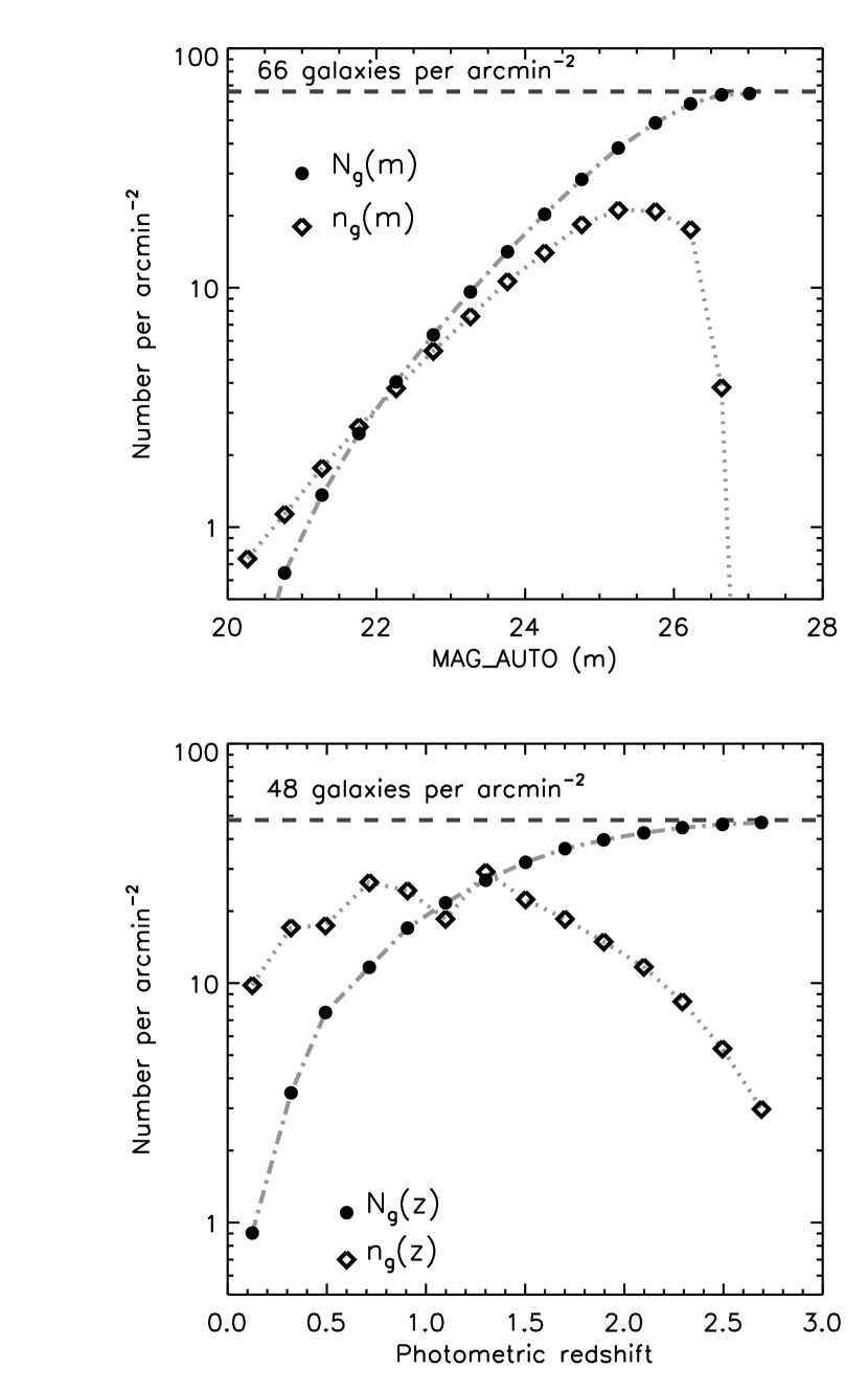
Figure 15: In the upper panel we show the effective number density of galaxies as a function of $F814W$ magnitude. Only resolved galaxies with precise shape measurement are included in these counts. In the lower panel, we show the effective number density of galaxies as a function of redshift. The effective density still evolves sharply after $z>1$ demonstrating that the COSMOS lensing data is a powerful probe of structures at $z<1$.

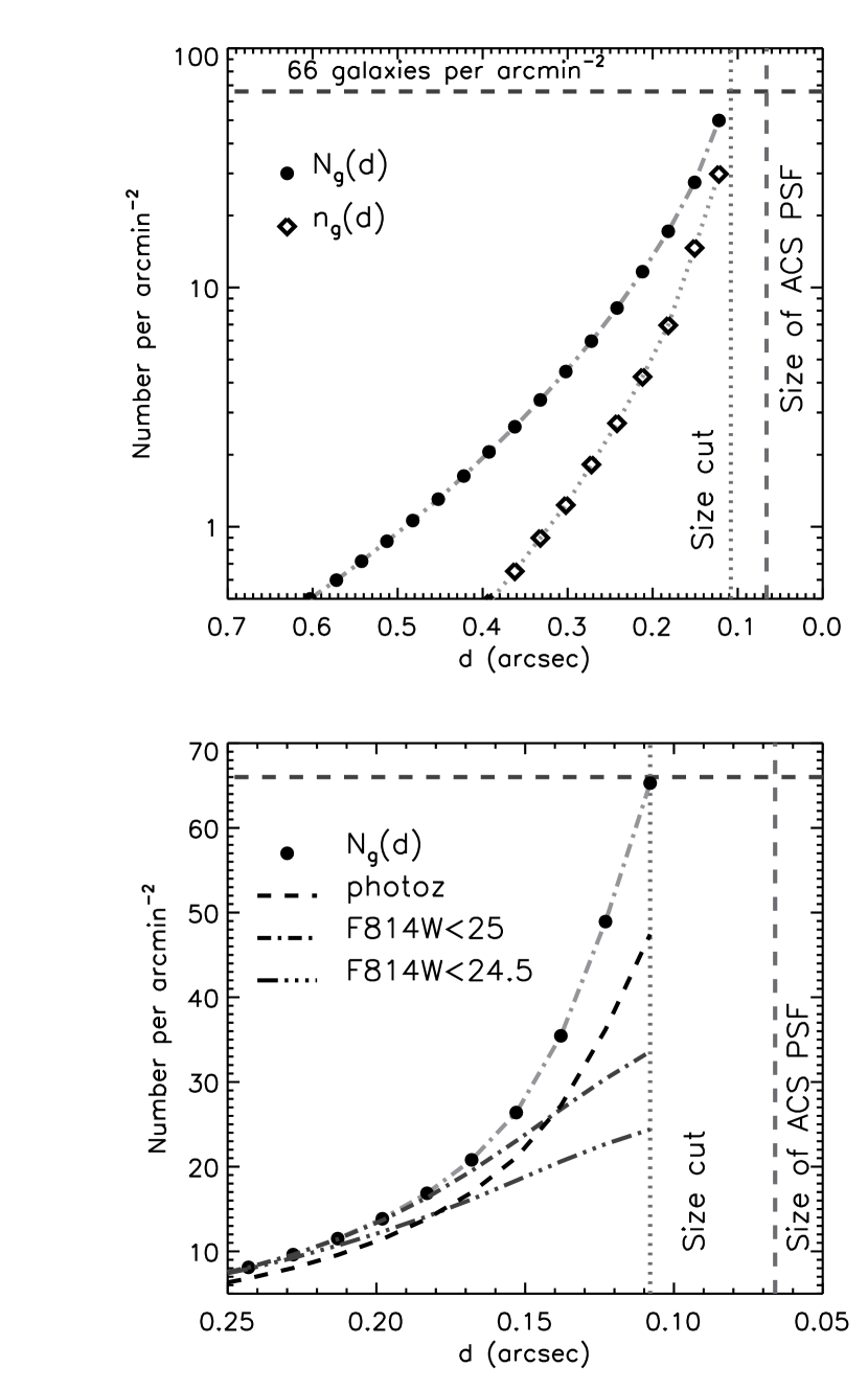
Figure 16: In the upper panel we show the effective number density of galaxies as a function of size. The dotted vertical line indicates the size cut that we make in order to extract galaxies with precise shape measurements. This size cut is such that $d_{g}>1.6\times d\star$. $N_{g}$ rises very sharply as a function of decreasing $d$ demonstrating that small galaxies make up the majority of our lensing sources. The lower panel shows $N_{g}$ for COSMOS galaxies with accurate photometric redshifts and for magnitude cuts of $F814W<25$ and $F814W<24.5$.

7 Intrinsic Shape Noise: a Fundamental Limit to Weak Lensing Measurements

Under the assumption of weak gravitational lensing, a source galaxy with intrinsic shape $\varepsilon_{int}$ and observed ellipticity $\varepsilon_{obs}$ is related to the gravitational lensing induced shear $\gamma$ according to:

$$\varepsilon_{obs}=\varepsilon_{int}+\gamma.$$ (20)

Throughout this paper, the gravitational shear is noted as $\gamma$ whereas $\tilde{\gamma}$ represents our estimator of $\gamma$. The above relationship indicates that galaxies would be ideal tracers of the distortions caused by gravitational lensing if the intrinsic shape $\varepsilon_{int}$ of each source galaxy was known a priory. A quick glance at an ACS image however, reveals that galaxies display a very wide variety of shapes which unfortunately prevents the extraction of $\gamma$ for any single galaxy. Lensing measurements thus exhibit an intrinsic limitation, encoded in the width of the ellipticity distribution of the galaxy population, noted here as $\sigma_{int}$, and often referred to as the “intrinsic shape noise”. Because the shape noise (of order $\sigma_{int}\sim 0.26$) is significantly larger than weak shear (typically $\gamma\sim 0.01$ for cosmic shear), $\gamma$ must be estimated by averaging over a large number of galaxies. In this case equation 20 simplifies to:

$$<\varepsilon_{obs}>=<\gamma>.$$ (21)

The uncertainty in the shear estimator, $\sigma_{\tilde{\gamma}}$, arises from a combination of unavoidable intrinsic shape noise, $\sigma_{int}^{2}=<\varepsilon_{int}^{2}>$ and the measurement error of galaxy shapes $\sigma_{meas}^{2}$:

$$\sigma_{\tilde{\gamma}}^{2}=\sigma_{int}^{2}+\sigma_{meas}^{2}.$$ (22)

In the following analysis, $\sigma_{\tilde{\gamma}}$ will be referred to as the shape noise and $\sigma_{int}$ will be called the intrinsic shape noise. The former includes the shape measurement error, $\sigma_{meas}$, and hence will vary according to the data-set as well as the shape measurement method that is employed. Note that the uncertainty contributions from, photon noise, PSF correction, CTE calibration, and the shape measurement method are all included in our definition of $\sigma_{meas}^{2}$. The weak lensing distortions averaged over the whole COSMOS field are small, and represent a negligible perturbation to equation 22.

Instead of the simple arithmetic mean of equation 21, many lensing practitioners adopt in some form or another, an optimized weighting scheme in order to estimate $\gamma$ which often incorporates both the measurement error and the shape noise (for e.g., Bernstein & Jarvis, 2002). A constant value (of order $0.3$) is often assumed for $\sigma_{int}$ . However, it would not be surprising that the same processes that shape galaxy formation also lead to a variation of $\sigma_{int}$ as a function of magnitude, galaxy type, or redshift. Furthermore, as weak lensing surveys increase in both scale and depth, it of intense interest to obtain accurate estimates of the intrinsic shape noise floors that these surveys must confront. For these reasons, we undertake a measurement of the shape noise, $\sigma_{\tilde{\gamma}}$, as well as the intrinsic shape noise, $\sigma_{int}$, as a function of magnitude, size and redshift. A more detailed analysis of the intrinsic shape noise as a function of galaxy morphology will be the subject of a future paper.

First, we estimate the shape noise $\sigma_{\tilde{\gamma}}$ directly from the COSMOS data as a function of size and $F814W$ magnitude. To derive $\sigma_{\tilde{\gamma}}$ we consider:

• The mean variance of both shear components (including correction factors), $\sigma_{\tilde{\gamma}}=(\sigma_{\tilde{\gamma}1}+\sigma_{\tilde{\gamma}2})/2$

• Galaxies with well measured shapes (see $\S$ 6)

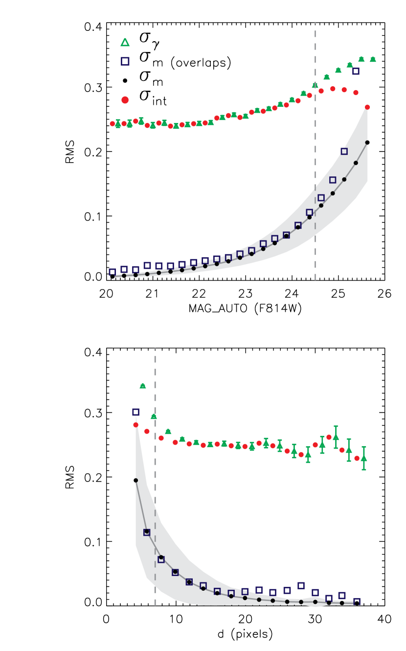
Figure 17: The observed scatter in the shear as a function of $F814W$ magnitude and size. The scatter is a combination of intrinsic shape noise, $\sigma_{int}$, and a shape measurement error, $\sigma_{meas}$. The shape measurement error is determined by a theoretical model and tested using galaxies from overlapping regions. Shaded regions indicate the RMS width of the measurement error distribution. The intrinsic shape noise appears to increase slightly as a function of magnitude but is independent of size. At faint magnitudes and small galaxy sizes, the shear scatter increases rapidly due to large measurement errors. The dashed vertical line indicates the size and magnitude cut that we apply in order to construct Figure 18.

Second, we derive an empirical estimation of the shape measurement error, $\sigma_{meas}$, using a sample of $27000$ galaxies that belong to overlapping regions of adjacent pointings. Each of these galaxies provide us with two independent shape measurements. Using these overlaps, we find that the shape measurement error is a function of both size and magnitude and increases beyond $\sigma_{meas}=0.1$ for $\textsc{mag\_auto}>24.5$ and $d<7$. Third, we compare this empirical determination of $\sigma_{meas}$ to the theoretical one derived in $\S$ 5.5. We find that the theoretical model of $\S$ 5.5 does remarkably well in predicting $\sigma_{meas}$ as a function of size and magnitude. Thus confident in the validity of this model, we adopt it for subsequent derivations. Finally, using equation 22 and the shear measurement error $\sigma_{meas}$, we extract the intrinsic shape noise of our galaxy sample as a function of size, magnitude and redshift. The results are shown in Figures 17 and 18.

As can be seen in Figure 17, large measurement errors lead to an increase of $\sigma_{\tilde{\gamma}}$ at small sizes and faint magnitudes. The intrinsic shape noise however, appears to change little with either size of magnitude and remains constant at a value of $\sigma_{int}\sim 0.26$. The slight apparent increase of the intrinsic shape noise at fainter magnitudes is probably due to the simplified measurement error estimator that we are using (indeed, the overlaps indicate slightly higher errors). From this analysis, we can draw the following conclusions:

• The intrinsic shape noise varies little from $z=0$ to $z=3$. Deep space based weak lensing surveys will therefore confront equivalent intrinsic shape noise floors as their shallower counterparts.

• Measurement errors lead to an increase in the shape noise as a function of size and magnitude. A joint improvement in both imaging quality as well as shape measurement methodology will lead to shape noises that are closer to the intrinsic floor of 0.26.

• We have yet to explore if the intrinsic shape noise varies as a function of galaxy type. If so, shear measurements could be improved by incorporating a galaxy-type discriminant into the weighting scheme. This will be the focus of a future paper.

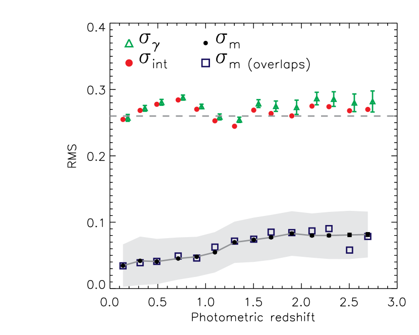
Figure 18: Intrinsic shape noise as a function of photometric redshift. Galaxies have first been selected to have measurement errors less than 0.1 ($d>7$ and $\textsc{mag\_auto}<24.5$) so that the scatter in the observed shear closely matches the intrinsic shape noise. A linear fit to the shape noise as a function of redshift reveals a flat distribution with a mean of $\sigma_{int}=0.26$.

8 Conclusion

We have carefully constructed a weak lensing catalog from 575 ACS/HST tiles, the largest space-based survey to date. We have established the quality of this catalog and analyzed the COSMOS redshift distribution, showing broad agreement with other photometric redshift surveys out to $z\sim 1$. The photometric redshifts are currently limited by the lack of deep $K$-band data but will rapidly improve as this data soon becomes available. Shapes have been measured for over $3.9\times 10^{5}$ galaxies and corrected for distortions induced by PSF and CTE effects. Simulations have been used in order to calibrate our shear measurement method and a STEP-like analysis has been performed, demonstrating our ability accurately measure shear with negligible additive and multiplicative bias. The effective number density of the COSMOS weak lensing catalog is $66$ galaxies per arcmin^-2 ($48$ when we consider only those with accurate photometric redshifts). A large fraction of these galaxies are at $z>1$ making COSMOS a powerful probe of the dark matter distribution and its evolution from $z=1$ to the present day. The COSMOS survey is also of foremost importance for the preparation and design of future wide field space-based lensing missions. Regarding the design of such missions, our main conclusions from working with the COSMOS data are the following:

1. Understanding and correcting for the time varying PSF and calibrating CTE effects were two of the most difficult challenges encountered with the COSMOS data. Reducing these two systematic effects should be a key specification in the design of next-generation telescopes and instruments.

2. Because 1) small galaxies are not as readily detected from the ground and 2) because larger areas are masked out in the ground-based data than in the ACS imaging, we lose 27% of our source sample when we select only those with accurate photometric redshifts.

3. The effective number density of galaxies is a very sensitive function of survey depth and resolution. The capability to resolve and accurately measure the shapes of very small, faint galaxies will be key in obtaining number densities of over 66 galaxies arcmin^-2.

4. Finally, we have derived the intrinsic shape noise of the galaxy sample and demonstrated that it remains fairly constant as a function of size, magnitude and redshift. Weak lensing measurements with deep space-based imaging are therefore on par with more shallow imaging in terms of the intrinsic shape noise floors that they must overcome.

The COSMOS weak lensing data described in this paper has already been used to measure cosmological parameters and to demonstrate the feasiblity of the “tomography” technique (Massey et al., 2007). Striking weak lensing mass maps of the COSMOS field have been made that reveal tantalizing evidence of a complex interplay between the baryon and the dark matter distribution (Massey et al., 2007a). Yet more lensing analyses are underway including a galaxy-galaxy lensing and a group-galaxy lensing study that will undoubtedly lead to a better understanding of the relationship between baryonic and dark matter structures and of its evolution over cosmic time.

References

- Bacon et al. (2006) Bacon, D. J., Goldberg, D. M., Rowe, B. T. P., & Taylor, A. N. 2006, MNRAS, 365, 414
- Bacon et al. (2001) Bacon, D. J., Refregier, A., Clowe, D., & Ellis, R. S. 2001, MNRAS, 325, 1065
- Bacon et al. (2005) Bacon, D. J. et al. 2005, MNRAS, 363, 723
- Bardeau et al. (2005) Bardeau, S., Kneib, J.-P., Czoske, O., Soucail, G., Smail, I., Ebeling, H., & Smith, G. P. 2005, A&A, 434, 433
- Bartelmann & Schneider (2001) Bartelmann, M. & Schneider, P. 2001, Phys. Rep., 340, 291
- Baugh & Efstathiou (1993) Baugh, C. M. & Efstathiou, G. 1993, MNRAS, 265, 145
- Bernstein & Jain (2004) Bernstein, G. & Jain, B. 2004, ApJ, 600, 17
- Bernstein & Jarvis (2002) Bernstein, G. M. & Jarvis, M. 2002, AJ, 123, 583
- Bertin & Arnouts (1996) Bertin, E. & Arnouts, S. 1996, A&AS, 117, 393
- Capak et al. (2004) Capak, P. et al. 2004, AJ, 127, 180
- Capak et al. (2007) Capak, P. L. et al. 2007, ApJS,
- Casertano et al. (2000) Casertano, S. et al. 2000, AJ, 120, 2747
- Coe et al. (2006) Coe, D., Benítez, N., Sánchez, S. F., Jee, M., Bouwens, R., & Ford, H. 2006, AJ, 132, 926
- Erben et al. (2001) Erben, T., Van Waerbeke, L., Bertin, E., Mellier, Y., & Schneider, P. 2001, A&A, 366, 717
- Ford et al. (2003) Ford, H. C. et al. 2003, in Future EUV/UV and Visible Space Astrophysics Missions and Instrumentation. Edited by J. Chris Blades, Oswald H. W. Siegmund. Proceedings of the SPIE, Volume 4854, pp. 81-94 (2003)., 81–94
- Goldberg & Bacon (2005) Goldberg, D. M. & Bacon, D. J. 2005, ApJ, 619, 741
- Goldberg & Leonard (2006) Goldberg, D. M. & Leonard, A. 2006, ArXiv Astrophysics e-prints
- Hetterscheidt et al. (2006) Hetterscheidt, M., Simon, P., Schirmer, M., Hildebrandt, H., Schrabback, T., Erben, T., & Schneider, P. 2006, ArXiv Astrophysics e-prints
- Heymans & Heavens (2003) Heymans, C. & Heavens, A. 2003, MNRAS, 339, 711
- Heymans et al. (2006) Heymans, C. et al. 2006, MNRAS, 368, 1323
- Heymans et al. (2005) Heymans, C. et al. 2005, MNRAS, 361, 160
- Highet al. (2007) High, F. W. 2007, in preparation
- Hoekstra et al. (2006) Hoekstra, H. et al. 2006, ApJ, 647, 116
- Hoekstra et al. (2004) Hoekstra, H., Yee, H. K. C., & Gladders, M. D. 2004, ApJ, 606, 67
- Ilbert et al. (2006) Ilbert, O. et al. 2006, ArXiv Astrophysics e-prints
- Impey et al. (1996) Impey, C. D., Sprayberry, D., Irwin, M. J., & Bothun, G. D. 1996, ApJS, 105, 209
- Jain & Taylor (2003) Jain, B. & Taylor, A. 2003, Physical Review Letters, 91, 141302
- Jarvis et al. (2006) Jarvis, M., Jain, B., Bernstein, G., & Dolney, D. 2006, ApJ, 644, 71
- Jee et al. (2005) Jee, M. J., White, R. L., Benítez, N., Ford, H. C., Blakeslee, J. P., Rosati, P., Demarco, R., & Illingworth, G. D. 2005, ApJ, 618, 46
- Kaiser et al. (1995) Kaiser, N., Squires, G., & Broadhurst, T. 1995, ApJ, 449, 460
- King (2005) King, L. J. 2005, A&A, 441, 47
- Kleinheinrich et al. (2005) Kleinheinrich, M. et al. 2005, A&A, 439, 513
- Kneib et al. (2003) Kneib, J.-P., Hudelot, P., Ellis, R. S., Treu, T., Smith, G. P., Marshall, P., Czoske, O., Smail, I., & Natarajan, P. 2003, ApJ, 598, 804
- Koekemoer (2007) Koekemoer, A. M. 2007, ApJS
- Koekemoer et al. (2002) Koekemoer, A. M., Fruchter, A. S., Hook, R. N., & Hack, W. 2002, in The 2002 HST Calibration Workshop : Hubble after the Installation of the ACS and the NICMOS Cooling System, Proceedings of a Workshop held at the Space Telescope Science Institute, Baltimore, Maryland, October 17 and 18, 2002. Edited by Santiago Arribas, Anton Koekemoer, and Brad Whitmore. Baltimore, MD: Space Telescope Science Institute, 2002., p.337, ed. S. Arribas, A. Koekemoer, & B. Whitmore, 337–+
- Krist (2005) Krist, J. 2005, Instrument Science Rep. ACS 2003-06 (Baltimore: STScI)
- Lilly et al. (2007) Lilly, S. J. et al. 2007, ApJS, 999, 999
- Lombardi et al. (2005) Lombardi, M. et al. 2005, ApJ, 623, 42
- Lupton et al. (2001) Lupton, R., Gunn, J. E., Ivezić, Z., Knapp, G. R., & Kent, S. 2001, in ASP Conf. Ser. 238: Astronomical Data Analysis Software and Systems X, ed. F. R. Harnden, Jr., F. A. Primini, & H. E. Payne, 269–+
- Mandelbaum et al. (2005) Mandelbaum, R., Seljak, U., Kauffmann, G., Hirata, C. M., & Brinkmann, J. 2005, ArXiv Astrophysics e-prints
- Massey et al. (2002) Massey, R., Bacon, D., Refregier, A., & Ellis, R. 2002, in ASP Conf. Ser. 283: A New Era in Cosmology, ed. N. Metcalfe & T. Shanks, 193–+
- Massey et al. (2006) Massey, R. et al. 2006, ArXiv Astrophysics e-prints
- Massey et al. (2004a) Massey, R., Refregier, A., Conselice, C. J., David, J., & Bacon, J. 2004a, MNRAS, 348, 214
- Massey et al. (2004b) —. 2004b, MNRAS, 348, 214
- Massey et al. (2007) Massey, R. et al. 2007, ApJS,
- Massey et al. (2007a) Massey, R., Rhodes, J., Ellis, R., Scoville, N., Leauthaud, A., Finoguenov, A., Capak, P., Bacon, D., Aussel, H., Kneib, J.-P., Koekemoer, A., McCracken, H., Mobasher, B., Pires, S., Refregier, A., Sasaki, S., Starck, J.-L., Taniguchi, Y., Taylor, A., & Taylor, J. 2007a, Nature, 445
- Mobasher et al. (2007) Mobasher, B. et al. 2007, ApJS
- Natarajan et al. (1998) Natarajan, P., Kneib, J.-P., Smail, I., & Ellis, R. S. 1998, ApJ, 499, 600
- Okura et al. (2006) Okura, Y., Umetsu, K., & Futamase, T. 2006, ArXiv Astrophysics e-prints
- Peterson et al. (1979) Peterson, B. et al. 1979, ApJ
- Refregier et al. (2002) Refregier, A., Rhodes, J., & Groth, E. J. 2002, ApJ, 572, L131
- Réfrégier et al. (2006) Réfrégier, A. et al. 2006, in High-Power Laser Ablation VI. Edited by Phipps, Claude R.. Proceedings of the SPIE, Volume 6265, pp. (2006).
- Rhodes et al. (2004) Rhodes, J., Refregier, A., Collins, N. R., Gardner, J. P., Groth, E. J., & Hill, R. S. 2004, ApJ, 605, 29
- Rhodes et al. (2000) Rhodes, J., Refregier, A., & Groth, E. J. 2000, ApJ, 536, 79
- Rhodes et al. (2001) —. 2001, ApJ, 552, L85
- Rhodes et al. (2007) Rhodes, J. D. et al. 2007, ApJS,
- Rix et al. (2004) Rix, H.-W. et al. 2004, ApJS, 152, 163
- Robin et al. (2007) Robin, A. et al. 2007, ApJS
- Robin et al. (2003) Robin, A. C., Reylé, C., Derrière, S., & Picaud, S. 2003, A&A, 409, 523
- Schrabback et al. (2006) Schrabback, T. et al. 2006, ArXiv Astrophysics e-prints
- Scoville et al. (2007) Scoville, N. Z. et al. 2007, ApJS
- Semboloni et al. (2006) Semboloni, E. et al. 2006, A&A, 452, 51
- Sheldon et al. (2004) Sheldon, E. S. et al. 2004, AJ, 127, 2544
- Taniguchi et al. (2007) Taniguchi, Y. et al. 2007, ApJS, 999-999
- Tyson et al. (1990) Tyson, J. A., Wenk, R. A., & Valdes, F. 1990, ApJ, 349, L1
- Williams et al. (1998) Williams, R. et al. 1998, Bulletin of the American Astronomical Society, 30, 1366
- Williams et al. (1996) Williams, R. E. et al. 1996, AJ, 112, 1335
- Wolf et al. (2004) Wolf, C. et al. 2004, A&A, 421, 913