The Halo Mass Function: High–Redshift Evolution and Universality

Abstract

We study the formation of dark matter halos in the concordance $\Lambda$CDM model over a wide range of redshifts, from $z=20$ to the present. Our primary focus is the halo mass function, a key probe of cosmology. By performing a large suite of nested-box $N$-body simulations with careful convergence and error controls (60 simulations with box sizes from 4 to 256$\,h^{-1}$Mpc), we determine the mass function and its evolution with excellent statistical and systematic errors, reaching a few percent over most of the considered redshift and mass range. Across the studied redshifts, the halo mass is probed over 6 orders of magnitude ($10^{7}$ – $10^{13.5}\,h^{-1}M_{\odot}$). Historically, there has been considerable variation in the high redshift mass function as obtained by different groups. We have made a concerted effort to identify and correct possible systematic errors in computing the mass function at high–redshift and to explain the discrepancies between some of the previous results. We discuss convergence criteria for the required force resolution, simulation box size, halo mass range, initial and final redshifts, and time stepping. Because of conservative cuts on the mass range probed by individual boxes, our results are relatively insensitive to simulation volume, the remaining sensitivity being consistent with extended Press-Schechter theory. Previously obtained mass function fits near $z=0$, when scaled by linear theory, are in good agreement with our results at all redshifts, although a mild redshift dependence consistent with that found by Reed et al. may exist at low redshifts. Overall, our results are consistent with a “universal” form for the mass function at high redshifts.

                                                                                                                                     LA-UR-06-0847

1 Introduction

A broad suite of astrophysical and cosmological observations provides compelling evidence for the existence of dark matter. Although its ultimate nature is unknown, the large-scale dynamics of dark matter is essentially that of a self-gravitating collisionless fluid. In an expanding universe, gravitational instability leads to the formation and growth of structure in the dark matter distribution. The existence of localized, highly overdense dark matter clumps, or halos, is a key prediction of cosmological nonlinear gravitational collapse. The distribution of dark matter halo masses is termed the halo mass function and constitutes one of the most important probes of cosmology. At low redshifts, $z\leq 2$, the mass function at the high-mass end (cluster scales) is very sensitive to variations in cosmological parameters, such as the matter content of the Universe $\Omega_{\rm m}$, the dark energy content along with its equation-of-state parameter, $w$ (Holder et al., 2001), and the normalization of the primordial fluctuation power spectrum, $\sigma_{8}$. At higher redshifts, the halo mass function is important in probing quasar abundance and formation sites Haiman & Loeb (2001), as well as the reionization history of the Universe Furlanetto et al. (2006).

Many recently suggested reionization scenarios are based on the assumption that the mass function is given reliably by modified Press-Schechter type fits (Press & Schechter 1974, hereafter PS; Bond et al. 1991). However, the theoretical basis of this approach is at best heuristic and careful numerical studies are required in order to obtain accurate results. Two examples serve to illustrate this statement. Reed et al. (2003) report a discrepancy with the Sheth-Tormen fit (Sheth & Tormen 1999, hereafter ST) of $\sim$50% at a redshift of $z=15$ (we explain the different fitting formulae and their origin in §2). Heitmann et al. (2006a) show that the Press-Schechter form can be severely incorrect at high redshifts: at $z\geq 10$, the predicted mass function sinks below the numerical results by an order of magnitude at the upper end of the relevant mass scale. Consequently, incorrect, or at best imprecise, predictions for the reionization history can result from the failure of fitting formulae.

Since halo formation is a complicated nonlinear gravitational process, the current theoretical understanding of the mass, spatial distribution, and inner profiles of halos remains at a relatively crude level. Numerical simulations are therefore crucial as drivers of theoretical progress, having been instrumental in obtaining important results such as the Navarro-Frenk-White (NFW) profile Navarro et al. (1997) for dark matter halos and an (approximate) universal form for the mass function (Jenkins et al.  2001, hereafter Jenkins). In order to better understand the evolution of the mass function at high redshifts, a number of numerical studies have been carried out. High–redshift simulations, however, suffer from their own set of systematic issues, and simulation results can be at considerable variance with each other, differing on occasion by as much as an order of magnitude!

Motivated by all of these reasons we have carried out a numerical investigation of the evolution of the mass function with the aim of attaining good control over both statistical and, more importantly, possible systematic errors in $N$-body simulations. Our first results have been reported in condensed form in Heitmann et al. (2006a). Here we provide a more detailed and complete exposition of our work, including several new results.

We first pay attention to simulation criteria for obtaining accurate mass functions with the aim of reducing systematic effects. Our two most significant points are that simulations must be started early enough to obtain accurate results and that the box sizes must be large enough to suppress finite-volume artifacts. As in most recent work following that of Jenkins, we define halo masses using a friends-of-friends (FOF) halo finder with linking length $b=0.2$. This choice introduces systematic issues of its own (e.g., connection to spherical overdensity mass as a function of redshift), which we touch on as relevant below. As it is not quantitatively significant in the context of this paper, we leave a detailed discussion to later work (Z. Lukić et al., in preparation; see also Reed et al. 2007).

The more detailed results in this paper enable us to study the mass function at statistical and systematic accuracies reaching a few percent over most of our redshift range, a substantial improvement over most previous work. At this level we find discrepancies with the “universal” fit of Jenkins at low redshifts ($z<5$), but it must be kept in mind that the universality of the original fit was only meant to be at the $\pm 20\%$ level. Recently, Reed et al. (2007) have found violation of universality at high redshifts (up to $z=30$). To fit the mass function they have incorporated an additional free parameter, the effective spectral index $n_{\rm eff}$, with the aim of understanding and taking into account the extra redshift dependence missing from conventional mass–function–fitting formulae. Our simulation results are consistent with the trends found by Reed et al. (2007) at low redshifts ($z\leq 5$), but at higher redshifts we do not observe a statistically significant violation of the universal form of the mass function.

Results from some previous simulations have reported good agreement with the Press-Schechter mass function at high redshifts. Since the Press-Schechter fit has been found significantly discrepant with low–redshift results ($z<5$), this would imply a strong disagreement with extending the well-validated low–redshift notion of (approximate) mass function universality to high $z$. Our conclusion is that the simulations on which these findings were based violated one or more of the criteria to be discussed below.

As simulations are perforce restricted to finite volumes, the obtained mass function clearly cannot represent that of an infinite box. Not only is sampling a key issue, but also the fact that simulations with periodic boundary conditions have no fluctuations on scales larger than the box size. To minimize and test for these effects we were conservative in our choices of box size and the mass range probed in each individual box. We also used nested-volume simulations to directly test for finite-volume effects. Because we used multiple boxes and averaged mass function results over the box ensemble, extended Press-Schechter theory can be used to correct for residual finite volume–effects (Mo & White 1996; Barkana & Loeb 2004); this approach is different from the individual box corrections applied by Reed et al. (2007). Details are given in §5.3.

The paper is organized as follows. In §2 we give a brief overview of the mass function and popular fitting formulae, discussing as well previous numerical work on the halo mass function at high redshifts. In §3 we give a short description of the $N$-body code MC² (Mesh-based Cosmology Code) and a summary of the performed simulations. In §4 we derive and discuss some simple criteria for the starting redshift and consider systematic errors related to the numerical evolution such as mass and force resolution and time stepping. These considerations in turn specify the input parameters for the simulations in order to span the desired mass and redshift range for our investigation. In §5 we present results for the mass function at different redshifts as well as the halo growth function. Here we also discuss the importance of post-processing corrections such as FOF particle sampling compensation and finite-volume effects. We discuss our results and conclude in §6.

2 Definitions and Previous Work

The mass function describes the number density of halos of a given mass. In order to determine the mass function in simulations one has to first identify the halos and then define their mass. No precise theoretical basis exists for these operations. Nevertheless, depending on the situation at hand, the observational and numerical communities have adopted a few “standard” ways of defining halos and their associated masses. For a recent review of these issues with regard to observations, see, e.g.,  Voit (2005), but for a more theoretically oriented review, see, e.g., White (2001).

2.1 Halo Mass

There are basically two ways to find halos in a simulation. One, the overdensity method, is based on identifying overdense regions above a certain threshold. The threshold can be set with respect to the critical density $\rho_{\rm c}=3H^{2}/8\pi G$ (or the background density $\rho_{\rm b}=\Omega_{\rm m}\rho_{\rm c}$, where $\Omega_{\rm m}$ is the matter density of the Universe including dark matter and baryons). The mass $M_{\Delta}$ of a halo identified this way is defined as the mass enclosed in a sphere of radius $r_{\Delta}$ whose mean density is $\Delta\rho_{\rm c}$. Common values for $\Delta$ range from 100 to 500 (or even higher). As explained in Voit (2005), cluster observers prefer higher values for $\Delta$. Properties of clusters are easier to observe in higher density regions and these regions are more relaxed than the outer parts which are subject to the effects of inflow and incomplete mixing. The disadvantage of defining a halo in this manner is that sphericity of halos is implied, an assumption which may be easily violated, e.g., in the case of halos that formed in a recent merger event or halos at high redshifts. At higher redshifts, the nonlinear mass scale $M_{*}$ decreases rapidly, and the ratio of the considered halo mass $M_{\rm halo}$ to $M_{*}$ can become large. This translates into producing large-scale structures roughly analogous to supercluster structures today. While these structures are gravitationally bound, they are often not virialized, nor spherical. Even the much smaller structures (which are considered in this paper) are not virialized at high redshifts, and therefore, assumptions about sphericity are most likely violated. Hence the spherical overdensity method does not suggest itself as an obvious way to identify halos at high redshift.

The other method, the FOF algorithm, is based on finding neighbors of particles and neighbors of neighbors as defined by a given separation distance (see, e.g., Einasto et al. 1984; Davis et al. 1985). The FOF algorithm leads to halos with arbitrary shapes since no prior symmetry assumptions have been made. The halo mass is defined simply as the sum of particles which are members of the halo. While this definition is easy to apply to simulations, the connection to observations is difficult to establish directly. (For an investigation of connections between different definitions of halos masses and approximate conversions between them, see White 2001).

It is important to keep in mind that the definition of a halo is essentially the adoption of some sort of convention for the halo boundary. In reality, a sharp distinction between the particles in a halo and particles in the simulation “field” does not exist. Jenkins showed that the choice of a FOF finder with a linking length $b=0.2$ to define halo masses provides the best fit for a universal form of the mass function. This choice has since been adopted by many numerical practitioners as a standard convention. A useful discussion of the various halo definitions can be found in White (2002).

In this paper we use the FOF algorithm to identify halos and their masses. It was recently pointed out by Warren et al. (2006, hereafter Warren) that FOF masses suffer from a systematic problem when halos are sampled by relatively small numbers of particles. Although halos can be robustly identified with as few as 20 particles, if a given halo has too few particles, its FOF mass turns out to be systematically too high. We describe how we compensate for this effect in §5.2. In the current paper, all results for the mass function are displayed at a fixed FOF linking length of $b=0.2$, using the Warren correction.

2.2 Defining the Mass Function

The exact definition of the mass function, e.g., integrated versus differential form or count versus number density, varies widely in the literature. To characterize different fits, Jenkins introduced the scaled differential mass function $f(\sigma,z)$ as a fraction of the total mass per $\ln\sigma^{-1}$ that belongs to halos:

$$f(\sigma,z)\equiv\frac{d\rho/\rho_{b}}{d\ln\sigma^{-1}}=\frac{M}{\rho_{\rm b}(z)}\frac{dn(M,z)}{d\ln[\sigma^{-1}(M,z)]}.$$ (1)

Here $n(M,z)$ is the number density of halos with mass $M$, $\rho_{\rm b}(z)$ is the background density at redshift $z$, and $\sigma(M,z)$ is the variance of the linear density field. As pointed out by Jenkins, this definition of the mass function has the advantage that to a good accuracy it does not explicitly depend on redshift, power spectrum, or cosmology; all of these are encapsulated in $\sigma(M,z)$. For the most part, we will display the mass function

$$F(M,z)\equiv{dn\over d\log M}$$ (2)

as a function of $\log M$ itself. [In §5 we include results for $f(\sigma,z)$.]

To compute $\sigma(M,z)$, the power spectrum $P(k)$ is smoothed with a spherical top-hat filter function of radius $R$, which on average encloses a mass $M$ ($R=[3M/4\pi\rho_{\rm b}(z)]^{1/3}$):

$$\sigma^{2}(M,z)=\frac{d^{2}(z)}{2\pi^{2}}\int^{\infty}_{0}k^{2}P(k)W^{2}(k,M)dk,$$ (3)

where $W(k,M)$ is the top-hat filter:

$$W(r) = \left\{\begin{array}[]{rl}\frac{3}{4\pi R^{3}},&r<R\\ 0,&r>R\end{array}\right.$$ (6)

$$W(k) = \frac{3}{(kR)^{3}}\left[\sin(kR)-kR\cos(kR)\right].$$ (7)

The redshift dependence enters only through the growth factor $d(z)$, normalized so that $d(0)=1$:

$$\sigma(M,z)=\sigma(M,0)d(z).$$ (8)

In the approximation of negligible difference in the CDM and baryon peculiar velocities, the growth function in a $\Lambda$CDM universe is given by (Peebles 1980)

$$d(a)=\frac{D^{+}(a)}{D^{+}(a=1)},$$ (9)

where we consider $d$ as a function of the cosmological scale factor $a=1/(1+z)$, and

$$D^{+}(a)=\frac{5\Omega_{\rm m}}{2}\,\frac{H(a)}{H_{0}}\int_{0}^{a}\frac{da^{\prime}}{[a^{\prime}H(a^{\prime})/H_{0}]^{3}}$$ (10)

with $H(a)/H_{0}=\left[\Omega_{\rm m}/a^{3}+(1-\Omega_{\rm m})\right]^{1/2}$. In particular, for $z\gg 1$, when matter dominates the cosmological constant, $D^{+}(a)\simeq a$.

Even in linear theory, equation (10) is only an approximation because baryons began their gravitational collapse with velocities different from those of CDM particles. Until recombination at $z\sim 1100$, well into the matter era with non-negligible growth of CDM inhomogeneities, the baryons were held against collapse by the pressure of the CMB photons (see, e.g. Hu & Sugiyama (1996)). While thereafter the relative baryon-CDM velocity decayed as $1/a$, the residual velocity difference was sufficient to affect the growth function $d(z)$ at $z=50$ by more than $1\%$ and at $z=10$ by about $0.2\%$ (Yoshida et al. 2003; Naoz & Barkana 2007).

2.3 Fitting Functions

Over the last three decades several different fitting forms for the mass function have been suggested. The mass function is not only a sensitive measure of cosmological parameters by itself but also a key ingredient in analytic and semianalytic modeling of the dark matter distribution, as well as of several aspects of the formation, evolution, and distribution of galaxies. Therefore, if a reliable and accurate fit for the mass function applicable to a wide range of cosmologies and redshifts were to exist, it would be of obvious utility. In this section we briefly review the common fitting functions and compare them at different redshifts.

The first analytic model for the mass function was developed by PS. Their theory accounts for a spherical overdense region in an otherwise smooth background density field, which then evolves as a Friedmann universe with a positive curvature. Initially, the overdensity expands, but at a slower rate than the background universe (thus enhancing the density contrast), until it reaches the ‘turnaround’ density, after which collapse begins. Although from a purely gravitational standpoint this collapse ends with a singularity, it is assumed that in reality – due to the spherical symmetry not being exact – the overdense region will virialize. For an Einstein-de Sitter universe, the density of such an overdense region at the virialization redshift is $z\approx 180\rho_{\rm c}(z)$. At this point, the density contrast from the linear theory of perturbation growth [$\delta(\vec{x},z)=d(z)\delta(\vec{x},0)$] would be $\delta_{\rm c}(z)\approx 1.686$ in an Einstein-de Sitter cosmology. For $\Omega_{\rm m}<1$, the value of the threshold parameter $\delta_{\rm c}$ can vary (see Lacey & Cole 1993), but the dependence on cosmology has little quantitative significance (see, e.g., Jenkins). Thus, throughout this paper we adopt $\delta_{\rm c}=1.686$.

Table 1: Mass Function Fits for $f(\sigma)$

Reference	Fitting Function $f(\sigma)$	Mass Range	Redshift range
ST, Sheth & Tormen (2001)	$0.3222\sqrt{\frac{2a}{\pi}}\frac{\delta_{\rm c}}{\sigma}\exp\left[-\frac{a\delta^{2}_{\rm c}}{2\sigma^{2}}\right]\left[1+\left(\frac{\sigma^{2}}{a\delta^{2}_{\rm c}}\right)^{p}\right]$	unspecified	unspecified
Jenkins	$0.315\exp\left[-|\ln\sigma^{-1}+0.61|^{3.8}\right]$	$-1.2\leq\ln\sigma^{-1}\leq 1.05$	$z=0-5$
Reed et al. (2003)	$f_{\rm ST}(\sigma)\,\exp\left\{-0.7/\left[\sigma(\cosh(2\sigma))^{5}\right]\right\}$	$-1.7\leq\ln\sigma^{-1}\leq 0.9$	$z=0-15$
Warren	$0.7234\left(\sigma^{-1.625}+0.2538\right)\exp\left[-\frac{1.1982}{\sigma^{2}}\right]$	$(10^{10}-10^{15})h^{-1}M_{\odot}$	$z=0$
Reed et al. (2007)	$A\sqrt{\frac{2a}{\pi}}\left[1+\left(\frac{\sigma^{2}}{a\delta_{c}^{2}}\right)^{p}+0.6G_{1}(\sigma)+0.4G_{2}(\sigma)\right]$	$-0.5\leq\ln\sigma^{-1}\leq 1.2$	$z=0-30$
	$\times\frac{\delta_{c}}{\sigma}\exp\left[-\frac{ca\delta_{c}^{2}}{2\sigma^{2}}-\frac{0.03}{(n_{\rm eff}+3)^{2}}\left(\frac{\delta_{c}}{\sigma}\right)^{0.6}\right]$

Following the above reasoning and with the assumption that the initial density perturbations are described by a homogeneous and isotropic Gaussian random field, the PS mass function is specified by

$$f_{\rm PS}(\sigma)=\sqrt{\frac{2}{\pi}}\frac{\delta_{\rm c}}{\sigma}\exp\left(-\frac{\delta^{2}_{\rm c}}{2\sigma^{2}}\right).$$ (11)

The PS approach assumes that all mass is inside halos, as enforced by the constraint

$$\int^{+\infty}_{-\infty}f_{\rm PS}(\sigma)\,d\ln\sigma^{-1}=1.$$ (12)

While as a first rough approximation the PS mass function agrees with simulations at $z=0$ reasonably well, it overpredicts the number of low–mass halos and underpredicts the number of massive halos at the current epoch. Furthermore, it is significantly in error at high redshifts (see, e.g., Springel et al. 2005; Heitmann et al. 2006a; §5.4).

After PS, several suggestions were made in order to improve the mass function fit. These suggestions were based on more refined dynamical modeling, direct fitting to simulations, or a combination of the two.

Using empirical arguments ST proposed an improved mass function fit of the form:

$$f_{\rm ST}(\sigma)=0.3222\sqrt{\frac{2a}{\pi}}\frac{\delta_{\rm c}}{\sigma}\exp\left(-\frac{a\delta^{2}_{\rm c}}{2\sigma^{2}}\right)\left[1+\left(\frac{\sigma^{2}}{a\delta^{2}_{\rm c}}\right)^{p}\right],$$ (13)

with $a=0.707$ and $p=0.3$. (Sheth & Tormen 2002 suggest $a=0.75$ as an improved value.) Sheth et al. (2001) rederived this fit theoretically by extending the PS approach to an elliptical collapse model. In this model, the collapse of a region depends not only on its initial overdensity but also on the surrounding shear field. The dependence is chosen such that it recovers the Zel’dovich approximation Zel’dovich (1970) in the linear regime. A halo is considered virialized when the third axis collapses (see also Lee & Shandarin (1998) for an earlier, different approach to the same idea).

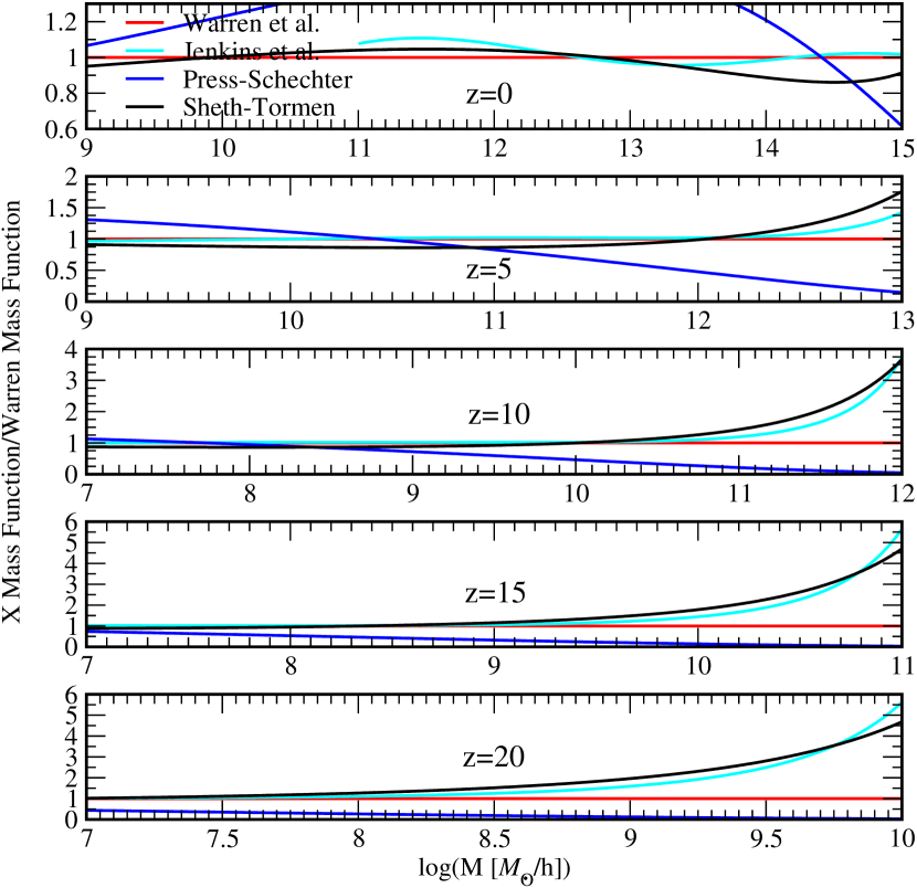
Figure 1: Ratio of the Jenkins, PS, and ST mass function fits with respect to the Warren fit for five different redshifts over a range of halo masses. Top to bottom: Redshifts $z=0$, 5, 10, 15, and 20. Note that the ranges of the axes are different in the different panels. We do not show the Jenkins fit below masses of 10${}^{11}h^{-1}M_{\odot}$ at $z=0$, since it is not valid for such low masses at that redshift.

Jenkins combined high resolution simulations for four different CDM cosmologies ($\tau$CDM, SCDM, $\Lambda$CDM, and OCDM) spanning a mass range of over 3 orders of magnitude ($\sim(10^{12}-10^{15})\,h^{-1}M_{\sun}$), and including several redshifts between $z=5$ and 0. Independent of the underlying cosmology, the following fit provided a good representation of their numerical results (within $\pm 20\%$):

$$f_{\rm Jenkins}(\sigma)=0.315\exp\left(-|\ln\sigma^{-1}+0.61|^{3.8}\right).$$ (14)

The above formula is very close to the Sheth-Tormen fit, leading to some improvement at the high-mass end. The disadvantage is that it cannot be simply extrapolated beyond the range of the fit, since it was tuned to a specific set of simulations.

By performing 16 nested-volume dark matter simulations, Warren was able to obtain significant halo statistics spanning a mass range of 5 orders of magnitude ($\sim(10^{10}-10^{15})\,h^{-1}M_{\sun}$). Because this represents by far the largest uniform set of simulations–based on multiple boxes with the same cosmology run with the same code–we use it as a reference standard throughout this paper. Using a functional form similar to ST, Warren determined the best mass function fit to be

$$f_{\rm Warren}(\sigma)=0.7234\left(\sigma^{-1.625}+0.2538\right)\exp\left(-\frac{1.1982}{\sigma^{2}}\right).$$ (15)

For a quantitative comparison of the different fits at different redshifts, we show the ratio of the PS, Jenkins, and ST fits with respect to the Warren fit in Figure 1. We do not show the Jenkins fit below $10^{11}\,h^{-1}M_{\odot}$ at $z=0$ since it diverges in this regime. The original ST fit, the Jenkins fit, and the Warren fit all give similar predictions. The discrepancy between PS and the other fits becomes more severe for higher masses at high redshifts. PS dramatically underpredicts halos in the high-mass range at high redshifts (assuming that the other fits lead to reasonable results in this regime). For low-mass halos the disagreement becomes less severe. For $z=0$ the Warren fit agrees, especially in the low-mass range below $10^{13}\,h^{-1}M_{\odot}$, to better than 5% with the ST fit. At the high-mass end the difference increases up to 20%. The Jenkins fit leads to similar results over the considered mass range. At higher redshifts and intermediate-mass ranges around $10^{9}\,h^{-1}M_{\odot}$, the Warren and ST fit disagree by roughly a factor of 2.

Several other groups have suggested modifications of the ST fit. In §5 we compare our results with two of them. Reed et al. (2003) suggest an empirical adjustment to the ST fit by multiplying it with an exponential function, leading to

$$f_{\rm Reed03}(\sigma)=f_{\rm ST}(\sigma)\,\exp\left\{-0.7/\left[\sigma(\cosh(2\sigma))^{5}\right]\right\},$$ (16)

valid over the range $-1.7\leq\ln\sigma^{-1}\leq 0.9$. This adjustment leads to a suppression of the ST fit at large $\sigma^{-1}$. In Reed et al. (2007) the adjustment to the ST fit is slightly modified again, leading to the following new fit:

$$f_{\rm Reed07}(\sigma) = A\sqrt{\frac{2a}{\pi}}\left[1+\left(\frac{\sigma^{2}}{a\delta_{c}^{2}}\right)^{p}+0.6G_{1}+0.4G_{2}\right]$$ (17)

$$\times\frac{\delta_{c}}{\sigma}\exp\left[-\frac{ca\delta_{c}^{2}}{2\sigma^{2}}-\frac{0.03}{(n_{\rm eff}+3)^{2}}\left(\frac{\delta_{c}}{\sigma}\right)^{0.6}\right],$$

$$G_{1} = \exp\left[-\frac{\ln(\sigma^{-1}-0.4)^{2}}{2(0.6)^{2}}\right],$$ (18)

$$G_{2} = \exp\left[-\frac{\ln(\sigma^{-1}-0.75)^{2}}{2(0.2)^{2}}\right],$$ (19)

with $c=1.08$, $ca=0.764$, and $A=0.3222$. The adjustment has very similar effects to that of Reed et al. (2003), as we show in §5. Reed et al. (2007) note that the (small) suppression of the mass function relative to ST as a function of redshift seen in simulations (see also Heitmann et al. 2006a) can be treated by adding an extra parameter, the power spectral slope at the scale of the halo radius, $n_{\rm eff}$ (formally defined by equation (44) below). We return to this issue when we discuss our numerical results in §5. We summarize the described, most commonly used fitting functions in Table 1.

Although fitting functions may be a useful way to approximately encapsulate results from simulations, meaningful comparisons to observations require overcoming many hurdles, e.g., an operational understanding of the definition of halo mass (see, e.g., White 2001), how it relates to various observations, and error control in $N$-body codes (see, e.g., O’Shea et al. 2005; Heitmann et al. 2005). In this paper, our focus is first on identifying possible systematic problems in the $N$-body simulations themselves and how they can be avoided and controlled.

2.4 Halo Growth Function

A useful way to study the statistical evolution of halo masses in simulations is to transform the mass function into the halo growth function, $n(M_{1},M_{2},z)\equiv\int_{M_{1}}^{M_{2}}F\,d\log M$ Heitmann et al. (2006a), which measures the mass-binned number density of halos as a function of redshift. The halo growth function, plotted versus redshift in Figure 2, shows at a glance how many halos in a particular mass bin and box volume are expected to exist at a certain redshift. This helps set the required mass and force resolution in a simulation which aims to capture halos at high redshifts. For a given simulation volume, the halo growth function directly predicts the formation time of the first halos in a given mass range.

In order to derive this quantity approximately, we first convert an accurate mass function fit (we use the Warren fit here) into a function of redshift $z$. It has been shown recently by us (Heitmann et al. 2006a) that mass function fits work reliably enough out to at least $z=20$, and can therefore be used to estimate the halo growth function. Figure 2 shows the evolution of eight different mass bins, covering the mass range investigated in this paper, as a function of redshift $z$. As expected from the paradigm of hierarchical structure formation in a $\Lambda$CDM cosmology, small halos form much earlier than larger ones. An interesting feature in the lower mass bins is that they have a maximum at different redshifts. The number of the smallest halos grows until a redshift of $~{}z=2$ and then declines when halos start merging and forming much more massive halos. This feature is reflected in a crossing of the mass functions at different redshifts for small halos.

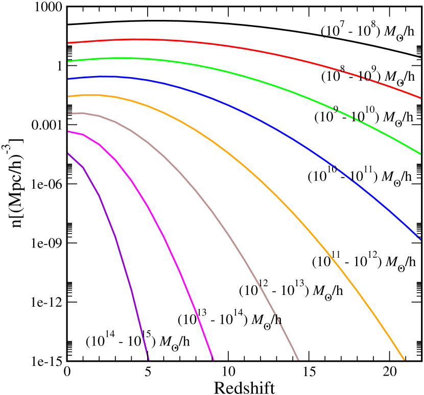
Figure 2: Halo growth function based on the Warren mass function fit for different mass bins. The curves for the lower mass bins have a maximum at $z>0$ which reflects a crossover of the mass functions at different redshifts.

2.5 Mass Function at High Redshift: Previous Work

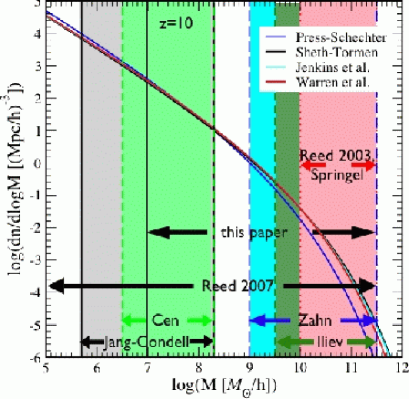
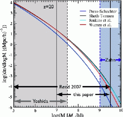
Figure 3: Summary of recent work on the mass function at high redshift. The mass function fits are shown at $z=10$ (top) and $z=20$ (bottom) for the cosmology used throughout this paper (the other groups used slightly different parameters). At $z=10$, Jang-Condell & Hernquist (2001) (gray shaded region) cover the very low mass range using a very small box, as do Cen et al. (2004) (green shaded region). The larger boxes of Reed et al. (2007) and Springel et al. (2005) (red shaded region) lead to results at higher halo masses. Note that in this regime the PS fit deviates substantially from the other fits, while at the very low mass end all fits tend to merge. Our suite of variable box sizes covers a mass range of 10⁷ to 10${}^{13.5}\,h^{-1}M_{\odot}$ between $z=0$ and 20, a much larger range than previously covered by any group with a uniform set of simulations. At $z=20$ Yoshida et al. (2003a, 2003b, 2003c, 2003d) cover the very low mass end of the mass function, while Zahn et al. (2007) investigate larger mass halos. Our simulations overlap with both of them at the edges. By combining a heterogeneous set of simulations, Reed et al. (2007) cover a wide range in mass and redshift. Figure quality reduced for the arXiv version of the paper.

Table 2: Summary of the Performed Runs

	Box Size	Resolution			Particle Mass	Smallest Halo
Mesh	($h^{-1}$Mpc)	($h^{-1}$kpc)	$z_{\rm in}$	$z_{\rm final}$	($h^{-1}M_{\odot}$)	($h^{-1}M_{\odot}$)	No. of Realizations
10243	256	250	100	0	$8.35\times 10^{10}$	$3.34\times 10^{12}$	5
10243	128	125	200	0	$1.04\times 10^{10}$	$4.18\times 10^{11}$	5
10243	64	62.5	200	0	$1.31\times 10^{9}$	$5.22\times 10^{10}$	5
10243	32	31.25	150	5	$1.63\times 10^{8}$	$6.52\times 10^{9}$	5
10243	16	15.63	200	5	$2.04\times 10^{7}$	$8.16\times 10^{8}$	5
10243	8	7.81	250	10	$2.55\times 10^{6}$	$1.02\times 10^{8}$	20
10243	4	3.91	500	10	$3.19\times 10^{5}$	$1.27\times 10^{7}$	15

Most of the effort to characterize, fit, and evaluate the mass function from simulations has been focused on or near the current cosmological epoch, $z\sim 0$. This is mainly for two reasons: (1) so far most observational constraints have been derived from low-redshift objects ($z<1$); (2) the accurate numerical evaluation of the mass function at high redshifts is a nontrivial task.

The increasing reach of telescopes on the ground and in space, such as the upcoming James Webb Space Telescope, allows us to study the Universe at higher and higher redshifts. Recent discoveries include 970 galaxies at redshifts between $z=1.5$ and $z=5$ from the VIMOS VLT Deep Survey Le Fevre et al. (2005), and the recent observation of a galaxy at $z=6.5$ Mobasher et al. (2005). The epoch of reionization (EOR) is of central importance to the formation of cosmic structure. Although our current observational knowledge of the EOR is rather limited, future 21 cm experiments have the potential for revolutionizing the field. Proposed low-frequency radio telescopes include LOFAR (Low Frequency Array) , the Mileura Wide Field Array (MWA) Bowman et al. (2006), and the next-generation SKA (Square Kilometer Array) . The observational progress is an important driver for high-redshift mass function studies.

Theoretical studies of the mass function at high redshifts are challenging due to the small masses of the halos at early times. In order to capture these small-mass halos, high mass and force resolution are both required. For the large simulation volumes typical in cosmological studies, this necessitates a very large number of particles, as well as very high force resolution. Such simulations are very costly, and only a very limited number can be performed, disallowing exploration of a wide range of possible simulation parameters. Alternatively, many smaller volume simulation boxes, each with moderate particle loading, can be employed. This leads automatically to high force and mass resolution in grid codes (such as particle-mesh [PM]) and also reduces the costs for achieving sufficient resolution for particle codes (such as tree codes) or hybrid codes (such as TreePM). The disadvantages of this strategy are the limited statistics in individual realizations (because fewer halos form in a smaller box) and the unreliability of simulations below an intermediate redshift at which the largest mode in the box is still (accurately) linear. In addition, results from small boxes may be biased, since they only focus on a small region and volume. Therefore, one must show that the simulations are free from finite-volume artifacts, e.g. missing tidal forces, and run a sufficient number of statistically independent simulations to reduce the sample variance. Both strategies, employing large volume or multiple small-volume simulations, have been followed in the past in order to obtain results at high redshifts. The different mass ranges investigated by different groups are shown in Figure 3. The fits are shown for redshifts $z=10$ and 20. In the Appendix we provide a very detailed discussion on previous findings as organized by simulation volume.

In summary, there is considerable variation in the high-redshift ($z>10$) mass function as found by different groups, independent of box size and simulation algorithm. Broadly speaking, the results fall into two classes: either consistent with linear theory scaling of a universal form (Jenkins, Reed, ST, or Warren) at low redshift (Reed et al. 2003, 2007; Springel et al. 2005; Heitmann et al. 2006a; Maio et al. 2006; Zahn et al. 2007) or more consistent with the PS fit (Jang-Condell & Hernquist 2001; Yoshida et al. 2003a, 2003b, 2003c; Cen et al. 2004; Iliev et al. 2006; Trac & Cen 2006).

Our aim here is to determine the evolution of the mass function accurately, at the few percent level, and at the same time characterize many of the numerical and physical factors that control the error in the mass function (details below). We follow up on our previous work Heitmann et al. (2006a) and analyze a large suite of $N$-body simulations with varying box sizes between 4 and $256\,h^{-1}$Mpc, including many realizations of the small boxes, to study the mass function at redshifts up to $z=20$ and to cover a large mass range between $10^{7}$ and $10^{13.5}\,h^{-1}M_{\odot}$. With respect to our previous work, the number of small-box realizations has been increased to improve the statistics at high redshifts. Our results categorically rule out the PS fit as being more accurate than any of the more modern forms at any redshift up to $z=20$, the discrepancy increasing with redshift.

3 The Code and the Simulations

All simulations in this paper are carried out with the parallel PM code MC². This code solves the Vlasov-Poisson equations for an expanding universe. It uses standard mass deposition and force interpolation methods allowing periodic or open boundary conditions with second-order (global) symplectic time stepping and fast fourier transform based Poisson solves. Particles are deposited on the grid using the cloud-in-cell method. The overall computational scheme has proven to be accurate and efficient: relatively large time steps are possible with exceptional energy conservation being achieved. MC² has been extensively tested against state-of-the-art cosmological simulation codes (Heitmann et al. 2005, 2007).

We use the following cosmology for all simulations:

$$\Omega_{\rm tot}=1.0,~{}~{}~{}\Omega_{\rm CDM}=0.253,~{}~{}~{}\Omega_{\rm baryon}=0.048,$$

$$\sigma_{8}=0.9,~{}~{}~{}H_{0}=70\ {\rm km\ s^{-1}\,Mpc^{-1}},~{}~{}~{}n=1,$$ (20)

in concordance with cosmic microwave background and large scale structure observations MacTavish et al. (2006) (the third-year Wilkinson Microwave Anisotropy Probe observations suggest a lower value of $\sigma_{8}$; Spergel et al. (2007)). The transfer functions are generated with CMBFAST Seljak & Zaldarriaga (1996). We summarize the different runs, including their force and mass resolution, in Table 2. As mentioned earlier, we identify halos with a standard FOF halo finder with a linking length of $b=0.2$. Despite several shortcomings of the FOF halo finder, e.g., the tendency to link up two halos which are close to each other (see, e.g., Gelb & Bertschinger 1994, Summers et al. 1995) or statistical biases (Warren), the FOF algorithm itself is well defined and very fast. As discussed in §2.1, we adopt the correction for sampling bias given by Warren when presenting our results.

4 Initial Conditions and Time Evolution

In a near-ideal simulation with very high mass and force resolution, the first halos would form very early. By $z=50$, a redshift commonly used to start cosmological simulations, a large number of small halos would already be present (see, e.g., Reed et al. [2005] for a discussion of the first generation of star-forming halos). In a more realistic situation, however, the initial conditions at $z=50$ have of course no halos, the particles having moved only the relatively small distance assigned by the initial Zel’dovich step. Only after the particles have traveled a sufficient distance and come close together can they interact locally to form the first halos. In the following we estimate the redshift when the Zel’dovich grid distortion equals the interparticle spacing, leading to the most conservative estimate for the redshift of possible first halo formation. From this estimate, we derive the necessary criterion for the starting redshift for a given box size and particle number.

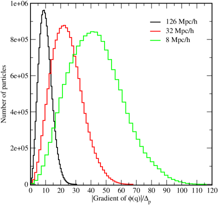
Figure 4: Probability distribution of $|\nabla{\bf\phi}|$ in units of the interparticle spacing $\Delta_{\rm p}$. All curves shown are drawn from $256^{3}$ particle simulations from an initial density grid of $256^{3}$ zones. The physical box sizes are $126\,h^{-1}$Mpc (black line), $32\,h^{-1}$Mpc (red line), and $8\,h^{-1}$Mpc (green line). As expected, $\langle|\nabla{\bf\phi}|\rangle$ increases with decreasing box size (which is equivalent to increasing force resolution). Therefore, $z_{\rm in}$ and $z_{\rm cross}$ are higher for the smaller boxes.

4.1 Initial Redshift

In order to capture halos at high redshifts, we have found that it is very important to start the simulation sufficiently early. We consider two criteria for setting the starting redshift: (1) ensuring the linearity of all the modes in the box used to sample the initial matter power spectrum, and (2) restricting the initial particle move to prevent interparticle crossing and to keep the particle grid distortion relatively small. The first criterion is commonly used to identify the starting redshift in simulations. However, as shown below, it fails to provide sufficient accuracy of the mass functions, accuracy which can be obtained when a second (much more restrictive) control is applied. Furthermore, it is important to allow a sufficient number of expansion factors between the starting redshift $z_{\rm in}$ and the highest redshift of physical significance. This is needed to make sure that artifacts from the Zel’dovich approximation are negligible and that the memory of the artificial particle distribution imposed at $z_{\rm in}$ (grid or glass) is lost by the time any halo physics is to be extracted from the simulation results.

Although not studied here, it is important to note that high-redshift starts do require the correct treatment of baryons as noted in §2.2. In addition, redshift starts that are too high can lead to force errors for a variety of reasons, e.g., interpolation systematics, round-off, and correlated errors in tree codes.

4.1.1 Initial Perturbation Amplitude

Table 3: Initial Redshift Estimates from the Linearity of $\Delta^{2}(k_{\rm Ny})$

Box Size	$k_{\rm Ny}$
($h^{-1}$Mpc)	($h$ Mpc-1)	$T(z=0,\,k_{\rm Ny})$	$z_{\rm in}$
126	6.3	0.0002	33
32	25	1.7$\cdot 10^{-5}$	45
16	50	4.8$\cdot 10^{-6}$	50
8	100	1.3$\cdot 10^{-6}$	55

The initial redshift in simulations is often determined from the requirement that all mode amplitudes in the box below the particle Nyquist wavenumber characterized by $k_{\rm Ny}/2$ with $k_{\rm Ny}=2\pi/\Delta_{\rm p}$, where $\Delta_{\rm p}$ is the mean interparticle spacing, be sufficiently linear. The smaller the box size chosen (keeping the number of particles fixed), the larger the largest $k$-value. Therefore, in order to ensure that the smallest initial mode in the box is well in the linear regime, the starting redshift must increase as the box size decreases. In the following we give an estimate based on this criterion for the initial redshift for different simulation boxes. We (conservatively) require the dimensionless power spectrum $\Delta^{2}=k^{3}P(k)/2\pi^{2}$ to be smaller than $0.01$ at the initial redshift. The initial power spectrum is given by

$$\Delta^{2}(k_{\rm Ny},z_{\rm in})=\frac{k^{3}P(k_{\rm Ny},z_{\rm in})}{2\pi^{2}}\sim\frac{B\ k^{n+3}T^{2}(k_{\rm Ny},z=0)}{2\pi^{2}(z_{\rm in}+1)^{2}},$$ (21)

where $B$ is the normalization of the primordial power spectrum (see, e.g., Bunn & White [1997] for a fitting function for $B$ including COBE results) and $T(k)$ is the transfer function. We assume the spectral index to be $n=1$, which is sufficient to obtain an estimate for the initial redshift. For a $\Lambda$CDM universe the normalization is roughly $B\sim 3.4\times 10^{6}(h^{-1}{\rm Mpc})^{4}$. Therefore, $z_{\rm in}$ is simply determined by

$$z_{\rm in}\simeq 4150\ k_{\rm Ny}^{2}T(z=0,k_{\rm Ny}).$$ (22)

We present some estimates for different box sizes in Table 3. For the smaller boxes ($<8~{}h^{-1}$Mpc), the estimates for the initial redshifts are at around $z_{\rm in}=50$.

It is clear that this criterion simply sets a minimal requirement for $z_{\rm in}$ and neglects the fact that the initial particle move should be small enough to maintain the dynamical accuracy of perturbation theory (linear or higher order) used to set the initial conditions. Also, this criterion certainly does not tell us that if, e.g., $z_{\rm in}=50$, then we may already trust the mass function at, say, $z=30$. An example of this is provided by the results of Reed et al. (2003), who find that their high-redshift results between $z=7$ and 15 have not converge if they start their simulations at $z_{\rm in}=69$. (A value of $z_{\rm in}=139$ was claimed to be sufficient in their case.)

We now consider another criterion – ostensibly similar in spirit – that particles should not move more than a certain fraction of the interparticle spacing in the initialization step. This second criterion demands much higher redshift starts.

4.1.2 First Crossing Time

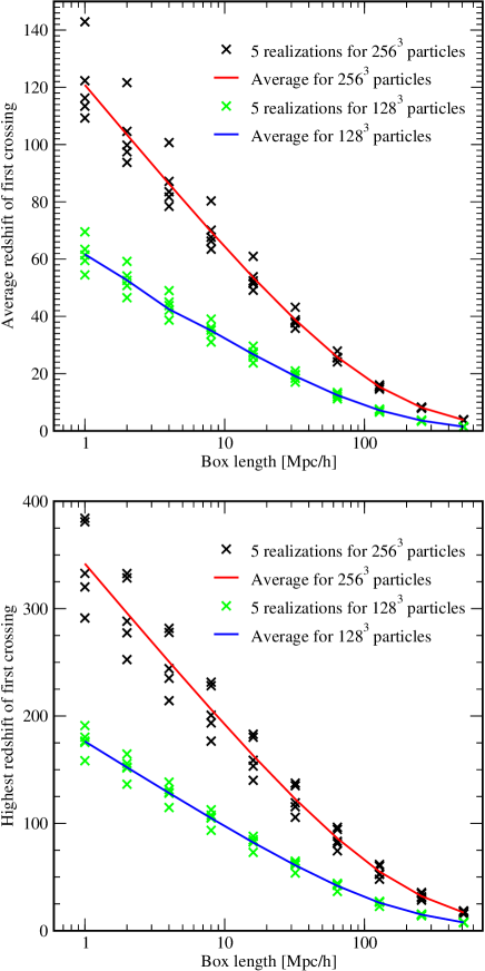
Figure 5: Average redshift of first crossing (top) and highest redshift of first crossing (bottom) as a function of box size. The initial conditions (five different realizations) are shown for boxes between 1 and 512$\,h^{-1}$Mpc with 128³ and 256³ particles. For each initial condition, $z_{\rm cross}^{\rm first}$ and $z_{\rm cross}^{\rm rms}$ are shown by the crosses. The solid lines show the average from the five realizations. As expected, scatter from the different realizations is larger for smaller boxes. These plots provide estimates of the required initial redshift for a simulation since $|\nabla\phi|/\Delta_{\rm p}$ is $z$-independent in the Zel’dovich approximation (see text).

In cosmological simulations, initial conditions are most often generated using the Zel’dovich approximation Zel’dovich (1970). Initially each particle is placed on a uniform grid or in a glass configuration and is then given a displacement determined by the relation

$${\bf x}={\bf q}-d(z)\nabla{\bf\phi},$$ (23)

where ${\bf q}$ is the Lagrangian coordinate of each particle. The gradient of the potential $\bf{\phi}$ is independent of the redshift $z$. The Zel’dovich approximation holds in the mildly nonlinear regime, as long as particle trajectories do not cross each other (no caustics have formed). Studying the magnitude of $|{\nabla\bf\phi}|$ allows us to estimate two important redshift values: first, the initial redshift $z_{\rm in}$ at which the particles should not have moved on average more than a fraction of the interparticle spacing $\Delta_{\rm p}=L_{\rm box}/n_{\rm p}$, where $L_{\rm box}$ is the physical box size and $n_{\rm p}$ the number of particles in the simulation; second, the redshift at which particles first move more than the interparticle spacing, $z_{\rm cross}$, i.e., at which they have traveled on average a distance greater than $\Delta_{\rm p}$.

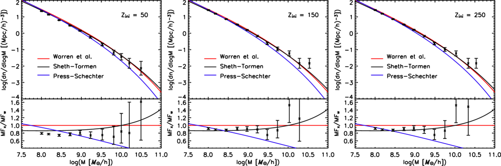
Figure 6: Dependence of the mass function on the initial redshift. The results are at $z=10$ from three 8$\,h^{-1}$Mpc box simulations with $z_{\rm in}=50$ (left), $z_{\rm in}=150$ (middle), and at $z_{\rm in}=250$ (right). The mass function in the left panel is systematically lower than the other two by roughly 15%. Poisson error bars are shown.

For a given realization of the power spectrum, the magnitude of $|{\nabla\bf\phi}|$ depends on two parameters: the physical box size and the interparticle spacing. Together these parameters determine the range of scales under consideration. The smaller the box, the smaller the scales; therefore, $|{\nabla\bf\phi}|$ increases and both $z_{\rm in}$ and $z_{\rm cross}$ increase. Increasing the resolution has the same effect. In Figure 4 we show the probability distribution function for $|{\nabla\phi}|$ for three different box sizes, $8$, $32$, and $126\,h^{-1}$Mpc, representing values studied by other groups, as well as in this paper. To make the comparison between the different box sizes more straightforward, we have scaled $|{\nabla\bf\phi}|$ with respect to the interparticle spacing $\Delta_{\rm p}$. All curves are drawn from simulations with 256³ particles on a 256³ grid, in accordance with the set up of our initial conditions. The behavior of the probability function follows our expectations: the smaller the box, or the higher the force resolution, the larger the initial displacements of the particles on average. From the mean and maximum values of such a distribution we can determine appropriate values for $z_{\rm in}$ and $z_{\rm cross}$. For our estimates we assume $d(z)\simeq 1/(1+z)$, which is valid for high redshifts. The maximum and rms initial displacements of the particles can then be easily calculated:

$$\delta^{\rm max}_{\rm in} \simeq \frac{{\rm max}(|\nabla\phi|/\Delta_{\rm p})}{1+z_{\rm in}},$$ (24)

$$\delta^{\rm rms}_{\rm in} \simeq \frac{{\rm rms}(|\nabla\phi|/\Delta_{\rm p})}{1+z_{\rm in}}.$$ (25)

The very first “grid crossing” of a particle occurs when $\delta^{\rm max}_{\rm in}=1$; on average the particles have moved more than one particle spacing when $\delta^{\rm rms}_{\rm in}=1$. This leads to the following estimates:

$$z^{\rm first}_{\rm cross} \simeq {\rm max}(\nabla\phi/\Delta_{\rm p})-1,$$ (26)

$$z^{\rm rms}_{\rm cross} \simeq {\rm rms}(\nabla\phi/\Delta_{\rm p})-1.$$ (27)

We show these two redshifts in Figure 5 for 10 different box sizes ranging from 1 to 512$\,h^{-1}$Mpc and for 256³ and 128³ particles. The top panel shows the average redshift of the first crossing as a function of box size (which corresponds to the maximum in Fig. 4). The bottom panel shows the redshift where the first “grid crossing” occurs (corresponding to the right tail in Fig. 4). To estimate the scatter in the results, we have generated five different realizations for each box. As expected, the small boxes show much more scatter. The average redshift of the first crossing in the 1$\,h^{-1}$Mpc box varies between $z=63$ and 83, while there is almost no scatter in the 512$\,h^{-1}$Mpc box. Since $|\nabla\phi|/\Delta_{\rm p}$ is independent of redshift in the Zel’dovich approximation, a simple scaling determines the appropriate initial redshift from these plots. For example, if a particle should not have moved more than 0.3$\Delta_{\rm p}$ on average at the initial redshift, the average redshift of first crossing has to be multiplied by a factor $1/0.3=3.\bar{3}$. For an $8\,h^{-1}$Mpc box this leads to a minimum starting redshift of $z=230$, while for a $126\,h^{-1}$Mpc box this suggests a starting redshift of $z_{\rm in}=50.$ The 128³ particle curve can be scaled to the 256³ particle curve by multiplying by a factor of 2. Curves for different particle loadings can be obtained similarly.

4.2 Transients and Mixing

The Zel’dovich approximation matches the exact density and velocity fields to linear order in Lagrangian perturbation theory. Therefore, there is in principle an error arising from the resulting discrepancy with the density and velocity fields given by the exact growing mode initialized in the far past.

This error is linear in the number of expansion factors between $z_{\rm in}$ and the redshift of interest $z_{\rm phys}$. It has been explored in the context of simulation error by Valageas (2002) and by Crocce et al. (2006). Depending on the quantity being calculated, the number of expansion factors between $z_{\rm in}$ and $z_{\rm phys}$ required to limit the error to some given value may or may not be easy to estimate. For example, unlike quantities such as the skewness of the density field, there is no analytical result for how this error impacts the determination of the mass function. Neither does there exist any independent means of validating the result aside from convergence studies. Nevertheless, it is clear that to be conservative, one should aim for a factor of $\sim 20$ in expansion factor in order to anticipate errors at the several percent level, a rule of thumb that has been followed by many $N$-body practitioners (and often violated by others!). This rule of thumb gives redshift starts that are roughly in agreement with the estimates in the previous subsection. Convergence tests done for our simulations show that the suppression in the mass function is very small (less than 1%) for simulations whose evolution covers a factor of 15 in the expansion factor and can be up to 20% for simulations that evolved by only 5 expansion factors. However, due to modest particle loads, we were unable to distinguish between the error induced by too few expansion factors and the breakdown of the Zel’dovich approximation.

Another possible problem, independent of the accuracy of the Zel’dovich approximation, is the initial particle distribution itself. Whether based on a grid or a glass, the small-distance ($k>k_{\rm Ny}$) mass distribution is clearly not sampled at all by the initial condition. Therefore, unlike the situation that would arise if a fully dynamically correct initial condition were given, some time must elapse before the correct small-separation statistics can be established in the simulation. Thus, all other things being equal, for the correct mass function to exist in the box, one must run the simulation forward by an amount sufficiently greater than the time taken to establish the correct small-scale power on first-halo scales while erasing memory on these scales of the initial conditions. If this is not done, structure formation will be suppressed, leading to a lowering of the halo mass function.

Because there is no fully satisfactory way to calculate $z_{\rm in}$ in order to compute the mass function at a given accuracy, we subjected every simulation box to convergence tests in the mass function while varying $z_{\rm in}$. The results shown in this paper are all converged to the sub-percent level in the mass function. We give an example of one such convergence test below.

4.2.1 Initial Redshift Convergence Study

As mentioned above, we have tested and validated our estimates for the initial redshift for all the boxes used in the simulation suite via convergence studies. Here, we show results for an 8$\,h^{-1}$Mpc box with initial redshifts $z_{\rm in}=50$, 150, and 250 in Figure 6, where the mass functions at $z=10$ are displayed. For the lowest initial redshift, $z_{\rm in}=50$, the average initial particle movement is 1.87$\Delta_{\rm p}$, while some particles travel as much as 5.03$\Delta_{\rm p}$. This clearly violates the requirement that the initial particle grid distortion be kept sufficiently below 1 grid cell. The starting redshift $z_{\rm in}=150$ leads to an average displacement of 0.63$\Delta_{\rm p}$ and a maximum displacement of 1.71$\Delta_{\rm p}$, and therefore just barely fulfills the requirements. For $z_{\rm in}=250$ we find an average displacement in this particular realization of 0.37$\Delta_{\rm p}$ and a maximum displacement of 1.00$\Delta_{\rm p}$.

The bottom plot in each of the three panels of Figure 6 shows the ratio of the mass functions with respect to the Warren fit. In the middle and right panels the ratio for the largest halo is outside the displayed range. The mass function from the simulation started at $z_{\rm in}=50$ (left panel) is noticeably lower, $\sim 15\%$, than for the other two simulations. The mass functions from the two higher redshift starts are in good agreement, showing that the choice for average grid distortion of approximately 0.3$\Delta_{\rm p}$ is conservative, and that one can safely use (0.5–0.6)$\Delta_{\rm p}$. The general conclusion illustrated by Figure 6 is that if a simulation is started too late, halos are found to be missing over the entire mass range. With the late start, there is less time to form bound objects. Also, some particles that are still streaming towards a halo do not have enough time to join it. Both of these artifacts lead to an overall downshift of the mass function.

To summarize, requiring a limit on initial displacements sets the starting redshift much higher than simply demanding that all modes in the box stay linear. Indeed, the commonly used latter criterion (with $\delta^{\rm rms}\sim 0.1$) is not adequate for computing the halo mass function at high redshifts. One must verify that the chosen $z_{\rm in}$ sets an early enough start as shown here. We comment on previous results from other groups with respect to this finding below in §6.

4.3 Force and Mass Resolution

We now take up an investigation of the mass and force resolution requirements. The first useful piece of information is the size of the simulation box: from Figure 2 we can easily translate the number density into when the first halo is expected to appear in a box of volume $V$. For example, a horizontal line at $n=10^{-6}$ would tell us at what redshift we would expect on average to find 1 halo of a certain mass in a $(100\,h^{-1}$Mpc)³ box. The first halo of mass $~{}10^{11}-10^{12}\,h^{-1}M_{\odot}$ will appear at $z\simeq 15.5$, and the first cluster-like object of mass $~{}10^{14}-10^{15}\,h^{-1}M_{\odot}$ at $z\simeq 2$. Of course, these statements only hold if the mass and force resolution are sufficient to resolve these halos. The mass of a particle in a simulation, and hence the halo mass, is determined by three parameters: the matter content of the Universe $\Omega_{\rm m}$, including baryons and dark matter, the physical box size $L_{\rm box}$, and the number of simulation particles $n_{\rm p}^{3}$:

$$m_{\rm particle}=2.775\times 10^{11}\Omega_{\rm m}\left(\frac{L_{\rm box}}{n_{\rm p}\,h^{-1}{\rm Mpc}}\right)^{3}\,h^{-1}{M}_{\odot}.$$ (28)

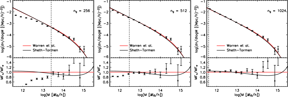
Figure 7: Convergence of the mass function as a function of force resolution. All results are shown at $z=0$, for 256³ particles and a 126$\,h^{-1}$Mpc box with Poisson error bars. The resolution varies between 256³ (left), 512³ (middle), and 1024³ grid points (right). The vertical line denotes the predicted theoretical resolution limit: halos on the right of the line should not be lost. The resolution limit is 2500 particles per halo for the 256³ grid, 300 particles per halo for the $512^{3}$ grid, and 40 particles per halo for the 1024³ grid.

The required force resolution to resolve the chosen smallest halos can be estimated very simply. Suppose we aim to resolve a virialized halo with comoving radius $r_{\Delta}$ at a given redshift $z$, where $\Delta$ is the overdensity parameter with respect to the critical density $\rho_{\rm c}$. The comoving radius $r_{\Delta}$ is given by

$$r_{\Delta}=9.51\times 10^{-5}\left[\frac{\Omega(z)}{\Omega_{\rm m}}\right]^{1/3}\left(\frac{1}{\Delta}\frac{M_{\Delta{\rm c}}}{h^{-1}{\rm M_{\odot}}}\right)^{1/3}\,h^{-1}{\rm Mpc},$$ (29)

where $\Omega(z)=\Omega_{\rm m}(1+z)^{3}/[\Omega_{\rm m}(1+z)^{3}+\Omega_{\Lambda}]$ and the halo mass $M_{\Delta{\rm c}}=m_{\rm part}n_{\rm h}$, where $n_{\rm h}$ is the number of particles in the halo. We measure the force resolution in terms of

$$\delta_{\rm f}=\frac{L_{\rm box}}{n_{\rm g}}.$$ (30)

In the case of a grid code, $n_{\rm g}$ is literally the number of grid points per linear dimension; for any other code, $n_{\rm g}$ stands for the number of “effective softening lengths” per linear dimension. To resolve halos of mass $M_{\Delta{\rm c}}$, a minimal requirement is that the code resolution be smaller than the radius of the halo we wish to resolve:

$$\delta_{\rm f}<r_{\Delta}.$$ (31)

Note that this minimal resolution requirement is aimed only at capturing halos of a certain mass, not at resolving their interior profile. Next, inserting the expression for the particle mass (eq. [28]) and the comoving radius (eq. [29]) into the requirement (eq [31]) and employing the relation between the interparticle spacing $\Delta_{\rm p}$ and the box size $\Delta_{\rm p}=L_{\rm box}/n_{\rm p}$, the resolution requirement reads

$$\frac{\delta_{\rm f}}{\Delta_{\rm p}}<0.62\left[\frac{n_{h}\Omega(z)}{\Delta}\right]^{1/3}.$$ (32)

We now illustrate the use of this simple relation with an example. Let $\Delta=200$ and consider a $\Lambda$CDM cosmology with $\Omega_{\rm m}=0.3$. Then for PM codes for which $\delta_{\rm f}/\Delta_{\rm p}=n_{\rm p}/n_{\rm g}$, we have the following conclusions. If the number of mesh points is the same as the number of particles ($n_{\rm p}=n_{\rm g}$), halos with less than 2500 particles cannot be accurately resolved. If the number of mesh points is increased to 8 times the particle number ($n_{\rm p}=1/2n_{\rm g}$), commonly used for cosmological simulations with PM codes, the smallest halo reliably resolved has roughly 300 particles, and if the resolution is increased to a ratio of 1 particle per 64 grid cells, which we use in the main PM simulations in this paper, halos with roughly 40 particles can be resolved. It has been shown in Heitmann et al. (2005) that this ratio (1:64) does not cause collisional effects and that it leads to consistent results in comparison to high-resolution codes. Note that increasing the resolution beyond this point will not help, since it is unreliable to sample halos with too few particles. Note also that a similar conclusion holds for any simulation algorithm and not just for PM codes.

In Figure 7 we show results from a resolution convergence test at $z=0$. We run 256³ particles in a 126$\,h^{-1}$Mpc box with three different resolutions: 0.5, 0.25, and 0.125$\,h^{-1}$Mpc. The vertical line in each figure shows the mass below which the resolution is insufficient to capture all halos following condition (32). In all three cases, the agreement with the theoretical prediction is excellent.

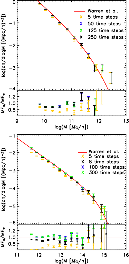
Figure 8: Top: One of the 32$\,h^{-1}$Mpc box realizations run with 250, 125, 50 and 5 time steps between $z_{\rm in}=150$ and $z_{\rm final}=5$. The mass function is shown at the final redshift $z=5$. Data points for all runs except the one with five time steps are so close that they are difficult to distinguish. Bottom: A 126$\,h^{-1}$Mpc box with 300, 100, 8, and 5 time steps between $z_{\rm in}=50$ and $z_{\rm final}=0$. The agreement for the very large halos for 100 and 300 time steps is essentially perfect. Poisson error bars are shown.

4.4 Time Stepping

Next, we consider the question of time-step size and estimate the minimal number of time steps required to resolve the halos of interest. We begin with a rough estimate of the characteristic particle velocities in halos. For massive halos, the halo mass $M_{200}$ and its velocity dispersion are connected by the approximate relation (Evrard 2004):

$$M_{200}\simeq\frac{10^{15}\,h^{-1}M_{\odot}}{H/H_{0}}\left(\frac{\sigma_{v}}{1080{\rm\,km/s}}\right)^{3}.$$ (33)

A more accurate expression can be found in Evrard et al. (2007), but the above is more than sufficient for our purposes. At high redshift, $\Omega_{\Lambda}$ can be neglected, and we can express the velocity dispersion as a function of redshift:

$$\sigma_{\rm v}\simeq 10^{-2}\sqrt{1+z}\left(\frac{M_{200}}{\,h^{-1}M_{\odot}}\right)^{1/3}{\rm kms^{-1}}.$$ (34)

In a time $\delta t$, the characteristic scale length $\delta l$ is given by $\delta l\simeq\sigma_{\rm v}\delta t$ or

$$\delta t\simeq\frac{\delta l}{\sigma_{v}}=\frac{100\,\delta l/{\rm km}}{\sqrt{1+z}}\left(\frac{M_{200}}{\,h^{-1}M_{\odot}}\right)^{-1/3}{\rm s}.$$ (35)

The scale factor $a$ is a convenient time variable for codes working in comoving units, such as ours. Expressed in terms of the scale factor, equation (35) reads:

$$\delta a\simeq 10^{4}\frac{\delta l}{h^{-1}{\rm Mpc}}\left(\frac{M_{200}}{h^{-1}M_{\odot}}\right)^{-1/3}.$$ (36)

We are interested in the situation where $\delta l$ is actually the force resolution, $\delta_{\rm f}$. In a single time step, the distance moved should be small compared to $\delta_{\rm f}$; i.e., the actual time step should be smaller than $\delta a$ estimated from the above equation when $\delta l$ is replaced on the right–hand side with $\delta_{\rm f}$. Let us consider a concrete example for the case of a PM code where $\delta_{\rm f}=L_{\rm box}/n_{\rm g}$ as explained earlier. For a “medium” box size of $L_{\rm box}=256\,h^{-1}{\rm Mpc}$ and a grid size of $n_{\rm g}=1024$, $\delta_{\rm f}=0.25\,h^{-1}{\rm Mpc}$. For a given box, the highest mass halos present have the largest $\sigma_{\rm v}$ and give the tightest constraints on the time step. For the chosen box size, a good candidate halo mass scale is $M_{200}\sim 10^{15}\,h^{-1}M_{\odot}$ (this could easily be less, but it does not change the result much). In this case,

$$\delta a\simeq 0.025.$$ (37)

If, for illustration, we start a simulation at $z=50$ and evolve it down to $z=0$, this translates to roughly 40 time steps. We stress that this estimate is aimed only at avoiding disruption of the halos themselves, and is certainly not sufficient to resolve the inner structure of the halo.

In Figure 8 we show two tests of the time step criterion. The top panel shows the result from a 32$\,h^{-1}$Mpc box at redshift $z=5$. The simulation starts at $z_{\rm in}=150$ and is evolved with 50, 125, and 250 time steps down to $z=5$. Following the argument above for this box size, one would expect all three choices to be acceptable, and the excellent agreement across these runs testifies that this is indeed the case. We also carried out a run with only five time steps, which yields a clearly lower ($\sim 20\%$) mass function than the others, but not as much as one would probably expect from such an imprecise simulation.

The bottom panel shows the results from a 126$\,h^{-1}$Mpc box at $z=0$. This simulation was started at $z{\rm in}=50$ and run to $z=0$ with 5, 8, 100, and 300 time steps. Again, as we would predict, the agreement is very good for the last two simulations, and the convergence is very fast, confirming our estimate that only ${\cal{O}}(10)$ time steps is enough to get the correct halo mass function. Overall, the halo mass function appears to be a very robust measure, not very sensitive to the number of time steps. Nevertheless, we used a conservatively large number of time steps, e.g., 500 for the simulations stopping at $z=0$ and 300 for those stopping at $z=10$.

In the previous subsections we have discussed and tested different error control criteria for obtaining the correct simulated mass function at all redshifts. These criteria are (1) a sufficiently early starting redshift to guarantee the accuracy of the Zel’dovich approximation at that redshift and provide enough time for the halos to form; (2) sufficient force and mass resolution to resolve the halos of interest at any given redshift; and (3) sufficient numbers of time steps. Violating any of these criteria always leads to a suppression of the mass function. Most significantly, our tests show that a late start (i.e., starting redshift too low) leads to a suppression over the entire mass range under consideration, and is a likely explanation of the low mass function results in the literature. As intuitively expected, insufficient force resolution leads to a suppression of the mass function at the low-mass end, while errors associated with time stepping are clearly subdominant and should not be an issue in the vast majority of simulations.

5 Results and Interpretation

In this section we present the results from our simulation suite. We describe how the data are obtained as well as the post-processing corrections applied. The latter include compensation for FOF halo mass bias induced by finite (particle number) sampling, and the (small) systematic suppression of the mass function induced by the finite volume of the simulation boxes.

5.1 Binning of Simulation Data

Before venturing into the simulation results, we first describe how they were obtained and reported from individual simulations. We used narrow mass bins while conservatively keeping the statistical shot noise of the binned points no worse than some given value. Bin widths $\Delta\log M$ were chosen such that the bins contain an equal number of halos $N_{\rm h}$. The worst-case situation occurs at $z=20$ for the 8$\,h^{-1}$Mpc box, which has $N_{\rm h}=80$; the 4$\,h^{-1}$Mpc box at the same redshift has $N_{\rm h}=400$. At $z=15$ we have $N_{\rm h}=150$, 1600, and 3000 for box sizes 16, 8, and 4$\,h^{-1}$Mpc, respectively. At $z=10$ the smallest value $N_{\rm h}=450$ is for the 32$\,h^{-1}$Mpc box, while at $z=5$ and 0 we essentially always have $N_{\rm h}>10000$.

With a mass function decreasing monotonically with $M$, this binning strategy results in bin widths increasing monotonically with $M$. The increasing bin size may cause a systematic deviation – growing towards larger masses – from an underlying “true” continuous mass function. The data points for the binned mass function give the average number of halos per volume in a bin,

$$\bar{F}\equiv N_{\rm h}/(V\Delta\log M),$$ (38)

plotted versus an average halo mass, averaged by the number of halos in the bin:

$$\bar{M}\equiv\sum_{\rm bin}M/N_{\rm h}.$$ (39)

Assuming that the true mass function $dn/d\log M$ has some analytic form $F(M)$, a systematic deviation due to the binning prescription

$$\epsilon_{\rm{bin}}\equiv\frac{\bar{F}-F(\bar{M})}{F(\bar{M})}$$ (40)

can be evaluated by computing $\bar{F}$ and $\bar{M}$ as

$$\bar{F}=\frac{\int_{\Delta M}dn}{\Delta\log M},~{}~{}~{}\bar{M}=\frac{\int_{\Delta M}Mdn}{\int_{\Delta M}dn},$$ (41)

where $dn\equiv F(M)\,d\log M$ and the integrations are over a mass range $[M,M+\Delta M]$. For the leading-order term of the Taylor expansion of $\epsilon_{\rm bin}(\Delta M)$, we find

$$\epsilon_{\rm{bin}}\simeq\frac{F^{\prime\prime}-2(F^{\prime})^{2}/F}{24F}(\Delta M)^{2},$$ (42)

where the primes denote $\partial/\partial M$. A characteristic magnitude of this $\epsilon_{\rm bin}$ for a general $F(M)$ is $(\Delta M/M)^{2}/24$. However, in our case, where the relevant scales $k\gg k_{\rm eq}\sim 0.01h$Mpc^-1, $\epsilon_{\rm bin}$ has a much stronger suppression, as explained below.

We know that the mass function is close to the universal form,

$$F(M)=\frac{\rho_{\rm b}}{M}f(\sigma)\frac{d\ln\sigma^{-1}}{d\log M}$$ (43)

(see, eq. [1]). Note that for $k\gg k_{\rm eq}$, $\sigma^{-1}(M)$ is a slowly varying function, i.e.,

$$\frac{d\log\sigma^{-1}}{d\log M}\equiv\frac{n_{\rm eff}+3}{6}$$ (44)

is much smaller than unity, and the derivative $d\log\sigma^{-1}/d\log M$ also changes slowly with $M$. Then, despite the steepness of $F(\sigma)$ at small $\sigma$, the factor $f(\sigma)\,d\ln\sigma^{-1}/d\log M$ in equation (43) depends weakly on $M$. Therefore, the mass function $F(M)$ is close to being inversely proportional to $M$. In the limit of exact inverse proportionality, $F\propto M^{-1}$, equation (42) tells us that $\epsilon_{\rm{bin}}\rightarrow 0$. This effective cancellation of the two terms on the right-hand side of equation (42) makes the binning error negligible to the accuracy of our $F(M)$ reconstruction whenever a bin width $\Delta\log M$ does not exceed $0.5$. To confirm the absence of any systematic offsets due to the binning, we binned the data into $\log M$ intervals 5 times narrower and wider, with no apparent change in the inferred $F(M)$ dependence.

We remark that the situation could be quite different with another binning choice. For example, if the binned masses $\bar{M}$ were chosen at the centers of the corresponding $\log M$ intervals, $\log\bar{M}=[\log M+\log(M+\Delta M)]/2$, the systematic binning deviation

$$\epsilon_{\rm{bin}}^{({\rm center})}\simeq\frac{F^{\prime\prime}+F^{\prime}/M}{24F}(\Delta M)^{2}$$ (45)

would have no special cancellation for the studied type of mass function. A corresponding binning error would be about 2 orders of magnitude larger than that of equations (38) and (39).

The statistical error bars used are Poisson errors, following the improved definition of Heinrich (2003):

$$\sigma_{\pm}=\sqrt{N_{\rm h}+\frac{1}{4}}\pm\frac{1}{2}.$$ (46)

At large values of $N_{h}$, these error bars asymptote to the familiar form $\sqrt{N}_{\rm h}$. At smaller values of $N_{\rm h}$ – which are of minor concern here – equation 46 has several advantages over the standard Poisson error definition, some being (1) it is nonzero for $N_{\rm h}=0$; (2) the lower edge of the error bar does not go all the way to zero when $N_{\rm h}=1$; (3) the asymmetry of the error bars reflects the asymmetry of the Poisson distribution.

Finally, as noted earlier and discussed in the next section, all the results shown in the following include a correction for the sampling bias of FOF halos according to equation (47). This mass correction brings down the low-mass end of the mass function.

5.2 FOF Mass Correction

Figure 9: FOF mass correction for halos in 4 (dark blue), 8 (black), 16 (light blue), and 32 (yellow) $h^{-1}$Mpc boxes. To show the effect clearly, we plot the ratio of our data to the Warren fit. Crosses show the uncorrected mass function and squares the mass function after correction, following eq. (47). Note the smooth behavior of the corrected mass function as opposed to the mass-function jumps across box sizes for the uncorrected data.

The mass of a halo as determined by the FOF algorithm displays a systematic bias with the number of particles used to sample the halo. Too few particles lead to an increase in the estimated halo mass. By systematically subsampling a large halo population from N-body simulations (at $z=0$), Warren determined an empirical correction for this undersampling bias. For a halo with $n_{\rm h}$ particles, his correction factor for the FOF mass is given by

$$n_{\rm h}^{\rm corr}=n_{\rm h}\left(1-n_{\rm h}^{-0.6}\right).$$ (47)

We have carried out an independent exercise to check the systematic bias of the FOF halo mass as a function of particle number based on Monte Carlo sampling of an NFW halo mass profile with varying concentration and particle number, as well as by direct checks against simulations (e.g., Fig. 9); our results are broadly consistent with equation (47). Details will be presented elsewhere (Z. Lukić et al., in preparation). In this associated work we also address how overdensity masses connect to FOF masses, how this relation depends on the different linking length used for the FOF finder, and the properties of the halo itself, such as the concentration.

The effect of the FOF sampling correction can be quickly gauged by considering a few examples: for a halo with 50 particles, the mass reduction is almost 10%, for a halo with 500 particles, it is $\sim 2.4\%$, and for a well-sampled halo with 5000 particles, it is only 0.6%. As a cautionary remark, this correction formula does not represent a general recipe but can depend on variables such as the halo concentration. Since the conditions under which different simulations are carried out can differ widely, corrections of this type should be checked for applicability on a case-by-case basis. Note also that the correction for the mass function itself depends on how halos move across mass bins once the FOF correction is taken into account.

The choice of the mass function range in a given simulation box always involves a compromise: too wide a dynamic range leads to poor statistics at the high-mass end and possible volume-dependent systematic errors, and too narrow a range leads to possible undersampling biases. Our choice here reflects the desire to keep good statistical control over each mass bin at the expense of wide mass coverage, compensating for this by using multiple box sizes. Therefore, in our case it is important to demonstrate control over the FOF mass bias. An example of this is shown in Figure 9, where results from four box sizes demonstrate the successful application of the Warren correction to simulation results at $z=10$.

5.3 Simulation Mass and Growth Function

The complete set of simulations, summarized in Table 2, allows us to study the mass function spanning the redshift range from $z=20$ to 0. The mass range covers dwarf to massive galaxy halos at $z=0$ (cluster scales are best covered by much bigger boxes as in Warren and Reed et al. 2007), and at higher redshifts goes down to $10^{7}\,h^{-1}M_{\odot}$, the mass scale above which gas in halos can cool via atomic line cooling (Tegmark et al. 1997).

5.4 Time Evolution of the Mass Function

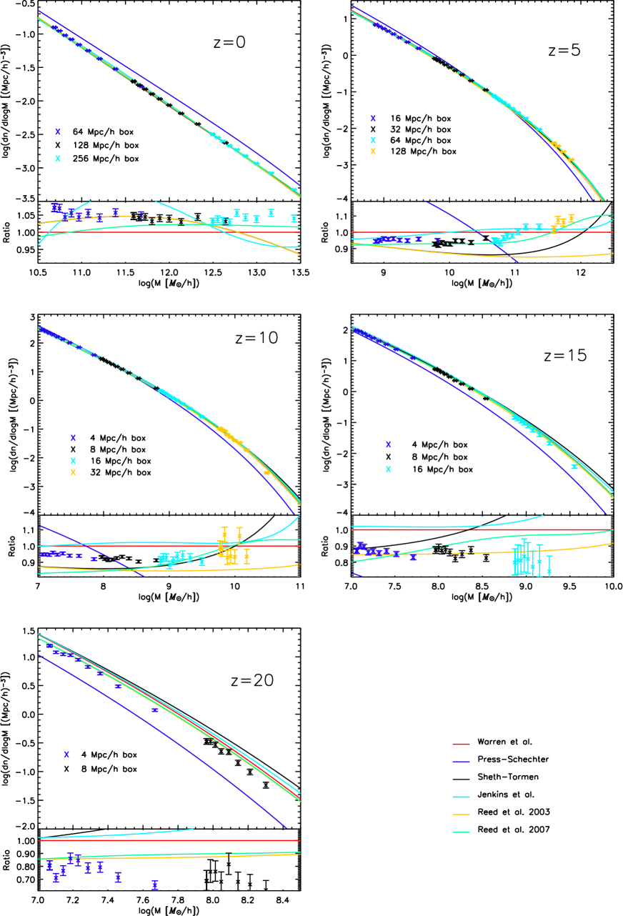
Figure 10: Mass function at five different redshifts ($z=0$, 5, 10, 15, and 20; top to bottom) compared to different fitting formulae. Note that the mass ranges are different at different redshifts. The simulation results have been corrected for FOF bias following Warren but not for finite-volume effects (for these, see Fig. 12). The bottom panel shows the ratio with respect to the Warren fit. Our simulations agree with the Warren fit at the 10% level for redshifts smaller than 10, although there is a systematic offset of 5% at $z=0$, where our numerical results are higher than the fit. At higher redshifts, the agreement is still very good (at the 20% level) and becomes very close once finite-volume corrections are applied (Fig. 12). PS is a bad fit at all redshifts, and especially at high redshifts, where the difference between PS and the simulation results is an order of magnitude.

Halo mass functions from the multiple-box simulations are shown in Figure 10, with results being reported at five different redshifts with no volume corrections applied. The combination of box sizes is necessary because larger boxes do not have the mass resolution to resolve very small halos at early redshifts, while smaller boxes cannot be run to low redshifts. The bottom plot of each panel shows the ratio of the numerically obtained mass function, and various other fits, to the Warren fit as scaled by linear theory (for volume-corrected results, see Fig. 12). Displaying the ratio has the advantage over showing relative residuals that large discrepancies (more than 100%) appear more clearly. For all redshifts, the agreement with the Warren fit is at the 20% level. The ST fit matches the simulations for small masses very well but overpredicts the number of halos at large masses. This overprediction becomes worse at higher redshifts. For example, at $z=15$ ST overpredicts halos of 10${}^{9}\,h^{-1}M_{\odot}$ by a factor of 2. Reed et al. (2003) found a similar result: the ST fit at $z=15$ for halos with mass larger than $10^{10}\,h^{-1}M_{\odot}$ disagrees with their simulation by 50%. Agreement with the Reed et al. (2003, 2007) fits is also good, within the 10% level. (For a further discussion focused around the question of universality, see Section 5.7.) The PS fit in general is not satisfactory over a larger mass range at any redshift. It crosses the other fits at different redshifts for different masses. Away from this crossing region, however, the disagreement can be as large as an order of magnitude, e.g. for $z=20$ over the entire mass range we consider here.

5.5 Halo Growth Function

As discussed in §2.4 the halo growth function (the number density of halos in mass bins as a function of redshift) offers an alternative avenue to study the time evolution of the mass function. Figure 11 shows the halo growth function for an 8$\,h^{-1}$Mpc box for three different starting redshifts, $z_{\rm in}=50$, 150, and 250 (these are the same simulations as in Fig. 6). The results are displayed at three redshifts, $z=20$, 15, and 10 and for three mass bins, $10^{8}-10^{9}\,h^{-1}M_{\odot}$, $10^{9}-10^{10}\,h^{-1}M_{\odot}$, and $10^{10}-10^{11}\,h^{-1}M_{\odot}$.

Assuming that the Warren fit scales at least approximately to high redshifts, the first halos in the lowest mass bin are predicted to form at $z_{\rm form}\sim 25$ (see Fig. 6). We have found that if $z_{\rm form}$ is not sufficiently far removed from $z_{\rm in}$, formation of the first halos is significantly delayed/suppressed. In turn, this leads to suppressions of the halo growth function and the mass function at high redshifts. As shown in Figure 11, the suppression can be quite severe at high redshifts: the simulation result at $z=20$ from the late start at $z_{\rm in}=50$ is an order of magnitude lower than that from $z_{\rm in}=250$. At lower redshifts, the discrepancy decreases, and results from late-start simulations begin to catch up with the results from earlier starts. Coincidentally, the suppression due to the late start at $z_{\rm in}=50$ is rather close to the PS prediction which is very significantly below the Warren fit in the mass and redshift range of interest (see Fig. 11). We take up this point further below.

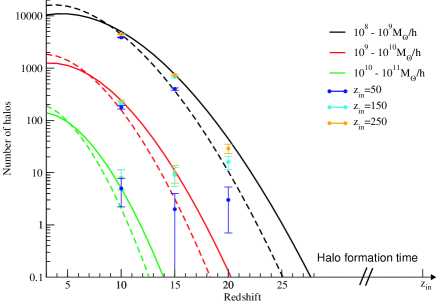
Figure 11: Halo growth function for an 8$\,h^{-1}$Mpc box started from three different redshifts. The blue data points results from the $z=50$ start, the turquoise data points from the $z=150$ start, and orange from the $z=250$ start, which is the redshift satisfying our starting criteria. The two fits shown are the Warren fit (solid line) and the PS fit (dashed line). Three different mass bins are shown. It is interesting to note that the late start seems to follow the PS fit at high redshift.

5.6 Finite-Volume Corrections

The finite size of simulation boxes can compromise results for the mass function in multiple ways. It is important to keep in mind that finite-volume boxes cannot be run to lower than some redshift, $z_{\rm final}$, the stopping point being determined by when nonlinear scales approach close enough to the box size. Approaching too near this point delays the ride-up of nonlinear power towards the low-$k$ end, with a possible suppression of the mass function.

As a consequence of this delay, the evolution (incorrectly) appears more linear at large scales than it actually should, as compared to the $P(k)$ obtained in a much bigger box. Therefore, verifying linear evolution of the lowest $k$-mode is by itself not sufficient to establish that the box volume chosen was sufficiently large. For all of our overlapping-volume simulations we have checked that the power spectra were consistent across boxes up to the lowest redshift from which results have been reported (Table 1 lists the stopping redshifts).

Aside from testing for numerical convergence, it is important to show that finite-volume effects are also under control, especially any suppression of the mass function with decreasing box size (due to lack of large-scale power on scales greater than the box size). Several heuristic analyses of this effect have appeared in the literature. Rather than rely solely on the unknown accuracy of these results, however, here we also numerically investigate possible systematic differences in the mass function with box size.

Over the redshifts and mass ranges probed in each of our simulation boxes, we find no direct evidence for an error caused by finite volume (at more than the $\sim 20\%$ level), as already emphasized previously in Heitmann et al. (2006a). (Overlapping box-size results over different mass ranges are shown in Fig. 3 of Heitmann et al. 2006a.) Figure 10 shows the corresponding results in the present work. This is not to say that there are no finite-volume effects (the very high-mass tail in a given box must be biased low simply from sampling considerations) but that their relative amplitude is small. Below we discuss how to correct the mass function for finite box size.

5.6.1 Volume Corrections from Universality

Let us first assume that mass function universality holds strictly, in other words, that for any initial condition the number of halos can be described by a certain scaled mass function (eq. [1]) in which $\sigma(M)$ is the variance of the top-hat-smoothed linear density field. In the case of infinite simulation volume, $\sigma(M)$ is determined by equation (3), and the mass function $F(M)$ of equation (2) is

$$F(M)\equiv{dn\over d\log M}=\frac{\rho_{b}}{M}f(\sigma)\frac{d\ln\sigma^{-1}}{d\log M}\ .$$ (48)

In an ensemble of finite-volume boxes, however, one necessarily measures a different quantity:

$$F^{\prime}(M^{\prime})\equiv{dn^{\prime}\over d\log M^{\prime}}=\frac{\rho_{b}}{M^{\prime}}f(\sigma^{\prime})\frac{d\ln\sigma^{\prime-1}}{d\log M^{\prime}}\ .$$ (49)

Here $\sigma^{\prime}(M^{\prime})$ is determined by the (discrete) power spectrum of the simulation ensemble, although if universality holds as assumed, $f$ in equations (48) and (49) is the same function.

Since we are, in general, interested in the mass function which corresponds to an infinite volume, we can then correct the data obtained from our simulations as follows: for each box size we can define a function $M^{\prime}(M)$ such that

$$\sigma(M)\equiv\sigma^{\prime}(M^{\prime}(M)).$$ (50)

Using equations (48) – (50), we determine $F(M)$ as

$$F(M)=F^{\prime}(M^{\prime})\,\frac{dM^{\prime}(M)}{dM}.$$ (51)

Thus, the corrected number of halos in each bin is calculated as

$$dn=dn^{\prime}\frac{M^{\prime}}{M}\ .$$ (52)

The universality must eventually break down for sufficiently small boxes or high accuracy because the nonlinear coupling of modes is more complicated than that described by the smoothed variance. This violation can be partly corrected for by modifying the functional form of $\sigma^{\prime}(M^{\prime})$. Therefore, we also explore other choices of $\sigma^{\prime}(M^{\prime})$ which may better represent the mass function in the box. To address this question we provide a short summary of the Press-Schechter approach.

5.6.2 Motivation from Isotropic Collapse

We first consider the idealized case of a random isotropic perturbation of pressureless matter and assume that the primordial overdensity at the center of this perturbation has a Gaussian probability distribution. The probability of local matter collapse at the center is then fully determined by the local variance of the primordial overdensity $\sigma^{2}$. Consequently, for the isotropic case the contribution of Fourier modes of various scales to the collapse probability is fully quantified by their contribution to $\sigma^{2}$.

To see this, consider the evolution of matter density $\rho_{\rm loc}$ at the center of the spherically symmetric density perturbation. For transparency of argument, let us focus on the evolution during the matter-dominated era; it is straightforward to generalize the argument to include a dark energy component $\rho_{\rm de}(z)$, homogeneous on the length scales of interest, by a substitution $\rho_{\rm loc}\to\rho_{\rm m,\,\rm loc}+\rho_{\rm de}$ in equations (53) and (55). By Birkhoff’s law, the evolution of $\rho_{\rm loc}$ and the central Hubble flow $H_{\rm loc}\equiv\frac{1}{3}\bm{\nabla}\cdot\bm{v}_{\rm loc}$ are governed by the closed set of the Friedmann and conservation equations,

$$H_{\rm loc}^{2} = \frac{8\pi G\rho_{\rm loc}}{3}-\frac{\kappa}{a_{\rm loc}^{2}},$$ (53)

$$a_{\rm loc} \equiv \left(\frac{\rho_{0}}{\rho_{\rm loc}}\right)^{1/3},~{}~{}\frac{da_{\rm loc}}{dt}=H_{\rm loc}a_{\rm loc},$$ (54)

where $\kappa$ is a constant determined by the initial conditions, $\rho_{0}$ is arbitrary (e.g., $\rho_{0}=\left.\rho_{b}\right|_{z=0}$), and $t$ is the proper time.

The degree of nonlinear collapse at the center can be quantified by a dimensionless parameter

$$q\equiv 1-\frac{3H_{\rm loc}^{2}}{8\pi G\rho_{\rm loc}}.$$ (55)

First consider early times, when the evolution is linear, and let $\rho_{\rm loc}=\rho_{b}(1+\delta)$. Then for the growing perturbation modes during matter domination $H_{\rm loc}=\bar{H}(1-\delta/3)$. Given these initial conditions, which set the initial $\rho_{\rm loc}$ and the constant $\kappa$ in equation (53), the subsequent evolutions of $\rho_{\rm loc}$, $H_{\rm loc}$, and therefore $q$ are determined unambiguously.

During the linear evolution in the matter era $q=5\delta/3$ is small and grows proportionally to the cosmological scale factor $a$. For positive overdensity, nonlinear collapse begins when $q$ becomes of order unity, reaching its maximal value $q=1$ when $H_{\rm loc}=0$, and decreasing rapidly afterwards. (We can observe the latter by rewriting eq. [55] as

$$q=\frac{3\kappa}{8\pi Ga_{\rm loc}^{2}\rho_{\rm loc}}\propto\rho_{\rm loc}^{-1/3},$$ (56)

having applied eqs. [53] and [54].) Nonlinear collapse of matter at the center of the considered region can be said to occur either when $q\rightarrow 0$ or when $q$ reaches a critical “virialization” value $q_{c}$.

Now it is easy to argue that in the isotropic case the Press-Schechter approach gives the true probability of the collapse, $P(q>q_{c},z)$, for a redshift $z$. Indeed, the evolution of $q$ is set deterministically by the primordial density perturbation at the center; for adiabatic initial conditions specifically, it is set by the curvature perturbation $\zeta$ at the center. Since higher values of $\zeta$ lead to earlier collapse,

$$P(q>q_{c},z)=P(\zeta>\zeta_{c}(z))=\frac{1}{2}\mathop{\rm erfc}\left[\frac{\zeta_{c}(z)}{\sqrt{2}\,\sigma}\right],$$ (57)

where the last equality uses the explicit form of $P(\zeta)$ as a Gaussian distribution with a variance $\sigma^{2}$.

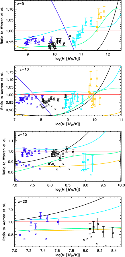
Figure 12: Mass function data corrected for finite box volume by the extended Press-Schechter prescription of §5.6.3 (squares). We show the results as a ratio with respect to the Warren fit and follow the conventions of Fig. 10. We also display the volume-uncorrected data (crosses). Note that the volume-corrected data join smoothly across the box-size boundaries. This box correction brings the results very close to universal behavior at high redshifts (see Fig.15).

If the considered isotropic distribution is confined by a (spherical) boundary and $\sigma$ at the center is reduced by removal of large-scale power, then equation (57) should accurately describe the corresponding change of the collapse probability. In numerical simulations, due to the imposition of periodic boundary conditions, there is no power on scales larger than the box size. In this case the variance $\sigma$ should be specified by the analogue of equation (3) with the integral replaced by a sum over discrete modes.

For the mass function (eq. [48]), a constant reduction of the variance $\sigma^{2}(M)$ due to the removal of large-scale power leads to a suppression of the mass function at the high-mass end and, counterintuitively, a boost at the low-mass end. The latter is easily understood as follows: The $\sigma$-dependent terms of equation (48),

$$f(\sigma)\frac{d\ln\sigma^{-1}}{d\log M}=\frac{d\rho(M)/\rho_{b}}{d\log M},$$ (58)

give the fraction of the total matter density that belongs to the halos of mass $M$. When the variance is decreased by the box boundaries, this fraction is boosted at low masses due to a shift of halo formation to an earlier stage, where a larger fraction of matter is bound into low-mass objects.

5.6.3 Numerical Results and Comparisons

Following the above intuition, we employ the extended Press-Schechter formalism (Bond et al. 1991) to correct for the missing fluctuation variance on box scales. This formalism, while clearly inadequate at various levels in describing halo formation in realistic simulations (Bond et al. 1991; Katz et al. 1993; White 1996), has nevertheless been very successful as a central engine in describing the statistics of cosmological structure formation. As shown by Mo & White (1996) using $N$-body simulations, the biasing of halos in a spherical region with respect to the average mass overdensity in that region is very well described by the extended Press-Schechter approach. Barkana & Loeb (2004) discussed the suppression of the halo mass function in terms of this bias, and suggested a prescription for adjusting large-volume mass function fits such as Warren or ST to small boxes. Here we do not follow this path but directly work with the numerical data by correcting the number of halos in each bin as in equation (52).

In the extended Press-Schechter scenario of halo formation, $\sigma^{\prime}$ on the right-hand side of equation (49) would be approximately connected with $\sigma$ via $\sigma^{\prime 2}=\sigma^{2}-\sigma_{R({\rm box})}^{2}$ Bond et al. (1991), where $\sigma_{R({\rm box})}^{2}$ is the variance of fluctuations in spheres that contain the simulation volume. Since extended Press-Schechter theory is derived for spherical regions, while our simulation boxes are cubes, we define $R({\rm box})$ as the radius of a sphere enclosing the same volume as in the simulations.

The action of this correction is shown in Figure 12. Finite-volume corrections are subdominant to statistical error at $z=0$ and 5. At higher redshifts, the corrections produce results that are consistent across box sizes, i.e., that have no systematic shape changes or “jumps” across box boundaries. Moreover, the action of the corrections is to bring the simulation results closer to a universal behavior. We discuss this aspect further below.

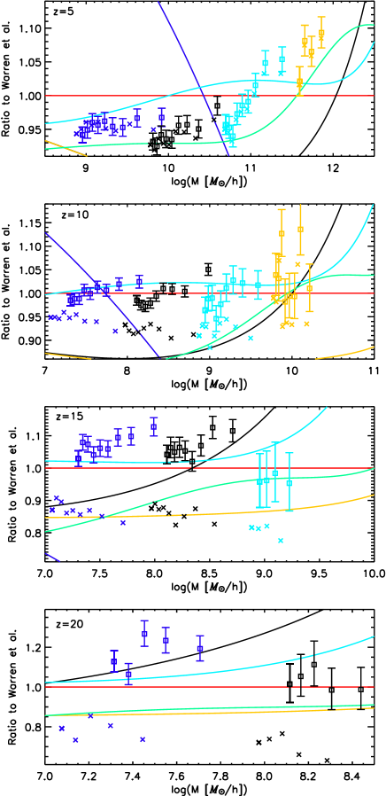
Figure 13:

Mass function corrected for a finite box using the assumption of strict universality, as described in §5.6.1 (squares). Again, we show uncorrected data as well (crosses), and follow the conventions of Fig. 10. This correction produces a clear systematic shift in the results across box boundaries.

For completeness, we mention two other approaches aimed at box-adjusting the mass function. The first (Yoshida et al. 2003c; Bagla & Prasad 2006) simply replaces the original mass variance (eq. (3)) with

$$\sigma^{2}_{\rm box}(M,z)=\frac{d^{2}(z)}{2\pi^{2}}\int^{\infty}_{2\pi/L}k^{2}P(k)W^{2}(k,M)dk\ ,$$ (59)

the lower cut-off arising from imposing periodic boundary conditions ($L$ is the box-size). (For enhanced fidelity with simulations, the integral in eq. [59] goes to a sum over the simulation box modes.) This approach basically assumes that $\sigma$ defined via an infrared cutoff is the appropriate replacement for the infinite-volume mass variance. Figure 13 shows the effect of this suggested correction: At $z=0$ and 5 it is not noticeable, but at higher redshifts the correction is significant relative to the accuracy with which the binned mass function is determined. Furthermore, it exhibits systematic shape changes and offsets across boxes, in contrast to the results shown in Figure 12. For example, at $z=10$ the corrected data at the crossover point between the 4 and 8$\,h^{-1}$Mpc boxes ($\sim 10^{8}\,h^{-1}M_{\odot}$) have an offset of $5\%$. We conclude that this approach is disfavored by our simulation results.

An alternative strategy is to estimate the mass variance from each realization of $P(k)$ in the individual simulation boxes and to treat every box individually, as done in Reed et al. (2007). This has in fact two purposes: to compensate for the realization-to-realization variation in density fluctuations (which could be a problem for small boxes) and also to compensate for an overall suppression in the mass function as discussed above. The disadvantage is that each of many realizations now has a different $\sigma(M)$ for a given value of $M$.

5.7 Mass Function Universality

Finally, we investigate the universality of the mass function found by Jenkins. Approximate universality is expected from the analytic arguments of PS and the extended, excursion-set formulation of Bond et al. (1991). The universal behavior of halo formation persists even in the model of ellipsoidal collapse of ST, in which the predicted mass function is no longer of the PS form. On the other hand, the universality cannot be exact if the nonlinear interactions of different scales are fully accounted for: The nonlinear evolution that leads to the formation of halos of mass $M$ must involve multiple degrees of freedom that are described by more parameters than the overall variance of the primordial overdensity smoothed by a top-hat filter $W(r,M)$. The universality is expected to be violated at sufficiently high resolution of the mass function even in the PS-type spherical collapse model: It is more reasonable to represent the probability of the collapse not by a fraction of particles at the center of spheres enclosing a mass $M$ but by any fraction of particles belonging to such spheres (Betancort-Rijo & Montero-Dorta, 2006a). The improved mass-function derived from this argument deviates somewhat from a universal form (Betancort-Rijo & Montero-Dorta, 2006b).

To investigate the extent our numerical simulations are consistent with universality, we combine our results for $f(\sigma,z)$ as a function of the variance $\sigma^{-1}$ from the entire simulation set in one single curve at various redshifts. This curve is expected to be independent of redshift if universality holds. We display the results in Figure 14 for the raw data and in Figure 15 for the same data after applying the volume corrections discussed earlier.

In the raw data of Figure 14, the agreement with the various fits is quite tight (except for PS) until $\ln\sigma^{-1}>0.3$. Beyond this point, the multiple-redshift simulation results do not lie on top of each other; in the absence of any possible systematic deviation, this would denote a failure of the universality of the FOF, $b=0.2$ mass function at small $\sigma$. Note also that beyond this point the ST and Jenkins fits have a steeply rising asymptotic behavior (relative to the Warren fit). The Reed et al. (2003) fit, meant to be valid over the range $-1.7\leq\ln\sigma^{-1}\leq 0.9$, is in better agreement with our results, to the extent that a single fit can be overlaid on the data.

The ostensible violation of universality seen above is small, however, and subject to a systematic correction due to the finite simulation volume(s). On applying the correction discussed in Section 5.6.3, we obtain the results shown in Figure 15, the key difference being that beyond $\ln\sigma^{-1}>0.3$ the multiple-redshift simulation results now lie on top of each other and, within the statistical resolution of our simulations, are consistent with universal behavior. Specifically, we do not observe the sort of violation reported by Reed et al. (2007) at high redshifts. This could be due to several factors. The finite-sampling FOF mass correction and the finite-volume corrections we employ are different from those of Reed et al. (2007) and the boxes we use at high redshifts are significantly larger. We note also that the difference between the Warren fit and the $z$-dependent fit of Reed et al. (2007) does not appear to be statistically very significant given their data.

6 Conclusions and Discussion

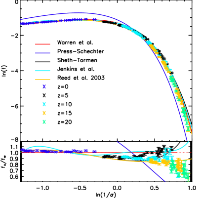
Figure 14: Scaled differential mass function from all simulations, prior to applying finite-volume corrections. Fits shown are Warren (red), PS (dark blue), ST (black), Jenkins (light blue), and Reed et al. (2003) (yellow). Dashed lines denote an extrapolation beyond the original fitting range. The bottom panel shows the ratio relative to the Warren fit. The failure of the different redshift results to lie on top of each other at small values of $\sigma$ indicate a possible violation of universality.

We have investigated the halo mass function from $N$-body simulations over a large mass and redshift range. A suite of 60 overlapping-volume simulations with box sizes ranging from 4 to 256$\,h^{-1}$Mpc allowed us to cover the halo mass range from 10⁷ to 10${}^{13.5}\,h^{-1}M_{\odot}$ and an effective redshift range from $z=0$ to 20.

In order to reconcile conflicting results for the mass function at high redshifts, as well as to investigate the reality of the breakdown of the universality of the mass function, we have studied various sources of error in $N$-body computations of the mass function. A set of error control criteria need to be satisfied in order to obtain accurate mass functions. These simple criteria include an estimate for the necessary starting redshift, for the required mass and force resolution to resolve the halos of interest at a certain mass and redshift, and for the number of time steps.

The criteria for the initial redshift appear to be particularly restrictive. For small boxes, commonly used in the study of the formation of the first objects in the Universe, significantly higher initial redshifts are required than is the normal practice. A violation of this criterion leads to a strong suppression of the mass function, most severe at high redshifts. Recent results by other groups may be contaminated due to a violation of this requirement; a careful re-analysis of small-box simulations is apparently indicated.

The force resolution criterion is especially useful for grid codes, PM as well as adaptive mesh. The mass function can be obtained reliably from PM codes down to small-mass and up to high-mass halos provided the halos are adequately resolved. The resolution criterion is also very useful in setting refinement levels for adaptive mesh refinement (AMR) codes. As shown recently (O’Shea et al. 2005; Heitmann et al. 2005, 2007) the mass function from AMR codes is suppressed at the low-mass end if the base refinement level is too coarse. A more detailed analysis on how to incorporate our results to improve the efficiency of AMR codes is underway.

The results for the required number of time steps to resolve the mass functions is somewhat surprising. The halo mass function appears to be very robust with respect to the number of time steps chosen to follow the evolution, even though the inner structure of the halos will certainly not be correct. Even a small number of time steps is sufficient to obtain a close-to-correct mass function at $z=0$. This considerably simplifies the study of the mass function and its evolution.

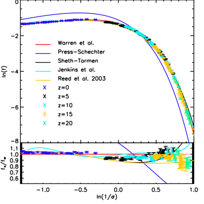
Figure 15: Volume-corrected scaled differential mass function following Fig.14. Note the significantly improved agreement with universal behavior (overlapping results beyond $\ln\sigma^{-1}\sim 0.3$).

Since finite-volume effects can also lead to a suppression of the mass function, we have tried to minimize the importance of these effects by avoiding too-small box sizes, by using overlapping boxes, and by restricting the mass range investigated in a given box size. In addition, we have found that a box-size correction motivated by the extended Press-Schechter formalism for the mass variance appears to give consistent results when applied to our multiple-box simulation ensembles.

We now briefly comment on results found previously by other groups. Jang-Condell & Hernquist (2001) find good agreement with the PS fit at $z=10$ for a mass range $4\times 10^{5}-4\times 10^{8}\,h^{-1}M_{\odot}$. The crossover of PS with the more accurate fits at $z=10$ takes place in exactly this region (see Figs. 1 and 10). Therefore, all fits are very close, and the mass function from a single 1 Mpc box at a single redshift as shown in Jang-Condell & Hernquist (2001) cannot distinguish between them.

As mentioned earlier in §2.5, good agreement with the PS result has been reported at high redshifts (some results being even lower than PS) by several other groups (Yoshida et al. 2003a, 2003b, 2003c; Cen et al. 2004; Trac & Cen 2006). The simulations of Cen et al. (2004) and Trac & Cen (2006) were started at $z_{\rm in}\sim 50$, substantially below the starting redshift that would be suggested by our work. The very large number of particles in the Trac & Cen (2006) simulation requires a high starting redshift (Fig. 5). Therefore, the depressed mass function results of these simulations are very consistent with a too-low initial redshift. (Trac & Cen (2006) have recently rerun their simulations with a much higher initial redshift [$z=300$], and now find results consistent with ours.) The initial particle density of the Iliev et al. (2006) simulations is very close to that of our 16$\,h^{-1}$Mpc box, in which case also a high redshift start is indicated (we used $z_{\rm in}=200$). Finally, the initial redshift of the Yoshida et al. papers, $z_{\rm in}=100$, for boxes of size $\sim 1\,h^{-1}$Mpc, also appears to be significantly on the low side.

We have compared our simulation results for the mass function with various fitting functions commonly used in the literature. The recently introduced ($z=0$) fit of Warren leads to good agreement (at the 20% level with no volume correction, and at the 5% level with volume correction) at all masses and all redshifts we considered. Other modern fits, such as Reed et al. (2003, 2007), also lie within this range. These fits do not suffer from the overprediction of large halos at high redshifts observed for the ST fit. The PS fit performs poorly over almost all the considered mass and redshift ranges, at certain points falling below the simulations by as much as an order of magnitude.

The evolution of the mass function can be used to test the (approximate) universality of the FOF, $b=0.2$ mass function. At low redshifts our data are in good agreement with those of Reed et al. (2007) (at $z=5$), finding a (possible) mild redshift dependence (at the 10% level). At higher redshifts, however, we find that volume corrections are important to the extent that little statistically significant evidence for breakdown of universality remains in our mass function data. A full theoretical understanding of this very interesting result remains to be elucidated.

We have made no attempt to provide a fitting function for our data due to several reasons. First, the current simulation state of the art has not reached the point that one can be confident of percent-level agreement between results from different simulations even in regimes that are not statistics-dominated Heitmann et al. (2007). Second, simulations have not sufficiently explored the extent to which universal forms for the mass function are indeed applicable as cosmological parameters are systematically varied. Third, absent even a compelling phenomenological motivation for the choice of fitting functions, there is an inherent arbitrariness in the entire procedure. Finally, it is not clear how to connect the FOF mass function to observations. In general, tying together mass-observable relations requires close coupling of simulations and observational strategies. In studies of cosmological parameter estimation, we support working directly with simulations rather than with derived quantities, which would add another layer of possible systematic error. Because observations already significantly constrain the parametric range, and are a smooth function of the parameters, this approach is quite viable in practice (Heitmann et al. 2006b; Habib et al. 2007).

.1 Small-Volume Simulations

Small-box simulations of side $\sim 1\,h^{-1}$Mpc have been performed by several groups. Using a treecode with softening length $0.4\,h^{-1}$kpc, and a 1$\,h^{-1}$Mpc box with $128^{3}$ particles, Jang-Condell & Hernquist (2001) evolved their simulation from $z_{\rm in}=100$ to $z=10$. With a halo finder that combined overdensity criteria with an FOF algorithm, the mass function was determined over the range $10^{5.5}-10^{8.1}\,h^{-1}M_{\odot}$, keeping halos with as few as eight particles. At $z=10$ they found “remarkably close agreement” with the PS fit but did not quantify the agreement explicitly.

In a series of papers, Yoshida et al. ran simulations with similar box sizes as above, most including the effects of gas dynamics. The simulations were performed with the TreePM/smoothed particle hydrodynamics code GADGET-II Springel (2005) and followed the evolution of 2$\times$ 324³ particles (324³ in the case of dark matter only), covering a halo mass range of 10⁵-10${}^{7.5}M_{\odot}$. All simulations were started at $z_{\rm in}=100$ from “glass” initial conditions (Baugh et al. 1995; White 1996), in contrast to the grid-based initial conditions used here. The focus of Yoshida et al. (2003a) was the origin of primordial star-forming clouds. As part of that investigation, a dark-matter-only simulation in a 1.6$\,h^{-1}$Mpc box was carried out. The halo density results for $z=20$ to 32 lay systematically below the PS prediction, with the discrepancy being worse at high redshifts. The authors argued that this low abundance of halos was (possibly) due to finite-box-size effects. In Yoshida et al. (2003b), the mass function at $z=20$ for a warm dark matter model was compared with CDM, with the simulation set up being very similar to that of Yoshida et al. (2003a), a 1 Mpc box started at $z=100$. The results obtained were also similar; at $z=20$ the CDM mass function was in good agreement with the PS fit. In a third paper, Yoshida et al. (2003c), a running spectral index was considered. Here results for a standard CDM mass function for a 1 Mpc box were given, this time at $z=17$ and 22. Consistent with their previous results, they found good agreement with PS at these redshifts. (The FOF linking length used in the last paper was $b=0.2$, while in the first two papers $b=0.164$ was chosen. This did not appear to make much of a difference, however.) These papers do not quantitatively compare the numerical mass function to the PS fit. (In contrast to these findings, a recent 1 Mpc box GADGET-II simulation with $z_{\rm in}\sim 120$ has been performed by Maio et al. (2006) who find good agreement with the Warren fit as extrapolated by linear theory – in clear disagreement with PS.)

A similar strategy was followed in Cen et al. (2004) who investigated dark matter halos in a mass range of $10^{6.5}$ to $10^{9}\,h^{-1}M_{\odot}$, using a TreePM code (Xu 1995; Bode et al. 2000). The box size was taken to be $4\,h^{-1}$Mpc, the softening length was set at $0.14\,h^{-1}$kpc, $512^{3}$ particles were used, and the simulations had a starting redshift of $z_{\rm in}=53$. Halos were identified using the overdensity scheme DENMAX Bertschinger & Gelb (1991). Among other quantities, they studied the mass function between $z=11$ and 6 and found that the PS function “provides a good fit” but without explicit quantification.

Overall, these small-box simulations, run with different codes and different halo finders, all found a “depressed” mass function (see Fig. 1), consistent with PS and deviating very significantly from the predictions of the more modern fitting forms. In contrast, other simulations also using small boxes have come to quite different conclusions. For example, in Reed et al. (2007), a large suite of different box sizes and simulations was used to cover the mass range between 10⁵ and 10${}^{11.5}\,h^{-1}M_{\odot}$ at high redshift. The smallest boxes considered in this study were 1 $\,h^{-1}$Mpc on a side. The authors studied the halo mass function at redshifts out to $z=30$, implementing a correction scheme to account for finite-box effects, as discussed in more detail below. Overall, Reed et al. (2007) confirmed previous results as found by Reed et al. (2003) and Heitmann et al. (2006a): PS underestimates the mass function considerably (by at least a factor of 5 at high redshift and high masses), and ST overpredicts the halo abundance at high redshift.

.2 Large-Volume Simulations

The large-box strategy is exemplified by a recent dark matter simulation with the GADGET-II code Springel et al. (2005). The evolution of 2160³ particles in a $500\,h^{-1}$Mpc box was followed from $z_{\rm in}=127$ until $z=0$. The softening length was $5\,h^{-1}$kpc. The high mass and force resolution was sufficient to study the mass function reliably down to a redshift of $z=10$, covering a mass range of $10^{10}$ to $10^{16}\,h^{-1}M_{\odot}$, with halos being identified by a standard FOF algorithm with $b=0.2$. The results are consistent with the Jenkins fit, even though the mass function points at redshifts $z=1.5$, 3.06, and 5.72 are slightly higher than the Jenkins fit and slightly lower for $z=10$. No residuals were shown nor quantitative statements made.

In two recent papers, Iliev et al. (2006) and Zahn et al. (2007) investigated cosmic reionization, providing mass function results at high redshift as part of this work. Iliev et al. (2006) ran a PM simulation with PMFAST (Merz et al. 2005) in a 100$\,h^{-1}$Mpc box with 1624³ particles on a 3248³ mesh. They present results for the mass function at redshifts between $z=6$ and 18.5, using a spherical overdensity halo finder. At lower redshifts they find good agreement with ST, and at high redshift ($z>10$) the results are closer to PS (because of their limited mass range, a more quantitative statement is difficult to make). Zahn et al. (2007) ran a 1024³ particle simulation (dark matter only) in a 65.6$\,h^{-1}$Mpc box with GADGET-II and analyzed the FOF, $b=0.2$ mass function out to $z=20$. Between $z=6$ and 14 they found good agreement with ST in the mass range of 10⁹ to $10^{12}M_{\odot}$. At $z=20$ they found that the simulation results were below ST but above PS, in relatively good agreement with the recent findings of Heitmann et al. (2006a) and Reed et al. (2007).

.3 Medium Volume Simulations

Reed et al. (2003) chose a compromise between the large- and small-box strategies by picking a 50$\,h^{-1}$Mpc box sampled with 432³ particles. The tree code PKDGRAV was used to evolve the simulation from different starting redshifts between $z_{\rm in}=139$ and 69 until $z=0$. The smallest halo contained 75 particles, leading to a mass range of roughly 10¹⁰ to $10^{14.5}\,h^{-1}M_{\odot}$. Good agreement (better than 10%) was found with the ST fit up to $z\simeq 10$. For higher redshifts, the ST fit overpredicted the number of halos, up to 50% at $z=15$. At this high redshift, statistics were lacking, and the resolution was not sufficient to resolve very small halos. A more recent 50$\,h^{-1}$Mpc simulation with PMFAST with $z_{\rm in}=60$ has been carried out by Trac & Cen (2006) using a spherical overdensity definition of halo mass. In this work, the mass function, in the redshift range $6<z<15$, is found to be in very good agreement with PS, in gross contradiction with the results of most of the other simulations mentioned above. (This contradiction has recently been resolved by rerunning their simulation with $z_{in}=300$ and identifying halos with a $b=0.2$ FOF finder.)

References

- Bagla & Prasad (2006) Bagla, J.S. & Prasad, J. 2006, MNRAS, 370, 993
- Barkana & Loeb (2004) Barkana, R. & Loeb, A. 2004, ApJ, 609, 474
- Baugh et al. (1995) Baugh, C.M., Gaztañaga, E., Efstathiou, G. 1995, MNRAS, 274, 1049
- Bertschinger & Gelb (1991) Bertschinger, E. & Gelb, J.M. 1991, Computers in Physics, 5, 164
- Betancort-Rijo & Montero-Dorta (2006a) Betancort-Rijo, J.E. & Montero-Dorta, A.D. 2006, ApJ, 650, L95
- Betancort-Rijo & Montero-Dorta (2006b) Betancort-Rijo, J.E. & Montero-Dorta, A.D. 2006, ApJ, 653, L77
- Bode et al. (2000) Bode, P., Ostriker, J.P., & Xu, G.H. 2000, ApJS, 128, 561
- Bond et al. (1991) Bond, J.R., Cole, S., Efstathiou, G., & Kaiser, N. 1991, ApJ 379, 440
- Bowman et al. (2006) Bowman, J.D., Morales, M.F., & Hewitt, J.N. 2006, ApJ, 638, 20
- Bunn & White (1997) Bunn, E.F. & White, M. 1997, ApJ, 480, 6
- Cen et al. (2004) Cen, R., Dong, F., Bode, P., & Ostriker, J.P. 2004, astro-ph/0403352
- Crocce et al. (2006) Crocce, M., Pueblas, S. & Scoccimarro, R. 2006, MNRAS, 373, 369
- Davis et al. (1985) Davis, M., Efstathiou, G., Frenk, C.S. 1985, ApJ, 292, 371
- Einasto et al. (1984) Einasto, J., Klypin, A.A., Saar, E., Shandarin, S.F. 1984, MNRAS, 206, 529
- Evrard (2004) Evrard, A.E. 2004, in Clusters of Galaxies: Probes of Cosmological Structure and Galaxy Evolution, edited by J.S. Mulchaey, A. Dressler, & A. Oemler (Cambridge: Cambridge Univ. Press), 1
- Evrard et al. (2007) Evrard, A.E. et al. 2007, in press (astro-ph/0702241)
- Furlanetto et al. (2006) Furlanetto, S.R., McQuinn, & M., Hernquist, L., 2006, MNRAS, 365, 115
- Gelb & Bertschinger (1994) Gelb, J.M. & Bertschinger, E. 1994, ApJ, 436, 467
- Habib et al. (2007) Habib, S., Heitmann, K., Higdon, D., Nakhleh, C., & Williams, B., 2007, Phys. Rev. D, 76, 083503
- Haiman & Loeb (2001) Haiman Z. & Loeb A. 2001, ApJ, 552, 459
- Heinrich (2003) Heinrich, J. 2003, Coverage of Error Bars for Poisson Data (CDF Note 6438; Batavia: Fermilab)
- Heitmann et al. (2007) Heitmann, K., Lukić, Z., Fasel, P., Habib, S., Warren, M.S., White, M., Ahrens, J., Ankeny, L., Armstrong, R., O’Shea, B., Ricker, P.M., Springel, V., Stadel, J., and Trac, H., 2007, preprint, astro-ph/0706.1270
- Heitmann et al. (2006a) Heitmann, K., Lukić, Z., Habib, S., & Ricker, P.M. 2006, ApJ, 642, L85
- Heitmann et al. (2006b) Heitmann, K., Higdon, D., Nakhleh, C., & Habib, S., 2006, ApJ, 646, L1
- Heitmann et al. (2005) Heitmann, K., Ricker, P.M., Warren, M.S., & Habib, S. 2005, ApJS, 160, 28
- Holder et al. (2001) Holder, G., Haiman Z., & Mohr, J. 2001, ApJ, 560, L111
- Hu & Sugiyama (1996) Hu, W. & Sugiyama, N. 1996, ApJ 471, 542
- Iliev et al. (2006) Iliev, I.T., Mellema, G., Pen, U.-L., Merz, H. Shaprio, P.R., & Alvarez, M.A. 2006, MNRAS, 369, 1625
- Jang-Condell & Hernquist (2001) Jang-Condell, H. & Hernquist, L. 2001, ApJ, 548, 68
- Jenkins et al. (2001) Jenkins, A. et al. 2001, MNRAS 321, 372 (JENKINS)
- Katz et al. (1993) Katz, N., Quinn, T., & Gelb, J.M. 1993, MNRAS, 265, 689
- Lacey & Cole (1993) Lacey, C.G. & Cole, S. 1993, MNRAS, 262, 627
- Lee & Shandarin (1998) Lee, J. & Shandarin, S. 1998, ApJ, 500, 14
- Le Fevre et al. (2005) Le Fevre, O., Paltani, S., Arnouts, S., Charlot, S., Foucaud, S., Ilbert, O., McCracken, H.J., Zamorani, G., the VIMOS VLT Deep Survey team 2005, Nature, 437, 519
- Maio et al. (2006) Maio, U. et al. 2006, MNRAS, 373, 869
- MacTavish et al. (2006) MacTavish, C.J. et al. 2006, ApJ, 647, 799
- Merz, Pen, & Trac (2005) Merz, H., Pen, U.L., & Trac, H. 2005, New Astron., 10, 393
- Mo & White (1996) Mo, H.J. & White, S.D.M. 1996 MNRAS, 282, 347
- Mobasher et al. (2005) Mobasher, B. et al. 2005, ApJ, 635, 832
- Naoz & Barkana (2007) Naoz, S. & Barkana, R. 2007, MNRAS, 377, 667
- Navarro et al. (1997) Navarro, J.F., Frenk, S.C., & White, S.D.M. 1997, ApJ, 490, 493
- O’Shea et al. (2005) O’Shea, B.W., Nagamine, K., Springel, V., Hernquist L., & Norman, M.L. 2005, ApJS, 160, 1
- Peebles (1980) Peebles, P.J.E. 1980, The Large-Scale Structure of the Universe (Princeton: Princeton Univ. Press)
- Press & Schechter (1974) Press, W.H. & Schechter, P. 1974, ApJ, 187, 425 (PS)
- Reed et al. (2003) Reed, D. et al. 2003, MNRAS, 346, 565
- Reed et al. (2005) Reed, D. et al. 2005, MNRAS, 363, 393
- Reed et al. (2007) Reed, D., Bower, R., Frenk, C., Jenkins, A. and Theuns T. 2007, MNRAS, 374, 2
- Seljak & Zaldarriaga (1996) Seljak, U. & Zaldarriga, M. 1996, ApJ, 469, 437
- Sheth & Tormen (1999) Sheth, R.K. & Tormen, G. 1999, MNRAS, 308, 119 (ST)
- Sheth & Tormen (2002) Sheth, R.K. & Tormen, G. 2002, MNRAS, 329, 61
- Sheth et al. (2001) Sheth, R.K., Mo, H.J., & Tormen, G. 2001, MNRAS, 323, 1
- Spergel et al. (2007) Spergel, D.N., 2007, ApJS, 170, 377
- Springel (2005) Springel, V. 2005, MNRAS, 364, 1105
- Springel et al. (2005) Springel, V. et al. 2005, Nature, 435, 629
- Summers et al. (1995) Summers, F.J., Davis, M. & Evrard, A.E. 1995, ApJ, 454, 1
- Tegmark et al. (1997) Tegmark, M. et al. 1997, ApJ, 474, 1
- Trac & Cen (2006) Trac, H. & Cen, R. 2006, preprint astro-ph/0612406
- Valageas (2002) Valageas, P. A&A 2002, 385, 761
- Voit (2005) Voit, G.M. 2005, Rev. Mod. Phys., 77, 207
- Warren et al. (2006) Warren, M.S., Abazajian, K., Holz, D.E., & Teodoro, L. 2006, ApJ, 646, 881 (Warren)
- White (2001) White, M. 2001, AA, 367, 27
- White (2002) White, M. 2002, ApJS, 143, 241
- White (1996) White, S.D.M. 1996, in Cosmology and Large-Scale Structure, ed. R. Schaefer et al. (Amsterdam: Elsevier), 349
- Xu (1995) Xu, G. 1995, ApJS, 98, 355
- Yoshida et al. (2003a) Yoshida, N., Abel, T., Hernquist, L., & Sugiyama, N. 2003, ApJ, 592, 645
- Yoshida et al. (2003b) Yoshida, N., Sokasian, A., Hernquist, L., & Springel, V. 2003, ApJ, 591, L1
- Yoshida et al. (2003c) Yoshida, N., Sokasian, A., Hernquist, L., & Springel, V. 2003, ApJ, 598, 73
- Yoshida et al. (2003) Yoshida, N., Sugiyama, N., & Hernquist, L. 2003, MNRAS, 344, 481
- Zahn et al. (2007) Zahn, O., Lidz, A., McQuinn, M., Dutta, S., Hernquist, L., Zaldarriaga, M., & Furlanetto, S.R. 2007, ApJ, 654, 12
- Zel’dovich (1970) Zel’dovich, Y.B. 1970, A& A, 5, 84