The dynamics of tidal tails from massive satellites

Abstract

We investigate the dynamical mechanisms responsible for producing tidal tails from dwarf satellites using N-body simulations. We describe the essential dynamical mechanisms and morphological consequences of tail production in satellites with masses greater than 0.0001 of the host halo virial mass. We identify two important dynamical co-conspirators: 1) the points where the attractive force of the host halo and satellite are balanced (X-points) do not occur at equal distances from the satellite centre or at the same equipotential value for massive satellites, breaking the morphological symmetry of the leading and trailing tails; and 2) the escaped ejecta in the leading (trailing) tail continues to be decelerated (accelerated) by the satellite’s gravity leading to large offsets of the ejecta orbits from the satellite orbit. The effect of the satellite’s self gravity decreases only weakly with a decreasing ratio of satellite mass to host halo mass, proportional to $(M_{s}/M_{h})^{1/3}$, demonstrating the importance of these effects over a wide range of subhalo masses. Not only will the morphology of the leading and trailing tails for massive satellites be different, but the observed radial velocities of the tails will be displaced from that of the satellite orbit; both the displacement and the maximum radial velocity is proportional to satellite mass. If the tails are assumed to follow the progenitor satellite orbits, the tails from satellites with masses greater than 0.0001 of the host halo virial mass in a spherical halo will appear to indicate a flattened halo. Therefore, a constraint on the Milky Way halo shape using tidal streams requires mass-dependent modelling. Similarly, we compute the the distribution of tail orbits both in $E_{r}-r^{-2}$ space (Lynden-Bell & Lynden-Bell 1995) and in $E-L_{z}$ space (Helmi & de Zeeuw 2000), advocated for identifying satellite stream relics. The acceleration of ejecta by a massive satellite during escape spreads the velocity distribution and obscures the signature of a well-defined “moving group” in phase space. Although these findings complicate the interpretation of stellar streams and moving groups, the intrinsic mass dependence provides additional leverage on both halo and progenitor satellite properties.

1 Introduction

According to the currently favoured galaxy formation scenario, the cold dark matter (CDM) cosmogony, galaxies are built up from the assembly of small structures. In this paradigm the assembly mechanism plays a key role in understanding the formation history of galaxies. Recent cold dark matter cosmological numerical simulations predict the existence of a large population of subhalos. Comparisons with the observed population of dwarf galaxies and detailed predictions of the present-day subhalo population, dark or luminous, have become important tests of the CDM galaxy formation paradigm (Ghigna et al., 1998, 2000; De Lucia et al., 2004; Diemand et al., 2004; Gao et al., 2004; Oguri & Lee, 2004). Most studies to date use large cosmological simulations and classify their properties statistically. However, to properly investigate these processes, one needs to perform high resolution idealised simulations of subhalo evolution within the CDM paradigm (Hayashi et al., 2003). Alternatively, in this study, we investigate one important consequence of subhalo disruption: the formation and evolution of tidal tails. By adopting initial conditions motivated by the CDM simulations, we can focus our computational resources on understanding the dynamical mechanism.

Satellite galaxy tidal tails are an important observable fossil signature to help understand the formation history of the Milky Way and to test CDM theory as a consequence. Tails and streams provide information about the Galactic halo mass model as well as the evolutionary history of the observed satellite galaxy. In the CDM model, galaxies are embedded in massive dark matter halos. Estimating dark matter halo structure is essential to understand galaxy formation and tidal tail morphology probes halo structure (Johnston et al., 1999; Helmi & de Zeeuw, 2000; Ibata et al., 2001a, b). Several space missions, for example the ESA astrometric satellite GAIA (Lindegren & Perryman, 1996; Perryman et al., 2001), are planned to measure the position and motion of stars in the Milky Way with very high accuracy, in the near future. Together with ground-based radial velocity experiments, e.g. RAVE (Steinmetz et al., 2006), these surveys will provide full phase space information. Accurate six dimensional phase space information of Milky Way stars will provide observational information of the tidal tail and hence the formation history of the Milky Way. The time is ripe to carry out a detailed theoretical study of satellite galaxy disruption and the induced tidal tail morphology.

In this study we perform numerical simulations of satellite galaxy disruption and its induced tidal tail morphology within the CDM cosmogony. The objective of this study is to understand the physical processes responsible for satellite galaxy disruption rather than reproducing the evolutionary history of any individual Milky Way satellite galaxy. In particular, satellite disruption in N-body simulations is produced by escaping satellite particles. In addition, the gravitational shock, which is caused by the slowly varying host halo potential as the satellite goes through its orbit, changes the satellite’s internal structure. An initially stable satellite galaxy and accurate numerical integration of a satellite particle’s orbit are necessary to represent these physical processes correctly. We investigate satellite galaxy evolution by performing high resolution and low noise N-body simulations with such stable initial conditions.

In addition, we can estimate any trends of satellite tidal tail morphology with satellite properties from our simulations, even though we do not reproduce the evolutionary history of any specific Milky Way satellite. Our simulation results show that the gravity of the satellite alters the location of the tidal tails relative to the satellite orbit. The satellite decelerates (accelerates) the leading (trailing) tail beyond the tidal radius, which is proportional to the satellite mass. For more massive satellites, this results in the leading tail being located well inside and the trailing tail being located well outside of the satellites orbit, rather than tracking the original satellite orbit (Johnston et al., 1996, 2001; Moore & Davis, 1994). Since the satellite torques the tidal tail, the distribution of the tidal tail in the observational plane is rather different from predictions that exclude such satellite torquing. In addition, the simulations provide six-dimensional phase-space information of the tidal tail to compare with upcoming astrometric measurements.

In Section, 2 we describe how we make stable satellite initial conditions and provide a brief overview of the simulation algorithm. In Section, 3 we investigate satellite disruption and the formation of the tidal tail, including the effects of the satellite potential on the tidal tail, and in Section 4, we investigate the observational consequences. In Section 5, we summarise our results and discuss their importance.

2 Initial conditions and N-body methodology

Table 1: Initial properties of the three satellite models

Satellite	$M/M_{vir,host}$	$R/R_{vir,host}$	$V_{max}/V_{max,host}$
Massive	$1.9\times 10^{-2}$	$9.02\times 10^{-2}$	0.45
Low-Mass	$9.0\times 10^{-4}$	$3.38\times 10^{-2}$	0.16
Tiny-Mass	$9.9\times 10^{-5}$	$1.66\times 10^{-2}$	0.08

The initial conditions of our simulations are motivated by the CDM cosmology. CDM cosmological simulations suggest that dark matter halos have a universal density profile (Navarro et al., 1997, hereafter NFW), $\rho(r)\propto r^{-1}(r+r_{s})^{-2}$, where $r_{s}$ is a scale length characterised by the concentration parameter $c=R_{vir}/r_{s}$ and $R_{vir}$ is the virial radius of the halo. Although there are some disagreements regarding the accuracy of this simple formula in describing halos in numerical simulations and in comparisons with observed galaxies, it remains the accepted CDM halo density profile and we adopt it for our study.

We represent the host halo by a static NFW halo potential. Hence our simulations ignore the effects of dynamical friction and the subsequent reaction of the host halo. Obviously this is not realistic but since the satellite masses of interest are often much smaller than the host halo mass, the consequences are minor. Moreover, the prime motivation of this study is to understand the physical processes responsible for satellite disruption and tidal tail formation and not the evolutionary history of the satellite. Dynamical friction is not vital to understand these processes.

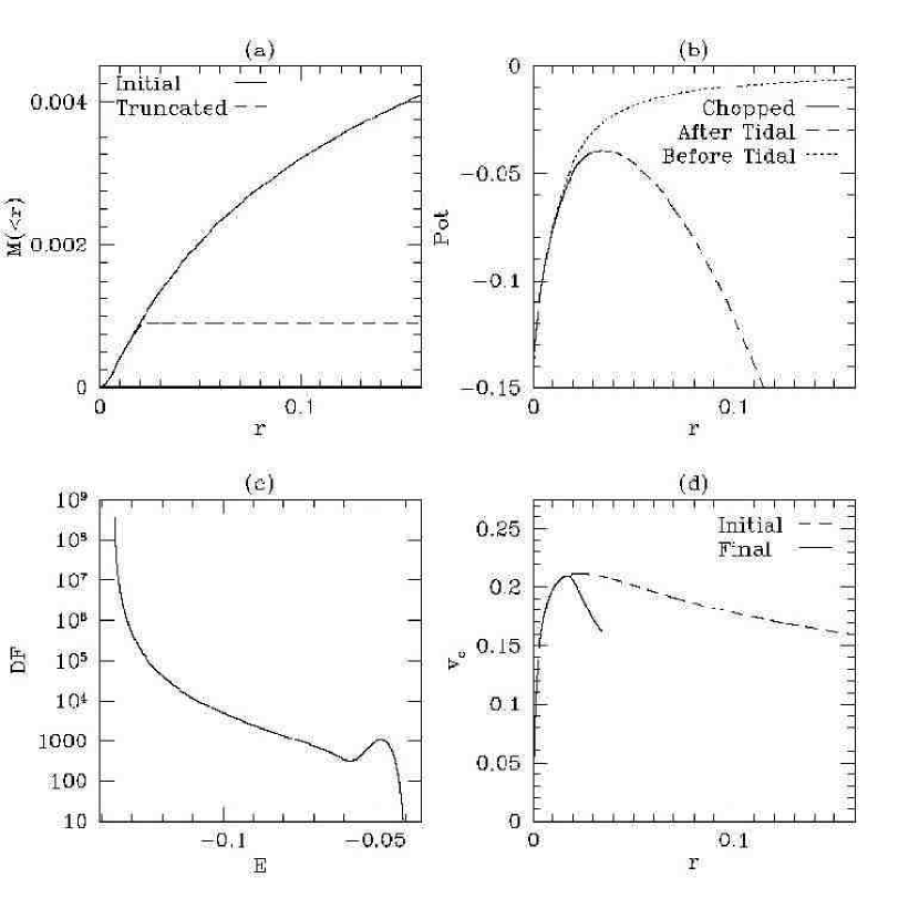
Figure 1: The effect of our truncation procedure (see text) on a satellite’s initial NFW profile. (a) The enclosed mass profile. (b) The effective potential profile. (c) The Distribution function versus energy. (d) The circular velocity profile. We use system units unless otherwise specified: $G=1$, $M_{vir,host}=1$, and $R_{vir,host}=1$.

Before tidal truncation, the satellites have an NFW density profile. However, the NFW profile extends to infinity and real astronomical systems have a finite size. The conventional solution limits the size of an isolated dark matter halo to its virial radius (Gunn & Gott, 1972; Bryan & Norman, 1998). The host halo’s tidal field then determines the size of satellite halo. The host halo’s tidal field affects a satellite halo even before the satellite halo passes within the host halo’s virial radius. As a result, it is computationally expensive to simulate the entire evolution of a satellite. Remember, the objective of our study is to understand the physical processes responsible for tidal tail formation not the reproduction of a particular tail feature. Therefore, we place the satellite in the host halo on the desired orbit to start and include the host halo’s tidal field when we generate a satellite’s initial phase-space distribution. It is natural to characterise the tidal length scale in the satellite by the radius of the X-point that this satellite would have at some fiducial galactocentric radius in its orbit. We call this fiducial radius the tidal distance. In other words, the satellite on a circular orbit at the tidal distance would have the X-point $r_{\times}$. At this point, the gravitational force from the satellite exactly balances the gravitational force from the host halo and non-inertial centrifugal force.

The details of the iterative procedure that we use to generate the satellite’s initial condition is as follows. First, we truncate the virial radius limited NFW satellite halo at the X-point radius, $r_{\times}$, using the error function, $\{1-\hbox{erf}[(r-r_{\times})/s]\}$. We then compute the distribution function using Eddington inversion and calculate a new satellite density profile by integrating the distribution function over velocity. The parameter $s$ in the error function truncation formula is increased from zero until a smooth phase-distribution function results. We iterate these steps until the density–distribution-function pair is converged. Figure 1 shows an example of how this procedure modifies an initial satellite halo. At the conclusion of the procedure, the effective tidal radius is approximately 75% of the initial X-point radius radius. We characterise a satellite halo by its initial maximum circular velocity; Figure 1 demonstrates that this velocity is only weakly affected by the truncation procedure. We denote the outer radius of the satellite after the truncation procedure as the effective tidal radius. It is smaller than $r_{\times}$ owing to the truncation with the error function and the Eddington inversion process. Finally, we use an acceptance-rejection algorithm to generate each particle halo realization. The satellite is made up $10^{6}$ particles. Since the initial satellites are already truncated, satellite particles are ejected only through interactions with the host halo during the simulation.

We simulate a set of satellite realizations with the same tidal distance but different initial maximum rotation velocities. We investigate the effects of a satellite’s size and orbit on its tidal tail morphology by varying them separately but keeping the other parameters fixed. In detail, we choose a $c=15$ NFW model for both the host halo potential and for the satellites. We generate three different size satellites, which we refer to as the massive satellite, the low-mass satellite, and the tiny-mass satellite. We use the maximum rotation velocity, $V_{max,sat}$, as a measure of satellite size since the continuous mass loss makes mass an inexact measure. We use a $V_{max,sat}$ of 0.45, 0.16, and 0.08 times $V_{max,host}$ for the massive, low-mass, and tiny satellite, respectively. The tidal distance for all three satellites is $0.4R_{vir}$. We also set the galactocentric orbital radius to $0.4R_{vir}$ for our circular orbit simulations. After our truncation procedure is complete, the initial mass of the massive satellite is 0.018 $M_{host}$, the low-mass satellite 0.001 $M_{host}$, and the tiny-mass satellite 0.0001 $M_{host}$. Converting our simulation units to a Milky Way size galaxy system and evolving for a few satellite orbits, the low-mass satellite roughly corresponds in mass to the Sagittarius dwarf galaxy halo (Majewski et al., 2004; Law et al., 2005). The massive and tiny-mass satellites are an order of magnitude more and less massive, respectively. The properties of these satellite halos is summarised in Table 1 in units of the virial quantities of the host halo. All satellite initial conditions in this study have $10^{6}$ particles.

We evolve each of the three satellites on three different orbits with the same energy but with different eccentricities. We define the eccentricity of the orbits as $e\equiv(r_{a}-r_{p})/(r_{a}+r_{p})$ where $r_{a}$ and $r_{p}$ are the apocentre and the pericentre of a satellite. The first orbit is circular ($e=0$) at $0.4R_{vir}$. The second orbit has an $e=0.5$ with a pericentre of $0.2R_{vir}$ and an apocentre of $0.6R_{vir}$, and the third orbit has $e=0.74$ with a pericentre of $0.1R_{vir}$ and an apocentre of $0.67R_{vir}$. The third orbit is particularly relevant cosmologically since its circularity ($\kappa$) is 0.5, which is the median $\kappa$ of subhalos in a sample taken from recent cosmological simulations (Ghigna et al., 1998; Zentner et al., 2005). We quote results using the following system units unless otherwise specified: $G=1$, $M_{vir,host}=1$, and $R_{vir,host}=1$. The timestep for our N-body simulations is $2.5\times 10^{-4}$ system time units. Therefore, one circular orbit is made of about $8000$ timesteps because one circular orbit period is $T_{period}\sim 2.0$

Figure 2: Comparison of the evolved density profiles of two identical, low mass satellite halos evolved with different starting radii. The inner orbit begins with $r=0.67R_{vir}$ and a tidal distance corresponding to $0.4R_{vir}$ with an eccentricity $e=0.73$. The virial radius orbit begins with $r=1.0R_{vir}$ and a tidal distance corresponding to $1.0R_{vir}$ with $e=0.5$. Owing to gravitational heating, the evolution of the two satellites is different but the profiles approximately agree when the total mass lose is the same.

Our satellite subhalo is initially truncated without considering its evolutionary history and without including any gravitational heating. This is crudely consistent with our initial condition generation procedure that assumes an equilibrium configuration at some radius inside the host halo to start. Fortunately, this idealised setup does not produce an unrealistic satellite mass loss history. Stoehr et al. (2002) and Hayashi et al. (2003) performed a quantitative study of NFW subhalo evolution in a host halo using idealised N-body simulations and claim that satellites on two different orbits have similar mass and velocity profiles after losing the same amount of mass. To check this, we compared the evolved density profiles of two low-mass satellites on orbits with $e=0.74$ but at two different tidal distances: 1) the radius of a circular orbit with the same energy; and 2) the host halo virial radius, $R_{vir}$. The first test describes the satellite evolution scenario adopted for this study. The second test describes the cosmologically-motivated scenario of a satellite entering the host halo for the first time. Certainly, these two satellites have quite different evolutionary histories. However, when the bound mass of the two satellites is scaled to the same value, their evolved density profiles are similar, as shown in Figure 2. This test, together with the results of Stoehr et al. (2002) and Hayashi et al. (2003), suggests that our tidally truncated satellite models are a fair representation of CDM subhalos (see Figure 10 in Hayashi et al., 2003). In addition, although tidal heating, which is sensitive to a satellite’s structure, plays an important role in the satellite disruption process, we will show that the tidal tail morphology does not depend on a satellite’s inner structure but only on a satellite’s mass and orbit.

For the gravitational potential solver, we use a three-dimensional self-consistent field algorithm (SCF, also known as an expansion algorithm, e.g., Clutton-Brock, 1972, 1973; Hernquist & Ostriker, 1992; Weinberg, 1999). This algorithm produces a bi-orthogonal basis set of density-potential pairs from which it computes the gravitational potential of a N-body system, given the mass and positions of the particles. For an arbitrary basis, e.g. spherical Bessel functions, the expansion generally requires a large number of terms to achieve convergence, which introduces small-scale noise as well as requiring greater computational expense. The situation was dramatically improved by Weinberg (1999) using a numerical solution of the Sturm-Liouville equation to match the lowest-order pair to the equilibrium profile, and therefore, the expansion series converges rapidly. Here, we use the current density profile as the zero-order basis function.

For our purposes, this expansion algorithm is attractive for two reasons. First, the expansions can be chosen to follow structure over an interesting range of scales and simultaneously suppresses small-scale noise. In contrast, noise from two-body scattering can arise at all scales in direct-summation, tree algorithm, and mesh based codes. Small-scale scattering can give rise to a diffusion in conserved quantities, which can lead to unphysical outcomes particularly for studies of long-term galaxy evolution (see Weinberg & Katz, 2007a, b). Second, the expansion algorithm is computationally efficient; the computational time only increases linearly with particle number. Hence, the expansion algorithm permits the use of a much larger number of particles than most other algorithms for the same computational cost.

An accurate potential solver for a cuspy halo demands a precise determination of the expansion centre, ${\bf C}$. This is the major disadvantage of the expansion algorithm relative to a Lagrangian potential solver such as a tree code. We developed and tested the following algorithm for evolving cuspy dark matter halos with an expansion code:

1. At time step $n$, we compute ${\bf C}_{n}$ from the centre of mass of the $N_{min}$ most bound particles;

2. To evaluate the expansion centre at time step $n+1$, a predicted centre ${\bf C}_{pred,n+1}$ is estimated from a linear least squares solution using the previous $N_{keep}$ centres: $\{{\bf C}_{j}|n-N_{keep}<j\leq n\}$;

3. For $n<2$, we set ${\bf C}_{pred,n+1}={\bf C}_{n}$.

4. To reduce truncation error, we separately track the motion relative to the satellite’s centre and the motion of the centre itself.

The linear least squares estimator for the expansion centre ${\bf C}_{pred}$ reduces the Poisson noise from the $N_{min}$ particles used to determine each of the ${\bf C}_{n}$. For our simulations we have adopted $N_{min}=512$ and $N_{keep}=10$ and have verified that this centring scheme maintains the cusp while the satellite orbits in a host halo for situations where the tidal field is insignificant.

3 The morphology of satellite tidal tails

Time-dependent forcing by the host halo’s tidal field adds energy to the satellite, driving mass loss and, ultimately, disruption. These forces are a combination of the differential force from the host halo and the non-inertial forces from the satellite orbit. The work done against the satellite’s gravitational potential results in mass loss. In addition, these forces deform the outer density contours of the satellite. To understand the evolution of the ejecta, one must also consider the gravitational field of the satellite. The gravitational force from the satellite decelerates (accelerates) the leading (trailing) tail, modifying the energy and angular momentum of the ejecta well past the point of escape. The conserved quantities of the ejecta, then, may be dramatically different than that of the satellite centre of mass. The strength of the satellite gravity increases with satellite mass, of course. These effects combine to make the morphology of tidal tails more complicated than previously suggested (Moore & Davis, 1994; Ibata & Lewis, 1998; Johnston et al., 2001; Helmi & White, 1999; Mayer et al., 2002), especially for a massive satellite. We investigate the causes of these effects and their consequences in detail below.

3.1 Satellite disruption

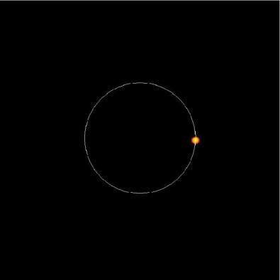
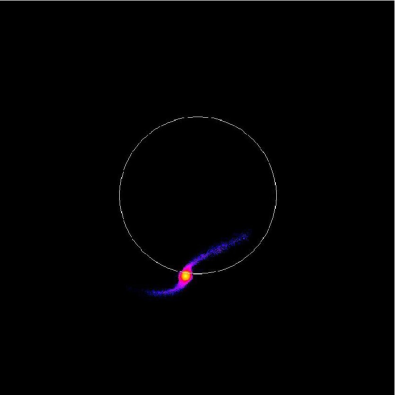
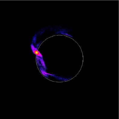
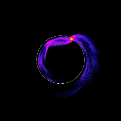
Figure 3: The mass density of the low-mass satellite on a circular orbit with $r=0.4R_{vir}$ at $T=0.0$ (top-left), $1.5$ (top-right), $3.0$ (bottom-left), and $4.5$ (bottom-right). Recall that the orbital period for the circular orbit in this simulation is $T_{period}\approx 2.0$. The colour scale is logarithmic in the dark matter mass density, increasing from blue to red, and is fixed for all times $T$. Each panel has a linear size of 2 host-halo virial radii. For this simulation, the tail particles do not feel the gravitational force of the satellite after escape. The circles show the satellite orbit. The multiple streams in the tail owe to phase crowding near apocentre for initially prograde and retrograde orbits.

We begin by describing the dynamics and morphology of the tidal tails in a simulation that ignores the gravitational field of the satellite past the tidal radius. Figure 3 shows a sequence of snapshots of the low-mass satellite ($0.001M_{host}$) on a circular orbit at $0.4R_{vir}$. We use units where $M_{vir}=1$, $R_{vir}=1$, and Newton’s gravitational constant $G=1$, together which defines a natural time unit. Scaled to the Milky Way, 0.5 natural time units is approximately 1 Gyr. Appealing to the standard zero-velocity Roche potential, which balances the effective gravitational potential in the rotating frame with the halo potential, we expect the mass to become unbound in the vicinity of the Lagrange or X-points. Indeed, we observe the double cometary appearance of tails leading and trailing the satellite, enforced by the conservation of angular momentum. For this halo model, the leading ejecta orbits faster than the satellite and has a position angle of $300^{\circ}$ measured from the positive vertical axis, the direction of satellite’s instantaneous motion. The trailing tail moves slower than the satellite and has a position angle of $120^{\circ}$. Since the simulation in Figure 3 ignores the satellite’s gravity beyond the tidal radius, the orbit of the tidal tail merely represents the kinematic condition of the tail material just when it escapes from the satellite.

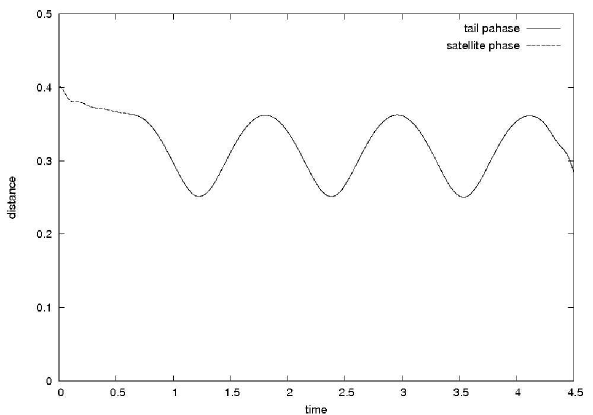
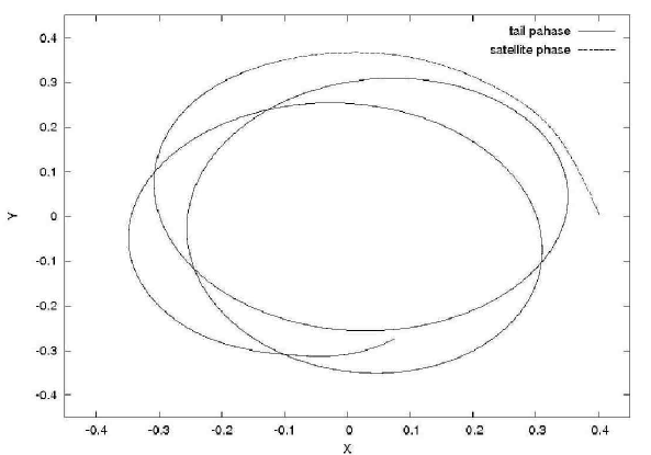
Figure 4: The orbit of a random particle in the leading tail for the simulation presented in Figure 3. The top panel plots galactocentric radius versus time and the bottom panel shows the trajectory in the orbital plane. In both panels, the trajectory is plotted as a dashed line when it is still bound to the satellite and as a solid line after escape. The particle describes a rosette with its apocentre near the satellite orbital radius after escape.

An example of a randomly chosen orbit in the leading tail is shown in Figure 4. As expected, the orbit describes a rosette with its apocentre at the radius of the satellite orbit. The energy and angular momentum lost during the escape changes the conserved quantities of the ejecta orbits from that of the satellite orbit; the leading (trailing) ejecta lose (gain) energy during deformation. Moreover, the distribution of the tails fills a wide region about the satellite orbit. This reflects the broad distribution of phases for orbits at escape. Hence, the width of the tail is nearly the same as the distance between the apocentre and the pericentre of a typical rosette orbit. Each tail has several distinct streamers filling a common envelope. The two primary streams in each tail demarcate the escape of the most extreme prograde and retrograde orbits. The originally prograde orbits have lower specific angular momentum and, therefore, smaller pericentres and larger epicyclic amplitudes. In contrast, originally retrograde orbits have larger pericentres and smaller epicyclic amplitudes. Distinct streamers result from the phase caustics near apocentre, similar to shells in elliptical galaxies caused by merger ejecta with a velocity dispersion much smaller than its new orbital velocity. This mechanism, illustrated in Figure 3, is the massless description of tail formation. This massless description assumes that the orbital energy and angular momentum of a tail is the same as those of a satellite; this yields a simple easy-to-compute prescription for the tails’ location.

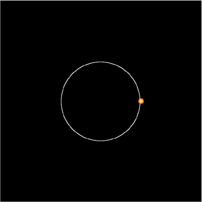
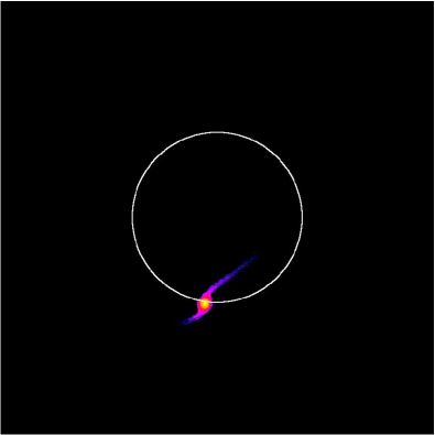
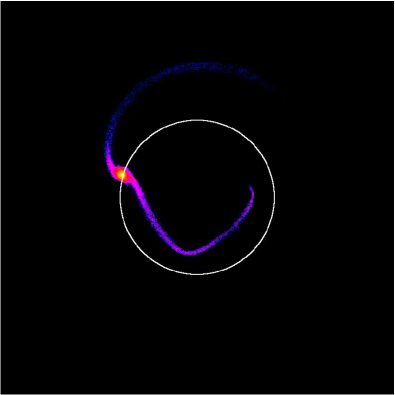
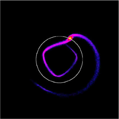
Figure 5: As in Figure 3 but including the gravitational attraction of the satellite on the ejecta at all times.

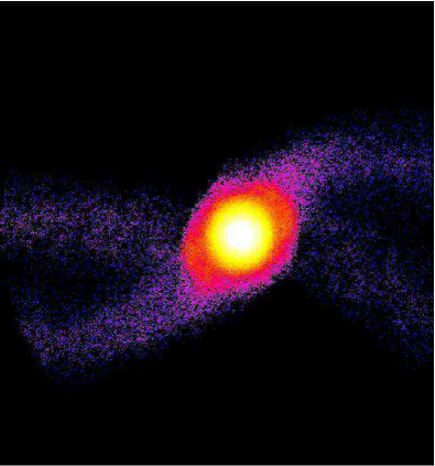
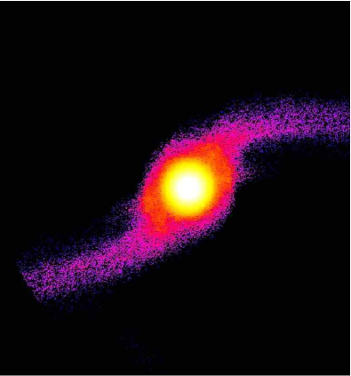
Figure 6: A high-resolution view of the tail streamers in the low-mass satellite simulation without (left) and with (right) the gravitational acceleration by the satellite at $T=4.5$ (compare with Figure 3 left panel, and Figure 5 middle panel, respectively). The two steamers are clear in left panel but very weak in the right panel. Although very weak, the second streamers can be identified near the tidal radius.

In contrast, Figure 5 repeats the simulation including the gravity of both the halo and the satellite at all times. At early times (upper-right panel), the evolution is similar. However, at later times (lower panels), the effects of the satellite gravity are marked. The continued acceleration of the tail by the satellite after escape decreases the internal velocity dispersion and narrows or focuses the tail as a consequence. The streamers in Figure 3 become less distinct when accelerated by the gravity of the satellite and the host halo together for the same reason (see Figure 6). Similarly, the acceleration of the ejecta by the satellite also decreases the angular separation between the streamers. Although the multi-streamer feature is diminished as the satellite gravitational field accelerates the ejecta, the feature can still be seen very close to the tidal radius.

3.2 Tail evolution

3.2.1 Circular orbits

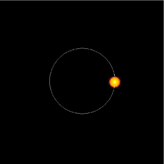
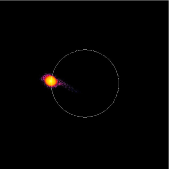
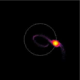
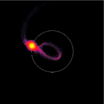
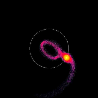
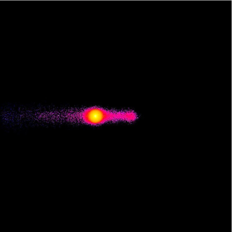
Figure 7: The mass density in the orbital plane for a massive satellite halo on a circular orbit with $r=0.4R_{vir}$ at $T=0.0$, $1.0$, $2.0$, $3.0$, and $4.0$ in the top-left, top-right, middle-left, middle-right, and bottom-left panels, respectively. Recall that the orbital period of the circular orbit is $T_{period}\sim 2.0$. The bottom-right panel shows the edge on view at $T=4.0$. The colour scale is logarithmic in the dark matter mass density from blue to red. The colour scale is fixed for all snapshots (as described in Figure 3). The circles show the satellite orbit. The tail remains confined to the orbital plane as expected (lower-right panel).

The importance of a satellite’s gravity increases with mass and, therefore, we begin with a study of the tail produced by a massive satellite. Figure 7 shows snapshots of a massive satellite ($0.018M_{host}$) on an circular orbit at $0.4R_{vir}$, where once again the tail particles always feel the gravitational force from the satellite. The overall evolution of the satellite and its disruption time is similar to the less massive satellite shown in Figure 5. However, the long-term acceleration of the ejected material by the remaining satellite significantly alters these orbits. As the tail continues to lose mass, the leading and trailing tails evolve to positions that are well inside and well outside the satellite’s orbit and hence does not trace the satellite orbit at all (Johnston et al., 2001; Moore & Davis, 1994). The leading tail significantly tilts toward the centre of the halo and almost points directly there at late times. The trailing tail is distributed throughout a wide annulus in the outer halo. This difference results from the torque applied by the satellite well after escape. Orbits in the leading tail that lose energy and angular momentum fall toward the centre of halo, while orbits in the trailing tail gain energy and angular momentum and spread over a wide range of radii in the outer halo.

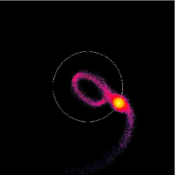
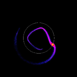
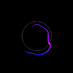
Figure 8: As in Figure 7 but comparing the ejecta at $T=4.0$ for the massive, low-mass, and tiny-mass satellites from left to right, respectively.

We show the tail morphology for our satellites with three different masses (see Table 1) on circular orbits at $T=4$ in Figure 8. The tidal tails in the low-mass and tiny-mass satellites ($0.001$ and $0.0001M_{host}$, respectively) very roughly follow the satellite orbit, with the leading and trailing tail located inside and outside of the satellite orbit. Compared to Figure 3, it is clear that the differences decrease with the satellite mass. As we described in Section 2, the low-mass satellite corresponds to the Sagittarius dwarf spheroidal galaxy halo and the tiny-mass satellite corresponds to the Draco dwarf spheroidal galaxy halo.

Figure 9: The evolution of the mean radius (top panel) and satellite potential (lower panel) for an ensemble of particles randomly selected from the leading tails in Figure 8 for the massive (solid), low-mass (dotted), and tiny-mass (dash-dot) satellites.

Figure 9 shows the evolution of the distance from the host halo centre and the satellite’s gravitational potential for an ensemble average of 10 randomly sampled particles near the tip of the leading tail in the three satellites. The tail from a massive satellite receives a larger torque and a larger shift to smaller energies and angular momentum than the tail from a lower-mass satellite. The bottom panel in Figure 9 shows that the decay results from interactions with the satellite potential. Figure 9 also shows that the satellite potential remains important in the low-mass and tiny-mass satellites when the tail is close to the satellite but it is unimportant when the tail is far from satellite. The satellite potential always remains significant for the massive satellite tail. The long-term influence of the satellite on the tail morphology makes any inference of the satellite orbit from the tidal tail impractical, especially for satellites on non-circular orbits (see Section 3.2.2).

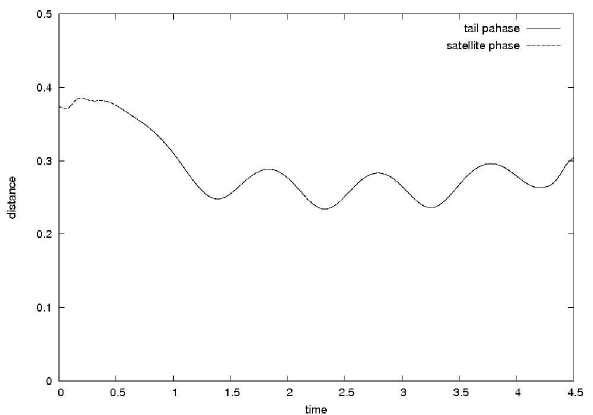
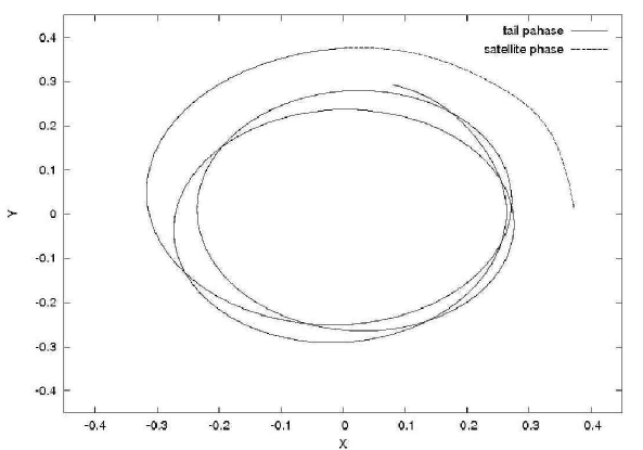
Figure 10: As in Figure 4 but now including the gravitational force of the satellite at all times. This force significantly lowers the energy and angular momentum of the leading orbit, decreasing its mean and apocentric radius. This initial period of deceleration ($T<1$) is responsible for the observed ‘kink’ in the tail (see Figure 8).

The leading tail from the low-mass and the tiny-mass satellites in Figure 8 exhibits kinks. The kinks are a consequence of the epicyclic motion of the tail orbits and of acceleration by the satellite at subsequent apocentres. Figure 10 shows the ensemble averaged distance and positions for a sample of leading tail particles orbits taken from the low-mass satellite simulation shown in Figure 5. The kink occurs at the first apocentre of the ejecta, after it is decelerated by the satellite during and subsequent to its escape. The deceleration during escape tends to correlate the phases of the ejected orbits and results in a narrowing of the tidal tail’s width. In contrast, the satellite potential accelerates the trailing tail particles, which increases the peri- and apocentres of the trailing tail. The analogous kink in the trailing tail is not so obvious because of its lower orbital frequencies. However, a plot analogous to Figure 10 does show a similar oscillation with lower angular frequency.

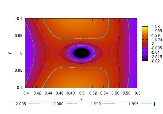
(a) $5\times 10^{-4}$

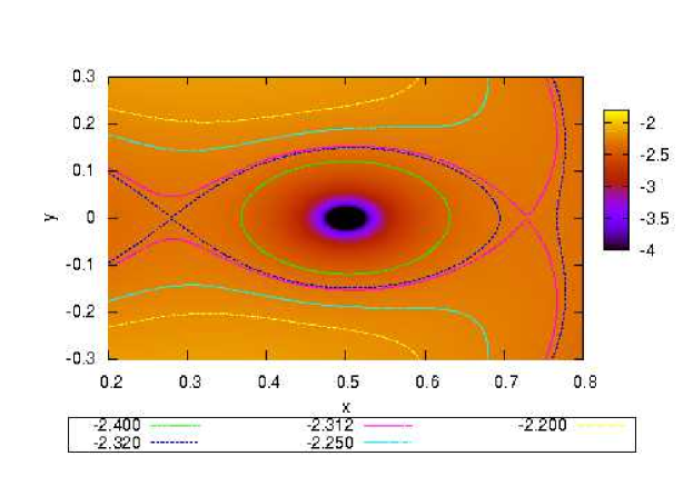
(b) $5\times 10^{-2}$

Figure 11: Contours of the Jacobi constant for two satellites with different masses as labelled. They follow a circular orbit with a radius of $q_{s}=0.4$ in a $c=15$ NFW halo of $M_{h}=1$ and a virial radius $R_{h}=1$. The $x$-axis describes the distance between the host halo centre and the satellite centre and the $y$-axis describes the location in the direction of orbital motion. Note the strong asymmetry in $x$ about the centre for the higher mass satellite in Panel (b).

The large changes in the orbits of escaping particles orbits are easily understood using a restricted three-body approach. Consider a satellite of mass $M_{s}$ in circular orbit at galactocentric radius $r_{s}$ in a halo of mass $M_{h}$. In the frame of reference moving with a satellite of vanishingly small mass, the effective potential is symmetric about the satellite centre. Although orbital energy and angular momentum are not conserved, this system admits a conserved quantity, the Jacobi constant:

$$E_{J}=E-\vec{\Omega_{s}}\cdot\vec{L}$$ (1)

where $E$ and $\vec{L}$ are the orbital energy and angular momentum and $\vec{\Omega_{s}}$ is the satellite’s angular frequency about the host halo. This expression is easily derived by identifying a perfect time derivative in the inner product of the velocity vector and Newton’s equations of motion in the rotating frame of reference (Binney & Tremaine, 1987, Section 3.3.2). An isocontour of the Jacobi constant passes through the X-points, $r_{\times}$, and demarcates the bound and unbound trajectories as shown in Figure 11a. As the satellite mass increases, the inversion symmetry about the satellite centre is broken and the unstable points separate as shown in Figure 11b. For small-mass satellites, therefore, the tidal force is symmetric about the satellite centre leading to symmetric tidal tails as seen in globular clusters. However, for large-mass satellites, the asymmetry in the tidal force leads to asymmetric mass loss.

Now consider the mass lost through the inner (outer) critical point, $r_{\times}$. Such orbits will have an inward (outward) velocity and unbound values of the Jacobi constant. The force from the satellite continues to affect the orbit beyond the tidal radius in this restricted problem as in the N-body simulations. Moreover, the smaller the mass of the satellite, the closer the radius is to that of the satellite, and the ejected orbit lingers near the original satellite orbit, partly offsetting the smaller gravitational force. For this reason, the orbit does not take on the orbital actions of the satellite but continues to be torqued by the satellite. One may estimate the scaling of this energy change by computing the work done in the satellite frame on the escaping tail particle; this naturally takes into account the lingering. Begin with the standard restricted three-body problem with generalised forces. Assuming that the satellite orbits in the $x$-$y$ plane and using Hamilton’s Equations, one may compute the $z$-component torque on an escaping particle and the change in angular momentum of the escaping particle after an interval $T$ becomes

$$\Delta L_{z}=\int_{0}^{T}dt\,\left(-{\partial H\over\partial\phi}\right)=\int_{0}^{T}dt\,\left(-{\partial V_{s}\over\partial\phi}\right)$$ (2)

where $H$ is the Hamiltonian, $\phi$ is the azimuthal coordinate conjugate to $L_{z}$ and

$$V_{s}=-{GM_{s}\over|{\bf r}-{\bf r}_{s}(t)|}$$

is the gravitational potential of the satellite. The second equality in Equation (2) owes to the $\phi$ independence of all the other terms in $H$. We may consider an escaping orbit in the limit that the mass of the satellite $M_{s}$ is much smaller than the mass of halo $M_{h}$ and use perturbation theory to evaluate Equation (2). To do this, let the unperturbed orbit be the circular orbit that passes through the X-point, $r_{\times}$ at $t=0$. Expanding to lowest contributing order in $M_{s}/M_{h}$, after some straightforward algebra and taking the limit $T\rightarrow\infty$, one may show that

$$\Delta L_{z}={GM_{s}\over r_{\times}^{2}}\left(\left.{\partial\Omega_{\phi}\over\partial r}\right|_{r_{s}}\right)^{-1}$$

where $\Omega_{\phi}$ is the azimuthal orbital frequency. Finally, it follows that $\Delta E=\Omega_{s}\Delta L_{z}$ from the conservation of the Jacobi constant (Equation 1) which yields:

$$\Delta E=-2\Omega_{s}^{2}r_{s}^{2}\left(-\left.{\partial\ln\Omega_{\phi}^{2}\over\partial\ln r}\right|_{r_{s}}\right)^{-1/3}\left({M_{s}\over M_{h}}\right)^{1/3}.$$ (3)

Since $G$, $r_{s}$, and $\Omega_{s}$ are constant, Equation (3) implies that the work done is proportional to $(M_{s}/M_{h})^{1/3}$. In other words, the change in the orbital energy of the escaping particle decreases as the satellite mass decreases but only weakly!

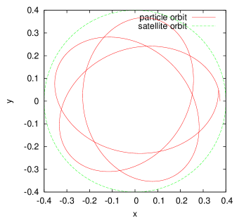
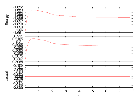
(a) inner

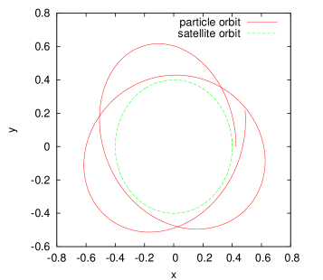
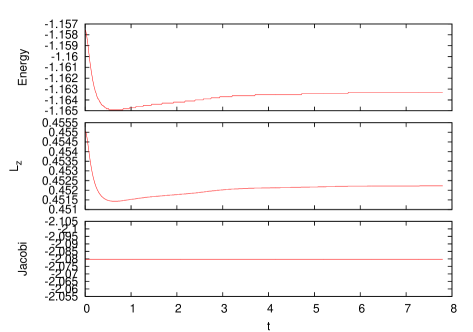
(b) outer

Figure 12: The evolution of two orbits escaping from the inner (upper panels) and the outer (lower panels) tidal radii for $M_{s}/M_{h}=10^{-4}$ where $M_{s}$ is the satellite mass and $M_{h}$ is the host halo mass. The left panels show the orbital plane and the right panels show the evolution of energy, angular momentum, and the Jacobi constant. The value of the Jacobi constant is conserved as expected.

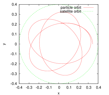
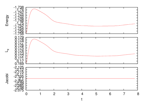
(a) inner

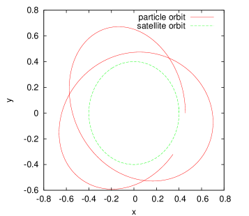
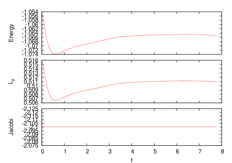
(b) outer

Figure 13: As in Figure 12 but for $M_{s}/M_{h}=10^{-3}$.

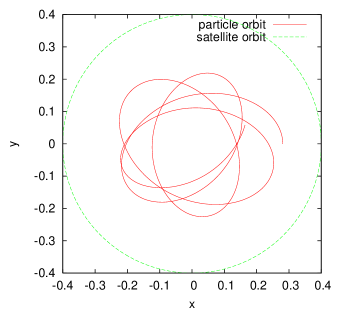
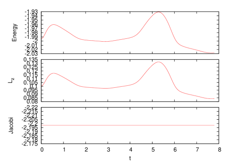
(a) inner

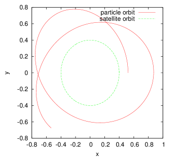
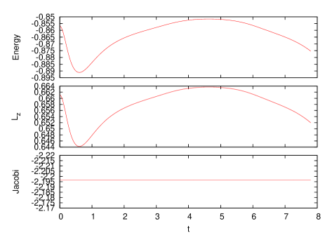
(b) outer

Figure 14: As in Figure 12 but for $M_{s}/M_{h}=10^{-2}$.

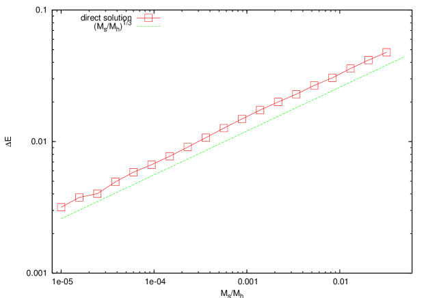
Figure 15: A numerical test of the predicted scaling of the energy change of escaping particles (Equation 3) with satellite mass. The $x$-axis is the ratio of satellite mass $M_{s}$ to total halo mass $M_{h}$ and the $y$-axis is the magnitude of the energy change, $\Delta E$. The straight line is the relation $(M_{s}/M_{h})^{1/3}$.

Figure 16: The time evolution of the energy, $E$, and the Jacobi constant, $E_{J}$, for two ensembles of particles ejected from the low-mass satellite selected from the leading and trailing tail, respectively. The value $E_{J}$ is nearly conserved while the energy changes owing to work done during escape. Changes in $E_{J}$ are caused by mass loss and the resulting evolution of the satellite’s gravitational potential.

Although the derivation of the scaling assumes $M_{s}/M_{h}\rightarrow 0$, we demonstrate numerically that it applies over all values of interest by integrating the equations of motion in the rotating potential. We adopt $r_{s}=0.4$ and choose values of the Jacobi constant that are 1% larger than the critical value passing through $r_{\times}$ with zero velocity. The initial motion, in the rotating frame, is along (or against) the direction of rotation for inner (outer) escapees. Figures 12–14 show the resulting trajectories and conserved quantities for $M_{s}/M_{h}=10^{-4},10^{-3},10^{-2}$. For inner (outer) escapees, the energy and angular momentum decrease (increase) after the initial transient for $t<0.5$. Figure 15 shows that the energy change for ensembles of orbits in the leading tail chosen as follows. The initial position is chosen to be 2% of $r_{\times}$ outside of the X-point and the velocities are chosen to have a normal distribution in the satellite frame with a dispersion that is 2% of the satellite’s circular velocity at $r_{\times}$. The orbits in Figures 12–14 are representative members of these ensembles. The magnitude of the energy change $\Delta E$ is defined as the ensemble average of $|E_{min}-E_{init}|$ where $E_{init}$ is the initial energy and $E_{min}$ is the minimum energy along the orbit. These numerical values are consistent with the predicted scaling $(M_{s}/M_{h})^{1/3}$. Circumstance may eventually bring the ejected particle close to the satellite once again, as seen in Figure 14. The radial extent of the annulus covered by the orbit increases only gradually with increasing satellite mass, reflecting the same weak dependence on $M_{s}/M_{h}$. In the simulations, the mass loss and subsequent reequilibration of the satellite potential causes small deviations in the Jacobi constant even though the satellite orbit remains circular as shown in Figure 16. Nonetheless, the restricted three-body dynamics explains most of the features seen in the orbit evolution.

3.2.2 Non-circular orbits

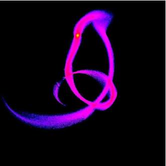
Figure 17: Tails at time $T=5.0$ for the massive (left) and the low-mass (right) satellite on an eccentric, $e=0.5$, orbit.

Although we still expect some of the insight gained from the restricted three-body problem to carry over to the evolution of a satellite on an eccentric orbit, this more complex situation requires direct simulation. Figure 17 shows the tidal tails of a massive and low-mass satellite on an eccentric, $e=0.5$, orbit. The tidal tail morphology for eccentric satellite orbits is significantly more complex than for circular satellite orbits and varies more strongly with satellite mass. In the left panel of Figure 17, the massive satellite has dramatically decelerated the leading tail, which now reaches the host halo centre and forms an inner “reservoir” of ejecta. The deceleration by the satellite causes the leading tail to appear close to radial. In the right panel of Figure 17, the multiply segmented tail from the low-mass satellite is caused by two mechanisms. First, during each satellite orbit, the leading tail forms during the approach to pericentre. After pericentre, the tidal strain and the mass-loss rate diminishes resulting in a gap in the tail. Second, deceleration by the satellite changes the orbits of the newly disconnected leading tail, producing a distinct segment.

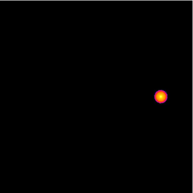
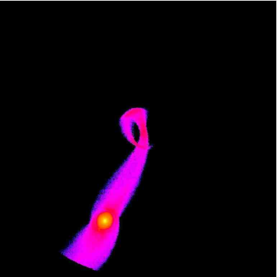
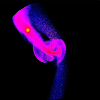
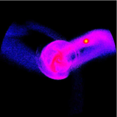
Figure 18: As in Figure 7 but for the massive satellite on an $e=0.74$ orbit at $T=0.0$, $1.5$, $3.0$, and $4.5$ in the top-left, top-right, bottom-left panels, and bottom-right panels, respectively.

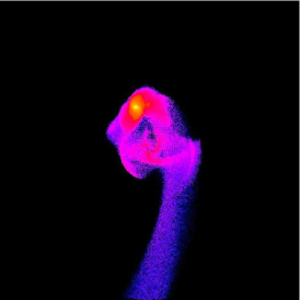
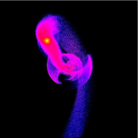
Figure 19: The same as Figure 18 but for times $T=2.5$, $2.75$, and T=$3.0$ from left to right, respectively, as the the satellite moves from pericentre to apocentre. Owing to the deceleration by the satellite potential, the leading tail falls toward the centre of the host halo.

Figure 18 shows the evolution of a massive satellite on an e=0.74 orbit. Initially, the leading tail points directly toward the halo centre but the strong deceleration by the satellite eventually fills the inner halo with ejecta. Figure 19 provides a finer time sampling of the evolution between pericentre and apocentre for the same simulation. Instantaneously, the morphology can be very complex and the position angle of the leading tail can vary significantly from its nearly radial average. There is little correlation between the tail location and the satellite orbit. The location of the inner ejecta, e.g. its outer turning points, is determined by the host halo potential, the time-varying satellite potential, and the satellite orbit in combination. Therefore, unlike streams from very low-mass satellites, the tail orientation is not directly informative. However, through dynamical modelling, the location of the inner ejecta may provide constraints on combinations of satellite properties and its history, and the galaxy potential.

4 Observational applications

We have demonstrated that tail morphology depends sensitively on the satellite mass and orbit. For modest to high-mass satellites, the ejected tails have orbits that differ significantly from that of the progenitor satellite. In this section, we illustrate the observational implications of these results.

4.1 Projected satellite tail morphology

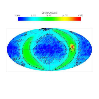
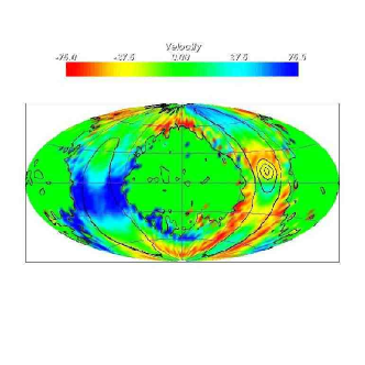
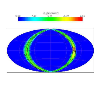
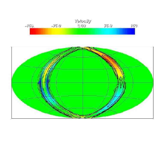
Figure 20: Aitoff projections of the massive satellite (top panels) and the low mass satellite (bottom panels) on an $e=0.5$ orbit. The snapshots for these projections are shown in Figure 17. The observer is located at the centre of the host halo. The left panels show the number density of particles and the right panels show the mean radial velocity. The black isocontours in all four panels represent the particle number density. Colour bars show the number density (left) and radial velocity (right) scales.

The observational implications for Milky Way streams can be summarised by projecting the tail star counts and radial velocity signatures against the sky with the observer at the centre of host halo. Figure 20 shows Aitoff projections of number density and mean radial velocity for the massive satellite (top panels) and the low-mass satellite (bottom panels) with an $e=0.5$ orbit (the same simulations described in Figure 17 at the same time, $T=5.0$). The Aitoff projection covers the entire sky, $0^{\circ}\leq l\leq 360^{\circ}$ and $-90^{\circ}\leq b\leq 90^{\circ}$, and the pixel size is $4^{o}\times 4^{o}$. The number density of the particles (left panels) and the mean radial velocity (right panels) are coded by colour. The contours in all the panels represent the particle number density. Velocity outliers at low number density are trimmed by setting to ${\bar{v}}_{r}=0$ all the pixels with fewer than 10 particles. The satellites are located at $l\approx 270^{o}$ and $b\approx 0^{o}$ and move in the positive $b$ direction.

The radial velocity signatures of the massive and low-mass satellites are distinctly different. These qualitative differences are a direct consequence of the large energy and angular momentum changes of the ejecta orbits leading to the phase wrapping of the leading tail and the dramatic broadening of the trailing tail (see Section 3.2.2). This causes the lower overall mean velocity values with a more rapid angular variation around the sky. In contrast, the mean velocity of the leading and trailing tails for the low-mass satellite are smooth and slowly vary around the sky. Quite clearly, the debris from the massive satellite will not show the distinct kinematic and spatial signatures that have been exploited in recent observational campaigns.

Near $b=0^{\circ}$ and $l=90^{\circ}$, one observes a region of receding orbits surrounded in longitude by regions of approaching orbits. Figure 17 (right snapshot) shows that line-of-sight projections will encounter strong leading and trailing tails from same satellite at different radii. The closer the tail to the observer, the larger the angular extent perpendicular to the motion of the stream. Their velocity signature in the Aitoff projection occurs as a single line of sight cuts through these tails at different radii.

The Aitoff projections contain most of the information that one might obtain from combined kinematic–photometric surveys such as RAVE (Steinmetz et al., 2006). In particular, these results show that tail morphology depends on satellite mass. Therefore, a wide range of kinematic “template” models may be required to best exploit the information implicit in observed halo stars.

4.2 The effects on tidal tail radial velocity

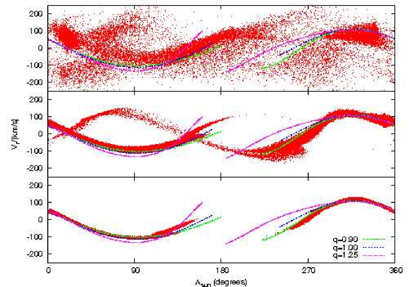
Figure 21: The radial velocity of tail particles as a function of orbital longitude for the massive satellite, low-mass satellite, and tiny mass satellite, from top to bottom, shown in Milky Way units. All three satellites have orbits with $e=0.5$ and are centred at a longitude of $0^{o}$. The width of the distribution in $|v_{r}|$ increases with satellite mass. For comparison, the satellite trajectories for halos with flattenings of $q=0.9,\>1.0,\>1.25$ are also shown. Although all three simulations are performed in a spherical host halo potential, the tail locus is better matched for a satellite trajectory with $q=0.9$.

Radial velocity–orbital longitude diagrams are frequently used to characterise large-scale kinetic features in the Milky Way. Figure 21 shows radial velocity–orbital longitude diagrams for the ejecta of satellites with orbits having $e=0.5$ for each of our three masses. We convert simulation units to Milky Way units by assuming a virial radius of 250 kpc and a total mass of $1.0\times 10^{12}M_{\odot}$ (Klypin et al., 2002). In Figure 21, the Sun has ${\bf R}=(-8.0,0.0,0.0)$ kpc and the Galactic plane and the satellite’s orbital plane are coincident. Here we adopt the Sagittarius longitudinal coordinate system described in Majewski et al. (2003) for the orbital longitude. All satellites have ${\bf R}=(50.0,-7.5,0.0)$ kpc and move in the $y$ direction. Therefore, the satellite has $l\approx 0^{\circ}$ and longitude increases along the trailing tail (in the $-y$ direction). The radial velocity is measured from the halo centre. The spread in $|v_{r}|$ is proportional to the satellite mass, as expected from the previous discussion and hence the mean velocity will be an unbiased diagnostic of the satellite orbit only for very low mass satellites. Although we have only modelled the dark matter, it is likely that the $v_{r}-l$ space distribution for stellar and dark matter ejecta will be similar in most cases since the internal satellite velocity dispersion plays only a minor role in shaping the ejecta distribution.

Law et al. (2005) use M giants from the Two Micron All-Sky Survey (2MASS, Skrutskie et al., 2006) to map the position and velocity distributions of tidal debris from the Sagittarius dwarf spheroidal galaxy. Assuming that tidal tails approximately align with the satellite trajectory, the authors note that the radial velocity distribution of tidal debris suggests an prolate Milky Way halo with an axis ratio of $q=c/a=1.25$. However, our results demonstrate that the tails do not follow the satellite orbit. In Figure 21, we also plot satellite trajectories for three different halo flattenings to compare with the particle distributions of our simulations evolved in a spherical host halo. Following Law et al. (2005), we flatten our host halo parallel to the satellite’s motion and compute point-mass satellite trajectories to compare with our simulated $v_{r}-l$ diagrams. Surprisingly, the distributions of the low-mass satellite and the tiny-mass satellite tidal tails most closely matches a $q=0.9$ halo. The gravitational acceleration by the satellite shifts the tail location in the radial velocity distribution and this trend is degenerate with the effects of halo flattening. For instance, the location of the leading tails decelerated by a massive satellite is degenerate with the trajectories of tails in an oblate halo with no satellite deceleration. We have not attempted to model the Milky Way in sufficient detail to estimate the halo flattening including satellite deceleration. However, the degeneracy between halo flattening and the shift caused by the satellite gravitational acceleration suggests that the Law et al. (2005) conclusions may be biased and a more careful analysis including the full dynamics of the halo-satellite interaction is necessary.

4.3 The effects on the tidal tail phase space distribution

Several groups have proposed phase-space-based detection diagnostics for moving groups associated with disrupted dwarf galaxy and star cluster streams. Lynden-Bell & Lynden-Bell (1995) proposed using the intrinsic correlation of moving groups’ radial energy and galactocentric radius to identify disrupted systems. The procedure is as follows. Assuming a spherical gravitational potential for the outer galaxy, one estimates the radial energy $E_{r}=v_{r}^{2}/2+\Phi(r)$ and the galactocentric radius $r$ of the putative ejecta stars from observations. Then, assuming that all of the debris from a single satellite has the same orbital energy, $E$, and angular momentum, $L$, conservation of energy implies a simple linear relationship in $r^{-2}$: $E=E_{r}-L^{2}/2r^{2}$. Hence, linear features in the observed $E_{r}$–$r^{-2}$ diagram indicate the detection of a tidal stream. Recently Belokurov et al. (2007) used this method to support the detection of stellar streams in the Sloan Digital Sky Survey.

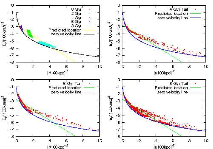
Figure 22: Radial energy, $E_{r}=v_{r}^{2}/2+\Phi(r)$, plotted against inverse galactocentric radius, $r^{-2}$, for the low-mass satellite with an $e=0.5$ orbit. Particles with the same energy and angular momentum as the satellite will lie on a particular straight line. The zero velocity curve describes the lowest possible energy at a given radius for this host halo. The material bound to the satellite follows the straight locus at all times (top left). The escaped particles are shown at $T=2.0$ (top right), $T=3.0$ (bottom left) and $T=4.0$ (bottom right), respectively. Only one particle out of 250 are plotted for visibility. Because the leading (trailing) tail loses (gains) energy, the ejecta deviates from the predicted straight line with significant scatter. Times in Gyrs are scaled to the Milky Way.

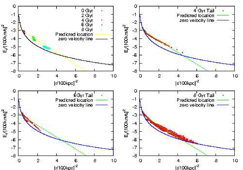
Figure 23: The same as Figure 22 but for the tiny-mass satellite.

However, as we have now seen, a massive satellite will modify the conserved quantities of the ejecta orbits and change their location in $E_{r}-r^{-2}$ space. Figures 22 and 23 show the $E_{r}-r^{-2}$ diagrams for the low-mass and tiny-mass satellite simulations on an $e=0.5$ orbit. For clarity, we have reduced the point density by randomly sampling the simulation phase space and plot the bound particles at five different times in the upper-left panels. We calculate the expected linear relation from the satellite’s initial position and velocity. The bound material in low-mass and tiny-mass satellites lies along the predicted linear relation at all times. We plot the tail particles at three different times in the other three panels. As one can see in Figure 22, the deviation of the tail particles from the predicted locus and the scatter in $E$ at fixed $r^{-2}$ for the low-mass satellite is large. Especially at late times, e.g. the bottom right panel in Figure 22, the tail nearly fills the region between the zero velocity curve and the predicted locus. However, one can see from Figure 23 that tail particles from the tiny-mass satellite do follow the predicted linear relation. Therefore, we conclude that the Lynden-Bell & Lynden-Bell (1995) diagnostic can only detect streams from very low-mass satellites such as globular clusters.

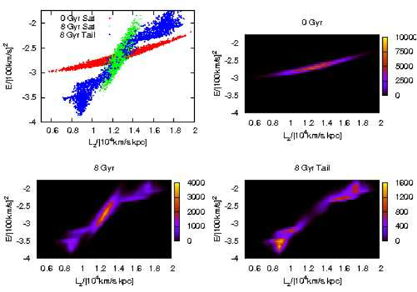
Figure 24: The distribution of particles bound to the low-mass satellite on an $e=0.5$ orbit and its ejected tail particles plotted in $E$–$L_{z}$ space. Top left: The phase-space distribution at $T=0.0$ and $T=4.0$ for the bound satellite and its tail (subsampled as in Figure 22). Density plots of the phase-space distribution are shown at $T=0.0$ (top right), at $T=4.0$ (bottom left) and at $T=4.0$ for the ejected tail particles alone (bottom right).

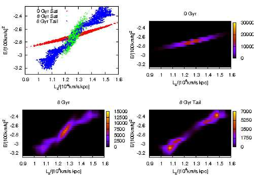
Figure 25: The same as Figure 24 but for the tiny-mass satellite

Motivated by the prospect of six-dimensional phase-space data from future astrometric missions, Helmi & de Zeeuw (2000) proposed to identify phase-mixed satellite debris by a cluster analysis in $(E,L,L_{z})$ space. We explore the consequences of tail evolution on this approach using the same two simulations in Figure 24 for the low-mass satellite and in Figure 25 for the tiny-mass satellite. For simplicity, we assume that we know the orbital orientation and consider only the $E$–$L_{z}$ projection. The top-left panels show the distribution at 0 Gyr ($T=0$) and at 8 Gyr ($T=4$) when scaled to the Milky Way halo in $E$–$L_{z}$ space. Once again, we randomly sampled the material to improve clarity. The top-right and bottom-left panels show density estimates in $E$–$L_{z}$ space for the satellite at 0 Gyr and at 8 Gyr, respectively. In the bottom-right panels we show the density of only the tail particles at 8 Gyr. The overall position of the satellite and its tail changes little from 0 Gyr to 8 Gyr, although the shape of the distribution shifts. In both figures, there are two or more peaks at high and low energy with respect to the satellite owing to decelerations and accelerations of tail particles by the satellite potential. Moreover, the tidal field is nonaxisymmetric and this leads to spatial correlations in the energy and angular momentum of the least bound satellite particles, which in turn leads to the production of several apparently disassociated phase-space clumps before disruption.

5 Discussion and summary

The observational detection of “S”- or “Z”-shaped tidal tails in globular clusters (e.g. Leon et al., 2000; Odenkirchen et al., 2003; Grillmair & Dionatos, 2006) promises sensitive statistical tests of the Galaxy’s gravitational potential and has renewed the quest for streams from larger satellites. For globular clusters, i.e. very low mass satellites, the tidal tail morphology is easily interpreted. (Capuzzo Dolcetta et al., 2005; Montuori et al., 2007) However, for massive satellites, the bisymmetry that leads to this simple morphology is broken by the interaction of the host halo’s gravitational field and the self-gravity of the satellite itself. We present new dynamical aspects and morphologies of tidal tails produced in satellites of significant mass, $M_{s}/M_{h}\geq 0.0001$. There are two dynamical principles that affect the tail production for massive satellites. First, the leading and trailing X-points, points where the attractive force of the host halo and satellite are balanced at zero velocity, do not occur at equal distances from the centre nor do they have the same equipotential value for large-mass satellites (see Figure 11). Second, the escaped ejecta in the leading (trailing) tail continues to be decelerated (accelerated) by the satellite’s gravity leading to large offsets of the ejecta orbits from the satellite’s original orbit (see Figure 17). We show that this is consistent with Hill-Jacobi theory (generalised to dark-matter halos) for satellites on circular orbits. In particular, the effect of the satellite’s self gravity on the tail decreases only weakly with decreasing satellite mass, proportional to $(M_{s}/M_{h})^{1/3}$ (see Section 3.2.1) and, therefore, the acceleration by the satellite after escape is important for dwarfs and dark halos of modest mass.

These findings have several important and useful theoretical and observational consequences. First, for a finite mass satellite, the morphology of the leading and trailing tails will be different owing to the gradient in the underlying halo potential across the satellite. In addition, the tail ejection occurs over a range of azimuth relative to the X-point owing to the dynamical response of the originally prograde and retrograde orbits to the tidal and non-inertial acceleration. These effects should be observable in high resolution imaging for both dwarf spheroidal and globular clusters (see Figs. 17–19).

Second, the radial velocity of tail particles will be displaced from that of the satellite orbit. The magnitude of the displacement is proportional to the satellite mass. These trends distort the ejecta from the gravitationally bound satellite trajectory in the $v_{r}-l$ plane in much the same sense as a satellite trajectory in a flattened halo (see Figure 21). In other words, in fitting the $v_{r}-l$ diagram for tidal tails to satellite orbits of different flattenings, the satellite mass is covariant with halo flattening, i.e. the shape parameter $q=c/a$. Therefore, a constraint on the Milky Way halo shape using tidal streams requires mass-dependent modelling. Finally, the acceleration of ejecta by a massive satellite during escape spreads the velocity distribution and obscures the signature of a well-defined “moving group” in phase space (see Figs. 22–25).

Although we believe that the physical effects described in this study are robust, our intentionally idealised simulations ignore several possibly relevant processes. First, the dynamical friction and the self-gravitation of the tail are ignored, although in all but the most extreme mass satellites their effects on the tail morphology will be negligible, since the mass in the tail is very small. Second, we assume a smooth and static spherical host halo potential. In reality, over time, as the host halo mass grows its shape may change, and the ejecta will be perturbed by substructure. These time dependent effects will not affect the applicability of the dynamics described here but will complicate the prediction of observational signatures. Finally, we have not included the physics of a dissipational baryonic component that may have slightly different kinematics than that of a dark collisionless component. In spite of these shortcomings, our study elaborates the details of satellite tidal tail production and the dynamics that bear on the interpretation of observed streams.

As an example, Moore & Davis (1994) and Johnston et al. (1996) find that satellite tails follow the satellite orbit for dwarf galaxies whose mass is negligible compared to the galaxy mass. The mass of these satellites is usually similar to or less than our tiny-mass satellite. Using these simulation results, Johnston et al. (2001) developed an efficient numerical method to investigate the detectability and interpretation of tidal debris tails. However, we have demonstrated here that the gravity of the satellite for $M_{s}/M_{h}\geq 0.0001$ will change the actions of the tidal ejecta to mimic halo flattening (see Section 4.2, Figure 21). In addition to the spatial distribution, the velocity distribution of the tail is affected by the satellite potential (see Section 4.3). We would like to note that (Fujii et al., 2006) have also noticed a systematic distance offset for leading (trailing) tails inside (outside) the orbit of a satellite owing to the satellite potential. However, they did not focus on the tail morphology.

In summary, we have shown that the interplay between the satellite and the host halo results in a complex tail morphology whose amplitude scales weakly with mass. Although these findings complicate the interpretation of stellar streams and moving groups, the intrinsic mass dependence provides additional leverage on both the halo and on the progenitor satellite properties. A statistical study of these trends will further constrain the dark halo potential and the mass accretion history of the Milky Way.

References

- Belokurov et al. (2007) Belokurov V. et al., 2007, ApJ, 658, 337
- Binney & Tremaine (1987) Binney J., Tremaine S., 1987, Galactic dynamics. Princeton, NJ, Princeton University Press, 1987
- Bryan & Norman (1998) Bryan G. L., Norman M. L., 1998, ApJ, 495, 80
- Capuzzo Dolcetta et al. (2005) Capuzzo Dolcetta R., Di Matteo P., Miocchi P., 2005, AJ, 129, 1906
- Clutton-Brock (1972) Clutton-Brock M., 1972, Ap&SS, 16, 101
- Clutton-Brock (1973) Clutton-Brock M., 1973, Ap&SS, 23, 55
- De Lucia et al. (2004) De Lucia G., Kauffmann G., Springel V., White S. D. M., Lanzoni B., Stoehr F., Tormen G., Yoshida N., 2004, MNRAS, 348, 333
- Diemand et al. (2004) Diemand J., Moore B., Stadel J., 2004, MNRAS, 352, 535
- Fujii et al. (2006) Fujii M., Funato Y., Makino J., 2006, PASJ, 58, 743
- Gao et al. (2004) Gao L., White S. D. M., Jenkins A., Stoehr F., Springel V., 2004, MNRAS, 355, 819
- Ghigna et al. (1998) Ghigna S., Moore B., Governato F., Lake G., Quinn T., Stadel J., 1998, MNRAS, 300, 146
- Ghigna et al. (2000) Ghigna S., Moore B., Governato F., Lake G., Quinn T., Stadel J., 2000, ApJ, 544, 616
- Grillmair & Dionatos (2006) Grillmair C. J., Dionatos O., 2006, ApJL, 641, L37
- Gunn & Gott (1972) Gunn J. E., Gott J. R. I., 1972, ApJ, 176, 1
- Hayashi et al. (2003) Hayashi E., Navarro J. F., Taylor J. E., Stadel J., Quinn T., 2003, ApJ, 584, 541
- Helmi & de Zeeuw (2000) Helmi A., de Zeeuw P. T., 2000, MNRAS, 319, 657
- Helmi & White (1999) Helmi A., White S. D. M., 1999, MNRAS, 307, 495
- Hernquist & Ostriker (1992) Hernquist L., Ostriker J. P., 1992, ApJ, 386, 375
- Ibata et al. (2001a) Ibata R., Irwin M., Lewis G., Ferguson A. M. N., Tanvir N., 2001a, Nature, 412, 49
- Ibata et al. (2001b) Ibata R., Lewis G. F., Irwin M., Totten E., Quinn T., 2001b, ApJ, 551, 294
- Ibata & Lewis (1998) Ibata R. A., Lewis G. F., 1998, ApJ, 500, 575
- Johnston et al. (1996) Johnston K. V., Hernquist L., Bolte M., 1996, ApJ, 465, 278
- Johnston et al. (2001) Johnston K. V., Sackett P. D., Bullock J. S., 2001, ApJ, 557, 137
- Johnston et al. (1999) Johnston K. V., Zhao H., Spergel D. N., Hernquist L., 1999, ApJL, 512, L109
- Klypin et al. (2002) Klypin A., Zhao H., Somerville R. S., 2002, ApJ, 573, 597
- Law et al. (2005) Law D. R., Johnston K. V., Majewski S. R., 2005, ApJ, 619, 807
- Leon et al. (2000) Leon S., Meylan G., Combes F., 2000, A&A, 359, 907
- Lindegren & Perryman (1996) Lindegren L., Perryman M. A. C., 1996, A&AS, 116, 579
- Lynden-Bell & Lynden-Bell (1995) Lynden-Bell D., Lynden-Bell R. M., 1995, MNRAS, 275, 429
- Majewski et al. (2003) Majewski S. R., Skrutskie M. F., Weinberg M. D., Ostheimer J. C., 2003, ApJ, 599, 1082
- Majewski et al. (2004) Majewski S. R. et al., 2004, AJ, 128, 245
- Mayer et al. (2002) Mayer L., Moore B., Quinn T., Governato F., Stadel J., 2002, MNRAS, 336, 119
- Montuori et al. (2007) Montuori M., Capuzzo-Dolcetta R., Di Matteo P., Lepinette A., Miocchi P., 2007, ApJ, 659, 1212
- Moore & Davis (1994) Moore B., Davis M., 1994, MNRAS, 270, 209
- Navarro et al. (1997) Navarro J. F., Frenk C. S., White S. D. M., 1997, ApJ, 490, 493
- Odenkirchen et al. (2003) Odenkirchen M., Grebel E. K., Dehnen W., Rix H.-W., Yanny B., Newberg H. J., Rockosi C. M., Martínez-Delgado D., Brinkmann J., Pier J. R., 2003, AJ, 126, 2385
- Oguri & Lee (2004) Oguri M., Lee J., 2004, MNRAS, 355, 120
- Perryman et al. (2001) Perryman M. A. C., de Boer K. S., Gilmore G., Høg E., Lattanzi M. G., Lindegren L., Luri X., Mignard F., Pace O., de Zeeuw P. T., 2001, A&A, 369, 339
- Skrutskie et al. (2006) Skrutskie M. F. et al., 2006, AJ, 131, 1163
- Steinmetz et al. (2006) Steinmetz M. et al., 2006, AJ, 132, 1645
- Stoehr et al. (2002) Stoehr F., White S. D. M., Tormen G., Springel V., 2002, MNRAS, 335, L84
- Weinberg (1999) Weinberg M. D., 1999, AJ, 117, 629
- Weinberg & Katz (2007a) Weinberg M. D., Katz N., 2007a, MNRAS, 375, 425
- Weinberg & Katz (2007b) Weinberg M. D., Katz N., 2007b, MNRAS, 375, 460
- Zentner et al. (2005) Zentner A. R., Berlind A. A., Bullock J. S., Kravtsov A. V., Wechsler R. H., 2005, ApJ, 624, 505