Spatial decomposition of on-nucleus spectra of quasar host galaxies

Abstract

In order to study the host galaxies of type 1 (broad-line) quasars, we present a semi-analytic modelling method to decompose the on-nucleus spectra of quasars into nuclear and host galaxy channels. The method uses the spatial information contained in long-slit or slitlet spectra. A routine determines the best fitting combination of the spatial distribution of the point like nucleus and extended host galaxy. This is fully complementary to a numerical spatial deconvolution technique that we applied to the same data in a previous analysis, which allows a cross-calibration of the two methods. Inputs are a simultaneously observed PSF, and external constraints on galaxy morphology from imaging. We demonstrate the capabilities of the method to two samples of a total of 18 quasars observed with EFOSC at the ESO 3.6m telescope and FORS1 at the ESO VLT. $\sim$50% of the host galaxies with sucessful decomposition show distortions in their rotation curves or peculiar gas velocities above normal maximum velocities for disks. This is consistent with the fraction from optical imaging. All host galaxies have quite young stellar populations, typically 1–2 Gyr. For the disk dominated hosts these are consistent with their inactive counterparts, the luminosity weighted stellar ages are much younger for the bulge dominated hosts, compared to inactive early type galaxies. While this presents further evidence for a connection of galaxy interaction and AGN activity for half of the sample, this is not clear for the other half: These are often undistorted disk dominated host galaxies, and interaction on a smaller level might be detected in deeper high-resolution images or deeper spectroscopic data. The velocity information does not show obvious signs for large scale outflows triggered by AGN feedback – the data is consistent with velocity fields created by galaxy interaction.

1 Introduction

After having been a fascinating but bizarre species of astrophysical objects for three decades, quasars have shifted into the mainstream focus of galaxy evolution. When the tight relation between black hole masses and masses of the galaxies hosting them became evident (e.g., Ferrarese & Merrit, 2000) it was clear that there is a mechanism leading to an effective co-evolution of galaxies and their central black holes. Quasars, accreting black holes, might be the key to understanding the extent and physics of this co-evolution, or at least of the phase in which the black holes grow strongest.

In a second role, the energy feedback of quasars via galactic winds currently provides an alternative possibility beside supernova feedback to expell gas from galaxies and quench star formation. Quasar activity might be responsible for the switching off of star formation and the onset of evolution of massive galaxies towards the red sequence of ellipticals.

For both roles vital information is still missing before the question about cause and effect in co-evolution can be settled, the same is true for the frequency of outflows in quasars, their properties, and the effect on the interstellar medium (ISM) in the host galaxies. In the end both roles might be the two sides of the same complex mechanism.

Most studies of quasar host galaxies in the past were restricted to imaging. For investigating e.g. morphologies, companion statistics, interaction states, luminosity distributions, imaging is well suited. High resolution imaging with ground based telescopes or the HST (e.g., Bahcall et al., 1997; Sánchez et al., 2004; Jahnke et al., 2004b; Floyd et al., 2004) provided most of todays knowledge on quasar host galaxies.

However, many techniques applied to the investigation of normal, inactive galaxies require SED information in the shape of colours or even spectra. Determination of e.g. stellar populations, velocity measurements, ionisation states of the ISM can, by their nature, not be performed on imaging data. So spectral information is not only appreciated, but in the face of fundamental questions as ‘Is nuclear activity part of any galaxie’s life cycle?’, ‘What triggers nuclear activity?’ or ‘How far does co-evolution go?’ it is urgently needed.

In a recent article (Jahnke et al., 2004a) we described a method to extract coarse but robust spectral information on QSO host galaxies. Coarse, because by using broad band imaging we sample the SED of a QSO in our case in seven wavelength intervals between 4000 Å and 23000 Å. The broad band filters integrate over several hundred or thousand Å, in order to collect significant amounts of light.

The method showed to be robust, because by now the uncertainties and caveats of semi-analytic two-dimensional image modelling are quite well understood. Software has been developed and tested, by us (Kuhlbrodt et al., 2004) and other groups (e.g., Peng et al., 2002; Floyd et al., 2004), and the problems of PSF and host modelling have been investigated in depth (e.g., Kuhlbrodt et al., 2004; Jahnke et al., 2004b; Sánchez et al., 2004; Jahnke et al., 2006). Thus the implemented modelling scheme is powerful and has assessable uncertainties, as was demonstrated in several articles.

In spectroscopy the situation is different. Spectroscopic studies of the host galaxies of broad-line, type 1 QSOs are very difficult: The AGN in the centre overpowers the host galaxy’s emission much more strongly than in broadband imaging, because the narrow slit is integrating much of a compact nucleus and little of an extended galaxy. Until recently it was not possible to access host spectra directly around the nucleus at all, where the connection between host and nucleus is strongest.

1.1 Previous studies and fundamental problems

Very few spectroscopic studies were attempted, knowing too well of the problems of the task. In the 30 years of host galaxy research before 2006 only about 25 articles were published on quasar host galaxy spectroscopy – compared to more than 100 on imaging –, and more than half of those appeared before 1985.

Between the mid 70’s and mid 80’s pioneering spectroscopic work was done, confirming the cosmological nature of the QSO redshift (Wampler et al., 1975; Stockton, 1976; Richstone & Oke, 1977; Wyckoff et al., 1980), and establishing the presence of gas emission lines and later stellar continuum and absorption lines underneath the nuclear glare (Morton et al., 1978; Green et al., 1978; Wyckoff et al., 1980; Boroson & Oke, 1982; MacKenty & Stockton, 1984).

The first larger sample was investigated in a series of papers by Boroson, Oke & Green (1982), Boroson & Oke (1984) and Boroson, Persson & Oke (1985), which also remained the largest study for almost 20 years. Two characteristic groups of hosts were classified there, with either blue continua and strong gas lines, or continua with weak or absent gas emission. The authors found positive correlations of this classification with the shape of the nuclear Balmer lines, the strength of the nuclear [O III] emission, the strength of Fe features, absorption line strength, radio spectrum shape and radio morphology. Later studies found evidence for star formation possibly induced by tidal events (MacKenty & Stockton, 1984; Hutchings & Hickson, 1988), coordinated rotation of gas in the host (Hickson & Hutchings, 1987; Hutchings & Crampton, 1990), and an extention of the gas emission beyond the continuum (Hutchings & Hickson, 1988).

The next level of detail took ten more years when Canalizo & Stockton (2000) performed a deep, spatially resolved study of the host galaxy of 3C 48. The analysis included modelling the stellar content of 32 regions of the host. They found strong evidence for recent starburst of 5 to 100 Myrs and old evolved stars in other parts, fitting well into the picture of a merger event going on in 3C 48. This result is supported by – or rather vice versa the study was initiated because of – the tidally disturbed structure of the object visible in imaging.

At the same time a study aimed to compare the stellar populations of radio-quiet QSOs, radio-loud QSOs and radio galaxies (Hughes et al., 2000; Nolan et al., 2001) – the objects investigated were part of an earlier well studied imaging sample (Dunlop et al., 1993; Taylor et al., 1996; Dunlop et al., 2003). Model fitting showed evolved stellar populations, with only small contributions to the light from recent star-formation, corresponding to young stars of less then about one percent of the visible mass. The samples however, were manually selected to match in different properties, as luminosity and redshift range, and contained extremely massive galaxies, thus it is difficult to assess in which properties these are representative for the general host galaxy population.

In the recent past, a number of publications used the wealth of the Sloan Digital Sky Survey (SDSS) as an AGN database for host galaxy studies. While most of them focussed on type 2 quasars or rather Seyferts, particularly to mention the large study of Sy 2 by Kauffmann et al. (2003) and of type 2 QSOs (Zakamska et al., 2003; Zakamska et al., 2005), only recently studies (Hao et al., 2005; Dong et al., 2005; Vanden Berk et al., 2006) tackled SDSS broad-line AGN, using an spectral eigenvector decomposition technique. Type 2 AGN have, from their lack of a directly visible central source, no contamination problem in the first place. However, they only tell half of the story: The central source can not be studied directly, black hole masses can only be estimated indirectly from the velocity dispersion or luminosity of their host galaxy – without the possibility of an independent calibration. In addition, the obscuring material might be different or differently distributed at different luminosities. Particularly, few proper type 2 quasars are known. Until the unified model of type 1 and 2 is confirmed, and also to confirm it, studies of the more difficult to analyze type 1 QSOs are required.

Aside from the mentioned studies from the SDSS, in all other work on type 1 AGN the host spectra were either taken with the slit directly “on-nucleus”, but were strongly contaminated by nuclear light, or taken “off-nucleus”, at distances of several arcseconds from the centre, to sample regions of the host as far away as possible from the nuclear light.

Two problems arise from this: Firstly, a distance of 5″as e.g. used by Hughes et al. (2000) corresponds to a linear distance of $\sim$20 kpc at $z=0.2$ – as a consequence, the slit does not sample the central regions of the host galaxy. Secondly, despite the 2–5″distance of the slits from the nucleus there remains a nuclear contribution, scattered into the slit by the seeing. These nuclear contributions were in the abovementioned studies either not corrected or it was attempted to remove them by subtracting a scaled on-nucleus spectrum that was assumed to contain only nuclear light. As in the case of one-dimensional spatial host galaxy image separation, the amount of nuclear light to be subtracted is not known a priory. The only knowledge lies in that the stellar continuum does not contain broad emission lines. So increasing amounts of on-nucleus spectrum were subtracted, modified with an ad-hoc function of wavelength, until the broad lines (typically H$\alpha$ and/or H$\beta$ ) were removed. This method is often imperfect and can not remove the contribution completely and leaves unwanted residual flux (e.g. Hutchings & Crampton, 1990).

In summary, with off-nucleus spectra neither can the astrophysically most interesting central parts of host galaxies be sampled, nor does this approach guarantee the absence of artefacts like nuclear residuals in the resulting spectra.

1.2 On-nucleus data: the test cases

To avoid these drawbacks, we acquired on-nucleus slit spectroscopy data for two samples of broad-line quasars at two different telescopes and instruments, EFOSC at the ESO 3.6m telescope and FORS1 at the ESO VLT (sample summary in Tab. 1). Such on-nucleus data require, before analysis, that the contributions of nucleus and host galaxy have to be separated in the data processing stage to access the host galaxy information. In order to do this, we developed two complementary techniques. In this article we present for one of the techniques both the working principles, as well as summarize the most important science results from these two datasets. The other, complementary deconvolution technique was applied to data from the same VLT-campaign (extended by a second semester, doubling the number the ten objects analysed here to 20), and we published the results in more detail in a series of other papers (Courbin et al., 2002; Letawe et al., 2004; Magain et al., 2005; Letawe et al., 2006, see below,).

The extraction of the host galaxy spectrum is made possible by these two independent and new techniques that allow to separate the host from nuclear light, making use of the so far unused spatial dimension of long-slit spectra. These methods allow to estimate the host SED directly from on-nuclear long slit spectra, without prior assumptions about the resulting host spectrum, and allow a spatially resolved investigation directly down to the centre.

The first method is the spatial numerical deconvolution of the two-dimensional (2d) composite spectrum developed by Courbin et al. (2000), already mentioned above. The other is a simultaneous semi-analytic spatial modelling of nucleus and host spectrum, which we describe in the following. Both methods are based on the same principles – using the spatial information contained in 2d spectra – yet the algorithmic approach is different and complementary. Courbin et al. are deconvolving the spatial component of the spectrum into a point source and an extended source, using a modified version of their algorithms for imaging deconvolution (Magain et al., 1998). Using the two techniques on the the same VLT dataset, allows a comparison of the techniques for identical input data.

Our previous work focused on spatial deconvolution of the data. We are now investigating a fundamentally different approach, with semi-analytic two-component spatial PSF fitting of the 2d-spectra. In the following we will describe the general principles of the method and detailed implementation. In section 6 we present the application of this method to one example object for each of the two different qualities of spectroscopic data taken with ESO 3.6m EFOSC and VLT FORS. In section 7 we summarize the scientific results we extracted from the two datasets.

A discussion of the capabilities and limits of the modelling technique is given in section 8.

2 2d decomposition of spectra

It is possible to numerically disentangle host galaxies from the active nucleus. For spectroscopy this is more difficult than for imaging, because of the additional parameter wavelength $\lambda$, and less S/N at each $\lambda$ point than in broadband imaging. Our approach is to incorporate as much external information into the separation process as possible. “Information” in this case means knowledge about the QSO, like morphological host galaxy parameters, the shape of the PSF or other information from imaging. We combine this with using all spatial information available in 2d longslit spectra. Up to now this information was never used for the extraction of host galaxy spectra.

2.1 Different instruments and data types

Optical and NIR spectral information can be obtained with a multitude of instruments and techniques. Beside classical long slit spectroscopy, currently several types of multi-object spectrographs are available. Units like the multi object spectroscopy unit (MOS) of FORS on the ESO VLT use movable slitlets of fixed length, or use exchangeable masks that are individually manufactured for each observation (e.g. at the ESO VLT for the FORS2 and VIMOS instruments). Slitlets and masks in general have the same capabilities as long slits, with an additional degree of freedom when targetting more than one object in the field of view.

All of these spectroscopy techniques have in common that spectral and spatial information are obtained simultaneously. For host galaxy applications the spatial information can be used to disentangle the spectral components of an active nucleus and host galaxy. The approach described below can be used with long slit, slitlet, or mask spectra (we have recently also modified this principle to integral field spectroscopy, see Sánchez et al., 2006).

2.2 General approach

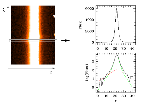
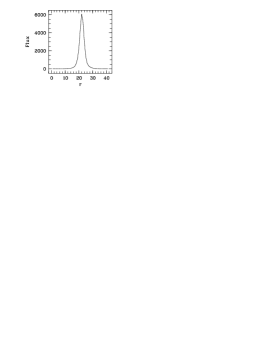
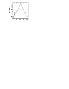
Figure 1: Schematic view of modelling: 2d-spectrum (left) with spatial direction horizontally, and dispersion direction vertically. For each row the composite spatial surface brightness distribution is modelled (top right). Bottom right shows the logarithm of the total surface brightness distribution from above (solid, black) with best fitting models of nucleus (dashed, green) and host (dotted, red).

The spatial component of long slit spectra is often collapsed after reduction (for quasar hosts e.g. by Hughes et al. 2000 and Nolan et al. 2001) to extract the full object flux. For extended objects like galaxies, however, the spatial direction can be used to study the galaxy spatially resolved, in our case along a slice through the centre of the QSO. Thus instead of collapsing the spatial dimension after data reduction, we use the 2d-frames with dispersion and spatial direction during the complete process of separation.

Our general approach to separate active nucleus and host galaxy is very similar to the imaging case described in Jahnke et al. (2004a): For each wavelength element $\lambda$ (e.g., a row of the 2d spectrum in Fig. 1), the spatial 1d surface brightness distribution of the QSO consists of a superposition of point source like nucleus and extended host. The shape of the point source is defined by the shape of the PSF at the time of observations and at the position of the QSO on the chip at the specific wavelength.

In our approach we first model the spatial shape of the PSF and then build models for the combined light distribution of both the nucleus and the host, asuming a certain analytic shape for the host. A fitting procedure determines the best set of parameters for these models. Due to the low S/N per individual wavelength element, a simultaneous fit of all parameters (e.g. centres, shape parameter, fluxes, etc.) will not be well constrained. We thus exploit external input knowledge on the host to constrain as many parameters as possible, thus reducing the number of free parameters in each fit. We also exploit that some of these parameters vary only slowly with $\lambda$, to reduce noise. After a parameter has been fitted, it is fixed in the following modelling steps until in the final step only the central surface brightnesses of nucleus and host are free parameters. In this way the fitting routine makes optimal use of the signal, the introduction of additional noise is minimised and the fits can succeed.

The 2d decomposition consists of the following steps, which in the following we will describe in detail:

• Spatial definition of the PSF with the fit of an analytical funtion to each row of a PSF star. This includes centering, determination of a Moffat shape parameter $\beta$ and width $\alpha$ for all $\lambda$. $\longrightarrow\mathrm{PSF}(x,\lambda)$

• Creation of an analytical look-up-table correction, to account for intrinsic differences in the shapes of PSF model and the “true” PSF, using the residual of the PSF modelling. $\longrightarrow\mathrm{LUT}(x,\lambda)$

• Simultaneous spatial modelling of nucleus, represented by the determined PSF, and the host, represented by a exponential disk or de Vaucouleurs spheroidal.

  • First the center is determined, and its variation with $\lambda$ fitted. $\longrightarrow x_{0}(\lambda)$

  • Morphological type and width of the host are determined externally from broad band images. $\longrightarrow$ type and $r_{1/2}$

  • In a final step the fluxes of nuclear and host model are fitted with all other parameters fixed.

• If possible, emission lines are modelled separately to avoid numerical flux transfer from nucleus to host model.

3 PSF definition

The first step of the modelling is estimating the PSF. With current instruments it is not possible to satisfy all three requirements: to know the PSF at the position of the QSO on the chip, at the wavelength in question, and at the time of observation. However, with everchanging ambient conditions the temporal variations are large, and due to the dependence of the PSF on wavelength, the wavelength condition is also crucial. In comparison the variation of the PSF within the FOV is small for current multi-purpose instruments. Thus the best results will be reached when defining the PSF at the same time and wavelength regime as the QSO observation. This is realised by simultaneously observing a PSF star with the QSO, a requirement that can be realised with longslit or multi-object spectroscopy, and many targets.

If the spatial variations in the end are sufficiently small depends not only on the instrument and its specific optical distortion pattern, but also on the distance of the PSF star from the main target, the contrast of nucleus and host galaxy, and the quality of externally input information about host galaxy shape. Absolute statements are difficult to make: For faint AGN in bright galaxies and small seeing the PSF will more often be sufficiently well described than for compact systems and large seeing. With PSF variations of a few percent, host galaxy light of less than a few percent of the total flux will be out of reach. The brighter and spatially closer the PSF star is to the target quasar, the better. We have a number of targets in section 6 and 7 for which the combination of conditions is not fulfilled and we can not separate successfully. While depending on the exact science goal, we see no principle obstacle to use any modern spectrograph for this type of science.

We describe the PSF as a combination of an analytical function and an empirical correction, and do not use the empirical PSF star directly, for three reasons: Firstly, the analytic approach allows to recenter the PSF to different (sub-pixel) positions without any broadening. Secondly, the convolution on a fine grid is substantially faster and more straightforward than with an empirical PSF, because the empirical correction – which is small and has small gradients – can simply be added in the end. Last but not least, while we did not yet implement this, the analytical approach in principle allows to model spatial PSF variations if more than one PSF star is observed with the target.

The PSF modelling process schematically consists of:

• centering

• global functional form determination

• width determination

• creation of an empirical look-up-table correction

3.1 Parametric description

The PSF is characterised by using a parametrised functional form, fitted for each $\lambda$. Different functional forms could be used. A single Gaussian has only one free shape parameter (width), but is too simple to describe real world PSFs. We opted to use a Moffat profile (Moffat, 1969), which showed to match well in earlier imaging studies we performed with focal reducer instruments (Kuhlbrodt et al., 2004). The expected and measured differences between the Moffat functional shape and the observed PSFs are small and are taken care of by the empirical correction (section 4.2). Other functional descriptions could have been used, e.g. two Gaussians, with then somewhat different empirical look-up-table corrections, but without substantial differences in the resulting PSF.

In the Moffat profile

$$\mathrm{PSF}(x)=I_{0}\left[1+\left(\frac{x-x_{0}}{\alpha^{\prime}}\right)^{2}\right]^{-\beta}.$$

$x_{0}$ is the centre of the function, the parameter $\beta$ describes the “winginess” of the profile, the relation of flux contained in wings compared to the nucleus. $\alpha^{\prime}$ is a measure of the width of the Moffat. We use a modified description

$$\mathrm{PSF}(x)=I_{0}\left[1+\left(\frac{x-x_{0}}{\alpha}\right)^{2}(2^{1/\beta}-1)\right]^{-\beta}$$

that makes $\mathrm{FWHM}=2\alpha$.

For $\beta\rightarrow\infty$ the Moffat function reduces to a Gaussian. Atmospheric turbulence theory predicts a shape for the seeing that can be fitted with $\beta=4.765$ (Saglia et al., 1993; Trujillo et al., 2001), although real data show larger wings (lower $\beta$) due to telescope imperfections. Tests for our image modelling showed a good fit of the shape to the data in most cases. We find a range of $1.8<\beta<3.5$ for the spectroscopic data.

3.2 Centroid $x_{0}$

The centroid of an observed object on the detector chip will vary with wavelength, when the object is not observed in the paralactic angle. Because of the constraints on rotator angle imposed by the orientation of the long slit or slitlet unit this is generally not possible. Thus first of all the centroid is determined for each $\lambda$. For this task a Moffat function is fitted at each wavelength, though any symmetric function showing a maximum in the centre could be used (see below). We use a Moffat function with $\beta$ and width $\alpha$ set to initial values, and allow the centroid $x_{0}$ and the central flux as free parameters.

Finding the best centroid is done in two iterations. First we use a numerical Levenberg-Marquard least square algorithm (Press et al., 1995) with no subsampling of the initial pixels, to get a robust initial estimate for $x_{0}$. After repeating this for all $\lambda$ we use the fact that $x_{0}$ is varying only very slowly with wavelength. Thus changes between adjacent rows will be of the order of 1/100th of a pixel in a high resolution 2d spectrum. We use this fact by fitting a polynomial of typical degree 3–7 to the raw $x_{0}(\lambda)$ to strongly reduce the noise (Fig. 2).

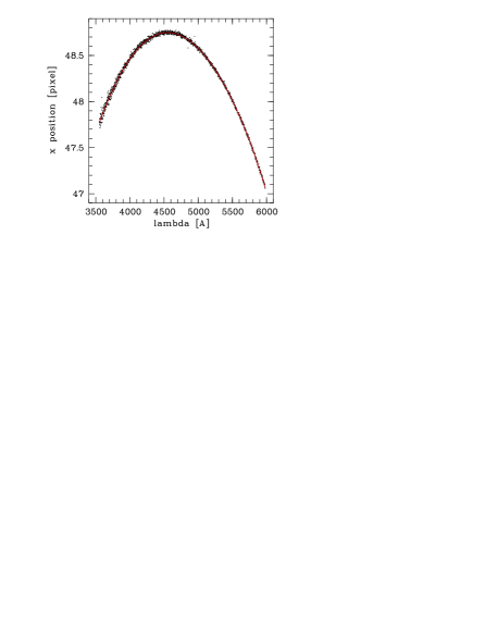
Figure 2: Example of PSF star centering: Plotted are the individually determined centres for each $\lambda$ (dots). The solid line is a polynomial of degree 7 fitted to the points. This $x_{0}(\lambda)$ is used as the best estimate for the centre in the following modelling steps.

The second iteration uses these centroids as input for a downhill simplex algorithm (Press et al., 1995) that again determines a centroid value. As for the imaging case described in Jahnke et al. (2004a) we now use a division into a finer subpixel grid to compute the PSF model to avoid artifacts from defining the function only on the comparably coarse pixel grid. The number of subpixels is in general only limited by computing power. For the strong gradients in case of a narrow PSF, it is advisable to use at least 50 subpixels. Beyond 50 subpixels the improvements become negligible.

After this step again a polynomial is fitted for $x_{0}(\lambda)$, using the Levenberg-Marquard fit result as a zero-line for clipping outliers. This relation is now being used as the best estimate for $x_{0}(\lambda)$. In the next steps $x_{0}(\lambda)$ is fixed to this relation and is no longer a free parameter. In this way centering precisions of the order of 1/100 of a pixel are possible.

As mentioned above, for the inital centering it is not important to know the shape parameter $\beta$ and the width $\alpha$ precisely. As the PSF can be assumed to be symmetrical, the centering will yield good results, as soon as the initial width estimate is in the right ballpark. For $\beta$ an initial value of 2.0–2.5 is usually appropriate. The initial guesses for width and central flux as well as the degree of the smoothing polynomials have to be chosen individually for each spectrum.

3.3 Shape parameter $\beta$

The next step after centering is to estimate a global value for the parameter $\beta$ of the Moffat function. Within limits the general shape of the PSF, i.e. the “winginess” of the Moffat function, should not change with wavelength. In any case the PSF shape is not perfectly described with a simple two-parameter function, thus residuals are to be expected (they are attempted to be removed with an analytical look-up-table, described later in section 4.2). Tests show that $\alpha$ and $\beta$ are directly correlated when fitting a given shape (Fig. 3), thus a $\beta$ changing slightly with $\lambda$ can be compensated by a different width $\alpha$, without dramatically worsening the quality of the fit.

With fixed $x_{0}(\lambda)$ we compute global reduced $\chi^{2}$-values, i.e. cumulated for all $\lambda$, for different values of $\beta$, with $\alpha$ and central flux as free parameters in a downhill simplex fit. A bracketing algorithm is used to find the global $\beta$ with the lowest resulting $\chi^{2}$ and subsequently $\beta$ is held fixed. If we assume that the PSF were constant over the FOV, $\beta$ is then valid for PSF and QSO as it describes the functional form of any point source at the time of observation.

However $\beta$ might change for different objects, i.e. time of observation, and also different grisms. We did not find a systematic dependency on central grism wavelength, thus we conclude that the changing ambient atmospheric conditions dominate the value of $\beta$ if certain conditions are met. We discuss these conditions and the influence of the PSF star brightness below in section 4.1.

3.4 Width $\alpha$

As for the centering, the width $\alpha(\lambda)$ is determined in two steps. Centroids $x_{0}(\lambda)$ and $\beta$ are now fixed to their best estimates, and only $\alpha$ and central flux remain as free parameters. Using global initial guesses, first a robust Levenberg-Marquard fit without subsampling is used for each $\lambda$, followed by a polynomial smoothing fit. Then this relation is input as an initial guess for a fully subsampled downhill simplex fit, again followed by a polynomial fit over $\lambda$ with clipping of outliers. The width is changing faster with $\lambda$ than the centroids (see Fig. 3), over the whole spectroscopic range changes of 30% were observed for some objects. The change seems to be mainly due to a change in shape due to the different atmospheric refraction, depending on wavelength.

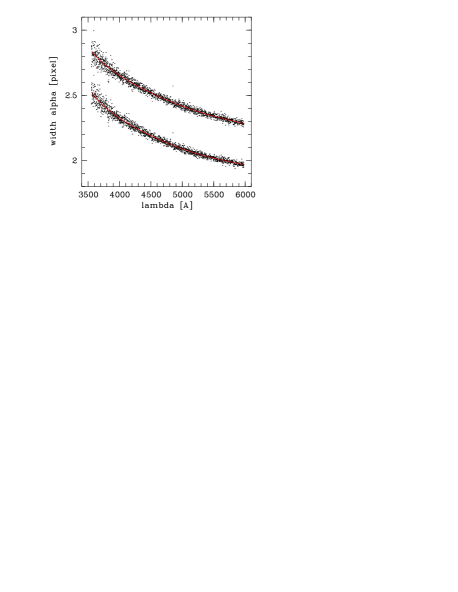
Figure 3: Example of fitting the width $\alpha$ for a PSF star: Dots are again the individually determined $\alpha$ values for each $\lambda$. The solid line is a polynomial fit. This $\alpha(\lambda)$ is used as the best estimate for the width of the PSF in the QSO modelling steps. As an illustration for the correlation of $\alpha$ and $\beta$ the fits for two values of $\beta$ are given. Top: $\beta=3.5$, bottom: $\beta=1.75$. There is a systematic offset of $\Delta\alpha\sim 0.3$, changing slowly with $\lambda$.

4 PSF variations

At this point all parameters $\beta$, $x_{0}(\lambda)$, and $\alpha(\lambda)$ are determined. With this stepwise approach the effects of noise and numerical artifacts are minimised. However, we initially requested as a third requirement to estimate the PSF at the position of the QSO in the FOV, not at the position of the PSF star. In imaging, we notice variations of the PSF parameter over the FOV, so how strong is the effect in 2d spectroscopy?

Here the problem is simpler compared to imaging: we only have one, not two spatial coordinates. Thus the variation of ellipticity, position angle and width of the PSF is effectively reduced to a variation of the width. Any change in the other spatial coordinate has only an effect across the width of the slit and thus a (negligible) influence on the spectral coordinate, and none on the spatial.

In the usual case that very few PSF stars are observed simultaneously with the QSO, in many cases only a single one, it is not possible to model PSF shape variations over the field. For crowded fields this is a theoretical posibility. The magnitude of the variation will depend on the instrument and its optical layout. We performed a comparison for one of our objects (see end of next section) that showed that the effects are not very large in this case. In section 6.1 we will comment on focal reducer type instruments, and their general PSF instability.

4.1 Sensitivity to $\beta$ and S/N effects

Two further sources for errors in the PSF shape are the sensitivity to the exact value of $\beta$ and dependence on the brightness or S/N of the PSF star. Both effects are connected. With decreasing S/N the wings of the PSF will more and more vanish in noise, thus the wings will have less weight in the fit. We already noted the correlation of width $\alpha$ and shape parameter $\beta$ (Fig. 3). When determinining the shape of the PSF star for decreasing S/N, $\beta$ will increase and so will $\alpha$, leading to a similar just less wingy shape. So there are two separate effects to be investigated: Variations in shape due to a different $\alpha$–$\beta$ combination, e.g. due to different S/N, and variations in shape for a fixed $\beta$ and different S/N. The first appears when PSF star and QSO nucleus differ strongly in brightness. The second is valid for every PSF star, because a global $\beta$ is determined, but the flux and thus S/N varies with $\lambda$.

An analysis of the residuals after removal of the PSF model shows the magnitude of the effects: If for a given PSF star $\beta$ is varied by $1.75\leq\beta\leq 3.5$, which represents the complete range of $\beta$ values found for our whole sample observed with VLT FORS, the differences in the residuals can be significant (Fig. 4). For any single object the possible range in $\beta$ can be established much better. For a range of $\Delta\beta<0.1$ the difference is of the order of one $e^{-}$/pixel, thus for a “good” bright PSF star this is small compared to the total PSF star flux.

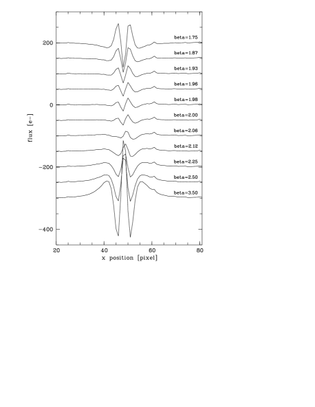
Figure 4: Dependence of the PSF residual on the shape parameter $\beta$. Plotted is the spatial residual averaged over all wavelengths for the PSF star of HE 0956–0720 (grism 600B) for different values of $\beta$. The curves are offset for better visibility. The magnitude of the residual has to be compared to a central flux of the PSF star of in this case 4600 $e^{-}$, or 180 times more than the structures in the best fit ($\beta=1.98$). Size and structure of the residual vary from object to object.

We also tested the change in $\alpha$ for different S/N and a fixed $\beta$, which simulates different brightness of PSF star and nucleus. In a frame where two PSF stars of different brightness were available, we fixed $\beta$ and determined the width $\alpha$ for both stars. In a test case with a difference in brighness of a factor of three, the widths are virtually identical down to the low S/N regime of the spectrum. The only difference in the mean relations is due to a non-gaussian scatter of the individual $\alpha(\lambda)$ points for the fainter star, but the magnitude is not significant. With consistent shapes down to this level, we can expect it to be well defined for all $\lambda$ with substantial flux. Quantified as a S/N, one should be on the safe side with a S/N in the central pixel of $>$20.

This agrees well with results for simulated PSF stars of different S/N. We created a noiseless model PSF star with known width, added noise for different amounts of sky background and fitted the width with the technique described above. We used 0.15, 1.0, 7.1 and 71.0 times the typical sky background noise for our objects. The width does change systematically, but a very good reconstruction of the width better than 5% can be found for S/N of the central pixel of better than 10–20. In the modelling of the EFOSC sample, further evidence was found that stars below a minimum S/N of $\sim$20 in the central pixel can create artificially large $\beta$ values, largely independent of ambient conditions.

4.2 Look-up-table correction

Besides variation of the PSF with S/N and position over the FOV, there is also a systematic mismatch between shape of the PSF star and its the two-parameter Moffat function model. The difference between PSF and model is the same for PSF star and QSO, assuming a constant PSF shape. We correct the majority of this mismatch by constructing an empirical look-up-table (LUT) correction, consisting of the modified residual of the PSF modelling process.

The residual is smoothed using a moving average along the dispersion direction, in order to reduce noise. This can be done because we assume the residuals forming the LUT to be strongly correlated in adjacent $\lambda$. In the same process it is normalised with the flux of the PSF star, and rebinned to match centre $x_{0}$ and $\lambda$ of the QSO.

Tests show that LUTs from different PSF stars vary in their details, but show a generally identical shape. The resulting LUT applies corrections on the order of a few percent, in the best cases less than 1%. Thus the second-order errors in LUT difference are very small.

In total we have a smoothed empirical correction function $\mathrm{LUT}(x,\lambda)$ to complement the analytical PSF description $\mathrm{PSF}(x,\lambda)$.

5 Modelling nucleus and host galaxy

Modelling the QSO follows the same principles used for the PSF star. Parameters are estimated, their variation with $\lambda$ fitted, and this relation fixed in subsequent steps, reducing the number of free parameters in each step as much as possible.

The centering is directly identical to the PSF modelling, using a single Moffat function. In all following steps two components are modelled: a PSF like component representing the nucleus and an extended component for the host. The S/N per wavelength element is generally so low that simultaneously determining parameters for a third component, e.g. gas disk or separate bulge, is not possible (but we will discuss this possibility for the treatment of emission lines in section 5.3). For the host we assume a one-dimensional exponential disk or de Vaucouleurs spheroidal profile, as in the imaging case, but in a one-dimensional form:

$$\mathrm{SPH}(x) = \mathrm{SPH}_{0}\exp\left[-7.67\,\left(\frac{\left|x\right|}{r_{1/2}}\right)^{1/4}\right]$$ (1)

$$\mathrm{DISC}(x) = \mathrm{DISC}_{0}\exp\left(-1.68\,\frac{\left|x\right|}{r_{1/2}}\right)$$ (2)

These models also have two parameters, central flux $I_{0}$ and half light radius $r_{1/2}$.

The creation of the spatial models is again done on a fine subpixel grid. For each point on this grid the value of the PSF is computed, as the sum of analytical Moffat function plus empirical LUT. The host model is convolved with the PSF as a discrete convolution at these grid points. After computation, the grid points are binned back onto the (coarser) pixel grid of the data frame. This convolution is the main reason for using a downhill simplex algorithm. As it has to be done numerically, no derivatives are available.

5.1 Scale length of the host galaxy

In the step after centering the half light radius and the galaxy type (disk/spheroidal) are determined. This can either be done via fitting, with $x_{0}(\lambda)$ fixed and $I_{0}$, $r_{1/2}$ and central flux of the nucleus as free parameters. But due to the low S/N this is a source for failure in many cases. The host can be outshone by the nucleus by a factor of 100 or more. In spectroscopy by sampling just along a slice through the QSO which contains most of the nuclear but only a small fraction of the host light, the total nucleus-to-host flux ratio is boosted. Wherever available, we use external information on host galaxy type and $r_{1/2}$ to overcome this problem, by obtaining an auxilliary image for any object and determining the morphological parameters as described in Jahnke et al. (2004a).

The price for a deep 2d image of a QSO host to determine morphological host parameters is small compared to the price of the spectrum itself. Thus for little extra observation time – for the redshift range accessible to this spectral modelling, $z<0.5$, one can use 2m-class telescopes, or invest 30–60 s of 8m-class time – the results are greatly enhanced, if not only made possible in many cases.

Thus the functional form and half light radius are set from external sources. As we noted in Jahnke et al. (2004a), the scale lengths of galaxies can be variable with $\lambda$ due to colour gradients. Because usually no multiband imaging data is available we have to assume it to be constant. $r_{1/2}$ and $I_{0}$ are strongly correlated parameters. Even though their individual values are not well constrained for low S/N, their product in the form of the total flux can be estimated with a much higher precision (Abraham et al., 1992; Taylor et al., 1996). Thus the quality of the fit and total host flux will not strongly depend on the exact value of $r_{1/2}$.

If $r_{1/2}$ should after all be taken from the spectrum, one way to increase the S/N is to coadd parts or all of the spectral dimension, with care taken about the varying centroid, and all emission lines omitted, and model the resulting 1d frame. In total the S/N of the host is greatly increased. Depending on S/N, even a varying $r_{1/2}$ could be determined by splitting the spectrum into two or more parts. This process can be done iteratively: Modelling is first done with an initial guess. The resulting host spectrum is used to extract a better spatial model to be used in the second iteration etc.

5.2 Final step: the host spectrum uncovered

In the final step just two parameters are free, the central fluxes of host and nucleus, with all other parameters fixed. The resulting model of the host is not used for further analysis, only the 2d nuclear model image is used as the best estimate for the nuclear component and subtracted from the initial 2d QSO spectrum. The result is a residual host galaxy frame on one hand including all PSF removal imperfections, but on the other hand containing all deviations from symmetry like rotationally shifted lines that are not modelled by the symmetric model, and differences in actual morphology.

This frame can now be subjected to standard 2d spectra calibration and analysis techniques. The 1d spectrum is extracted using the Horne optimal extraction algorithm (Horne, 1986).

5.3 Emission line treatment

Refinements have to be applied in the treatment of emission lines. While the broad emission, narrow emission and continuum of the QSO have an identical spatial shape, this is not the case for the host. The spatial distribution of the interstellar gas, responsible for narrow emission lines visible in the host, does not need to be identical to the distribution of stellar emission. This is particularly obvious in elliptical galaxies, where rotating gas disks can be embedded in the spheroidal distribution of stars.

This has the consequence that at wavelengths with a substantial contribution of gas emission lines, the two-component model of nucleus plus host is a wrong assumption. E.g. in the case of an elliptical galaxy with a gas disk, the gas emission will spatially be more extended and less peaked than the stellar emission. To account for the extra flux at larger radii the numerical algorithm will assign extra flux to the more extended of the two components, i.e. the host. This boosted host model will match the gas emission well at the radii in question, but will overestimate it in the center. This will be compensated by the nuclear model, that as a result will be underestimated.

Three solutions can be used, for different situations:

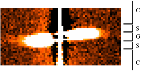
Figure 5: Emission line in a resulting host spectrum, dispersion vertical, spatial coordinate horizontal. The two sides are rotationally shifted in wavelength due to rotation of the gas disk. Three fundamentally different regions can be identified: Pure continuum emission (“C”), single sided emission line (“S”) and double sided gas emission (“G”). For all three regions different modelling conditions apply.

• Single sided modelling: In the case of a rotating gas disk, both sides of the line are rotationally shifted away from the nominal position, one side blueward, the other redward. In the case of a narrow line and a rotation curve that does not strongly decrease with radius, e.g. the case for gas disks in elliptical galaxies, only parts or even none of the single sided components overlap in wavelength (marked “G” in Fig. 5).

  In the non-overlap wavelength elements (marked “S”in the same figure) it is possible to model just one side of the 2d spectrum. With fixed PSF, $x_{0}$ and $r_{1/2}$, the nuclear model is determined just for the side free of line and only continuum emission. This nuclear model is then valid also for the other, line emission “contaminated” side of the spectrum. In this way an emission line with non-overlapping sides can be split up into two parts and the single sided nuclear models can be merged with the full models for all other $\lambda$.

• If the two sides of the line do have some overlap, the underestimate for the nucleus might be seen in the resulting spectrum. It could be manifested as a absorption like feature where none is expected, or as a disturbance in the spectrum. In this case the oversubtraction in the nucleus model can be estimated and a better nuclear contribution constructed. This however is difficult to judge.

• A third approach, not yet implemented, is the use of a third model component in the emission line. Here the S/N is large and the stellar continuum can be estimated from adjacent spectral intervals (marked “C” in Fig. 5). Even with nuclear contamination a good scale length for the gas disk can be obtained from the radial shape, when excluding the central spatial part of the line. The stellar contribution would enter only as a constant component. With a set gas component scale length, again only two free parameters, $I_{0}$ of nucleus and gas, would be present.

5.4 Continuum flux transfer

If two spatially different components exist in the object under investigation, and the S/N is sufficiently high, this modelling procedure will find those components. However, a signal of the host might be found only in the brightest parts of the spectrum, e.g. a narrow gas emission line, while the stellar continuum is outshone by the luminous nucleus. If the variation of the PSF is large and the host compact, errors in the PSF will be compensated by the routines with changes in the host model flux. As a result, more or less strong flux transfer can occur from the nucleus to the host or vice versa. This can go as far as negative fluxes for a part or all of the resulting host spectrum. In this case the errors in the PSF determination are larger than the positive signal of the host. When this happens, one can still extract some information from the resulting two component spectra, because the spectrum was still separated into a wider and a more compact component. A solution is to add increasing fractions of the nuclear component, possibly of wavelength dependent size, to compensate for the modelling error, and make the host flux positive again. After such a procedure, it will not be possible to extract detailed host continuum information, but host line ratios, rotation curves etc. can still be extracted to some extent.

5.5 Quality of fit diagnostics

Similar as for the PSF star modelling, the models used for the galaxy can never describe all of the data. Spiral arms, bulges in disk galaxies or asymmetries are not accounted for. Thus even with a LUT correction for the nuclear component, there can be substantial residuals of data minus best nucleus and host model. This is no particular problem as the modelling is only used to estimate the nuclear component. As long as the fit is “good”, the resulting model of the host is irrelevant. To asses the “goodness” and quality of a modelling run, six fundamentally different diagnostic principles are available:

• Boundary conditions: Some general boundary conditions from basic physical principles apply, that, when not hardwired into the modelling routine, can be used to check results. The most important are

  • host flux should be zero or positive for all $\lambda$, within the limits of noise,

  • forbidden lines cannot appear in absorption.

• The residuals of the fit can be used to detect misestimates of the host’s scale length. When comparing the residuals it is possible to discriminate between different scale length values. Too compact models show residual flux in the wings.

• The nuclear broad emission lines should not appear as strong mirrored absorption lines in the resulting host flux. Broadened absorption lines can occur in galaxy spectra, but not of a width of several 1000 km/s as the permitted nuclear emission lines.

• Broad band colours existing from imaging studies must be reconstructable within the errors of calibration.

• If more than one PSF star of suitable S/N exists, the results from modelling with both stars can be compared.

• Finally, if several images exist for the same object, taken with different grisms, the fit results in overlapping spectral regions can be compared agains each other.

It has to be kept in mind at all times that every algorithm, also the one described, is limited by S/N. It can not extract information that simply is not there.

6 Spectroscopic decomposition: example objects

Applying this method to actual data is the crucial test. We want to show the detailed results of one example from each dataset and summarize more of the science results after that.

All objects are low-$z$ quasars, $z<0.2$ and $z<0.3$ respectively for the EFOSC and FORS1 instruments with apparent total magnitudes from $V\sim 13.5\ldots 16.5$ (see Tab. 1). Integration times ranged from 20 min with FORS to typically 30–60 min with EFOSC, split up into several exposures. Slit sizes, spectral and spatial resolution were 2”/$\sim$250/0$\aas@@fstack{\prime\prime}$314 and 1”/$\sim$700/0$\aas@@fstack{\prime\prime}$2 for EFOSC and FORS respectively. For FORS three grisms were used to cover the range from 4000–8000 Å.

The MOS multi-object mode used with FORS was effectively used as a more flexible long-slit thus the data is not fundamentally different for those two data sets. In the observations the slit angle and mask layout were set so that at least one bright accompanying PSF star was observed simultaneously with the QSO in the longslit. The PSF star was chosen to be close to the object, bright, but not too bright to reach the non-linear regime of the detector or even saturate. The airmass for all observations was at or below 1.1.

The EFOSC sample is a subsample of the objects investigated with broad band imaging in Jahnke et al. (2004a). Thus apart from the astrophysical analysis this sample can be used to crosscheck the output of our modelling with results from broadband imaging. For the FORS objects only in the $H$ band decent data was available, the imaging observations are part of a different project (Kuhlbrodt, 2003). We chose the objects HE 0952–1552 ($z=0.108$, $V_{\mathrm{tot}}=15.8$, nucleus/host$(V)=1.2$, nucleus/host$(H)=0.6$) as an example for the EFOSC data quality and HE 1503+0228 ($z=0.135$, $B_{\mathrm{tot}}=16.3$, $H_{\mathrm{tot}}=13.6$, nucleus/host$(H)=1.5$) for FORS. Both objects are disk dominated.

6.1 PSF modelling

EFOSC and FORS are focal reducer type instruments. As is known the complex optical layout with multiple optical elements in the light path will produce geometric distortions in the focal plane and a shape of the PSF depending on position in the FOV. We investigated this effect in detail in Kuhlbrodt et al. (2004) for the imaging case, and in principle the same problem applies to the spectroscopy case. Here, however, we do not have the possibility to model these distortions by analysis of a large number of PSF stars – generally only one or two stars are observed. It can only be attempted to minimize the effects by observation design.

Generally, the difference in shape between two points in the FOV will increase with increasing distance. Therefore it is advisable to observe PSF stars as close as possible to the QSO. However, as noted in section 4.1, we require a minimum brightness for the stars, to reduce the uncertainty in PSF shape determination. Thus for most host galaxy studies there is only a small choice of stars to be used. For these samples it was attempted to find a good compromise between brightness of the star and the distance to the QSO. Generally instruments should be preferred that show a stable shape of the PSF. This can even be of higher priority than light collection power. Too strong variations can not be compensated by higher S/N. For our samples we found that the distortions in FORS are much small than for EFOSC, as expected for the younger and higher quality optics.

6.2 Decomposition results

Modelling was carried out as described in the previous sections. We used 80 subpixels per input data pixel in the spatial coordinate, and the LUTs were created by smoothing over a radius of 30 pixels in wavelength.

Figures 6 and 7 display the modelling results for each of the two example object, in the form of the extracted 1d spectra. The top panels show (from top to bottom) the original spectrum of the QSO (black), the model for the nucleus (red), the resulting host spectrum after subtraction of the nuclear model (green) and the residual after subtraction of nuclear and host model (blue). The bottom panels show a zoom of the host spectrum.

For both objects the modelling was straight forward without further manual intervention, i.e. the errors in PSF and host morphology estimation were small enough for the S/N, contrast and spatial resolution given. There are no obvious oversubtractions visible, i.e. flux transfer to the nucleus. The host spectra are void of nuclear broad lines, while the narrow line components in H$\alpha$ and H$\beta$ are clearly present. For HE 1503+0228 even some Balmer absorption can be detected underneath the narrow H$\beta$ line.

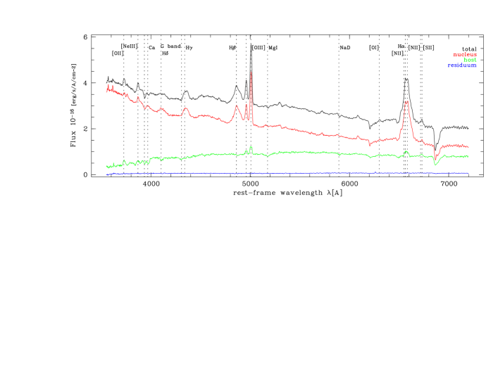
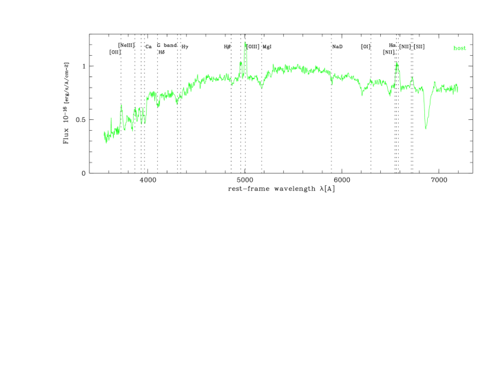
Figure 6: Modelling result EFOSC sample: HE 0952–1552. Shown are, in the top panel, extracted spectrum of the total QSO (top black line), nucleus (red line), host after subtraction of the nuclear model (green line) and residual after subtraction of nucleus and host model (blue). The bottom panel shows the host spectrum alone. Positions of major emission/absorption lines are marked. Given is the rest-frame wavelength. For presentation the spectra have been slightly smoothed to enhance the visibility of spectral features.

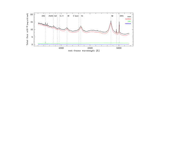
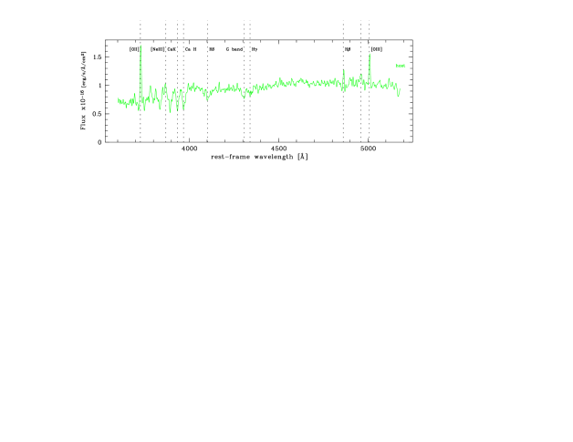
Figure 7: Modelling result FORS sample: HE 1503+0228. Lines as in Figure 6.

6.3 EFOSC example: HE 0952–1552

In the resulting host galaxy spectrum of HE 0952–1552 (Fig. 6) several stellar absorption lines are visible, Ca H and K, G band, Mg I, Na D, and Balmer absorption in H$\beta$ to H$\delta$. The 4000 Å break is prominent. Emission lines from the ISM are also present: [O II] 3727 Å, the [O III] doublet 4959/5007 Å, [N II] 6548/6583 Å and narrow H$\alpha$ also in emission, although the three components are not clearly resolved. The [S II] 6716/6731 Å doublet is also visible and it, too, is blended.

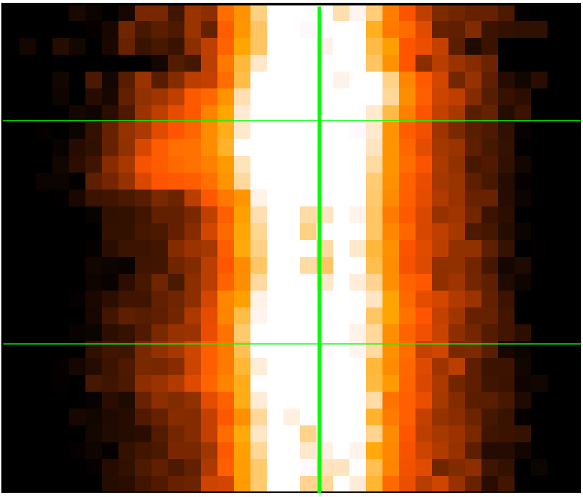
Figure 8: HE 0952–1552: Region of the [O III] emission line doublet at 4959/5007 Å, wavelength increasing from bottom top. The vertical and horizontal lines mark the spatial and spectral centers of the lines. Visible is the effect of rotation and a prominent asymmetric component on the approaching sides of the two lines.

The 2d residuals show significant structure on a level of 10% of the host count rate, or $<2\%$ of the count rate of the input QSO spectrum. In the [O III] 5007 Å component there are clear systematic velocity differences visible between the two sides of the galaxy. A velocity difference between the two sides of the galaxy along the slit can be estimated, though the [O III] emission seems to be spatially asymmetric (Fig. 8). Averaging between 1$\aas@@fstack{\prime\prime}$5 and 3$\aas@@fstack{\prime\prime}$5 radius the two components yields a line of sight velocity difference of $\sim$350 km/s, not deprojected for slit angle orientation and inclination.

Rotation in the absorption lines is also visible. Ca K shows a shift of 5.2 Å between 1$\aas@@fstack{\prime\prime}$5 and 3$\aas@@fstack{\prime\prime}$5 radius of the left and right side, corresponding to an observed rotation velocity of 200 km/s, substantially smaller than the [O III] velocities. In conjunction with the asymmetry of the [O III] line this poses the possibility that one side of the galaxy shows an outflow superposed of ionized gas on the rotation pattern defined by the stars.

The inclination is difficult to assess because of the supposed presence of a significant bulge. From its axial ratio we estimate an inclination of $\sim$50^∘, which would be a lower limit in the presence of a bulge. In general, quasar host galaxies rarely show inclinations above 60^∘ due to the obscuration of the central source beyond that (McLeod & Rieke, 1995; Taylor et al., 1996).

For this range of values, the deprojection factor for the velocity lies between 1.15 and 1.75, depending on the angle between slit and rotational axis of the galaxy (estimated to 0–30^∘), the latter dominating the uncertainty in this case. This leads to a deprojected velocity difference of 230–350 km/s; the best guess is $\sim$280 km/s. This value is consistent with the rotational velocity expected for a massive bulged spiral galaxy as HE 0952–1552.

The rotation seen in the emission lines clearly identifies them as gas emission and not artefacts of the separation. It is more difficult to judge whether the strength of the emission lines determined is correct, or if numerical flux transfer has happened from the nucleus to the host. Due to the low resolution it is not possible to apply a single sided modelling to the lines in this case. The model for the [O II] line shows a somewhat disturbed spectral geometry, with a small dip in the center, while the (much stronger) [O III] lines appear completely undisturbed. Close to the nominal position of the latter appears absorption, compatible with the Balmer absorption in H$\gamma$ and H$\delta$. But it is shifted by 12 Å, which is not due to errors in calibration. H$\alpha$ and the [N II] doublet are blended. In the host spectrum a dip is visible at the nominal H$\alpha$ position. This is also compatible with superposed gas emission and stellar absorption.

6.4 FORS example: HE 1503+0228

HE 1503+0228 is a QSO at redshift $z=0.1350$, with a prominent disk-dominated host with a scale length of 1$\aas@@fstack{\prime\prime}$9. It shows a continuum nucleus-to-host flux ratio of 7–10 integrated over the 1″slit. With these properties it is among the object in the FORS sample that can be studied the easiest. QSOs with more compact host galaxies will be more difficult to separate with larger uncertainties or requiring a better knowledge of the host’s morphology.

Several prominent gas lines are visible in the resulting host galaxy spectrum, in Figure 7. In the $B$ grism [O II], [O III], H$\beta$, Ca H and K and Fe I 5270 are separately modelled with single sided fits. A slight offset between absolute fluxes exists in the overlap regions of $B$ and $R$ grism, of the order of 10% at 5100 Å.

The detected gas emission shows clear signs of rotation, so do the stellar absorption features. The Ca H and K, G band absorption lines are prominent in the $B$ grism.

The full FORS dataset (20 objects) and among it HE 1503+0228 have separately been analysed using the deconvolution method by Courbin et al. (2000). Results have been published in Courbin et al. (2002) and Letawe et al. (2006). In Figure 9 we show the ratio of extracted host galaxy spectra from deconvolution and modelling decomposition in the $B$ grism for HE 1503+0228. The two methods are consistent within about 10% over the higher S/N part of the data above 4000Å. Below 4000Å (rest-frame) the S/N drops and some spikes in difference appear. However, these spikes are not coincident with emission or absorption lines. E.g. at 5007Å no particular difference exists, showing that emission lines are treated consistently between the two methods. The difference of 10% can have different sources. One of them is a sensitivity of the described modelling decomposition to the input host galaxy model. If this is not constrained well enough, a general flux transfer can occur. We have made tests with a $\sim$30% larger host galaxy size, resulting in 20% higher flux values for the host spectrum.

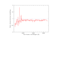
Figure 9: Ratio of derived spectra for the host of HE 1503+0228 from deconvolution and th modelling decomposition described here. The two methods are consistent to about 10% over the higher S/N part of the data. Below 4000Å(rest-frame) the S/N drops and some spikes in difference appear. These are not coincident with emission or absorption lines.

We can also compare line properties, e.g. derived line shifts. When coadding all accessible emission lines we can compute a rotation curve, with a measured maximum velocity of $\sim$160 km/s. Courbin et al. (2002) find very similar values. While deconvolution by Courbin et al. seems to be able to trace the full increase of velocities outside of a few 100 kpc (the innermost pixel), we only resolve the velocity field starting at a radius of $\sim$2 pixels and miss the rise.

Derived line properties are always very consistent between the two methods for all objects in the overlapping sample (see also Table 2). However, derived absolute fluxes of the host galaxy can differ. For HE 1503+0228 this is below 20% and consistent for all wavelengths, this can be stronger in other cases. A detailed quality of fit analysis (Sec. 5.5) is in each case a prerequisite to judge if a separation was successful or failed.

7 Science results

So far we described the decomposition method and did quality checks. We now also want to summarize science results on the two samples. For the FORS sample we will restrict the description to avoid duplicating results that has already been reported in more detail in Letawe et al. (2004, 2006) or Courbin et al. (2002). The results from our two methods are sufficiently similar – whereever we performed the same analysis we agree within our determined error bars. For this reason the emphasis here will lie on i) stellar population fits to the host galaxy continuum, and its comparison to broad band photometry, ii) on peculiar velocities for the EFOSC sample, and iii) on spatial ionized ISM distribution for the FORS sample.

As mentioned, in Table 1 a summary of object properties of the samples is shown, with redshifts, magnitudes, nucleus to host ratio, morphological type and scale length.

Table 1: Objects in the EFOSC (top) and FORS samples (bottom). Listed are redshift $z$, apparent optical magnitude (extinction corrected; $V$ for EFOSC, $B$ for FORS), and in the near-infrared, $H$, nucleus-to-host flux ratio n/h($H$), morphological type of the host ((E)lliptical or (D)isk dominated; ED describes objects fit better with an spheroidal model, but a significant disk contribution can not be ruled out, DE vice versa), and scale length $r_{1/2}$ used in modelling. HE 1201–2409 has a very compact early type host galaxy. It was modelled also with a disk, which allows a better convergence of the fit. In this way at least some of the external spatial information is used. Except for HE 1029–1401 and HE 1434–1600, which are part of the multicolour sample investigated in Jahnke et al. (2004a), the morphological properties are results from Kuhlbrodt (2003) or from Wisotzki et al., in prep.

Object	$z$	$B$,$V$	$H$	n/h ($H$)	Type	$r_{1/2}$ [′′]
HE 0952–1552	0.108	15.8	13.4	0.6	D	2.55
HE 1029–1401	0.085	13.7	12.2	2.1	E	1.95
HE 1201–2409	0.137	16.3	14.2	0.7	E	0.47
					D	3.1
HE 1239–2426	0.082	15.6	12.8	0.9	D	4.4
HE 1310–1051	0.034	14.9	12.7	1.2	D	3.7
HE 1315–1028	0.098	16.8	14.2	0.9	D	3.3
HE 1335–0847	0.080	16.3	14.1	0.45	E	2.4
HE 1416–1256	0.129	16.4	14.4	1.1	E	2.1
HE 0914–0031	0.322	16.0	15.0	3.5	D	2.0
HE 0956–0720	0.3259	16.3	14.3	3.0	D	3.0
HE 1009–0702	0.2710	16.4	14.3	1.8	ED	0.55
HE 1015–1618	0.2475	15.4	13.6	6.0	D	2.2
HE 1029–1401	0.0859	13.3	12.2	2.1	E	1.45
HE 1228+0131	0.117	14.7	12.9	5.4	DE	1.65
PKS 1302–1017	0.2784	14.6	13.6	1.7	E	0.6
HE 1434–1600	0.1445	15.1	13.6	1.2	E	2.2
HE 1442–1139	0.2569	16.8	14.6	0.45	D	1.95
HE 1503+0228	0.1350	16.3	13.6	1.5	D	2.2

7.1 Stellar populations and broadband colours

Stellar populations can either be investigated by analysing diagnostic absorption line ratios, as has been done by Letawe et al. (2006) for the FORS sample. Or, in a more crude way, by fitting stellar population models to the stellar continuum, including characteristic features as the Balmer break around 4000Å. We want to do the latter, to extract stellar age information in comparison to Letawe et al. (2006).

In this process we start by testing the absolute spectrophotometric calibration of the data and precision of our decomposition algorith by comparing the spectra to broad-band fluxes derived in (Jahnke et al., 2004a) for the EFOSC sample. We convert the magnitudes in the $B$, $V$, $R$, and $i$ band to fluxes using the appropriate filter curves and zero points. They are shown as solid symbols in Fig. 10 overplotted over the host galaxy spectra for four objects. By using a slight extrapolation of the spectrum to the red by a stellar population model (see below) $V$, $R$, and $i$ are in very good aggreement with the spectra.

For two objects this is also true for the $B$ band, it is missing for HE 1315–1028, and for HE 1310–1051 $B$ it is off by a factor of 1.5. We have no explanation for this. The $B$ band image for HE 1310–1051 is of very good quality, therefore the decomposition did not have large uncertainties. An apparent asymmetry in the host galaxy, with potentially bluer colours due to enhanced star formation after a merger was masked in the photometry and should not boost the $B$ band flux over the spectrum flux, even if the slit has missed this region. A fit to the optical and NIR colours of this host galaxy suggests a higher fraction of a younger stellar population than the spectrum. We take this as a hint that there might be an underestimation of the blue part of the host galaxy spectrum in this case.

For both samples we we compare the host galaxy spectra to theoretical evolution synthesis models, making use of the GALAXEV model family by Bruzual & Charlot (2003). Used are models based on the Scalo IMF and of solar metallicity. We used a grid of simple single stellar population (SSP) models of different ages, from 0.01 to 14 Gyr, plus a continuous star formation (CSF) model with constant star formation rate for 14 Gyr, created from the SSP models. To this grid we added two SSP composite spectra. No internal dust extinction in the galaxy was added.

We did not perform a rigorous fit but tried to reproduce the spectral slope as well as the absorption line strengths as good as possible with these simplistic models. There are four sources each from the two samples where we trust the decomposition to a degree that we attempt a fit to the overall SED (Figures 10 and 11).

In the EFOSC sample (Fig. 10) two models are roughly matched by single stellar populations of 2 Gyr (HE 1201–2409) and 4 Gyr (HE 1315–1028), however, for the latter the 4000Å-break is slightly smaller in the data than in the model, so it might be slightly younger. These luminosity weighted ages are interesting. While for HE 1315–1028 the age of $\la$4 Gyr is rather typical, for the host is classified as disk dominated (Jahnke et al., 2004a), however HE 1201–2409 was classified as a very compact early type host galaxy, which would point to an excess of young stars from recent star formation. From optical and near-infrared broad-band imaging we found an age matching this result (1–2 Gyr).

The two other QSOs with EFOSC data can not be modelled with single stellar populations. For HE 0952–1552 we find that a combination of a stellar population that is comparably old for a disk-dominated galaxy (5 Gyr) plus a 2.5% contribution from a moderately young population (350 Myr) would work best. The strength of the 4000Å-break is slightly overestimated, pointing to even more young stars, and there is a slight mismatch at 4500 and 5500Å. However, the overall spectral slope is matched quite well.

HE 1310–1051 requires only about 1% of e.g. a 100 Myr population on top of a very evolved population (14 Gyr). Here the 4000Å-break is matched very well. In total this could point to a quite old bulk of stars, with some recent or ongoing star formation, while the morphological analysis classifies the host as disk dominated. Broad band colour also favour a rather old average stellar age of 6 Gyr, although the amount of young stars is higher due to the leverage of the high $B$ band flux point.

In the FORS sample (Fig. 11) HE 1009–0702 is overall rather young, with a mean stellar age of 0.7–1 Gyr, however the morphology is ambiguous, suggesting a bulge plus disk (Tab. 1). Even younger is the extreme case of PKS 1302–1017, the only radio-loud quasar in the sample. It has an elliptical host galaxy (Bahcall et al., 1997) as judged from HST imaging, but there are indications for substantial deviation from a smooth profile in ground based NIR imaging (Kuhlbrodt, 2003). The extracted spectra deviate in the blue somewhat between our decomposition and the deconvolution in Letawe et al. (2006), but the spectrum is consistently very blue, with an extremely young stellar age. There are almost no discernable stellar absorption lines, with only a slight CaK line, weak MgI and absent NaD. This can not be artifacts of the decomposition since no broad emission components of H$\alpha$ and H$\beta$ are visible in the extracted host spectrum.

HE 1442–1139 and HE 1503+0228 are less surprising, being both morphologically disk galaxies with very typical spectra. They are both best fitted with continuous star formation models, plus an added 2.5% of a 100 Myr population in the case of HE 1503+0228. Here also the absorption lines are well matched, substantially better than for any EFOSC object.

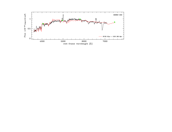
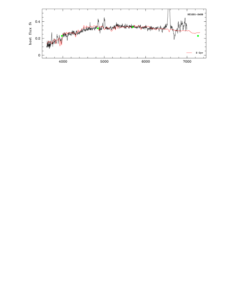
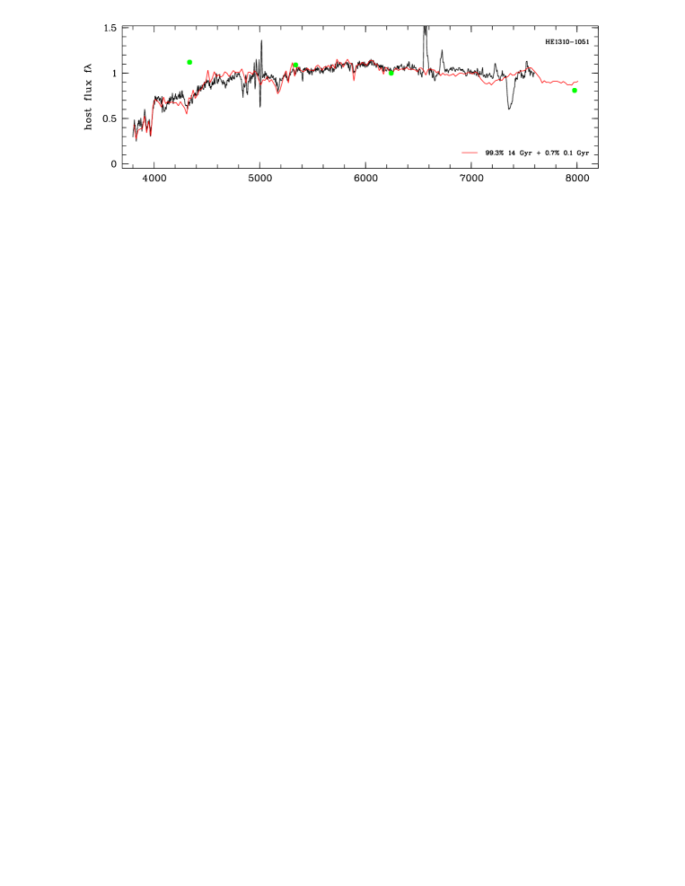
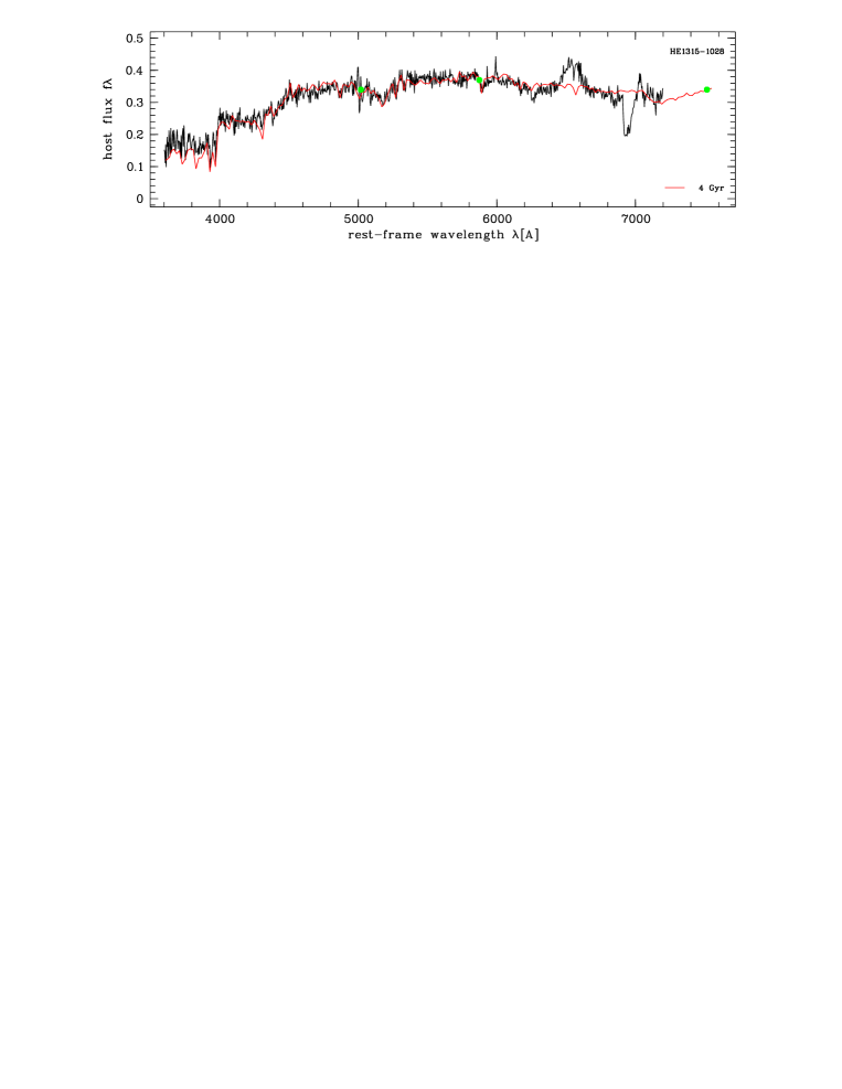
Figure 10: Model fits for four EFOSC objects with sufficient quality. See text for description.

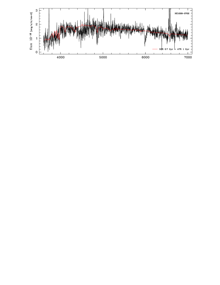
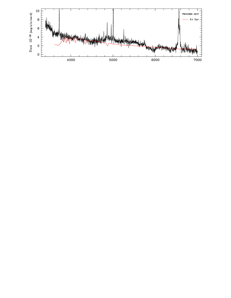
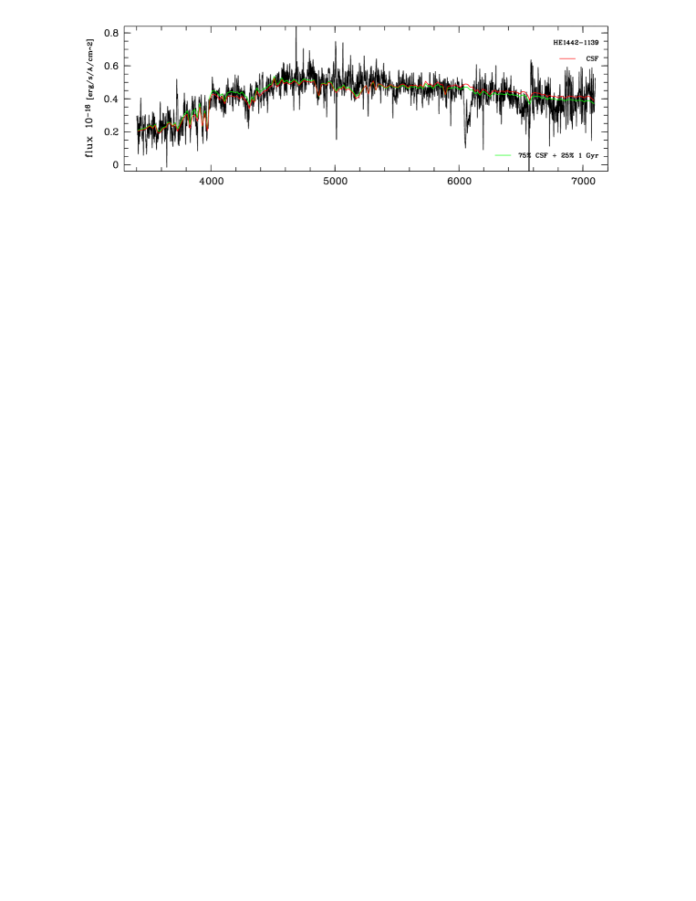
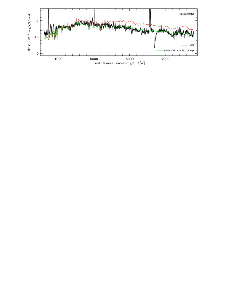
Figure 11: Spectral models for four VLT objects with good quality. See text for description.

7.2 Peculiar velocities

Letawe et al. (2006) find about 50% of the QSO sample to show signs of asymmetries in the hosts or substantial companions near or even inside the host galaxy, which is consistent with the fraction for the EFOSC sample (Jahnke et al., 2004a). In the FORS sample 12/20 hosts have sufficient S/N to determine spatially resolved velocity information, and in six of these cases the velocity fields are consistent with proper rotation curves. The remaining six cases show either very little peculiar velocities (PKS 1302–1017), or show strong signs of interactions, with measured velocities (one side versus systematic velocity) of up to several 100 km/s. The peculiar velocities for the FORS sample are all consistent with the values found by Letawe et al. (2006).

In the EFOSC sample, data quality only permits to extract velocity information for five of the eight objects in the sample – we have stated the measurements for HE 0952–1552 already in Section 6.3. While for the FORS sample normally full rotation curves can be extracted, here the S/N is not large enough to determine more than one velocity value for each side of the host galaxy. Table 2 summarizes the measured and deprojected velocities for both samples.

Table 2: Geometrical, velocity, and stellar population properties of the EFOSC sample. The columns list morphological type (as in Table 1), inclination $i$, angle between slit and major axis $\phi$, detection of rotation in gas emission lines, maximum velocities of the gas as observed ($v_{\mathrm{g,obs}}$) and deprojected ($v_{\mathrm{g,rot}}$), and the same for stellar absorption lines ($v_{\mathrm{s,obs}}$, $v_{\mathrm{s,rot}}$). Velocities are in units of km/s. The last column gives the single-stellar population fit ages from one or two components, “CSF” stands for a continuous star formation model. A “?” is given, if this property is not known, “–” if this property is not accessible. For HE 1315–1028 there are indications for a merging companion in the slit. See text for details.

Object	Type	$i$ [∘]	$\phi$ [∘]	Gas rot.	$v_{\mathrm{g,obs}}$	$v_{\mathrm{g,rot}}$	Stell. rot.	$v_{\mathrm{s,obs}}$	$v_{\mathrm{s,rot}}$	$t_{\mathrm{stellar}}$
HE 0952–1552	D	48	25	y	350	575	y	200	280	97.5% 5 Gyr + 2.5% 350 Myr
HE 1029–1401	E	–	–	y	204	–	n	0	–	–
HE 1201–2409	E	–	–	?	–	–	?	–	–	2 Gyr
HE 1239–2426	D	38	40	?	$<55$	$<140$	?	–	–	–
HE 1310–1051	D	27	10	y	470	$>1000$	?	–	–	99.3% 14 Gyr + 0.7% 100 Myr
HE 1315–1028	D	55	50	?	–	–	y	$\sim$215	610?	4 Gyr
HE 0914–0031	D	–	–	y	180	–	–	–	–	–
HE 1009–0702	E/D	–	–	y	75	–	?	–	–	0.7–1 Gyr
HE 1029–1401	E	–	–	y	180	–	n	0	–	–
PKS 1302–1017	E	–	–	?	$<$40	–	?	–	–	$<$100 Myr
HE 1434–1600	E	–	–	y	140	–	?	–	–	–
HE 1442–1139	D	–	–	y	115	–	y	$\sim$40	–	CSF
HE 1503+0228	D	43	28	y	160	260	y	150	245	97.5% CSF + 2.5% 100 Myr

As noted, for HE 0952–1552 the stellar velocities are consistent with rotation of a massive disk galaxy, while the gas velocities require an additional velocity component. Together with a spatial asymmetry of the emission line (Fig. 8) this is potentially a sign for an outflow.

For HE 1029–1401 the decomposition was not completely successful in the EFOSC data. The SED was unrealistic and much smaller residual are seen in the FORS data (this is the only target common to both datasets). However, around individual absorption and emission lines the decomposition residuals were small, and enough to determine velocities. We measure $\sim$200 km/s rotational velocity in [O III] , consistent with 180 km/s in the FORS data set, and values consistent with zero in the CaK absorption line. So the stellar velocities are consistent with the overall elliptical morphology of the host galaxy, while there is either a disk of gas present in the host, or gas flows in or out from opposite directions with 200 km/s projected velocity. The “rotation curve” from the FORS data is in fact not completely consistent with rotation (rather a curve of constant slope than a classical rotation curve), with either decomposition technique. If not decomposition residuals are responsible for a skewing of the rotation curve, this is a clear sign that the gas motion is dominated by other sources, flows or interaction.

HE 1239–2426 is a ring galaxy, showing a strong ring of stars around a central bulge or bar, the ring inclined by $\sim$40^∘ (asuming intrinsically circular geometry). We find only upper limits in the gas velocities, so either the gas is not moving with more than 140 km/s or the line of sight to the galaxy is in reality more face-on than estimated.

The two remaining host galaxies show peculiarities in their velocities. HE 1310–1051 allows to measure [O III] velocities of 470 km/s. With a fitted inclination of 27^∘ and an angle of 10^∘ between slit and major axis, the deprojected velocity is $>$1000 km/s. Since the geometry of HE 1310–1051 is severely distorted (Jahnke et al., 2004a), both angles have a substantial uncertainty. But even the observed velocity lies outside the limits for disk rotation, so we trace a gas flow outside of a dynamic equilibrium. The absorption lines have too low S/N to be studied.

For HE 1315–1028 on the other hand the stellar absorption lines show signs of peculiar velocities, while the host galaxy’s emission lines are too weak to have velocities measured. The stellar line of sight velocity is $\sim$160 km/s in CaK and $\sim$275 km/s in NaD. The host galaxy has in principle a simple geometry, with inclination of 50–60^∘ and a slit angle of $\sim$50^∘. With these angles the projection is a factor of 2.8, which would translate into a deprojected velocity of 610 km/s, clearly too much for normal disk rotation. Since it seems unlikely that the inclination and major axis positions are so far off to in fact reach a physically sensible deprojected velocity, it is possible that we measure the velocity of a merging companion. HE 1315–1028 has a companion within its disk (in projection?) that is covered by the slit. It is conceivable that this companion is moving towards HE 1315–1028 at a velocity comparible to the rotation velocity of HE 1315–1028, creating the projected velocity without stellar rotation of this velocity.

7.3 Spatial distribution of the ionized ISM

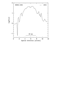
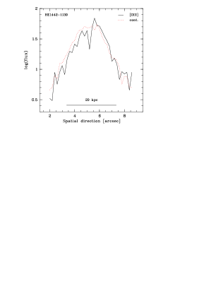
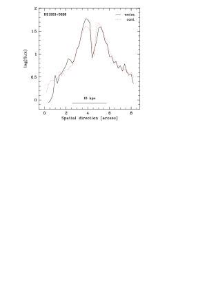
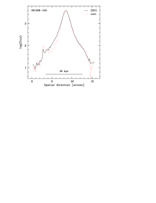
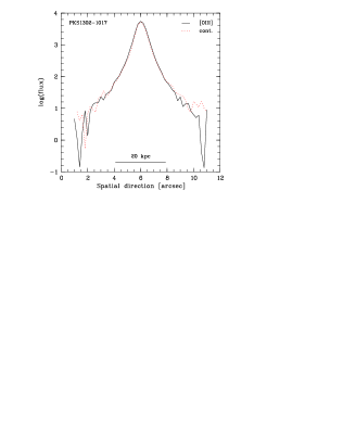
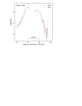
Figure 12: Radial surface brightness profiles of the [O III] 5007 Å emission line and adjacent continuum. The solid curve is the emission line, the dashed red curve the continuum, scaled to match the emission in flux. For HE 1503+0228 all emission lines in the $B$ grism were coadded.

In the host galaxy spectra the spatial information from the slits is still available. After separation and special treatment of the narrow emission lines from the host galaxies (see Section 5.3) it is not only possible to measure line ratios to determine ionisation properties of the ISM as a whole, but also the spatial distribution of line emission can be compared to the stellar continuum emission. This can be complementary to an analysis of peculiar velocities to search for signs of irregularities.

In case that the ionising radiation reaches the outer limits of the host, and the ionising spectrum does not change, the radial profile of an emission line simply maps the distribution of the ISM. Thus if an emission line can be continuously traced out to the noise level, and if this coincides with the traceability of the continuum, then this is suggestive of ionisation throughout the galaxy. If the profiles also coincide, the distribution of stars and ISM is very similar (on the scales samples). If, however, at some radius the profile ends, one of two causes are possible. Either a limited extention of the gas, or, if the nucleus or a circumnuclear starburst were the source for ionised gas, and the number of high energy photons were limited so that only inside a given radius the gas was ionised.

We show the logarithmic radial emission profiles of [O III]  for 6 objects from the FORS sample in Figure 12. They were produced as variance weighed averages of the spatial profile of [O III]  (both components added), subtracting the underlying continuum and compare it to the shape of the adjacent continuum itself. For HE 1503+0228 we coadded all available lines in the $B$ grism. For HE 0914–0031 no continuum can be extracted, because this is not resolved. We ordered the objects by morphology as determined from imaging in Jahnke et al. (2004a), with three disks in the top row, the spheroidal dominated hosts in the bottom.

The disks more or less conform with the exponential disk profile, which would appear as a straight line in the log diagram, modified by the seeing: HE 0914–0031 shows no cutoff or deviation from a pure exponential disk profile. For HE 1442–1139 continuum and line emission are consistent, if one accounts for a slight shift in centers introduced by a sky line residual. The profiles of HE 1503+0228 are disturbed in the centre as a result of modelling. While for the very centre the profiles are oversubtracted, they show an excess at around 1$\aas@@fstack{\prime\prime}$5 distance from the center, creating an inflection further out. This is a signature of the residuals of the nuclear model, not a sign for a spheroidal host. Line and continuum are compatible.

While PKS 1302–1017 shows two very similar profiles, supporting the case of no rotational velocity field detected in the line emission (see Letawe et al., 2006), the two other spheroid dominated early type hosts are more interesting.

For HE 1029–1401 peculiar gas motion is detected consistent with rotation of 150–200 km/s, despite that we find a clear spheroidal morphology and no trace of rotational velocities the stellar absorption lines. The right hand side of the line profile coincides with the profile of the continuum. While the central part reflects the PSF-broadened emision from the narrow-line-region of the AGN, the line emission on the left hand side significantly deviates from the continuum emission. Outside of a few kpc from the centre (outside the inflection points) the line emission is very similar to an exponential disk profile, while between 1 and 5 kpc distance from the centre the continuum emission clearly is not (the secondary peak at 3$\aas@@fstack{\prime\prime}$5 is due to structure in the CCD and flatfielding and visible for all of the spectrum). This gives further support to the notion that the velocity seen for the ISM is actually rotational in nature and not an outflow. HE 1029–1401 has likely a low mass stellar and gas disk that can only be seen in very deep imaging, but that shows up in the bright emission lines.

HE 1434–1600 is a very interesting case and has extensively been described in Letawe et al. (2004). In the spectrum, the central pixels are disturbed by modeling residuals. When scaling the continuum so that the outer parts of the two profiles coincide, an excess of line emission can be seen further in, i.e., the gas emission surface brightness drops faster with increasing radius than the continuum emission. In addition, the emission decreases again in the central part, so that close to the nucleus the line emission is less than further out (this result is not affected by modelling residuals, see also Letawe et al., 2004). While the nucleus is clearly the source of ionising radiation as judged from emission line rations, the gas does not extend all through the galaxy but is depleted in the centre, the system is not relaxed – consistent with the result by Letawe et al. (2004) that HE 1434–1600 is a potential post merging system.

This drop in [O III] , might also be present in the stellar continuum, but is at least substantially weaker. The quality of the separation process is not sufficient to resolve this. However, the turnover is actually also the likely source for the modelling residuals: The model assumption of a smoothly decreasing galaxy profile is violated, thus both host and nuclear model are somewhat mismatched. This then is the result of the turnover, not its cause. What remains to be resolved is if the velocities and gas depletion are the result of the system merging with its nearest companion, if the AGN is blowing out gas on a kiloparsec scale, or if the gas is following a coordinated rotation in a disk around the bulge.

8 Discussion and summary

As we have shown, separating host galaxy and nuclear emission in on-nucleus spectra is possible. This works not only for low luminosity Seyfert nuclei, but also for nuclei substantially brighter than their host when integrated over the area of the slit. The limiting factor in the success and quality of the separation is clearly the quality of fixing the spatial light distributions of the components, i.e. the error in determining the PSF and the morphology of the host. A strong advantage, for higher nucleus–host contrasts even a requirement, is the incorporation of external information on the host galaxy’s morphology from (comparably) cheap imaging data.

We have shown for three cases that broad band host galaxy fluxes are reliably matched, showing that even spectrophotometric measurements can be performed under good conditions. Deconvolving the spatial domain at each wavelength numerically as done in Courbin et al. (2000) delivers a very similar results, to consistently $<$10% difference to our approach, while applying a completely complementary approach. As a difference to the spectral eigenvector decomposition technique described by Vanden Berk et al. (2006) – yet again complementary – both these methods retain the two-dimensional information of the spectrum, allowing an analysis of spatial structure.

Any of the two decomposition/deconvolution methods is difficult to calibrate against the influence of PSF uncertainties or S/N issues by itself. Below a certain S/N both methods will break down, the exact point depending on the precision of PSF determination and the algorithmic details. While in the high S/N regime both methods work without large differences and errors, it is very valuable to actually have two completely independent methods that can both be applied in lower S/N cases to cross-check the results. Since lower S/N data are i) less expensive and easier to obtain, and ii) the only option for higher redshifts, having two independent decomposition techniques is extremely valuable.

Scientifically, both investigated samples show similar characteristics, which is not surprising, as their selection functions, redshifts, and magnitudes are similar. In both the FORS and EFOSC samples, about 50% of the sources show signs of deviation from a symmetric and undisturbed morphology, as judged from their images (Kuhlbrodt, 2003; Jahnke et al., 2004a), pointing to recent or ongoing events of interaction or merging with neighbors. Both samples have QSOs with bulge or disk dominated host galaxies, and for both samples luminosity weighted stellar ages are found fot most galaxies. While these are consistent with optical morphology for the disk dominated hosts, these are unusual for the bulge dominated ones. Aside from PKS 1302–1017 these stellar populations, however, do not appear to be general starburst populations, but mixes of old and young population, or, if expressed as a single age, 1–2 Gyr of age. This is typical rather for intermediate to late type spirals, in clear contradiction to the observed morphology, if these were normal, average field galaxies.

Interestingly enough, there are signs for systematic gas velocities found in both samples, not only in the disk dominated hosts, but also in the bulge dominated. On the other hand it is not clear, whether the source for this is simple disk rotation, e.g. that HE 1029–1401 and HE 1434–1600 are not consisting solely of a spheroid component, but have a comparably low luminosity stellar and gas disk as well. However, the velocity fields of the two systems just mentioned show deviations from a simple disk rotation (Letawe et al., 2004, 2006) law, which could also allow the interpretation that these might be signs of in- or outflows of ISM gas.

The connection of a substantial distortion rate, signs for recent star formation and AGN activity is very suggestive and the earlier conclusions from imaging (Jahnke et al., 2004a) are reinforced by the presented spectra. Comparing broad band colours and host galaxy spectra to synthetic models both point, in connection with distorted velocity fields, to a interaction–AGN connection acting on these galaxies.

In the light of scenarios of AGN feedback (e.g., Hopkins et al., 2006) as a crucial factor in the creation of the blue cloud and red sequence bimodality in galaxy colour-magnitude diagrams, there are two questions to our datasets: First, do we see merging in connection with every bright quasar? Here the answer is no, not with the current data. There are several objects that have no discernable close companions or even signs of ongoing merger. Several of our sample objects are seemingly undistorted disk galaxies. However, seeing merger signs is an issue of spatial resolution. Recently Canalizo et al. (in prep) reobserved early type quasar host galaxies from the samples by Dunlop et al. (2003), now with five orbits of HST ACS time each, instead of one orbit of WFPC2. While these hosts looked smooth and symmetric before in shallow data, they now show shells and whisps that mark these as merger remnants.

The second question is, if we find traces for outflows, powered by the AGN, that will eventially evacuate the host galaxy of any ISM to truncate star formation. We see line emission, so signs of gas, in almost all hosts. Sometimes ionized by the nuclear spectrum, in the other half of the cases by hot stars. Interesting is the drop in emission line intensity in the centre of HE 1434–1600, combined with a velocity field that suggests deviations from a normal Keplerian rotation. These can be counted as signs of interaction, but if the ISM in the central part of the galaxy has been blown out is difficult to support – the data is more pointing towards interaction than AGN feedback.

Since also none of the other objects shows large-scale signs of outflows, but either Keplerian rotation curves or coherent morphological and velocity field distortions, we see no indications for large scale flows in these data. If the evacuation of the galaxies’ ISM is quenching the QSO activity very shortly after the blowout, this result is in accordance with the model, since these black holes are still strongly accreting. A connection of substantial merging and AGN activity, however, is supported for about half of the objects.

References

- Abraham et al. (1992) Abraham R. G., Crawford C. S., McHardy I. M., 1992, ApJ, 401, 474
- Bahcall et al. (1997) Bahcall J. N., Kirhakos S., Saxe D. H., Schneider D. P., 1997, ApJ, 479, 642
- Boroson & Oke (1982) Boroson T. A., Oke J. B., 1982, Nature, 296, 397
- Boroson & Oke (1984) Boroson T. A., Oke J. B., 1984, ApJ, 281, 535
- Boroson et al. (1982) Boroson T. A., Oke J. B., Green R. F., 1982, ApJ, 263, 32
- Boroson et al. (1985) Boroson T. A., Persson S. E., Oke J. B., 1985, ApJ, 293, 120
- Bruzual & Charlot (2003) Bruzual G., Charlot S., 2003, MNRAS, 344, 1000
- Canalizo & Stockton (2000) Canalizo G., Stockton A., 2000, ApJ, 528, 201
- Courbin et al. (2002) Courbin F., Letawe G., Magain P., Wisotzki L., Jablonka P., Jahnke K., Kuhlbrodt B., Alloin D., Meylan G., Minniti D., Burud L., 2002, A&A, 394, 863
- Courbin et al. (2000) Courbin F., Magain P., Kirkove M., Sohy S., 2000, ApJ, 529, 1136
- Dong et al. (2005) Dong X.-B., Zhou H.-Y., Wang T.-G., Wang J.-X., Li C., Zhou Y.-Y., 2005, ApJ, 620, 629
- Dunlop et al. (2003) Dunlop J. S., McLure R. J., Kukula M. J., Baum S. A., O’Dea C. P., Hughes D. H., 2003, MNRAS, 340, 1095
- Dunlop et al. (1993) Dunlop J. S., Taylor G. L., Hughes D. H., Robson E. I., 1993, MNRAS, 264, 455
- Ferrarese & Merrit (2000) Ferrarese L., Merrit D., 2000, ApJ, 539, L9
- Floyd et al. (2004) Floyd D. J. E., Kukula M. J., Dunlop J. S., McLure R. J., Miller L., Percival W. J., Baum S. A., O’Dea C. P., 2004, MNRAS, 355, 196
- Green et al. (1978) Green R. F., Williams T. B., Morton D. C., 1978, ApJ, 226, 729
- Hao et al. (2005) Hao L., Strauss M. A., Tremonti C. A., Schlegel D. J., Heckman T. M., Kauffmann G., Blanton M. R., Fan X., Gunn J. E., Hall P. B., Ivezić Ž., Knapp G. R., Krolik J. H., Lupton R. H., Richards G. T., Schneider D. P., Strateva I. V., Zakamska N. L., Brinkmann J., Brunner R. J., Szokoly G. P., 2005, AJ, 129, 1783
- Hickson & Hutchings (1987) Hickson P., Hutchings J. B., 1987, ApJ, 312, 518
- Hopkins et al. (2006) Hopkins P. F., Hernquist L., Cox T. J., Di Matteo T., Robertson B., Springel V., 2006, ApJS, 163, 1
- Horne (1986) Horne K., 1986, PASP, 98, 609
- Hughes et al. (2000) Hughes D. H., Kukula M. J., Dunlop J. S., Boroson T., 2000, MNRAS, 316, 204
- Hutchings & Crampton (1990) Hutchings J. B., Crampton D., 1990, AJ, 99, 37
- Hutchings & Hickson (1988) Hutchings J. B., Hickson P., 1988, AJ, 95, 1363
- Jahnke et al. (2006) Jahnke K., et al., 2007, in prep
- Jahnke et al. (2004a) Jahnke K., Kuhlbrodt B., Wisotzki L., 2004a, MNRAS, 352, 399
- Jahnke et al. (2004b) Jahnke K., Sánchez S. F., Wisotzki L., Barden M., Beckwith S. V. W., Bell E. F., Borch A., Caldwell J. A. R., Häußler B., Heymans C., Jogee S., McIntosh D. H., Meisenheimer K., Peng C. Y., Rix H.-W., Somerville R. S., Wolf C., 2004b, ApJ, 614, 568
- Kauffmann et al. (2003) Kauffmann G., Heckman T. M., Tremonti C., Brinchmann J., Charlot S., White S. D. M., Ridgway S., Brinkmann J., Fukugita M., Hall P., Ivezic Z., Richards G., Schneider D., 2003, MNRAS, 346, 1055
- Kuhlbrodt (2003) Kuhlbrodt B., 2003, PhD thesis, University of Hamburg, http://www.sub.uni-hamburg.de/disse/1036/dissertation.pdf
- Kuhlbrodt et al. (2004) Kuhlbrodt B., Wisotzki L., Jahnke K., 2004, MNRAS, 349, 1027
- Letawe et al. (2004) Letawe G., Courbin F., Magain P., Hilker M., Jablonka P., Jahnke K., Wisotzki L., 2004, A&A, 424, 455
- Letawe et al. (2006) Letawe G., Magain P., Courbin F., Jablonka P., Jahnke K., G. M., Wisotzki L., 2007, submitted to MNRAS, astro-ph/0605288
- MacKenty & Stockton (1984) MacKenty J. W., Stockton A., 1984, ApJ, 283, 64
- McLeod & Rieke (1995) McLeod K. K., Rieke G. H., 1995, ApJ, 441, 96
- Magain et al. (1998) Magain P., Courbin F., Sohy S., 1998, ApJ, 494, 472
- Magain et al. (2005) Magain P., Letawe G., Courbin F., Jablonka P., Jahnke K., Meylan G., Wisotzki L., 2005, Nature, 437, 381
- Moffat (1969) Moffat A. F. J., 1969, A&A, 3, 455
- Morton et al. (1978) Morton D. C., Williams T. B., Green R. F., 1978, ApJ, 219, 381
- Nolan et al. (2001) Nolan L. A., Dunlop J. S., Kukula M. J., Hughes D. H., Boroson T., Jimenez R., 2001, MNRAS, 323, 308
- Peng et al. (2002) Peng C. Y., Ho L. C., Impey C. D., Rix H.-W., 2002, AJ, 124, 266
- Press et al. (1995) Press W. H., Teukolsky S. A., Vetterling W. T., Flannery B. P., 1995, Numerical recipes in C, 2nd edn. Cambridge University Press
- Richstone & Oke (1977) Richstone D. O., Oke J. B., 1977, ApJ, 213, 8
- Saglia et al. (1993) Saglia R. P., Bertschinger E., Baggley G., Burstein D., Colless M., Davies R. L., McMahan Jr. R. K., G. W., 1993, MNRAS, 264, 961
- Sánchez et al. (2006) Sánchez S. F., García-Lorenzo B., Jahnke K., Mediavilla E., González-Serrano J. I., Christensen L., Wisotzki L., 2006, AN, 327, 167
- Sánchez et al. (2004) Sánchez S. F., Jahnke K., Wisotzki L., Barden M., Beckwith S. V. W., Bell E. F., Borch A., Caldwell J. A. R., Häußler B., Heymans C., Jogee S., McIntosh D. H., Meisenheimer K., Peng C. Y., Rix H.-W., Somerville R. S., Wolf C., 2004, ApJ, 614, 586
- Stockton (1976) Stockton A., 1976, ApJ, 205, L113
- Taylor et al. (1996) Taylor G. L., Dunlop J. S., Hughes D. H., Robson E. I., 1996, MNRAS, 283, 930
- Trujillo et al. (2001) Trujillo I., Aguerri J. A., Cepa J., Gutiérrez C. M., 2001, MNRAS, 328, 977
- Vanden Berk et al. (2006) Vanden Berk D. E., Shen J., Yip C.-W., Schneider D. P., Connolly A. J., Burton R. E., Jester S., Hall P. B., Szalay A. S., Brinkmann J., 2006, AJ, 131, 84
- Wampler et al. (1975) Wampler E. J., Burbidge E. M., Baldwin J. A., Robinson L. B., 1975, ApJ, 198, L49
- Wyckoff et al. (1980) Wyckoff S., Gehren T., Morton D. C., Albrecht R., Wehinger P. A., Boksenberg A., 1980, ApJ, 242, L59
- Wyckoff et al. (1980) Wyckoff S., Wehinger P. A., Spinrad H., Boksenberg A., 1980, ApJ, 240, 25
- Zakamska et al. (2005) Zakamska N. L., Schmidt G. D., Smith P. S., Strauss M. A., Krolik J. H., Hall P. B., Richards G. T., Schneider D. P., Brinkmann J., Szokoly G. P., 2005, AJ, 129, 1212
- Zakamska et al. (2003) Zakamska N. L., Strauss M. A., Krolik J. H., Collinge M. J., Hall P. B., Hao L., Heckman T. M., Ivezić Ž., Richards G. T., Schlegel D. J., Schneider D. P., Strateva I., Vanden Berk D. E., Anderson S. F., Brinkmann J., 2003, AJ, 126, 2125