Magnetic Helicity and the Relaxation of Fossil Fields

Abstract

In the absence of an active dynamo, purely poloidal magnetic field configurations are unstable to large-scale dynamical perturbations, and decay via reconnection on an Alfvénic timescale. Nevertheless, a number of classes of dynamo-free stars do exhibit significant, long-lived, surface magnetic fields. Numerical simulations suggest that the large-scale poloidal field in these systems is stabilized by a toroidal component of the field in the stellar interior. Using the principle of conservation of total helicity, we develop a variational principle for computing the structure of the magnetic field inside a conducting sphere surrounded by an insulating vacuum. We show that, for a fixed total helicity, the minimum energy state corresponds to a force-free configuration. We find a simple class of axisymmetric solutions, parametrized by angular and radial quantum numbers. However, these solutions have a discontinuity in the toroidal magnetic field at the stellar surface which will exert a toroidal stress on the surface of the star. We then describe two other classes of solutions, the standard spheromak solutions and ones with fixed surface magnetic fields, the latter being relevant for neutron stars with rigid crusts. We discuss the implications of our results for the structure of neutron star magnetic fields, the decay of fields, and the origin of variability and outbursts in magnetars.

1 Introduction

The importance of magnetic helicity has long been appreciated in the context of force-free plasma dynamics (Woltjer, 1958, 1962). This is due primarily to the fact that helicity has been experimentally shown to be conserved during magnetic reconnection (Taylor, 1974; Ji et al., 1995; Heidbrink & Dang, 2000; Hsu & Bellan, 2002), even when a substantial fraction of the magnetic energy has been dissipated.

In the context of stars, numerical magnetohydrodynamics simulations of initially random fields in a conducting sphere reveal that magnetic helicity plays a crucial role in determining the final magnetic configuration (Braithwaite & Spruit, 2004). In particular, after a period of violent reconnection, which occurs on the Alfvén crossing timescale, a stable, mostly dipolar field develops, the strength of which depends solely upon the initial helicity. In the absence of initial helicity, the final magnetic field vanishes. Relevant systems include magnetic A stars, white dwarfs and neutron stars. In the present paper we are interested primarily in neutron stars.

The simplicity of the final solution found by Braithwaite & Spruit (2004) and others (e.g., Yoshida et al., 2006) suggests that a simple analytical model can be developed. We present here a formalism that might be relevant for understanding the nature of the final equilibrium. Our approach is based on a variational approach that encodes the principle of conservation of total helicity, as proposed by Taylor 1974. We do not address the dynamical path that a system will follow starting from its initial state, but simply attempt to construct the final state of the system. Thus, we present a set of magnetic field solutions as a function of the magnetic helicity. We obtain these solutions via a variational energy principle in which the integrated helicity is held fixed.

In §2 we state the variational principle and derive the governing field equations. §3, which is the heart of this paper, then solves the equations under different conditions, assuming axisymmetry, and discusses the long term evolution of the resulting magnetic field. Explicit forms for some illustrative solutions are given in §3.6. §4 discusses the implications of the results and considers possible applications to neutron stars. A number of technical details are given in the Appendices, including a comparison of our approach, which is based on conservation of total helicity, and the approach of citepFiel:86, who considers a conserved microscopic helicity associated with individual magnetic flux tubes.

2 Helicity, Minimum Energy, and the Force-Free Condition

The magnetic helicity density is defined by $h\equiv{\mn@boldsymbol{\rm A}}\cdot{\mn@boldsymbol{\rm B}}$, where ${\mn@boldsymbol{\rm A}}$ is the vector potential and ${\mn@boldsymbol{\rm B}}\equiv{\mn@boldsymbol{\nabla}\times}{\mn@boldsymbol{\rm A}}$ is the magnetic field. Generally, $h$ is gauge dependent. Nevertheless, the volume integrated helicity can be made gauge independent by a suitable choice of integration. That is,

$$H\equiv\int_{V}\frac{1}{8\pi}{\mn@boldsymbol{\rm A}}\cdot{\mn@boldsymbol{\rm B}}\,{{\rm d}^{3}\!x}\,,$$ (1)

is gauge invariant if ${\mn@boldsymbol{\rm B}}\cdot{{\rm d}\mn@boldsymbol{S}}=0$ everywhere on the boundary of $V$. While during reconnection the local helicity density is not conserved, to a good approximation the total helicity is (Taylor, 1974). This experimental fact suggests that the integrated quantity $H$ plays an important role in determining the final magnetic field configuration, and is the foundation of our analysis. In contrast to the helicity, the magnetic energy,

$$U\equiv\int_{V}\frac{1}{8\pi}{\mn@boldsymbol{\rm B}}\cdot{\mn@boldsymbol{\rm B}}\,{{\rm d}^{3}\!x}\,,$$ (2)

is not conserved during reconnection. Indeed, reconnection can convert a substantial fraction of the magnetic energy into thermal energy of the plasma.

In the absence of a dynamo, the equilibrium state of the field will be associated with its minimum energy state. That is, reconnection will proceed until the maximum amount of magnetic energy is converted into heat. If there are no constraints on the system, the entirety of the magnetic energy will be converted. However, even under randomly chosen initial conditions, a non-zero helicity will initially be present, and subsequently must be conserved. Thus, there is a limit to how much magnetic energy can be converted into heat, and the final configuration must consist of a non-vanishing magnetic field. This situation naturally lends itself to a variational approach, which we explore in the following subsections.

In our analysis we seek to minimize the total magnetic energy (2) subject to a fixed value of the total helicity (1). However, before doing this we might ask: Is it correct to minimize only the magnetic energy and to exclude contributions to the energy from the underlying fluid? The answer is yes. In the context of a constrained total helicity, the equations governing the fluid equilibrium, up to a non-radial surface stress (which we will assume is balanced by a rigid crust), are completely separable from those governing the magnetic field structure. (The reader is referred to Appendix A for a discussion of this question and a comparison of our total helicity conservation approach and that of Field (1986) who considered helicity conservation on individual field loops). That is, subject to the constraint of fixed helicity, we might have considered minimizing

$$U_{\rm tot} =\int_{V}\rho\left[\epsilon+\frac{1}{2}\Phi\right]\,{{\rm d}^{3}\!x}+\int_{V}\frac{1}{8\pi}{\mn@boldsymbol{\rm B}}\cdot{\mn@boldsymbol{\rm B}}\,{{\rm d}^{3}\!x}$$ (3)

$$\equiv U_{f}(\rho,V)+U({\mn@boldsymbol{\rm B}},V)\,,$$

where $\epsilon$ and $\Phi$ are the specific internal energy and self-gravitational potential of the fluid, respectively, and we assume for simplicity that the star is barotropic (although this is not necessary). Since the helicity constraint depends upon only the magnetic field, the magnetic and hydrodynamic contributions to the energy are distinct, and thus, for a fixed $V$, may be minimized independently. As a consequence, the equilibrium magnetic field configuration will not explicitly depend upon the hydrostatic structure of the star. Furthermore, such a state will correspond to a global minimum of the combined energy, $U_{\rm tot}$. Perturbations around such a state will necessarily increase $U_{f}$ and $U$, otherwise these would not be independent minima, and thus will increase $U_{\rm tot}$. Here and henceforth, when we refer to “helicity” we mean the total helicity defined in equation (1), as distinct from the local helicity density $h={\mn@boldsymbol{\rm A}}\cdot{\mn@boldsymbol{\rm B}}$ or the helicity associated with a single magnetic loop (Appendix A).

A somewhat subtle point to note is that the fluid and magnetic field structure are implicitly coupled by the definition of $V$, the volume of the conducting region (the star). That $V$ is finite is critical to the existence of a stable magnetic field configuration. Indeed, if $V$ is infinite there can exist no equilibrium magnetic field configuration with non-vanishing ${\mn@boldsymbol{\rm B}}$. This is a result of the fact that $U$ is proportional to $B^{2}$, and hence the field will naturally expand to fill all available space and therefore have vanishing strength. In the case of a star, equilibrium is a consequence of the star’s self-gravity. This enters into the determination of the magnetic field by constraining the size of the conducting region, $V$, which anchors the magnetic field. Generally, $U_{\rm tot}$ must be minimized with respect to $V$ as well as $\rho$ and ${\mn@boldsymbol{\rm B}}$. However, since both $U$ and $U_{f}$ are functions of $V$, the stellar radius, $R$, implicitly couples the structure of the magnetic field and the fluid. We will discuss how this may be done explicitly in §3.3.

Woltjer (1958) demonstrated that, in the context of uniform media, extremizing the magnetic energy subject to a fixed total helicity results in the force-free equation,

$${\mn@boldsymbol{\nabla}\times}{\mn@boldsymbol{\rm B}}=\alpha{\mn@boldsymbol{\rm B}}\,,$$ (4)

where $\alpha$ is a Lagrange multiplier (Appendix B). Such a field configuration is known as a Woltjer state. The situation is more complicated if there are constraints upon the currents that can be driven in the conducting material. The simplest case, and the one of particular interest here, is when the system under consideration can be separated into two distinct regions: an inner region of infinite conductivity (type-I region) which corresponds to the interior of the star, and an outer region of vanishing conductivity (type-II region) which corresponds to the vacuum exterior of the star.

Given two such regions, the standard variational principle for uniform media may be extended by the inclusion of Lagrange multipliers $\alpha$ and ${\mn@boldsymbol{\lambda}}(\mn@boldsymbol{x})$. Thus, we seek to extremize the quantity

$$S=\int_{V}\frac{1}{8\pi}\left({\mn@boldsymbol{\rm B}}\cdot{\mn@boldsymbol{\rm B}}-\alpha{\mn@boldsymbol{\rm A}}\cdot{\mn@boldsymbol{\rm B}}+\frac{8\pi}{c}f{\mn@boldsymbol{\lambda}}\cdot{\mn@boldsymbol{\rm J}}\right){{\rm d}^{3}\!x}\,,$$ (5)

where the current ${\mn@boldsymbol{\rm J}}$ is related to the magnetic field in the normal way, ${\mn@boldsymbol{\rm J}}\equiv c{\mn@boldsymbol{\nabla}\times}{\mn@boldsymbol{\rm B}}/4\pi$, and $f(\mn@boldsymbol{x})$ vanishes in regions of infinite conductivity (type-I region) and is unity otherwise (type-II region). Unlike $\alpha$, which corresponds to fixing $H$ and is a scalar constant, the ${\mn@boldsymbol{\lambda}}$ are vectors and functions of position; the difference arises because of the global versus local nature of their respective constraints.

Varying $S$ with respect to ${\mn@boldsymbol{\rm A}}$, holding $\delta{\mn@boldsymbol{\rm A}}$ fixed on some outer boundary (not on the boundaries between type-I and type-II regions) gives

$${\mn@boldsymbol{\nabla}\times}{\mn@boldsymbol{\rm B}}=\alpha{\mn@boldsymbol{\rm B}}-{\mn@boldsymbol{\nabla}\times}{\mn@boldsymbol{\nabla}\times}f{\mn@boldsymbol{\lambda}}\,,$$ (6)

and varying with respect to $\lambda$ trivially gives

$$f{\mn@boldsymbol{\nabla}\times}{\mn@boldsymbol{\rm B}}=0\,.$$ (7)

Within type-I ($f=0$) regions, equations (6) & (7) reduce identically to the Woltjer force-free condition (4). In contrast, within type-II ($f=1$) regions, the additional terms are required to make equations (6) and (7) consistent with each other. In particular, inserting the latter into the former gives

$$\alpha{\mn@boldsymbol{\rm B}}={\mn@boldsymbol{\nabla}\times}{\mn@boldsymbol{\nabla}\times}{\mn@boldsymbol{\lambda}}\,.$$ (8)

This implies that

$${\mn@boldsymbol{\nabla}\times}{\mn@boldsymbol{\lambda}}=\alpha{\mn@boldsymbol{\rm A}}+\alpha{\mn@boldsymbol{\nabla}}\Lambda$$ (9)

for some $\Lambda$, the explicit form of which depends upon the gauge choices for ${\mn@boldsymbol{\rm A}}$ and ${\mn@boldsymbol{\lambda}}$. A natural gauge for the former is the so-called Force-Free Gauge in which ${\mn@boldsymbol{\rm B}}=\alpha{\mn@boldsymbol{\rm A}}$ (see Appendix B). This happens also to be a Lorentz gauge (i.e., since we are concerned with stationary solutions, ${\mn@boldsymbol{\nabla}\cdot}{\mn@boldsymbol{\rm A}}=0$).

As discussed in detail in Appendix C, the discontinuous nature of $f$ at the boundaries between type-I and type-II regions implies the standard set of boundary conditions:

$${\mn@boldsymbol{\hat{\rm n}}}\cdot\left({\mn@boldsymbol{\rm B}}_{\rm I}-{\mn@boldsymbol{\rm B}}_{\rm II}\right) =0\,,$$ (10)

$${\mn@boldsymbol{\hat{\rm n}}}\times\left({\mn@boldsymbol{\rm B}}_{\rm I}-{\mn@boldsymbol{\rm B}}_{\rm II}\right) =\frac{4\pi}{c}\mn@boldsymbol{K}\,.$$

Generally, for each choice of $\alpha$ and $\Lambda$, a family of solutions which are local minima of magnetic energy subject to the helicity constraint may be produced. The global minimum can then be found by inspection.

In the case of a uniform medium it is possible to show that the magnetic energy and helicity are related by

$$U=\alpha H.$$ (11)

In contrast, for non-uniform media no such simple relation exists. This is because the force-free gauge is not generally a Lorentz gauge in the type-II regions. However, we can parametrize the departure from the uniform-medium expression in terms of the gauge transformation that relates a Lorentz gauge in the type-II regions to that determined by the continuity of ${\mn@boldsymbol{\rm A}}$ at the boundaries.

In particular, let $\varphi$ be the field potential of the magnetic field in type-II regions (i.e., ${\mn@boldsymbol{\rm B}}={\mn@boldsymbol{\nabla}}\varphi$) and $\Lambda_{\rm L}$ be a gauge function which relates ${\mn@boldsymbol{\rm A}}$ to the Lorentz gauge in type-II regions (i.e., ${\mn@boldsymbol{\rm A}}={\mn@boldsymbol{\rm A}}_{\rm L}+{\mn@boldsymbol{\nabla}}\Lambda_{\rm L}$ where ${\mn@boldsymbol{\nabla}\cdot}{\mn@boldsymbol{\rm A}}_{\rm L}=0$). Then, as shown in Appendix D, $U$ and $H$ are related by

$$U-\alpha H=\oint_{\partial({\rm I-II})}\frac{\alpha}{8\pi}\left(\Lambda_{\rm L}{\mn@boldsymbol{\nabla}}\varphi-\varphi{\mn@boldsymbol{\nabla}}\Lambda_{\rm L}\right)\cdot{{\rm d}\mn@boldsymbol{S}}\,,$$ (12)

which may be identified as the action.

3 Axisymmetric Solution

The discussion in the preceeding section was fairly general. However, in the context of stellar magnetic field evolution, the case of interest is the magnetic field of a spherical conducting region surrounded by an insulating vacuum. Therefore, henceforth we restrict our attention to the case in which

$$f(\mn@boldsymbol{x})=\left\{\begin{aligned} &0&&\text{if }|\mn@boldsymbol{x}|\leq R\,,\\ &1&&\text{otherwise}\,,\end{aligned}\right.$$ (13)

where $R$ is the stellar radius. We explicitly construct the solution using vector spherical harmonics (Appendix E):

$$\mn@boldsymbol{\rm Y}_{lm}\equiv\mn@boldsymbol{\hat{\rm e}}_{r}Y_{lm}\,,\,\,\mn@boldsymbol{\rm\Psi}_{lm}\equiv r\mn@boldsymbol{\nabla}Y_{lm}\,,\,\,\mn@boldsymbol{\rm\Phi}_{lm}\equiv\mn@boldsymbol{r}\times\mn@boldsymbol{\nabla}Y_{lm}\,.$$ (14)

We also make the further simplification of assuming that the final solution is axisymmetric.

Assuming axisymmetry simplifies the computation of the force-free solutions considerably, since the magnetic field can be written as

$${\mn@boldsymbol{\rm B}}={\mn@boldsymbol{\nabla}\times}\left(A^{\phi}\mn@boldsymbol{\hat{\rm e}}_{\phi}\right)+B^{\phi}\mn@boldsymbol{\hat{\rm e}}_{\phi}\,.$$ (15)

The general procedure consists of solving for $A^{\phi}$ and $B^{\phi}$ for a force-free magnetic field in the stellar interior and matching this to a vacuum field in the exterior.

3.1 General Solution

3.1.1 Vacuum Exterior

In the exterior, the magnetic field is defined by equations (15) and (7):

$${\mn@boldsymbol{\nabla}\times}{\mn@boldsymbol{\rm B}}={\mn@boldsymbol{\nabla}\times}{\mn@boldsymbol{\nabla}\times}\left(A^{\phi}\mn@boldsymbol{\hat{\rm e}}_{\phi}\right)+{\mn@boldsymbol{\nabla}\times}\left(B^{\phi}\mn@boldsymbol{\hat{\rm e}}_{\phi}\right)=0\,.$$ (16)

We expand $A^{\phi}\mn@boldsymbol{\hat{\rm e}}_{\phi}$ and $B^{\phi}\mn@boldsymbol{\hat{\rm e}}_{\phi}$ in terms of the vector spherical harmonics,

$$A^{\phi}\mn@boldsymbol{\hat{\rm e}}_{\phi}=\sum_{l}{\cal A}_{l}\mn@boldsymbol{\rm\Phi}_{l}\,,\quad B^{\phi}\mn@boldsymbol{\hat{\rm e}}_{\phi}=\sum_{l}{\cal B}_{l}\mn@boldsymbol{\rm\Phi}_{l}\,,$$ (17)

where we have dropped the azimuthal quantum number $m$ because of axisymmetry ($m=0$). We then obtain

$$\Delta_{l}{\cal A}_{l}=0\,,\quad{\cal B}_{l}=0\,,$$ (18)

where $\Delta_{l}$ is the 3-dimensional Laplacian associated with the meridional harmonic $l$, i.e.,

$$\Delta_{l}=\frac{1}{r^{2}}\partial_{r}r^{2}\partial_{r}-\frac{l(l+1)}{r^{2}}\,.$$ (19)

This has the general solution

$${\cal A}_{l}=\frac{a_{l}}{r^{l+1}}+b_{l}r^{l}\,.$$ (20)

Regularity at infinity requires $b_{l}=0$, and thus the exterior field is given by

$${\mn@boldsymbol{\rm B}}=\sum_{l}\left[-l(l+1)\frac{a_{l}}{r^{l+2}}\mn@boldsymbol{\rm Y}_{l}+l\frac{a_{l}}{r^{l+2}}\mn@boldsymbol{\rm\Psi}_{l}\right]\,.$$ (21)

Note that the exterior ${\mn@boldsymbol{\rm B}}$ is purely poloidal.

3.1.2 Stellar Interior

In the stellar interior it is possible to make use of the force-free gauge (${\mn@boldsymbol{\rm B}}=\alpha{\mn@boldsymbol{\rm A}}$), and rewrite ${\mn@boldsymbol{\rm B}}$ in terms of $B^{\phi}$ alone:

$${\mn@boldsymbol{\rm B}}=\alpha^{-1}{\mn@boldsymbol{\nabla}\times}\left(B^{\phi}\mn@boldsymbol{\hat{\rm e}}_{\phi}\right)+B^{\phi}\mn@boldsymbol{\hat{\rm e}}_{\phi}\,.$$ (22)

The vector field $B^{\phi}\mn@boldsymbol{\hat{\rm e}}_{\phi}$ is again expanded in vector spherical harmonics, with the result that the force-free equation is

$${\mn@boldsymbol{\nabla}\times}{\mn@boldsymbol{\nabla}\times}\sum_{l}{\cal B}_{l}\mn@boldsymbol{\rm\Phi}_{l}=\alpha\sum_{l}{\cal B}_{l}\mn@boldsymbol{\rm\Phi}_{l}\,.$$ (23)

Upon making use of the properties of the vector spherical harmonics, this gives

$$\Delta_{l}{\cal B}_{l}+\alpha^{2}{\cal B}_{l}=0\,.$$ (24)

The general solution of equation (24) can be written in terms of spherical Bessel functions:

$${\cal B}_{l}=\alpha\left[c_{l}n_{l}(\alpha r)+d_{l}j_{l}(\alpha r)\right]\,,$$ (25)

where $j_{l}$ and $n_{l}$ are the spherical Bessel functions of the first and second kind, respectively. Regularity at the centre and the orthogonality of the $n_{l}$ imply that the $c_{l}$ must vanish. Therefore, the general solution for the axisymmetric force-free magnetic field in the stellar interior is

$${\mn@boldsymbol{\rm B}}=\sum_{l}\left\{-\left[\frac{l(l+1)}{r}d_{l}j_{l}(\alpha r)\right]\mn@boldsymbol{\rm Y}_{l}\right.\\ -\left[\frac{1}{r}\partial_{r}rd_{l}j_{l}(\alpha r)\right]\mn@boldsymbol{\rm\Psi}_{l}\left.+\alpha d_{l}j_{l}(\alpha r)\mn@boldsymbol{\rm\Phi}_{l}\right\}\,.$$ (26)

In general, the interior field has both poloidal and toroidal components.

3.1.3 Matching Condition

Equations (21) and (26) give the general form of the magnetic field in the vacuum exterior and the conducting stellar interior. Each is expressed in terms of a set of coefficients, $a_{l}$ and $d_{l}$, respectively. The two solutions must be matched across the stellar surface, $r=R$, using the standard boundary conditions (equation 10). This gives the following relation between the $a_{l}$ and $d_{l}$:

$$d_{l}=\frac{a_{l}}{R^{l+1}j_{l}(\alpha R)}\,.$$ (27)

3.2 Minimum Energy Solutions

The set of field solutions (21) and (26) with the matching condition (27) all satisfy the equations obtained from varying $S$ with respect to ${\mn@boldsymbol{\rm A}}$. However, we have yet to determine the minimum energy state. That is, we have replaced the degrees of freedom associated with the functional form of ${\mn@boldsymbol{\rm B}}$ with an infinite, but countable, set of degrees of freedom associated with the coefficients $a_{l}$. Furthermore, we have yet to choose an $\alpha$. This can be addressed by considering $S(a_{l};\alpha)$ explicitly, i.e., minimizing the energy with respect to the $a_{l}$ and $\alpha$, subject to the constraint of fixed $H$.

Equation (12) provides a direct way in which to construct $S(a_{l};\alpha)$ in terms of $\varphi$ and $\Lambda_{\rm L}$, and thus we will determine functional forms for these now. By inspection of equation (21),

$$\varphi=\sum_{l}\frac{a_{l}l}{r^{l+1}}Y_{l0}\,.$$ (28)

Determining $\Lambda_{\rm L}$ is more difficult. Letting ${\mn@boldsymbol{\rm A}}=A^{\phi}\mn@boldsymbol{\hat{\rm e}}_{\phi}$ is sufficient to produce the required vacuum field solution, and also satisfies the Lorentz gauge. However, ${\mn@boldsymbol{\rm A}}$ must be continuous across the stellar surface. Thus, $\Lambda_{\rm L}$ is defined by

$$\left.{\mn@boldsymbol{\nabla}}\Lambda_{\rm L}\right|_{r=R}=\sum_{l}\frac{d_{l}}{\alpha}\left\{-\left[\frac{l(l+1)}{R}j_{l}(\alpha R)\right]\mn@boldsymbol{\rm Y}_{l}\right.\\ \left.+\left[\frac{l}{R}j_{l}(\alpha R)-\alpha j_{l-1}(\alpha R)\right]\mn@boldsymbol{\rm\Psi}_{l}\right\}\,,$$ (29)

where $\partial_{z}zj_{l}(z)=zj_{l-1}(z)-lj_{l}(z)$ was used (Abramowitz & Stegun, 1972). Setting $\Lambda_{\rm L}=\sum_{l}\lambda_{{\rm L}l}(r)Y_{l0}(\theta,\phi)$ gives

$${\mn@boldsymbol{\nabla}}\Lambda_{\rm L}=\sum_{l}\left[\partial_{r}\lambda_{{\rm L}l}\mn@boldsymbol{\rm Y}_{l}+\frac{\lambda_{{\rm L}l}}{r}\mn@boldsymbol{\rm\Psi}_{l}\right]\,,$$ (30)

which, together with the orthogonality of the vector spherical harmonics, implies

$$\lambda_{{\rm L}l}=\frac{d_{l}}{\alpha}\left[\left(\frac{r}{R}\right)^{-(l+1)}lj_{l}(\alpha R)-\alpha Rj_{l-1}(\alpha R)\right]\,.$$ (31)

Making use of the above results, and after integrating over the stellar surface, we obtain

$$S(a_{l};\alpha)=\frac{\alpha}{8\pi}\sum_{l}a_{l}^{2}\frac{l(l+1)}{R^{2l}}\frac{j_{l-1}(\alpha R)}{j_{l}(\alpha R)}\,.$$ (32)

As expected, variations of $S(a_{l};\alpha)$ with respect to $\alpha$ gives back $H(a_{l};\alpha)$ (cf. with equation 39). Variations with respect to $a_{l}$ gives a new condition,

$$\alpha a_{l}\frac{j_{l-1}(\alpha R)}{j_{l}(\alpha R)}=0\,,$$ (33)

which implies that either $a_{l}=0$ or $j_{l-1}(\alpha R)=0$ for all $l$. Since the zeros of the spherical Bessel functions are distinct, at most one multipole component can be non-vanishing.

Thus, we conclude that a minimum energy configuration consists of a single multipole $l$ with the value of $\alpha$ selected such that

$$j_{l-1}(\alpha R)=0,\qquad a_{l}\neq 0.$$ (34)

It is worth noting that the above condition on $\alpha$ corresponds to the poloidal component of the field being continuous across the stellar surface. That is, perhaps unsurprisingly, the minimum energy is obtained when there is no kink in the poloidal component of the magnetic field at the surface. There is, however, generally a kink in the toroidal component of the field.

The toroidal kink at the surface will exert a toroidal stress upon the surface of the star, the direction of which depends upon the sense of the magnetic field. In the case of a purely fluid star, the stress will cause motions that will result in the untwisting of field lines which cross the surface and thus a reduction in the overall helicity of the system. One way to eliminate this effect is to focus on solutions with zero stress at the surface. We describe a class of such solutions in §3.5. Alternatively, if the star has a solid crust, it can balance a non-vanishing surface stress by rigidly coupling different parts of the surface. We discuss the effect of a crust in §3.7 below. For now we continue our discussion of the minimum energy solutions given by equation (34), ignoring the stress at the surface. As it happens, many of the qualitative features of these solutions carry through to the other situations.

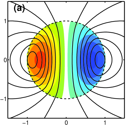
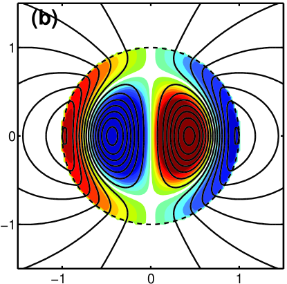
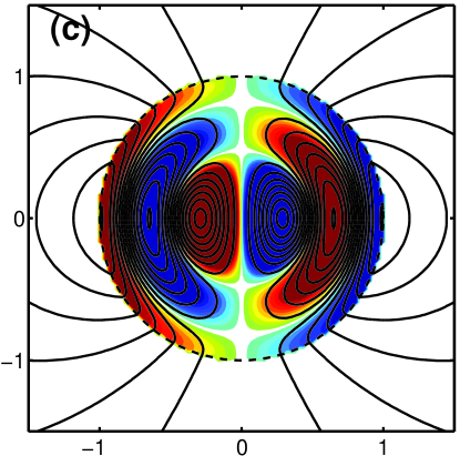
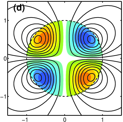
Figure 1: Meridional slices of illustrative magnetic field geometries for (a) the global minimum energy configuration, which corresponds to the first energy minimum of a dipole configuration, (b) & (c) the second and third energy minima of a dipole configuration, and (d) the lowest energy minimum of a quadrupole configuration. The poloidal and toroidal field structure are shown by the field lines and filled-color contours, respectively. In all plots the field line density is proportional to the poloidal flux and is normalized such that the average surface fields are equal. Similarly, the toroidal color scheme is uniform among all of the plots.

3.3 Energy and Helicity

For the values of $a_{l}$ and $\alpha$ found in the previous subsection, $S$ identically vanishes (substitute eq. 33 in eq. 32). As a consequence, in an energy minimum state, the magnetic helicity and energy are related by equation (11), exactly as for Woltjer states in uniform media. After integrating equation (60) for the magnetic energy, we find that

$$U=\alpha H=l(l+1)\alpha^{2}a_{l}^{2}/8\pi R^{2l-2}\,.$$ (35)

For a given fixed helicity $H$ and given $l$ and $\alpha$, this relation determines the value of $a_{l}$.

We have seen in the previous subsection that we have an infinite number of minimum energy solutions. This is because we are free to choose any value of the multipole index $l$, and for each $l$, we may choose any zero of $j_{l-1}$ (see eq. 34) to evaluate $\alpha$. Every one of these solutions is a local energy minimum with respect to variations of all quantities (including the fluid variables, see §1). Of these many local minima, one corresponds to the global energy minimum for the given magnetic helicity. Since $U=\alpha H$, the global minimum will have the smallest value of $\alpha$ among all the solutions, i.e., the smallest root of $j_{l-1}(z)$ for $l\geq 0$. By inspection it is clear that the global minimum energy solution has $l=1$ and $\alpha=\pi/R$, which corresponds to the first zero of $j_{0}(z)$. The magnetic field configuration of this solution corresponds to a dipole and is shown in Figure 1a. As mentioned, there are countless higher energy solutions, each of which corresponds to a local minimum. These involve higher multipoles and/or more complex radial structure. Some examples are shown in panels b–d of Figure 1, and are discussed in more detail in the following subsection.

As an aside, we note that these equilibrium configurations describe a class of solutions, defined by $\alpha R$ and $H$, as a function of $R$. Since $\alpha R$ and $H$ are fixed, $U\propto R^{-1}$. Therefore, if we were free to minimize $U$ with respect to $R$, we would find that $R\rightarrow\infty$ and $B\rightarrow 0$. This does not happen in practice because $R$ is also constrained by the self-gravity of the star. That is, we must minimize $U_{\rm tot}=U_{f}+U$ (see eq. 3) with respect to $R$, not $U$ alone. Generally, $U_{f}$ cannot be a monotonic function of $R$, otherwise no stable unmagnetized hydrostatic configuration would exist (which is a necessary a priori assumption). To illustrate this procedure, let us assume that $U\ll U_{f}$, and thus the correction to $R$ associated with the magnetic pressure is small (which will be shown below). Then, we may approximate $U_{f}$ and $U$ by

$$U_{f}\simeq U_{f,0}+\frac{1}{2}\frac{\partial^{2}U_{f}}{\partial R^{2}}\delta R^{2}\quad\text{and}\quad U\simeq U_{0}-U_{0}\frac{\delta R}{R_{0}}\,,$$ (36)

where $\delta R$ is the perturbation in the stellar radius as a result of the presence of the magnetic field. Thus, variations with respect to $\delta R$ give

$$\delta R\simeq\frac{U_{0}/R_{0}}{\partial^{2}U_{f}/\partial R^{2}}\sim\frac{U_{0}}{U_{f,0}}R_{0}\,.$$ (37)

Therefore, subdominant fields will correspond to a small perturbation to $R_{0}$ while equipartition fields will make corrections of order unity. However, it is clear that a stable configuration with finite $R$ and non-vanishing magnetic field does exist, and may be described by the analysis presented here.

3.4 Non-Equilibrium Configurations

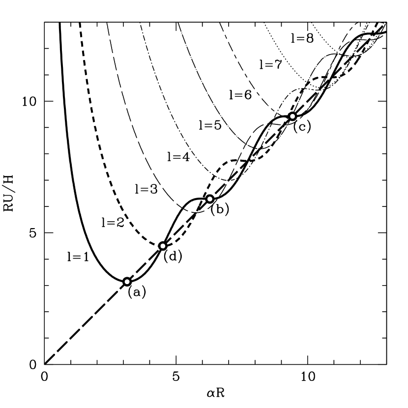
Figure 2: The energy per unit helicity as a function of the force-free constant, $\alpha$, both appropriately scaled by the stellar radius. The solid, short-dashed and long-dashed lines represent the first three multipoles, $l=1$, 2, 3, respectively. The dipole configuration with $\alpha R=\pi$, labelled (a), corresponds to the global minimum energy for a given helicity; the associated field geometry is shown in Figure 1a. There is a spectrum of higher energy local minima for each multipole, e.g., (b) and (c) for the dipole, which correspond to Figures 1b and 1c. The point labeled (d) is the minimum energy quadrupole configuration, and corresponds to Figure 1d. For reference, the diagonal line corresponds to $U=\alpha H$.

While we have found a globally optimized magnetic field geometry for a given magnetic helicity, thus far we have presumed that the star will naturally seek this minimum energy state via large scale motions and reconnection events. However, there is no guarantee that the star will not become trapped in higher energy, local equilibria, in which the necessary large scale rearrangements are inhibited. For this reason we consider a simple evolution, comprised of a single multipole and varying $\alpha$, which may occur, for instance, in some forms of current decay.

For values of $\alpha$ which are not zeros of $j_{l}(\alpha R)$ the action does not vanish. Nonetheless, it is straightforward to compute $U$ and use $S(\alpha R)$ to relate this to $H(\alpha)$:

$$U = \frac{l(l+1)}{8\pi R^{2l-1}}\alpha^{2}a_{l}^{2}\bigg{[}1-\frac{2l}{\alpha R}\frac{j_{l-1}(\alpha R)}{j_{l}(\alpha R)}+\frac{j_{l-1}^{2}(\alpha R)}{j_{l}^{2}(\alpha R)}\bigg{]},$$ (38)

$$H = \frac{U-S}{\alpha}$$ (39)

$$= \frac{l(l+1)}{8\pi R^{2l-1}}\alpha a_{l}^{2}\bigg{[}1-\frac{2l+1}{\alpha R}\frac{j_{l-1}(\alpha R)}{j_{l}(\alpha R)}+\frac{j_{l-1}^{2}(\alpha R)}{j_{l}^{2}(\alpha R)}\bigg{]}.$$

Since equilibria minimize the energy per unit helicity, we show in Figure 2 the quantity $RU/H$ as a function of $\alpha R$ for a number of multipoles. For each multiple there is a global minimum, with $U/H$ being smallest for the dipole. However, there are also a number of local minima corresponding to higher energy states. The explicit geometry for some of these are shown in Figure 1, and their implications are discussed in §3.8 and §4.

3.5 Solutions With no Toroidal Surface Stress

The solutions discussed so far are true minima of the total energy subject to a fixed helicity. Yet, they are not true equilibria of the system since they have unbalanced stresses at the stellar surface. This is a paradoxical situation — how can a minimum energy configuration not be in equilibrium? The explanation is that the motions that the surface stress will induce motions that cause an unwinding of the toroidal component of the magnetic field and thus a reduction in the magnetic helicity of the system. In effect, the unwinding of the field causes helicity to flow out of the star to infinity. Thus, while the solutions discussed so far are indeed true minimum energy states so long as helicity is conserved, they are not relevant for a fully fluid star because such a star does not preserve helicity.

One way to ensure helicity conservation is to make sure that there is no surface tangential stress, i.e., the toroidal magnetic field in the stellar interior vanishes as $r\to R$. By equation (26), this is easily arranged by having a field configuration with a single multipole $l$ and choosing $\alpha$ such that

$$j_{l}(\alpha R)=0,\qquad a_{l}\neq 0.$$ (40)

The situation is very similar to that of the minimum energy solutions discussed earlier, except that we now make use of a root of a different spherical Bessel function (cf. eqs. 34 and 40). These are simply the standard spheromak solutions, though we shall refer to them as zero-torque solutions to contrast them with the other solutions discussed throughout this paper.

As before, we have the option of choosing any value of $l$ and any zero of the corresponding Bessel function. Thus, we have an infinite number of possible solutions, of which that corresponding to $l=1$ and the first zero of $j_{1}(\alpha R)$ represents the overall lowest energy state. All these solutions have vanishing field in the exterior vacuum, as required by the matching condition (27), and they have no unbalanced tangential stress at the surface of the star. However, these configurations still require the presence of a rigid bounding crust. This is because they do have an unbalanced radial stress resulting from the discontinuity in the tangential field at the surface (it is non-zero inside and vanishes outside). Thus these configurations are also inappropriate for an entirely fluid star.

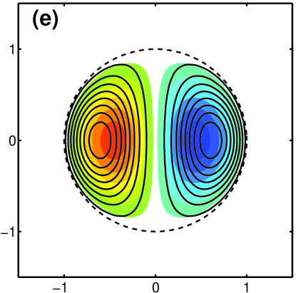
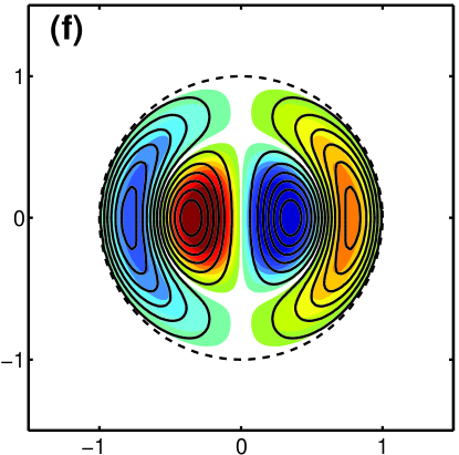
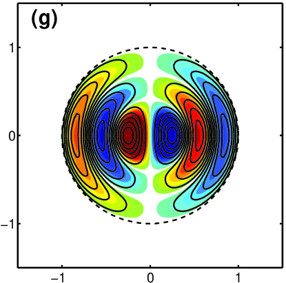
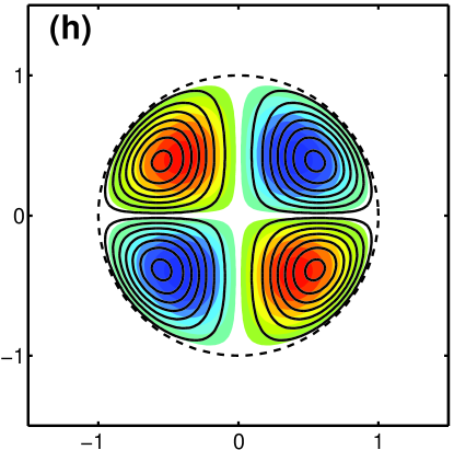
Figure 3: Meridional slices of illustrative magnetic field geometries with vanishing surface stresses for (e) the lowest energy such configuration, corresponding to the first dipole state, (f) & (g) the second and third dipole solutions, and (h) the lowest energy quadrupole configuration. The poloidal and toroidal field structure are shown by the field lines and filled-color contours, respectively. In all plots the field line density is proportional to the poloidal flux densities and the color scheme is proportional to the toroidal flux densities. Both are normalized such that all frames have identical total helicities. Note that there is no magnetic field outside the star.

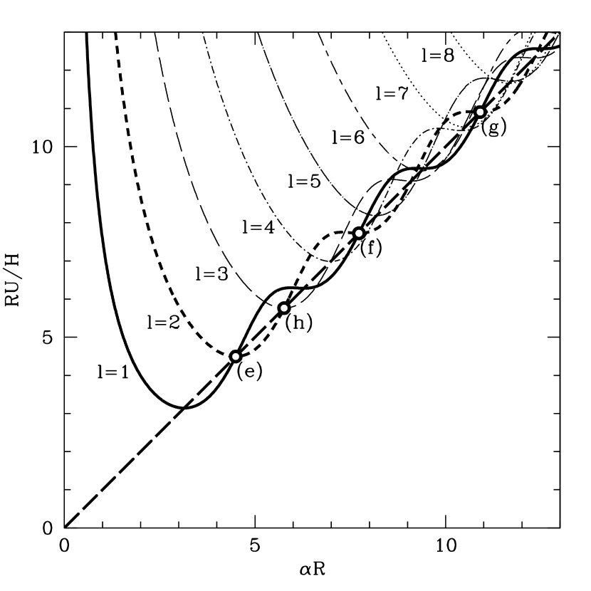
Figure 4: The same as Figure 2, except the zero-torque configurations shown in Figure 3 are labeled (e), (f), (g) (the first three dipole zero-torque states) and (h) (the first quadrupole zero-torque state). For reference, the diagonal line corresponds to $U=\alpha H$. Note that these solutions are not at minima in $U/H$, and thus are likely unstable.

Figure 3 shows meridional slices of the magnetic field corresponding to the first three zero-torque solutions with dipole geometry ($l=1$) and the first quadrupole solution ($l=2$). These solutions are very similar to the minimum energy solutions shown in Figure 1. The main difference is that the magnetic field is contained entirely inside the star and the field outside the star vanishes. Figure 4 is analogous to Figure 2, except that it highlights the solutions corresponding to the four panels in Figure 3. We note two interesting facts. First, the new solutions still satisfy $U=\alpha H$; hence, for a given $H$, the value of $\alpha$ directly gives the energy of the configuration. The lowest energy solution is the one with the smallest value of $\alpha$, i.e., solution (e) in Figures 3 and 4. Second, we see that the solutions do not live at minima of the energy with respect to $\alpha$ but rather at inflection points. This is because we determined the value of $\alpha$ from a boundary condition at $r=R$ rather than by minimizing the energy.

A system that reaches one of these zero-torque solutions will conserve helicity since there is no outward flow of helicity through the surface. However, it is not clear how long the system will survive in this state. Since there are neighboring solutions (with other values of $\alpha$) which have smaller values of the energy, the system is likely to evolve away from the zero-torque solution. Once it does this, the stress at the surface will no longer vanish and helicity will cease to be conserved. Whether or not this sequence of events can happen depends on the nature of the dynamical constraints that the fluid must satisfy, a topic that is beyond the scope of this paper.

3.6 Explicit Expressions for the Magnetic Field

In this subsection we provide for convenience explicit expressions for the magnetic field geometries of a few low-order multipole solutions, including those presented in Figures 1a-d and 3e-f.

Table 1: Approximate values of $\alpha R$ associated with various multipole solutions for the minimum energy (ME) and zero-torque (ZT) solutions, described by equations (41) and (43). Values associated with images shown are labeled by the corresponding figure number in the Notes column.

Model Type	$n$	$l$	$\alpha R$	Notes
ME	0	1	$\pi$	Global Energy Minimum, Fig. 1a
.	1	1	$2\pi$	Fig. 1b
.	2	1	$3\pi$	Fig. 1c
.	0	2	$4.4934$	Fig. 1d
.	1	2	$7.7253$	–
.	2	2	$10.904$	–
ZT	0	1	$4.4934$	Fig. 3e
.	1	1	$7.7253$	Fig. 3f
.	2	1	$10.904$	Fig. 3g
.	0	2	$5.7635$	Fig. 3h
.	1	2	$9.0950$	–
.	2	2	$12.323$	–

A natural normalization of the expressions obtained in sections 3.1 is in terms of the standard multipole field components of the surface magnetic field, $B_{l}$. In this case the exterior and interior field of a single multipole component is given by

$${\mn@boldsymbol{\rm B}}_{r\geq R}=B_{l}\left[\left(\frac{R}{r}\right)^{l+2}\mn@boldsymbol{\rm Y}_{l}-\frac{1}{l+1}\left(\frac{R}{r}\right)^{l+2}\mn@boldsymbol{\rm\Psi}_{l}\right]\,,$$ (41)

$${\mn@boldsymbol{\rm B}}_{r<R}=B_{l}\bigg{\{}\frac{Rj_{l}(\alpha r)}{rj_{l}(\alpha R)}\mn@boldsymbol{\rm Y}_{l}$$

$$\,\quad\qquad\qquad\qquad+\frac{\alpha Rrj_{l-1}(\alpha r)-lRj_{l}(\alpha r)}{l(l+1)rj_{l}(\alpha R)}\mn@boldsymbol{\rm\Psi}_{l}$$

$$\quad\qquad\qquad\qquad\qquad\qquad\qquad-\frac{\alpha R}{l(l+1)}\frac{j_{l}(\alpha r)}{j_{l}(\alpha R)}\mn@boldsymbol{\rm\Phi}_{l}\bigg{\}}\,.$$

The field may then be explicitly constructed given a value of $\alpha R$, and the explicit forms of the vector spherical harmonics and spherical Bessel functions given in Tables 2 and 3, respectively. The values of $\alpha R$ corresponding to the first few minimum energy (ME) multipole solutions are given in Table 1.

However, the normalization in equation (41) is divergent when the radial component of the surface field vanishes, and thus for the zero-torque solutions described in section 3.5 and shown in Figures 3 & 4. For these a better choice of normalization is in terms of the contribution of a given multipole to the total magnetic helicity, which simplifies to

$$H^{\rm zs}_{l}=\frac{B_{l}^{2}R^{4}}{8\pi l(l+1)}\alpha R\frac{j^{2}_{l-1}(\alpha R)}{j^{2}_{l}(\alpha R)}\,,$$ (42)

and also diverges for the zero-torque configurations [$j_{l}(\alpha R)=0$] when the strength of the radial component of the surface field ($B_{l}$) is held fixed. Explicitly, in terms of the contribution to the helicity, the solutions with vanishing surface stresses are given by

$${\mn@boldsymbol{\rm B}}_{r\geq R}=0\,,$$ (43)

$${\mn@boldsymbol{\rm B}}_{r<R}=\sum_{l}\sqrt{\frac{8\pi l(l+1)}{\alpha R^{5}}H^{\rm zs}_{l}}\bigg{\{}\frac{Rj_{l}(\alpha r)}{rj_{l-1}(\alpha R)}\mn@boldsymbol{\rm Y}_{l}$$

$$\,\quad\qquad\qquad\qquad+\frac{\alpha Rrj_{l-1}(\alpha r)-lRj_{l}(\alpha r)}{l(l+1)rj_{l-1}(\alpha R)}\mn@boldsymbol{\rm\Psi}_{l}$$

$$\quad\qquad\qquad\qquad\qquad\qquad\qquad-\frac{\alpha R}{l(l+1)}\frac{j_{l}(\alpha r)}{j_{l-1}(\alpha R)}\mn@boldsymbol{\rm\Phi}_{l}\bigg{\}}\,.$$

Note that since we used the vanishing surface stress limit for the helicity, the above expression is only valid for the configurations discussed in section 3.5. A more general expression can be normalized in terms of the helicity [eq. (39)], however this is correspondingly more complicated. The values of $\alpha R$ associated with the first few multipoles of the zero-torque (ZT) configurations are given in Table 1.

3.7 Star With a Rigid Crust

We now consider a star with a rigid crust that is able to support unbalanced magnetic surface stresses. The particular astrophysical system we have in mind is a magnetized neutron star. A rigid crust provides a firm anchor for any field lines that penetrate it. As a result, kinks in the magnetic field at the surface can survive indefinitely and there is no tendency for helicity to flow out to infinity. An additional effect of the crust is that any radial field component that is present at the stellar surface when the crust first forms will survive unchanged for a long time. This permanent surface field serves as a boundary condition at $r=R$.

We are then led to pose the following new problem: Given a fixed structure of the radial magnetic field at the stellar surface (i.e., values of the coefficients $a_{l}$) and a fixed total helicity of the system (the value of $H$), what are the equilibrium configurations of the magnetic field?

The magnetic field distribution exterior to the star is uniquely determined by the coefficients $a_{l}$. The solution in the interior of the star must be force-free and must therefore take the form (26), with the coefficients $d_{l}$ given by the matching condition (27). Therefore, the only free parameter in the solution is $\alpha$, and its value must be chosen such that the system has the required helicity $H$. The problem is thus quite similar to that posed in §3.5. The only difference is that, instead of having a vanishing field at the stellar surface, we now have a prescribed non-vanishing distribution of field strength at the surface.

It is useful to consider a specific numerical example. In the following, we have chosen the $a_{l}$ to scale as $l^{-5/6}/l(l+1)$, and thus $B_{l}^{2}\propto l^{-5/3}$, to crudely model the effect of a Kolmogorov turbulent cascade. Given a set of $a_{l}$ and a selected value of $\alpha$, equation (39) allows us to calculate the helicity of each multipole and equation (38) gives the corresponding energy. Moreover, since the vector spherical harmonics are mutually orthogonal, the total helicity and energy of the system are obtained by simply summing the contributions from the individual multipoles.

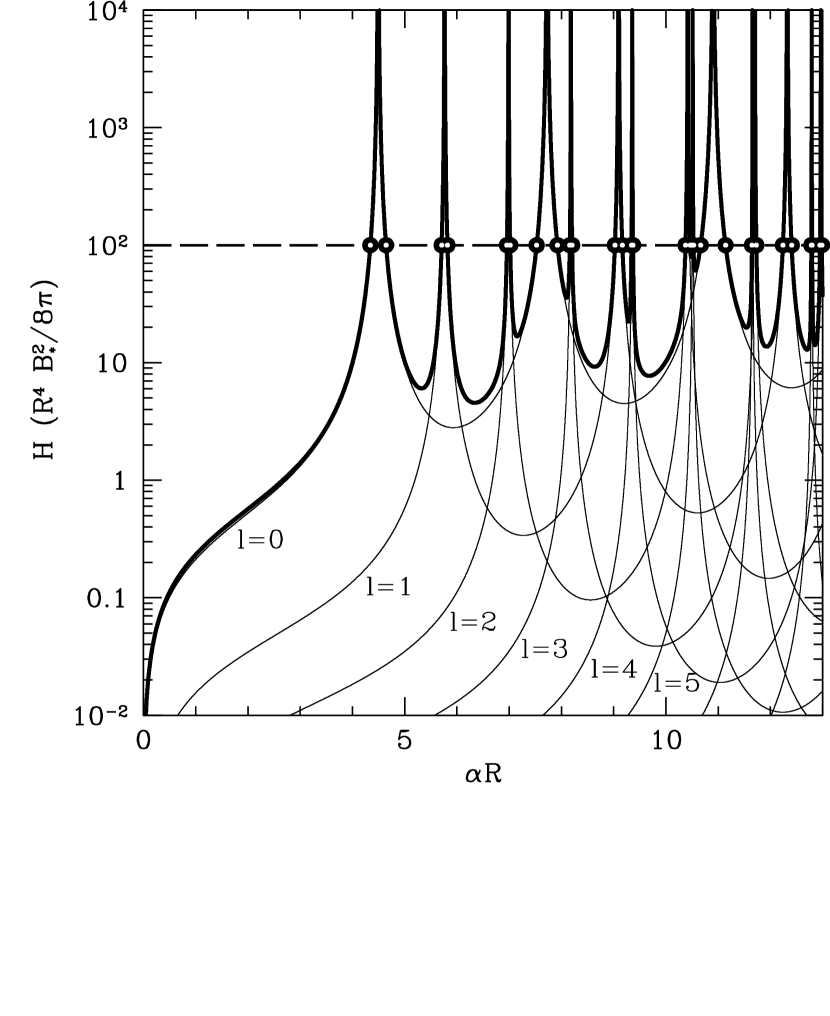
Figure 5: The helicity as a function of $\alpha R$ in units of the $B_{*}^{2}R^{4}/8\pi$ where $B_{*}$ is the normalization of the surface dipole field. The thin solid lines are the helicities of the individual modes, normalized by the Kolmogorov scaling described in the text. The thick solid line is the total helicity associated with the Kolmogorov spectrum. Also shown is a constant helicity of 100 by the long-dashed line, which crosses the helicity curve at a number of points. Note that the spikes in the helicity are due to the fact that we have fixed the magnitude of the exterior field, which implies that the interior field strength diverges at the zero-torque configurations.

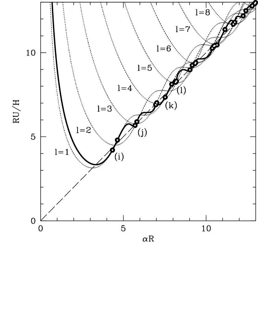
Figure 6: $U/H$ as a function of $\alpha R$ for the fixed Kolmogorov surface field spectrum described in the text. The points are states with $H=100$ as shown in Figure 5, and those that are explicitly shown in Figure 7 are labeled (i), (j), (k) and (l). Note that these are not necessarily energy minima, which is a direct result of fixing the multipolar structure at the stellar crust.

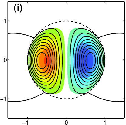
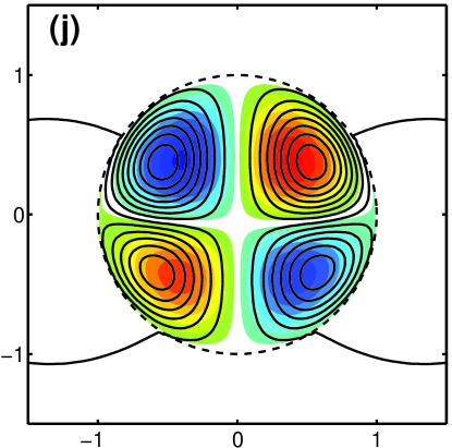
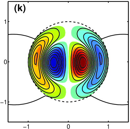
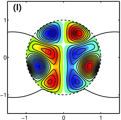
Figure 7: Meridional slices of a particular realization of the Kolmogorov spectrum described in the text for the states marked in Figure 6, each corresponding to a helicity of 100. In particular, (i), (j) and (k) show the first, third and seventh lowest energy states with a helicity of 100, while (l) shows the more complicated structures that can appear in higher energy states. The poloidal and toroidal field structure are shown by the field lines and filled-color contours, respectively. In all plots the field line density is proportional to the poloidal flux densities and the color scheme is proportional to the toroidal flux densities. Both are normalized such that all frames have identical total helicities. Note the similarities with Figure 3. Note also that all the panels have identical exterior field distributions.

Figure 5 shows the variation of total helicity (in appropriate units) as a function of $\alpha R$ for the numerical example described above. The many spikes in the curve correspond to the various zeros of $j_{l}(\alpha R)$; as equation (39) shows, the helicity diverges at these zeros. If the system has a certain conserved helicity $H$, which we have chosen to be 100 in the particular example shown in Figure 5, there will in general be multiple solutions for $\alpha$ which satisfy this constraint. Each of these is a valid solution to the problem. The solutions come in pairs, each bracketing a particular zero of a particular spherical Bessel function.

Figure 6 shows the energies of these solutions as given by equation (38). We see that the solutions are close to, and bracket, the zero-torque solutions shown in Figure 4. There is thus a close connection between the rigid-crust solutions and the zero-torque solutions. Finally, Figure 7 shows meridional slices of the magnetic field corresponding to the four solutions identified as (i), (j), (k) and (l) in Figure 6. The family resemblance of these solutions to those shown in Figure 3, and indeed also Figure 1, is obvious.

The strong similarity between the rigid-crust and zero-torque solutions is easy to understand. We have selected a somewhat large value of $H$ for the former, which means that the solutions must have a significantly larger field strength in the interior of the star compared to the surface, as is evident in Figure 7. In this situation, holding the surface field fixed at a small value (rigid-crust solutions) is nearly the same as setting the surface field to zero (zero-torque solutions).

3.8 Long Term Field Evolution

In the presence of a non-zero resistivity, the magnetic field will necessarily decay. Since, in practice, the resistive decay timescales are typically much longer than the Alfvén crossing time, we may approximate the state of the magnetic field as a series of non-equilibrium configurations, for which the general solution is given by equations (26) and (21). Furthermore, we will assume that the field begins in a local minimum energy configuration, where the large-scale structure prevents further fast reconnection.

As the field evolves due to resistive decay, the energy per unit helicity, $U/H$, will change as well. As a consequence, the value of $\alpha$ will evolve. This will generally result in the evolution of the magnetic field structure, provided the resistivity is not scale-invariant, i.e., small scale currents damp more rapidly than large scale currents. To see this consider Ohmic decay with a constant resistivity, $\rho$. In this case, the local field strength evolves according to

$$\dot{{\mn@boldsymbol{\rm B}}}=-{\mn@boldsymbol{\nabla}\times}{\mn@boldsymbol{\rm E}}=-\rho{\mn@boldsymbol{\nabla}\times}{\mn@boldsymbol{\rm J}}=-\frac{\rho}{4\pi}{\mn@boldsymbol{\nabla}\times}{\mn@boldsymbol{\nabla}\times}{\mn@boldsymbol{\rm B}}=-\frac{\alpha^{2}\rho}{4\pi}{\mn@boldsymbol{\rm B}}\,.$$ (44)

Upon inserting equation (26) into this, we find

$$\dot{a}_{l}=-\frac{\alpha^{2}\rho}{4\pi}a_{l}\qquad\text{and}\qquad\dot{\alpha}=0\,,$$ (45)

i.e., the magnetic field strength (proportional to $a_{l}$) decreases, but the structure (described by $\alpha$) remains unchanged.

However, if the poloidal currents decay more rapidly than the toroidal currents, e.g., due to enhanced dissipation of the surface currents or because dissipation is non-linear, $\alpha$ will be time dependent. This is clear from equation (26), in which $B^{\phi}/B^{r}\propto\alpha$. Thus if poloidal currents (and hence toroidal magnetic fields) decay more rapidly than toroidal currents (and hence poloidal magnetic fields), $\dot{\alpha}<0$ and the magnetic field configuration will move to the left in Figures 2, 4 and 6. When the system evolves out of a local equilibrium state a substantial amount of magnetic energy is necessarily liberated. The natural timescale over which this energy is released is the Alfén crossing time, though we do not address the details of the instability here.

Finally, note that in the presence of a conducting magnetosphere with an infinitely conductive surface a fluid star would appear as a uniform medium. This is despite the fact that the magnetosphere has a much lower density than the stellar interior, and thus is always described by force-free dynamics. This disparity results in very different dynamical times for the two regions. Nevertheless, since currents can freely flow between the stellar interior and the magnetosphere, the minimum energy equilibrium configuration will be described by that for a uniform medium, which has no stable equilibrium magnetic field configuration for any value of magnetic helicity. That is, in this case $\alpha=U/H$ can take any value, including zero. Thus such a field is unconditional unstable. Whether or not this occurs in the context of a stellar field depends upon the conductivity of the surface, the exterior, and the ability of the crust to fix the magnetic field.

4 Discussion and Application to Neutron Stars

4.1 General Discussion

Although we have described three different kinds of solutions — minimum-energy solutions (§3.2), zero-torque solutions (§3.5) and rigid-crust solutions (§3.7) — all have certain features in common.

For each class of solutions, the lowest energy state (“ground state”), subject to a fixed total helicity, is dominated by a dipolar field configuration. Nevertheless, within the context of a magnetic relaxation model, the presence of higher order multipoles is not unexpected. After the cessation of a dynamo in the early history of a star, the resulting magnetic field will be chaotic and highly tangled over a wide range of scales. The field will also be violently unstable, decaying rapidly towards a local minimum energy configuration. However, as described in §3.8, this will only proceed as long as the rearrangement is driven by small scale reconnection. Large scale rearrangements, such as converting low-order multipoles into dipoles, will occur over the much longer resistive timescale. As a consequence, we generally expect the resulting field to be dominated by a dipole component with significant quadrupolar and octupolar components. This is consistent with the outcome of numerical simulations (Braithwaite & Spruit, 2004).

A novel feature of our work is the identification of higher-energy quasi-equilibrium states. At late times, small-scale current decay will drive the system to evolve towards smaller $\alpha$, necessarily resulting in periods of violent instability when the system hops from one quasi-equilibrium state to the next. These will result in large scale reorganizations of the internal and external stellar magnetic fields over Alfvénic timescales. As a consequence, these events could power active periods in which a substantial fraction of the stellar magnetic energy is released.

Since the quasi-equilibria of the dipole state are located at zeros of low-order spherical Bessel functions, the magnetic energy release in these events should be roughly quantized (though the system may jump over many local equilibria in a single event), releasing an energy of order $k\pi H/R$ for some integer $k$. The observed energy release will depend strongly upon the emission mechanism and will likely not appear strictly quantized. Nevertheless, this model implies a lower limit upon the energy that can be released during an outburst, simply given by the energy of the global minimum energy configuration.

The minimum-energy solutions described in §3.2 and Figures 1, 2, have a toroidal kink in the magnetic field at the stellar surface, in apparent contrast to numerical simulations (cf. Yoshida et al., 2006; Braithwaite & Spruit, 2004). The toroidal field discontinuity will lead to a non-radial surface stress, which cannot be balanced by a fluid star. Thus, these solutions are probably not of practical interest.

The zero-torque solutions described in §3.5 and Figures 3, 4, are more promising. They are perfectly force-free solutions with no unbalanced stresses. However, they have some deficiencies. First, they have no magnetic field outside the star. Therefore, they are not very useful for understanding the observed exterior field of systems such as magnetic A stars and white dwarfs. Second, these solutions are not minimum energy states of the force-free problem. Therefore, a star in one of these states could, in principle, lower its energy by evolving to a nearby configuration with a lower value of $\alpha$. The neighboring lower-energy state will not be stress-free at the surface and the system may thus develop a dynamical instability. Whether or not this will happen in a real system depends on dynamical constraints which we cannot address. Modulo this caveat, the zero-torque solutions are of possible interest for understanding the numerical work of Braithwaite & Spruit (2004).

All the solutions we have described in this paper have a constant $\alpha$ in the stellar interior. This is a natural consequence of the variational approach we have taken, which is based on the principle of conservation of total helicity (Taylor, 1974), but it is not necessarily appropriate for a magnetized star. We could, in principle, consider solutions in which a part of the stellar interior has a non-zero value of $\alpha$ and contains all the toroidal field and helicity, while the rest of the star has $\alpha=0$ and purely poloidal structure. Such solutions are more difficut to construct, but may be able to produce stable configurations with no stress at the surface. An even more extreme scenario is to consider a separately conserved microscopic helicity for each magnetic flux tube (see Appendix A). These topics are beyond the scope of this paper.

4.2 Neutron Stars

During their birth, neutron stars are expected to have convectively driven dynamos and to develop extremely strong magnetic fields, as high as $10^{15-16}\,{\rm G}$. However, shortly afterward, and prior to the development of a solid crust, the dynamo action ceases and the nascent neutron star magnetic field evolves for roughly $100\,{\rm s}$. During this time magnetic relaxation will play a central role in determining the strength and structure of the magnetic field. Once the crust forms, the magnetic field at the surface of the star is frozen in and the magnetic helicity of the system is fixed. Further evolution of the system is likely governed by total helicity conservation, coupled with the requirement that the radial field at the stellar surface is fixed. These are precisely the conditions we have assumed in deriving the rigid-crust solutions discussed in §3.7 and Figures 5–7.

Generally, we expect a dominant dipole field structure, with non-negligible quadrupole and octupole components. Since the magnetic helicity is a scalar quantity, we naturally expect a non-aligned magnetic field with respect to the rotation axis. For a highly tangled initial field (with considerable power on small-scales), we would expect the orientation of the birth fields of neutron stars to be uniformly distributed relative to the spin axis. This provides a natural way in which to produce the off-axis fields required for understanding radio and X-ray pulsars.

For a system with non-zero total helicity, since any magnetic field at the stellar surface will generally have an associated toroidal stress, we speculate that the fluid neutron star before the formation of the crust will evolve through states in which the surface field is generally weak relative to the field in the interior. This condition will be frozen in once the crust forms. Thus, the frozen-in helicity will be large compared to the characteristic helicity we might expect based on the magnitude of $B_{s}$, the surface field strength: $H\gg(B_{s}^{2}/8\pi)R^{4}$. Similarly, the magnetic energy will also be large: $U\gg(B_{s}^{2}/8\pi)R^{3}$. These are the conditions we assumed for the examples shown in Figures 5–7.

Once the crust forms, the system will settle down into the nearest available solution, which would presumably correspond to a relatively large value of $\alpha$. Subsequently, we imagine that the magnetic field will evolve via sudden jumps from one solution to the next, with a steady reduction in the magnitude of $\alpha$. Each jump will cause a decrease in the total magnetic energy and a corresponding increase in the thermal energy of the star. The leaking of this thermal energy out of the star will power thermal X-ray emission from the surface. This may explain the quasi-steady X-ray emission seen in anomalous X-ray pulsars (AXPs) and other magnetars.

It is interesting to note that the source of this thermal energy is by its very nature non-steady. Bursts of energy are released each time the interior magnetic field switches from one state to the next. Although the flux escaping from the surface will be smoothed on the thermal diffusion time, some variability is expected and is indeed seen in magnetars.

Furthermore, as we see from Figures 5 and 6, neighboring solutions are bunched more closely together for larger values of $\alpha$ and are farther apart at lower $\alpha$. Since the magnetic energy is to a good approximation proportional to $\alpha$ (see Fig. 6), we expect frequent small bursts of energy early in the life of the neutron star, when $\alpha$ is large, and rarer but more powerful bursts later on. Thus, there should be less variability in younger systems and larger fluctuations in older systems, with the most dramatic variations occurring in the oldest magnetars.

The above discussion was concerned with magnetic field evolution in the interior of the star with a fixed surface field. However, since the star has a much sronger field in its interior compared to the surface, we expect the crust occasionally to crack under the pressure and to release some of the enclosed energy and helicity in a sudden cataclysmic event. These events dump a lot of energy near the surface of the star and provide a natural mechanism for powering bursts associated with soft-gamma repeaters (SGRs). With typical energies ranging from $10^{36-46}\,{\rm erg}$, SGR bursts require interior magnetic fields on the order of $10^{9-14}\,{\rm G}$, which are considerably less than the equipartition values that are possible as a result of magnetar formation (Thompson & Duncan, 1993; Spruit, 2002). For magnetars, the Alfvén crossing time is on the order of a second, corresponding to maximum luminosities on the order of $10^{46}~{}{\rm erg\,s^{-1}}$. If this energy is thermalized in the neutron star crust over the Alfvén timescale, it would result in surface temperatures on the order of roughly an ${\rm M}{\rm eV}$, similar to what is seen in SGR flares. However, the precise details of the emission will depend upon the details of the emission mechanism (see, e.g., Thompson et al., 2002; Lyutikov, 2006).

As in the case of internal field rearrangements, we expect the most violent events to occur somewhat late in the life of a magnetar, when the interior field is dominated by lower multipoles. Thus, the strongest outbursts should be seen in relatively old systems. All of these arguments suggest that SGRs as a class might be older than AXPs.

In this picture magnetars are born with magnetic fields in configurations that are local equilibria at strengths orders of magnitude larger than the global minimum. If we assume that the minimum energy of observed SGR bursts is indicative of the energy scale of the power source, this implies that the field strength in this minimum energy state is roughly $10^{9}\,{\rm G}$. Hence, the SGR bursts would be the result of the decay of the internal magnetic field, resulting finally in a stable field strength commensurate with millisecond pulsars. Note that this is a different mechanism than that described in Braithwaite & Spruit (2006).

Appendix A Relationship to Other Variational Principles

We present a particular variational principle, with the somewhat surprising result (though similar to that found in Woltjer, 1962) that the minimum energy states of the magnetic field correspond to a completely force-free state in the stellar interior with uniform force-free constant, $\alpha$. This is surprising since equilibrium configurations that balance magnetic stresses against fluid pressure are conspicuously absent from our approach. Thus it is worthwhile to discuss the particular conditions that our solution is valid under and why this differs from those derived under the assumption of ideal MHD.

Our variational principle differs explicitly from that described in Field 1986 (an interesting paper brought to our attention by the anonymous referee). The latter reproduces the standard MHD relation, balancing pressure against magnetic stresses, leading the author to argue that the result of Woltjer (1962) is only valid if the pressure is uniform throughout the fluid. This variational principle is derived in a fashion nearly identical to that presented in section 2, minimizing the total energy (fluid and magnetic) subject to a condition upon the helicity. However there are two important distinctions.

The first concerns the terms in the fluid component of the energy. Field (1986) ignores the contributions due to self-gravity. As a consequence pressure gradients can only be balanced by the Lorentz force. This generally will result in an unconditionally unstable system for isolated magnetized fluids. In contrast, a self-gravitating magnetized fluid can balance pressure gradients against the gravitational acceleration, and thus the Lorentz force may in principle vanish. Therefore, when we include self-gravity, the existence of pressure gradients is not synonymous with the magnetic field violating force-free (see, e.g.,  Chandrasekhar & Prendergast, 1956)

The second concerns the way in which helicity conservation is imposed. In ideal MHD it is possible to define a conserved microscopic magnetic helicity associated with each magnetic flux tube. Therefore, we may in principle seek to impose conservation of not only the macroscopic, volume integrated helicity, but the helicity associated with each field loop separately, i.e. take $\alpha$ not to be a constant, but to be a function of position. This is precisely the constraint imposed in Field (1986).

However, it is far from clear that in the presence of large-scale dissipation that this is the correct prescription. Indeed, the conjecture by Taylor (1974), apparently supported by spheromak experiments, is that this be replaced with a volume-integrated constraint, of the form we have employed. The reason given by Taylor (1974) for this is that the microscopic helicity associated with each flux tube is not conserved during reconnection events. Indeed, during reconnection, flux tubes with different helicities may be combined, changing the total helicity of the new loop (the precise manner in which this occurs is not clearly defined since the evolutionary equation for the flux-tube helicity depends upon the way in which helicity proceeds). However, reconnection will not change the macroscopic topology of the magnetic field, and therefore the total helicity will be preserved.

An alternative way to justify this is to note that if the magnetic field rapidly reconnects, it is impossible to define unique magnetic field loops. That is, after sufficient time each magnetic field loop will have been connected with every other remaining loop at some point in the reconnection history. As a consequence, the force-free constant (i.e., $\alpha$) associated with each loop will necessarily be the same, since this is constant along magnetic field lines. This will remain to be the case unless the helicity along some subset of field lines can preferentially decay (which is the case in the absence of a rigid crust).

These differences explain the absence of solutions which balance magnetic stresses and pressure gradients in our formalism. Such solutions require additional constraints, such as flux freezing in ideal MHD, which inhibit the movement of magnetic field lines through the fluid. By considering the high-dissipation/rapid-reconnection limit via our volume constraint upon the total magnetic helicity we have necessarily ignored such constraints. That is, in the absence of such additional constraints there are no stable configurations which balance magnetic stresses against pressure gradients, since the fluid and magnetic field will move through each other until such gradients are erased. (This is identical to equilibrium configuration of a two-component ideal gas, in which both species separately satisfy the equilibrium condition.) In the rapidly reconnecting limit, the magnetic field can globally reconfigure on short timescales, and thus we are justified in treating the magnetic field and fluid as non-interacting in this fashion. Finally, because we are restricting our attention to gravitationally bound objects, non-vanishing pressure gradients may be balanced against self-gravity, and therefore do not require violations of the force-free condition to maintain equilibrium.

Appendix B Force-Free Fields in Uniform Media

When the medium is uniformly infinitely conductive (i.e., the currents required by the resulting magnetic field satisfy any physical restrictions) the quantity to be minimized is

$$S=\int_{V}\frac{1}{8\pi}\left({\mn@boldsymbol{\rm B}}\cdot{\mn@boldsymbol{\rm B}}-\alpha{\mn@boldsymbol{\rm A}}\cdot{\mn@boldsymbol{\rm B}}\right){{\rm d}^{3}\!x}\,,$$ (46)

where the constraint upon the total helicity is included via the Lagrange multiplier $\alpha$. As originally discussed in Woltjer (1958) (and thus frequently referred to as the Woltjer state) variations with respect to ${\mn@boldsymbol{\rm A}}$ produce the familiar force-free equation ${\mn@boldsymbol{\nabla}\times}{\mn@boldsymbol{\rm B}}=\alpha{\mn@boldsymbol{\rm B}}$ for the magnetic field. That this produces a force-free field is not unexpected; non-force-free perturbations to a force-free solution necessarily require work to be done upon, and thus energy added to, the magnetic field. For the purpose of comparison with what follows we will derive this equation below.

First note that

$$\delta({\mn@boldsymbol{\rm B}}\cdot{\mn@boldsymbol{\rm B}}) =2\delta{\mn@boldsymbol{\rm A}}\cdot({\mn@boldsymbol{\nabla}\times}{\mn@boldsymbol{\rm B}})-2{\mn@boldsymbol{\nabla}\cdot}({\mn@boldsymbol{\rm B}}\times\delta{\mn@boldsymbol{\rm A}})\,,$$ (47)

$$\delta({\mn@boldsymbol{\rm A}}\cdot{\mn@boldsymbol{\rm B}}) =2\delta{\mn@boldsymbol{\rm A}}\cdot({\mn@boldsymbol{\nabla}\times}{\mn@boldsymbol{\rm A}})-{\mn@boldsymbol{\nabla}\cdot}({\mn@boldsymbol{\rm A}}\times\delta{\mn@boldsymbol{\rm A}})\,.$$

Therefore,

$$8\pi\delta S= \int_{V}\delta{\mn@boldsymbol{\rm A}}\cdot\left({\mn@boldsymbol{\nabla}\times}{\mn@boldsymbol{\rm B}}-\alpha{\mn@boldsymbol{\nabla}\times}{\mn@boldsymbol{\rm A}}\right){{\rm d}^{3}\!x}$$ (48)

$$-\oint_{\partial V}\left({\mn@boldsymbol{\rm B}}\times\delta{\mn@boldsymbol{\rm A}}-\frac{\alpha}{2}{\mn@boldsymbol{\rm A}}\times\delta{\mn@boldsymbol{\rm A}}\right)\cdot{{\rm d}\mn@boldsymbol{S}}$$

$$= \int_{V}\delta{\mn@boldsymbol{\rm A}}\cdot\left({\mn@boldsymbol{\nabla}\times}{\mn@boldsymbol{\rm B}}-\alpha{\mn@boldsymbol{\rm B}}\right){{\rm d}^{3}\!x}$$

$$-\oint_{\partial V}\delta{\mn@boldsymbol{\rm A}}\cdot\left[{\mn@boldsymbol{\hat{\rm n}}}\times\left({\mn@boldsymbol{\rm B}}-\frac{\alpha}{2}{\mn@boldsymbol{\rm A}}\right)\right]{{\rm d}^{2}\!x}\,,$$

where ${\mn@boldsymbol{\hat{\rm n}}}$ is the normal to the surface defined by $\partial V$ and ${{\rm d}^{2}\!x}$ is defined by ${{\rm d}\mn@boldsymbol{S}}\equiv{\mn@boldsymbol{\hat{\rm n}}}\,{{\rm d}^{2}\!x}$. Note that the surface integral is generally gauge dependent. This can be cured if $\delta{\mn@boldsymbol{\rm A}}$ is constrained to vanish at $\partial V$. Since in what follows we will set $\partial V$ to infinity and the energy in the field will necessarily be finite, a gauge will necessarily exist in which ${\mn@boldsymbol{\rm A}}$ vanishes on $\partial V$, and thus this constraint upon $\partial V$ is justified. Therefore, the desired magnetic field must satisfy

$${\mn@boldsymbol{\nabla}\times}{\mn@boldsymbol{\rm B}}=\alpha{\mn@boldsymbol{\rm B}}\,.$$ (49)

Equation (49) implies that

$${\mn@boldsymbol{\nabla}\times}({\mn@boldsymbol{\rm B}}-\alpha{\mn@boldsymbol{\rm A}})=0\quad\rightarrow\quad\alpha{\mn@boldsymbol{\rm A}}={\mn@boldsymbol{\rm B}}+\alpha{\mn@boldsymbol{\nabla}}\Lambda\,,$$ (50)

and thus a natural gauge choice for non-zero $\alpha$ is the “force-free” gauge defined by $\Lambda=0$. Note that this is also a Lorentz gauge since ${\mn@boldsymbol{\nabla}\cdot}{\mn@boldsymbol{\rm B}}=0$.

Within the force-free gauge it is straightforward to show that the helicity and minimum possible magnetic energy are proportional. That is,

$$H=\int_{V}\frac{1}{8\pi}{\mn@boldsymbol{\rm A}}\cdot{\mn@boldsymbol{\rm B}}\,{{\rm d}^{3}\!x}=\int_{V}\frac{1}{8\pi}\alpha^{-1}{\mn@boldsymbol{\rm B}}\cdot{\mn@boldsymbol{\rm B}}\,{{\rm d}^{3}\!x}=\alpha^{-1}U\,,$$ (51)

and thus small $\alpha$ correspond to small $U$ for the same $H$.

Appendix C Boundary Conditions

On the boundaries between type-I and type-II regions, the fields must satisfy the usual boundary conditions:

$${\mn@boldsymbol{\hat{\rm n}}}\cdot\left({\mn@boldsymbol{\rm B}}_{\rm I}-{\mn@boldsymbol{\rm B}}_{\rm II}\right)=0\quad\text{and}\quad{\mn@boldsymbol{\hat{\rm n}}}\times\left({\mn@boldsymbol{\rm B}}_{\rm I}-{\mn@boldsymbol{\rm B}}_{\rm II}\right)=\frac{4\pi}{c}\mn@boldsymbol{K}\,,$$ (52)

where ${\mn@boldsymbol{\hat{\rm n}}}$ is the surface normal (directed from I to II) and $\mn@boldsymbol{K}$ is the induced surface current density. The proper surface current can be found by explicitly constructing solutions and minimizing the magnetic energy. Note that this ignores any energy associated with the surface currents themselves.

However, this should also emerge naturally from the equations (6) and (7). The first is obtained from ${\mn@boldsymbol{\nabla}\cdot}{\mn@boldsymbol{\rm B}}=0$, which is true by definition and may be verified by taking the divergence of equation (6). The second is obtained via integrating equation (6) around an infinitesimal loop crossing the surface. Define a local Cartesian coordinate system at the position of interest at the I-II boundary in which ${\mn@boldsymbol{\hat{\rm z}}}\parallel{\mn@boldsymbol{\hat{\rm n}}}$ at the boundary, at which $z=0$. Then, upon integrating around a rectangular loop in the $x$-$z$ plane of length $\ell$ in the ${\mn@boldsymbol{\hat{\rm x}}}$-direction and vanishing length in the ${\mn@boldsymbol{\hat{\rm z}}}$-direction, we find

$$\left({\mn@boldsymbol{\rm B}}_{\rm I}-{\mn@boldsymbol{\rm B}}_{\rm II}\right)\cdot\ell{\mn@boldsymbol{\hat{\rm x}}} =\oint_{C}{\mn@boldsymbol{\rm B}}\cdot{\mn@boldsymbol{{\rm d}\ell}}=\int_{A}\left({\mn@boldsymbol{\nabla}\times}{\mn@boldsymbol{\rm B}}\right)\cdot{{\rm d}\mn@boldsymbol{S}}$$ (53)

$$=\int_{A}\left(\alpha{\mn@boldsymbol{\rm B}}-{\mn@boldsymbol{\nabla}\times}{\mn@boldsymbol{\nabla}\times}f{\mn@boldsymbol{\lambda}}\right)\cdot{{\rm d}\mn@boldsymbol{S}}$$

$$=\oint_{C}\left(\alpha{\mn@boldsymbol{\rm A}}+{\mn@boldsymbol{\lambda}}\times{\mn@boldsymbol{\nabla}}f-f{\mn@boldsymbol{\nabla}\times}{\mn@boldsymbol{\lambda}}\right)\cdot{\mn@boldsymbol{{\rm d}\ell}}$$

$$=\oint_{C}\left[(1-f)\alpha{\mn@boldsymbol{\rm A}}-f\alpha{\mn@boldsymbol{\nabla}}\Lambda+{\mn@boldsymbol{\lambda}}\times{\mn@boldsymbol{\nabla}}f\right]\cdot{\mn@boldsymbol{{\rm d}\ell}}\,.$$

The third term in the integrand can be integrating after noting ${\mn@boldsymbol{\nabla}}f={\mn@boldsymbol{\hat{\rm z}}}\delta(z)$ by definition, and thus

$$\oint_{C}\delta(z){\mn@boldsymbol{\lambda}}\times{\mn@boldsymbol{\hat{\rm z}}}\cdot{\mn@boldsymbol{{\rm d}\ell}}=\left(\lambda\times{\mn@boldsymbol{\hat{\rm z}}}\right)\cdot{\mn@boldsymbol{\hat{\rm z}}}=0\,.$$ (54)

Despite the explicit presence of the vector potential, the first two terms in the integrand are indeed gauge independent. Explicitly, note that since under the gauge transformation ${\mn@boldsymbol{\rm A}}\rightarrow{\mn@boldsymbol{\rm A}}+{\mn@boldsymbol{\nabla}}\Lambda^{\prime}$ also implies that $\Lambda\rightarrow\Lambda-\Lambda^{\prime}$, and hence

$$(1-f)\alpha{\mn@boldsymbol{\rm A}}-f\alpha{\mn@boldsymbol{\nabla}}\Lambda\rightarrow(1-f)\alpha{\mn@boldsymbol{\rm A}}-f\alpha{\mn@boldsymbol{\nabla}}\Lambda+{\mn@boldsymbol{\nabla}}\Lambda^{\prime}\,.$$ (55)

Finally, noting that $\int_{C}{\mn@boldsymbol{\nabla}}\Lambda^{\prime}\cdot{\mn@boldsymbol{{\rm d}\ell}}=0$ completes the proof.

Therefore,

$$\left({\mn@boldsymbol{\rm B}}_{\rm I}-{\mn@boldsymbol{\rm B}}_{\rm II}\right)\cdot\ell{\mn@boldsymbol{\hat{\rm x}}}=\alpha{\mn@boldsymbol{\rm A}}_{\rm I}\cdot\ell{\mn@boldsymbol{\hat{\rm x}}}+\alpha\ell{\mn@boldsymbol{\hat{\rm x}}}\cdot{\mn@boldsymbol{\nabla}}\Lambda$$ (56)

With an analogous expression for a loop in the $y$-$z$ plane, the surface current is given by

$$\frac{4\pi}{c}\mn@boldsymbol{K}=\alpha{\mn@boldsymbol{\hat{\rm n}}}\times\left({\mn@boldsymbol{\rm A}}_{\rm I}+{\mn@boldsymbol{\nabla}}\Lambda\right)\,.$$ (57)

If we choose the force-free gauge within regions of type-I, continuity of the vector potential gives

$$\frac{4\pi}{c}\mn@boldsymbol{K}={\mn@boldsymbol{\hat{\rm n}}}\times\left({\mn@boldsymbol{\rm B}}_{\rm I}+\alpha{\mn@boldsymbol{\nabla}}\Lambda\right)\,,$$ (58)

or,

$${\mn@boldsymbol{\hat{\rm n}}}\times\left({\mn@boldsymbol{\rm B}}_{\rm II}-\alpha{\mn@boldsymbol{\nabla}}\Lambda\right)=0\,,$$ (59)

on the boundary. That is, as expected ${\mn@boldsymbol{\rm B}}_{\rm II}$ is a potential field, though otherwise the surface currents are unconstrained.

Appendix D The Action in Non-Uniform Media

In non-uniform medium, it is possible to explicitly reduce the computation of the action to integrals over the boundaries between conducting (type-I) and insulating (type-II) regions. To do this, first note that the magnetic energy is given by

$$U =\int_{\rm I}\frac{1}{8\pi}{\mn@boldsymbol{\rm B}}\cdot{\mn@boldsymbol{\rm B}}\,{{\rm d}^{3}\!x}+\int_{\rm II}\frac{1}{8\pi}{\mn@boldsymbol{\rm B}}\cdot{\mn@boldsymbol{\nabla}}\varphi\,{{\rm d}^{3}\!x}$$ (60)

$$=\int_{\rm I}\frac{1}{8\pi}{\mn@boldsymbol{\rm B}}\cdot{\mn@boldsymbol{\rm B}}\,{{\rm d}^{3}\!x}-\oint_{\partial({\rm I-II})}\frac{1}{8\pi}\varphi{\mn@boldsymbol{\rm B}}\cdot{{\rm d}\mn@boldsymbol{S}}\,,$$

where ${\mn@boldsymbol{\nabla}\cdot}{\mn@boldsymbol{\rm B}}=0$ was used. Note that because the ${\mn@boldsymbol{\hat{\rm n}}}\cdot{\mn@boldsymbol{\rm B}}$ is continuous across the boundary, this may be evaluated using only type-I quantities.

If $\Lambda_{\rm L}$ is defined by ${\mn@boldsymbol{\rm A}}={\mn@boldsymbol{\rm A}}_{\rm L}+{\mn@boldsymbol{\nabla}}\Lambda_{\rm L}$ where ${\mn@boldsymbol{\rm A}}_{\rm L}$ is in the Lorentz gauge (i.e., ${\mn@boldsymbol{\nabla}\cdot}{\mn@boldsymbol{\rm A}}_{\rm L}=0$), the magnetic helicity is given by

$$H =\int_{\rm I}\frac{1}{8\pi}{\mn@boldsymbol{\rm A}}\cdot{\mn@boldsymbol{\rm B}}\,{{\rm d}^{3}\!x}+\int_{\rm II}\frac{1}{8\pi}{\mn@boldsymbol{\rm A}}\cdot{\mn@boldsymbol{\nabla}}\varphi\,{{\rm d}^{3}\!x}$$ (61)

$$=\alpha^{-1}\int_{\rm I}\frac{1}{8\pi}{\mn@boldsymbol{\rm B}}\cdot{\mn@boldsymbol{\rm B}}\,{{\rm d}^{3}\!x}-\oint_{\partial({\rm I-II})}\frac{1}{8\pi}\varphi{\mn@boldsymbol{\rm A}}\cdot{{\rm d}\mn@boldsymbol{S}}$$

$$\qquad-\int_{\rm II}\frac{1}{8\pi}\varphi{\mn@boldsymbol{\nabla}\cdot}{\mn@boldsymbol{\rm A}}\,{{\rm d}^{3}\!x}$$

$$=\alpha^{-1}\int_{\rm I}\frac{1}{8\pi}{\mn@boldsymbol{\rm B}}\cdot{\mn@boldsymbol{\rm B}}\,{{\rm d}^{3}\!x}-\alpha^{-1}\oint_{\partial({\rm I-II})}\frac{1}{8\pi}\varphi{\mn@boldsymbol{\rm B}}\cdot{{\rm d}\mn@boldsymbol{S}}$$

$$\qquad-\int_{\rm II}\frac{1}{8\pi}\varphi\nabla^{2}\Lambda_{\rm L}\,{{\rm d}^{3}\!x}$$

$$=\alpha^{-1}U+\oint_{\partial({\rm I-II})}\frac{1}{8\pi}\varphi{\mn@boldsymbol{\nabla}}\Lambda_{\rm L}\cdot{{\rm d}\mn@boldsymbol{S}}+\int_{\rm II}\frac{1}{8\pi}{\mn@boldsymbol{\rm B}}\cdot{\mn@boldsymbol{\nabla}}\Lambda_{\rm L}$$

$$=\alpha^{-1}U-\oint_{\partial({\rm I-II})}\frac{1}{8\pi}\left(\Lambda_{\rm L}{\mn@boldsymbol{\nabla}}\varphi-\varphi{\mn@boldsymbol{\nabla}}\Lambda_{\rm L}\right)\cdot{{\rm d}\mn@boldsymbol{S}}\,,$$

where ${\mn@boldsymbol{\nabla}\cdot}{\mn@boldsymbol{\rm B}}={\mn@boldsymbol{\nabla}\cdot}{\mn@boldsymbol{\rm A}}_{\rm L}=0$ and the continuity of ${\mn@boldsymbol{\rm A}}$ and ${\mn@boldsymbol{\rm B}}\cdot{\mn@boldsymbol{\hat{\rm n}}}$ at the boundary were used (i.e., on the boundary ${\mn@boldsymbol{\hat{\rm n}}}\cdot{\mn@boldsymbol{\rm A}}_{\rm II}={\mn@boldsymbol{\hat{\rm n}}}\cdot{\mn@boldsymbol{\rm A}}_{\rm I}=\alpha^{-1}{\mn@boldsymbol{\hat{\rm n}}}\cdot{\mn@boldsymbol{\rm B}}_{\rm I}=\alpha^{-1}{\mn@boldsymbol{\hat{\rm n}}}\cdot{\mn@boldsymbol{\rm B}}_{\rm II}$). Therefore, the action may be written as

$$S=U-\alpha H=\oint_{\partial({\rm I-II})}\frac{\alpha}{8\pi}\left(\Lambda_{\rm L}{\mn@boldsymbol{\nabla}}\varphi-\varphi{\mn@boldsymbol{\nabla}}\Lambda_{\rm L}\right)\cdot{{\rm d}\mn@boldsymbol{S}}\,,$$ (62)

where $\varphi$ and $\Lambda_{\rm L}$ are implicit functions of $\alpha$ through equation (6). Note that when $\Lambda_{\rm L}$ vanishes, i.e., the force-free gauge is a Lorentz gauge everywhere, $U=\alpha H$ as found for the Woltjer state.

Appendix E Vector Spherical Harmonics

Table 2: Explicit expressions for the azimuthally symmetric $l=0$, $1$, $2$ and $3$ vector spherical harmonics.

$l$	$m$	$\mn@boldsymbol{\rm Y}_{lm}$	$\mn@boldsymbol{\rm\Psi}_{lm}$	$\mn@boldsymbol{\rm\Phi}_{lm}$
0	0	$\displaystyle\sqrt{\frac{1}{4\pi}}\mn@boldsymbol{\hat{\rm e}}_{r}$	0	0
1	0	$\displaystyle\sqrt{\frac{3}{4\pi}}\cos\theta\mn@boldsymbol{\hat{\rm e}}_{r}$	$\displaystyle-\sqrt{\frac{3}{4\pi}}\sin\theta\mn@boldsymbol{\hat{\rm e}}_{\theta}$	$\displaystyle-\sqrt{\frac{3}{4\pi}}\sin\theta\mn@boldsymbol{\hat{\rm e}}_{\phi}$
2	0	$\displaystyle\sqrt{\frac{5}{16\pi}}\left(3\cos^{2}\theta-1\right)\mn@boldsymbol{\hat{\rm e}}_{r}$	$\displaystyle-\sqrt{\frac{45}{4\pi}}\cos\theta\sin\theta\mn@boldsymbol{\hat{\rm e}}_{\theta}$	$\displaystyle-\sqrt{\frac{45}{4\pi}}\cos\theta\sin\theta\mn@boldsymbol{\hat{\rm e}}_{\phi}$
3	0	$\displaystyle\sqrt{\frac{7}{16\pi}}\left(5\cos^{3}\theta-3\cos\theta\right)\mn@boldsymbol{\hat{\rm e}}_{r}$	$\displaystyle-\sqrt{\frac{63}{16\pi}}\left(5\cos^{2}\theta\sin\theta-\sin\theta\right)\mn@boldsymbol{\hat{\rm e}}_{\theta}$	$\displaystyle-\sqrt{\frac{63}{16\pi}}\left(5\cos^{2}\theta\sin\theta-\sin\theta\right)\mn@boldsymbol{\hat{\rm e}}_{\theta}$

Vector spherical harmonics are used extensively, and thus some of their properties are summarized below (see, e.g., Barrera et al., 1985, for more detail). While it is possible to expand the angular dependence of a vector in many ways, simplifications of the Helmholtz equation can be obtained with the following choices:

$$\mn@boldsymbol{\rm Y}_{lm}\equiv\mn@boldsymbol{\hat{\rm e}}_{r}Y_{lm}\,,\quad\mn@boldsymbol{\rm\Psi}_{lm}\equiv r\mn@boldsymbol{\nabla}Y_{lm}\,,\quad\mn@boldsymbol{\rm\Phi}_{lm}\equiv\mn@boldsymbol{r}\times\mn@boldsymbol{\nabla}Y_{lm}\,,$$ (63)

where the $Y_{lm}$ are the standard scalar spherical harmonics (see Table 2 for explicit expressions for low $l$). These have the following useful properties:

$$\begin{gathered}{\mn@boldsymbol{\nabla}\cdot}\left(F(r)\mn@boldsymbol{\rm\Phi}_{lm}\right)=\,0\,,\\ {\mn@boldsymbol{\nabla}\times}\left(F(r)\mn@boldsymbol{\rm Y}_{lm}\right)=-\frac{F(r)}{r}\mn@boldsymbol{\rm\Phi}_{lm}\,,\\ {\mn@boldsymbol{\nabla}\times}\left(F(r)\mn@boldsymbol{\rm\Psi}_{lm}\right)=\left(\frac{1}{r}\partial_{r}rF(r)\right)\mn@boldsymbol{\rm\Phi}_{lm}\\ \begin{aligned} {\mn@boldsymbol{\nabla}\times}\left(F(r)\mn@boldsymbol{\rm\Phi}_{lm}\right)=&-\left(\frac{l(l+1)}{r}F(r)\right)\mn@boldsymbol{\rm Y}_{lm}\\ &-\left(\frac{1}{r}\partial_{r}rF(r)\right)\mn@boldsymbol{\rm\Psi}_{lm}\,.\end{aligned}\end{gathered}$$ (64)

The are also orthogonal on the unit sphere:

$$\begin{gathered}\int{\rm d}\Omega\mn@boldsymbol{\rm Y}_{lm}\cdot\mn@boldsymbol{\rm Y}^{*}_{l^{\prime}m^{\prime}}=\delta_{ll^{\prime}}\delta_{mm^{\prime}}\,,\\ \int{\rm d}\Omega\mn@boldsymbol{\rm\Psi}_{lm}\cdot\mn@boldsymbol{\rm\Psi}^{*}_{l^{\prime}m^{\prime}}=l(l+1)\delta_{ll^{\prime}}\delta_{mm^{\prime}}\,,\\ \int{\rm d}\Omega\mn@boldsymbol{\rm\Phi}_{lm}\cdot\mn@boldsymbol{\rm\Phi}^{*}_{l^{\prime}m^{\prime}}=l(l+1)\delta_{ll^{\prime}}\delta_{mm^{\prime}}\,,\\ \int{\rm d}\Omega\mn@boldsymbol{\rm Y}_{lm}\cdot\mn@boldsymbol{\rm\Psi}^{*}_{l^{\prime}m^{\prime}}=\int{\rm d}\Omega\mn@boldsymbol{\rm Y}_{lm}\cdot\mn@boldsymbol{\rm\Phi}^{*}_{l^{\prime}m^{\prime}}\\ =\int{\rm d}\Omega\mn@boldsymbol{\rm\Psi}_{lm}\cdot\mn@boldsymbol{\rm\Phi}^{*}_{l^{\prime}m^{\prime}}=0\,.\end{gathered}$$ (65)

Note that equation (64) implies that

$$\mn@boldsymbol{\nabla}\times\mn@boldsymbol{\nabla}\times\left(F(r)\mn@boldsymbol{\rm\Phi}_{lm}\right)=\left(-\Delta_{l}F(r)\right)\mn@boldsymbol{\rm\Phi}_{lm}\,,$$ (66)

where $\Delta_{l}$ is the 3-dimensional Laplacian associated with the meridional harmonic $l$, i.e.,

$$\Delta_{l}=\frac{1}{r^{2}}\partial_{r}r^{2}\partial_{r}-\frac{l(l+1)}{r^{2}}\,.$$ (19)

Table 3: Explicit expressions for the spherical Bessel functions of orders $l=0$, $1$, $2$ and $3$ (Abramowitz & Stegun, 1972).

$l$	$j_{l}(z)$	$n_{l}(z)$
0	$\displaystyle\frac{1}{z}\sin z$	$\displaystyle-\frac{1}{z}\cos z$
1	$\displaystyle\frac{1}{z^{2}}\sin z-\frac{1}{z}\cos z$	$\displaystyle-\frac{1}{z^{2}}\cos z-\frac{1}{z}\sin z$
2	$\displaystyle\left(\frac{3}{z^{3}}-\frac{1}{z}\right)\sin z-\frac{3}{z^{2}}\cos z$	$\displaystyle-\left(\frac{3}{z^{3}}-\frac{1}{z}\right)\cos z-\frac{3}{z^{2}}\sin z$
3	$\displaystyle\left(\frac{15}{z^{4}}-\frac{3}{z^{2}}\right)\sin z-\left(\frac{15}{z^{3}}-\frac{1}{z}\right)\cos z$	$\displaystyle-\left(\frac{15}{z^{4}}-\frac{3}{z^{2}}\right)\cos z-\left(\frac{15}{z^{3}}-\frac{1}{z}\right)\sin z$

Note that the general solution to $\Delta_{l}f+\alpha^{2}f=0$ are the spherical Bessel functions of order $l$, $j_{l}(\alpha r)$ and $n_{l}(\alpha r)$. The first few of these are summarized in Table 3, and more information may be found in Abramowitz & Stegun (1972).

References

- Abramowitz & Stegun (1972) Abramowitz M., Stegun I. A., 1972, Handbook of Mathematical Functions. Handbook of Mathematical Functions, New York: Dover, 1972
- Barrera et al. (1985) Barrera R. G., Estevez G. A., Giraldo J., 1985, European Journal of Physics, 6, 287
- Braithwaite & Spruit (2004) Braithwaite J., Spruit H. C., 2004, Nature, 431, 819
- Braithwaite & Spruit (2006) Braithwaite J., Spruit H. C., 2006, A&A, 450, 1097
- Chandrasekhar & Prendergast (1956) Chandrasekhar S., Prendergast K. H., 1956, Proceedings of the National Academy of Science, 42, 5
- Field (1986) Field G., 1986, in Epstein R. I., Feldman W. C., eds, Magnetospheric Phenomena in Astrophysics Vol. 144 of American Institute of Physics Conference Series, Magnetic helicity in astrophysics. pp 324–341
- Heidbrink & Dang (2000) Heidbrink W. W., Dang T. H., 2000, Plasma Physics and Controlled Fusion, 42, L31
- Hsu & Bellan (2002) Hsu S. C., Bellan P. M., 2002, MNRAS, 334, 257
- Ji et al. (1995) Ji H., Prager S. C., Sarff J. S., 1995, Phys. Rev. Lett., 74, 2945
- Lyutikov (2006) Lyutikov M., 2006, MNRAS, 367, 1594
- Spruit (2002) Spruit H. C., 2002, A&A, 381, 923
- Taylor (1974) Taylor J. B., 1974, Physical Review Letters, 33, 1139
- Thompson & Duncan (1993) Thompson C., Duncan R. C., 1993, ApJ, 408, 194
- Thompson et al. (2002) Thompson C., Lyutikov M., Kulkarni S. R., 2002, ApJ, 574, 332
- Woltjer (1958) Woltjer L., 1958, Proceedings of the National Academy of Science, 44, 489
- Woltjer (1962) Woltjer L., 1962, ApJ, 135, 235
- Yoshida et al. (2006) Yoshida S., Yoshida S., Eriguchi Y., 2006, ApJ, 651, 462