Theoretical planetary mass spectra – a prediction for COROT

Abstract

The satellite COROT will search for close-in exo-planets around a few thousand stars using the transit search method. The COROT mission holds the promise of detecting numerous exo-planets. Together with radial velocity follow-up observations, the masses of the detected planets will be known.
We have devised a method for predicting the expected planetary populations and compared it to the already known exo-planets. Our method works by looking at all hydrostatic envelope solutions of giant gas planets that could possibly exist in arbitrary planetary nebulae and comparing the relative abundance of different masses. We have completed the first such survey of hydrostatic equilibria in an orbital range covering periods of 1 to 50 days.
Statistical analysis of the calculated envelopes suggests division into three classes of giant planets that are distinguished by orbital separation. We term them classes G (close-in), H, and J (large separation). Each class has distinct properties such as a typical mass range.
Furthermore, the division between class H and J appears to mark important changes in the formation: For close-in planets (classes G and H) the concept of a critical core-mass is meaningless while it is important for class J. This result needs confirmation by future dynamical analysis.

1 Introduction

Since the discovery of 51-Peg b (Mayor & Queloz, 1995), more than 200 exo-planets have been discovered, most by the radial velocity technique. This year, the satellite mission COROT (COROT, 2006) will be launched hoping to add many more planets to the list. The COROT satellite will be on a two-fold mission: It will do A) astroseismology (Baglin & The COROT Team, 1998) and B) look for planets using the transit search method (Borucki & Summers, 1984; Charbonneau et al., 2000; Rouan et al., 2000). The transit search programme hopes to find a relatively large number of planets. It is the task of theoreticians to make a prediction beforehand.

The standard giant planet formation model is the so-called core-accretion model as in Mizuno (1980). In this model, planet formation starts with sedimentation and coagulation of the condensible material into small solid cores (Wetherill & Stewart, 1989; Lissauer, 1993; Goldreich et al., 2004). As this core grows, it becomes massive enough to gravitationally bind some gas. Consequently, it acquires an envelope of gas and dust. The evolution of this envelope has been studied by many authors (e. g. Pollack et al., 1996; Bodenheimer & Pollack, 1986; Wuchterl, 1990, 1991a, 1991b).

It should be mentioned, that planets could also form as described by the gravitational instability scenario (Boss, 2002). Nevertheless, today’s planets are in better agreement with the core-accretion scenario (see Santos et al., 2005). In this paper we work on the basis of the core-accretion scenario.

A natural procedure when trying to predict the distribution of giant planets is the statistical approach: Calculate the evolution of a large number of randomly placed planetesimal ”seeds”, starting with small planetesimals and letting them evolve to the final planet. For each seed, the full evolution is calculated including core growth, accumulation of envelope, migration, etc. (see e.g. Benz et al., 2006)(Alibert et al., 2005a, c, b). This has the advantage, that a large number of processes can be included into the algorithm. Furthermore, the physical evolution is modeled in a natural way. However, there are disadvantages as well. First of all, these calculations are computationally intensive and a very large number of such calculations need to be done in order to gain a statistically significant result. In addition, one needs to know the exact environmental conditions in which the evolution of the seeds should be calculated. This is a problem. Even in our own solar system, the conditions during the time of formation are only vaguely known. Nebula densities range between two extremes: There must have been enough material to form all the planets (the concept of the minimum mass solar nebula: Hayashi, 1981; Hayashi et al., 1979, 1977) and the nebula must be gravitationally stable. For a more thorough discussion on the nebula variety see Wuchterl et al. (2000). For other stars, the primordial proto-planetary nebula is constrained even less. As long as these important parameters are not known with some degree of precision, we think that it will be difficult to make a good prediction in this way.

Therefore, we use a different approach. We study all possible equilibrium states consisting of a solid core and a gaseous envelope with cores of different sizes and a range of nebula densities.

It is our goal to make a prediction for COROT. As this satellite mission will only be sensitive to planetary orbits shorter than 50 days (Bordé et al., 2003), we’ll restrict our prediction to close-in planets ranging from 1 to 50 days orbital period. Our prediction is only valid for gas giant planets, terrestrial planets’ mass distributions cannot be predicted in this way.

2 Planet prediction method

Using a wide range of nebula pressures and core masses we can calculate the possibly existing envelope-core combinations in hydrostatic equilibrium. Assuming that all such states are equally likely, the relative frequency of planetary masses (core+envelope mass) corresponds to a distribution function of planet masses.

2.1 Calculation of the envelope structures

Before we discuss the prediction method in detail, we’ll describe how the individual planet-envelope structures are calculated.

Each ”planet candidate” consists of a solid core of fixed density that is embedded in a nebula of a particular pressure. The envelope structure is determined by the well-known equations of stellar structure (e.g. Kippenhahn & Weigert, 1990). These, we calculate in radial symmetry and neglect rotation. The effect of rotation is negligible in all but the most extremely rotating cases (Götz, 1989).

A constant infall of planetesimals onto the core releases gravitational energy that is transported through the envelope by either radiation or convection. We use the diffusion approximation for the radiative energy transport and zero entropy convection.

The properties of the envelope are determined by the equation of state by Saumon et al. (1995). Rosseland-mean opacities $\kappa(\rho,T)$ are interpolated from a combined table: Opacities include Rosseland-mean dust opacities from Pollack et al. (1985, $\lg T\leq 2.3$), Alexander & Ferguson (1994) values in the molecular range, and Weiss et al. (1990) Los Alamos high temperature opacities.

The planet extends out to the hill-radius where the pressure of envelope and nebula are set to be equal.

As discussed in Broeg & Wuchterl (2006), the problem is fully specified when the following six quantities are specified:
The

1. core mass $M_{\mathrm{core}}$,

2. pressure at the core $P_{\mathrm{core}}$,

3. mass of the host star $M_{\ast}$,

4. semi-major-axis of the planet $a$,

5. nebula temperature $T_{\mathrm{neb}}$, and the

6. planetesimal accretion rate $\dot{M}$.

The parameters 1 and 2 are our independent parameters. By varying these two independent parameters, we can determine all possible hydrostatic envelope solutions for a given ”location”. A ”location” is determined by the parameters 3-6. They give the environmental conditions of the proto-planet.

Parameters 3,4, and 5 are determined by the host star and the location of the planet. The nebula temperature can be calculated in thermal equilibrium with the star:

$$T_{\mathrm{neb}}=280\cdot\left(\frac{a}{1\mathrm{AU}}\right)^{-1/2}\left(\frac{L_{\ast}}{L_{\hbox{$\odot$}}}\right)^{1/4}\,\mathrm{K}$$ (1)

with $L_{\ast}$ the luminosity of the planet host star and $L_{\hbox{$\odot$}}$ the solar luminosity (see Hayashi, 1981; Hayashi et al., 1985). This implies a passive disk, i.e. no viscous heating and assumes that the nebula is optically thin.

The only remaining free parameter is the planetesimal accretion rate $\dot{M}$. Proper values in agreement with planetesimal theory range from $\dot{M}=10^{-2}\,\mathrm{M}_{\hbox{$\oplus$}}\,\mathrm{a}^{-1}$(note that a stands for one year here, not the semi-major-axis) very close to the star to $\dot{M}=10^{-6}\,\mathrm{M}_{\hbox{$\oplus$}}\,\mathrm{a}^{-1}$ at Jupiter distances.

For a detailed description of the equations and boundary conditions, see Broeg & Wuchterl (2006).

2.2 Calculating a mass spectrum for a fixed location

2.2.1 A set of solutions for a fixed location: the manifold

For a given location as defined by the parameters 3-6 in section 2.1 we can calculate all hydrostatic equilibrium solutions to the equations of stellar structure. One such set of solutions covering a wide range in the $M_{\mathrm{c}}$,$P_{\mathrm{c}}$-plane we term, following Pečnik & Wuchterl (2005), a ”manifold” or ”solution manifold” for the given location. Each manifold contains, once calculated, all envelope structures that can possibly exist hydro-statically inside any nebula at the given location. One example for such a manifold is given in figure 1. It shows the total mass of the proto-planet as a function of the parameters $M_{\mathrm{c}}$ and $P_{\mathrm{c}}$.

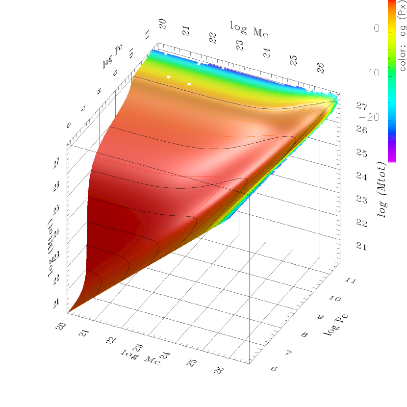
Figure 1: Manifold of proto-planet masses for a four day orbit around a solar type host star. The accretion parameter is set to $\dot{M}=10^{-4}\,\mathrm{M}_{\hbox{$\oplus$}}\,\mathrm{a}^{-1}$. The total proto-planet mass as a function of the parameters $M_{\mathrm{c}}$, $P_{\mathrm{c}}$. All axes are logarithmic. The results are connected to show a 3-dimensional surface. This surface is colored using the color-map shown in the upper right corner mapping the outside pressure $P_{\mathrm{x}}$ in a logarithmic way. This shows that the outside pressure is varied from $\approx 10^{4}to\approx 10^{-30}\,\mathrm{Pa}$. Everything with higher nebula pressures is by construction gravitationally unstable, lower pressures correspond to vacuum and cannot be calculated here properly because we do not calucate an atmosphere. This plot covers more than 6 magnitudes in $M_{\mathrm{c}}$ and $M_{\mathrm{tot}}$, and 5 magnitudes in $P_{\mathrm{c}}$.

2.2.2 Deriving the mass spectrum from a manifold

Having calculated a manifold, we now make the following assumptions:

1. All equilibria are equally probable.

2. All equilibria are stable and can be dynamically reached.

Now we can – quite in analogy to statistical mechanics – derive a distribution function for various properties of the proto-planets at that ”location”. The quantity we are interested in is the mass of the planet. By quite literally counting off the occuring masses in the manifold we can derive what we call the ”mass spectrum”: The relative frequency of planet masses at this location.

For this application of the manifold, it is important not to choose a certain range of core masses and core pressures implicitly by choice of a scale. Therefore, we chose a scale-free distribution to sample the parameter space in $M_{\mathrm{core}}$ and $P_{\mathrm{core}}$. In this way no core mass or core pressure is selected and all values are treated alike. The only scale-free distribution is a power-law distribution, or correspondingly a log-equidistant sampling of the parameter space. Obviously, if there were a dominant scale, e.g. in the core mass, this would drastically change the outcome as compared to our scale-free set-up.

The result for the same location as figure 1 is shown in figure 2. This mass spectrum is derived based on assumptions (i,ii). Therefore, either dynamical instability of some parts of the manifold, or quasistatic contraction with significant mass gain will change the observed mass spectrum. On the other hand, agreement of the mass spectra with observation would be a strong indication for the validity of the assumptions (i,ii).

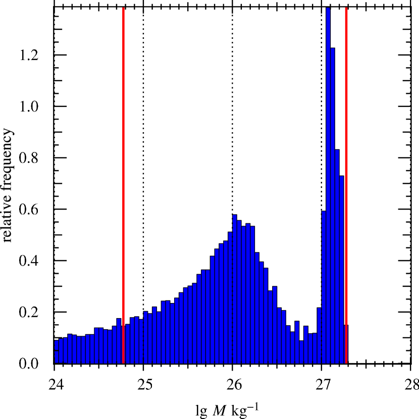
Figure 2: Mass spectrum of proto-planet masses for a four day orbit around a solar type host star. The accretion parameter is set to $\dot{M}=10^{-4}\,\mathrm{M}_{\hbox{$\oplus$}}\,\mathrm{a}^{-1}$. The area is normalized to 1. The red lines mark the value of 1 $\mathrm{M}_{\hbox{$\oplus$}}$ and 1 $\mathrm{M_{\jupiter}}$. The mass-distribution for 1 $\mathrm{M_{\astrosun}}$ at 4 d is clearly dominated by two peaks, one at $\approx 17\,\mathrm{M}_{\hbox{$\oplus$}}$ and another at $\approx 210\,\mathrm{M}_{\hbox{$\oplus$}}$ or $\approx 0.6\,\mathrm{M_{\jupiter}}$.

3 planet prediction results

3.1 Manifold survey

We have calculated manifolds and corresponding mass spectra for a wide range of locations by varying the following three parameters:

${(4)\,T_{\textrm{orb}}:}$

$1,\;4,\;16,\;64$ days

${(4)\,M_{\ast}:}$

$2,\;1,\;0.8,\;0.4\,\mathrm{M_{\astrosun}}$; $L_{\ast}=16,\;1,\;0.42,\;0.04\,\mathrm{L_{\astrosun}}$.

${(3)\,\dot{M}:}$

$10^{-2},\;10^{-4},\;10^{-6}\,\mathrm{M}_{\hbox{$\oplus$}}\,\textrm{a}^{-1}$.

This results in a 3-dimensional grid of locations, a total of 48 manifolds. This is the first complete survey of hydrostatic proto-planets in close orbits. The full set of results can be seen in Broeg (2006b) and is also available on-line at Broeg (2006a). This survey – named Corot survey Mark 1 v1.1 – revealed a large diversity of mass spectra in the range from 1 to 64 days orbital period. The host star mass also has large impact on the mass distributions.

3.2 Statistical properties – Three classes of gas giants

As stated in section 2.2.2 a manifold can be used to determine the mass spectrum using the following two hypotheses: 1) all equilibria are equally probable and 2) they can be dynamically reached, i.e. there exists a track from some set of initial conditions to each state. Using these hypotheses we can derive several interesting properties of the giant planets.

One major result of this survey is the fact that all mass spectra for close-in orbits exhibit two peaks. This is so for all tested values of $\dot{M}$. Moving to larger orbital distances, these peaks move closer together and eventually merge into one peak. For a solar type host star, this happens at an orbital period of around 16 days.

The full set of mass spectra of our survey leads to the grouping of the planets into three classes:

Class G

Extremely hot gas giants reside very close to the host star. Their surface temperature is above dust sublimation temperature. Planets in this class have a very large upper mass limit. For solar type host stars, the mass limit is roughly at 2.5 $\mathrm{M_{\jupiter}}$. For host stars of 2 $\mathrm{M_{\astrosun}}$, this limit is extended up to 6 $\mathrm{M_{\jupiter}}$. More massive planets should not exist this close to the star. In addition, we expect a very large quantity of so-called hot Neptunes with masses around 16 $\mathrm{M}_{\hbox{$\oplus$}}$ corresponding to a large second peak in the mass spectrum.

Class H

Hot gas giants reside in-between the classes G and J. Their surface temperature is below dust sublimation and they are close enough to their host star so that the mass spectra still show two distinct peaks. We expect them to be less massive than 1 $\mathrm{M_{\jupiter}}$ (for a 1 $\mathrm{M_{\astrosun}}$ host star).

Class J

Jupiter-like gas giants show only one peak in their mass spectrum. Class J planets can be much more massive than the classes G and H because the equilibria can gain significant amounts of mass by quasi-static contraction while the nebula is still present (see section 3.3).

For a solar type star, the boundaries between the groups G,H and H,J are at 4 days and 16 days orbital period, respectively.

3.3 Discussion

As discussed in the last section, the transition from class H to J is marked by the merger of the two peaks in the mass spectrum. We have performed both isothermal linear instability analysis (Schönke, J., 2005) and isothermal non-linear instability analysis (Pečnik, B., 2005) of a number of manifolds. These calculations suggest a fundamental change in dynamical properties that coincides (or is caused by) the merger of the peaks: In the one-peak case, entire regions in the manifold appear to be unstable owing to transitions between two states of similar mass.

Another change in behaviour at the merge position can be derived from the manifolds directly: At large orbital distances, there is a well-defined critical core mass beyond which no more static solutions exist inside a nebula. The value of the critical core mass depends only weakly on nebula pressure. This leads to the explanation why Jupiter and Saturn appear to have similar cores.

At small orbital distances, however, the critical core-mass becomes very strongly dependant on nebula pressure. In consequence, it is always possible to find a nebula pressure where the core is sub-critical, i.e. where a static solution exists. This renders the concept of a critical core mass meaningless for classes H and G. Following the above line of reasoning for close-in planets, it follows that no significant mass gain is expected by the disappearance of the nebula. Therefore the calculated mass spectrum of classes G and H could be very much like the observed mass spectrum in this regime.

These considerations have been tested in a small number of calculations using full radiation hydrodynamic planet formation. One such case is the planet HD 149026 b at a distance of 0.042 AU corresponding to an orbital period of 2.87 days. Our calculations show a completely hydrostatic evolution (see Broeg & Wuchterl, 2006) without significant mass gain in the final phase. The final planet has the same mass as the equilibrium configuration in the manifold.

3.4 First comparison with observations

Santos et al. (2005) detect a paucity of high-mass planetary companions with orbital periods shorter than $\sim 40$ days. This is in agreement with our separation in upper mass limit classes (G&H) and the J class without a strict upper mass limit.

Gaudi et al. (2005) went a step further dividing the observed exo-planets into very hot (VHJ) and hot Jupiters (HJ) with a dividing line at 3 days orbital period. They observe that the VHJ exhibit higher masses than the HJ; Specifically, the VHJ masses are larger than 1 $\mathrm{M_{\jupiter}}$. This is in perfect agreement with our separation into groups G & H and the upper mass limit of 1 $\mathrm{M_{\jupiter}}$ for group H.

As a final comparison of our method to observations we performed a direct ”prediction” for the host stars of today’s exo-planets. Because of the class properties, nameley the stability of equilibrium states for classes G & H and the lack thereof for the J class, we only compare our predicted masses at orbital periods less than 20 days. At the time of our analysis, 54 exo-planets fell in that regime. For the prediction we assumed all host stars to be solar. The reference mass spectrum was obtained by binning the masses of these 54 exo-planets in 0.3 dex mass bins. As most of the detected exo-planets have been observed using the radial velocity technique, we added a 30% correction to the observed planet masses as is statistically expected. This we compared to our theoretical mass spectrum: For each detected exo-planet we computed a mass spectrum using the corresponding orbital distance. All such mass spectra were added and binned according to the reference mass spectrum. The resulting mass spectrum is compared to the reference spectrum in figure 3. Please note that our calculated mass spectrum can only be expected to reproduce the observed one if there are no phases of quasi-static contraction while the nebula still exists, i.e. while there is a significant mass reservoir for the planet (this is the case for HD 149026b).

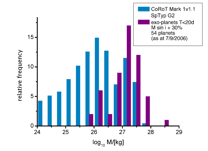
Figure 3: Predicted and observed mass distributions (Observed exo-planets from Schneider, 2006, on July 7, 2006). For this prediction we used only solar type host stars. The high-mass peak is in good agreement with the observed data. Only the very high data point is not reproduced but it might be a brown dwarf with a different formation mechanism. Including higher mass host stars would produce slightly higher upper masses in our prediction. The lower-mass peak of our calculations can already be noticed in the observed data but these planets are at the detection limits. We expect this part of the observed distribution to grow as the instruments become more sensitive. The high-mass end, on the other hand, should be complete for the observed stars.

4 Conclusion

We have presented a new method to predict the mass distribution of gas giant planets that analyses all possible hydrostatic equilibria. It has the advantage of not needing the nebula density as input. Only nebula temperature and planetesimal accretion rate must be known. In a passive disk, this can be easily approximated using the host star properties. This leaves the planetesimal accretion rate as the only free parameter.

Using our new method, we are able to split the giant planets into three classes G, H, and J which have distinct properties (see section 3.2). We compare these properties to the observed mass distribution of the exo-planets and find good agreement. We also produce a mass distribution for the exo-planet host stars having close-in planets and can reproduce the observed mass distribution. The agreement with observations is a strong argument that the equilibria are indeed dominating the formation process of close-in planets and that a large variety of proto-planetary nebulae is in existence.

To produce a prediction for COROT star fields, the existing mass spectra have to be averaged according to the distribution of stars in the COROT fields and a concept has to be developed to determine the relative planet abundance of planets at different orbital distances. So far we can only predict planetary mass distributions at given orbital distances.

References

- Alexander & Ferguson (1994) Alexander D. R., Ferguson J. W., 1994, ApJ, 437, 879
- Alibert et al. (2005a) Alibert Y., Mordasini C., Benz W., Winisdoerffer C., 2005a, A&A, 434, 343
- Alibert et al. (2005b) Alibert Y., Mousis O., Benz W., 2005b, ApJ, 622, L145
- Alibert et al. (2005c) Alibert Y., Mousis O., Mordasini C., Benz W., 2005c, ApJ, 626, L57
- Baglin & The COROT Team (1998) Baglin A., The COROT Team, 1998, in IAU Symp. 185: New Eyes to See Inside the Sun and Stars, Deubner F.-L., Christensen-Dalsgaard J., Kurtz D., eds., pp. 301–+
- Benz et al. (2006) Benz W., Mordasini C., Alibert Y., Naef D., 2006, in Tenth Anniversary of 51 Peg-b: Status of and prospects for hot Jupiter studies, Arnold L., Bouchy F., Moutou C., eds., pp. 24–34
- Bodenheimer & Pollack (1986) Bodenheimer P., Pollack J. B., 1986, Icarus, 67, 391
- Bordé et al. (2003) Bordé P., Rouan D., Léger A., 2003, A&A, 405, 1137
- Borucki & Summers (1984) Borucki W. J., Summers A. L., 1984, Icarus, 58, 121
- Boss (2002) Boss A. P., 2002, ApJ, 576, 462
- Broeg (2006a) Broeg C., 2006a, Corot survey, http://www.astro.uni-jena.de/corot/
- Broeg (2006b) —, 2006b, PhD thesis, Friedrich-Schiller-Universität Jena, Germany
- Broeg & Wuchterl (2006) Broeg C., Wuchterl G., 2006, The formation of hd 149026b, MNRAS, accepted 2007 Jan 9, astro-ph/0701340
- Charbonneau et al. (2000) Charbonneau D., Brown T. M., Latham D. W., Mayor M., 2000, ApJ, 529, L45
- COROT (2006) COROT, 2006, Corot, http://smsc.cnes.fr/COROT/
- Gaudi et al. (2005) Gaudi B. S., Seager S., Mallen-Ornelas G., 2005, ApJ, 623, 472
- Goldreich et al. (2004) Goldreich P., Lithwick Y., Sari R., 2004, ARA&A, 42, 549
- Götz (1989) Götz M., 1989, PhD thesis, Univ. Heidelberg
- Gray (1992) Gray D., 1992, The observation and analysis of stellar atmospheres, 2nd edn. Cambridge University Press, Cambridge
- Hayashi (1981) Hayashi C., 1981, Progress of Theoretical Physics Supplement, 70, 35
- Hayashi et al. (1977) Hayashi C., Nakazawa K., Adachi I., 1977, PASJ, 29, 163
- Hayashi et al. (1979) Hayashi C., Nakazawa K., Mizuno H., 1979, Earth and Planetary Science Letters, 43, 22
- Hayashi et al. (1985) Hayashi C., Nakazawa K., Nakagawa Y., 1985, in Protostars and Planets II, pp. 1100–1153
- Kippenhahn & Weigert (1990) Kippenhahn R., Weigert A., 1990, Stellar Structure and Evolution, Harwit M., Kippenhahn R., Trimble V., Zahn J.-P., eds., Astronomy and Astrophysics Library. Springer-Verlag, Berlin, Heidelberg
- Lissauer (1993) Lissauer J. J., 1993, ARA&A, 31, 129
- Mayor & Queloz (1995) Mayor M., Queloz D., 1995, Nature, 378, 355
- Mizuno (1980) Mizuno H., 1980, Progress of Theoretical Physics, 64, 544
- Pečnik & Wuchterl (2005) Pečnik B., Wuchterl G., 2005, A&A, 440, 1183
- Pečnik, B. (2005) Pečnik, B., 2005, Ph.d.thesis, Ludwig-Maximillians-Universität München, München, Germany
- Pollack et al. (1996) Pollack J. B., Hubickyj O., Bodenheimer P., Lissauer J. J., Podolak M., Greenzweig Y., 1996, Icarus, 124, 62
- Pollack et al. (1985) Pollack J. B., McKay C. P., Christofferson B. M., 1985, Icarus, 64, 471
- Rouan et al. (2000) Rouan D., Baglin A., Barge P., Bordé P., Deleuil M., Léger A., Schneider J., Vuillemin A., 2000, in ESA SP-451: Darwin and Astronomy : the Infrared Space Interferometer, Schürmann B., ed., pp. 221–+
- Santos et al. (2005) Santos N. C., Benz W., Mayor M., 2005, Science, 310, 251
- Saumon et al. (1995) Saumon D., Chabrier G., van Horn H. M., 1995, ApJS, 99, 713
- Schneider (2006) Schneider J., 2006, The extrasolar planets encyclopedia, http://exoplanet.eu/
- Schönke, J. (2005) Schönke, J., 2005, Diplomarbeit, Friedrich Schiller Universität Jena
- Weiss et al. (1990) Weiss A., Keady J. J., Magee N. H., 1990, Atomic Data and Nuclear Data Tables, 45, 209
- Wetherill & Stewart (1989) Wetherill G. W., Stewart G. R., 1989, Icarus, 77, 330
- Wuchterl (1990) Wuchterl G., 1990, A&A, 238, 83
- Wuchterl (1991a) —, 1991a, Icarus, 91, 39
- Wuchterl (1991b) —, 1991b, Icarus, 91, 53
- Wuchterl et al. (2000) Wuchterl G., Guillot T., Lissauer J. J., 2000, Protostars and Planets IV, 1081