Diffusion of Cosmic Rays in the Expanding Universe.
II. Energy Spectra of Ultra-High Energy Cosmic Rays

Abstract

We consider the astrophysical implications of the diffusion equation solution for Ultra-High Energy Cosmic Rays (UHECR) in the expanding universe, obtained in paper I (Berezinsky & Gazizov, 2006). The UHECR spectra are calculated in a model with sources located in vertices of the cubic grid with a linear constant (source separation) d. The calculations are performed for various magnetic field configurations ($B_{c},l_{c}$), where $l_{c}$ is the basic scale of the turbulence and $B_{c}$ is the coherent magnetic field on this scale. The main purpose of these calculations is to demonstrate the validity of the solution obtained in paper I and to compare this solution with the Syrovatsky solution used in previous works. The Syrovatsky solution must be necessarily embedded in the static cosmological model. The formal comparison of the two solutions with all parameters being fixed identically reveals the appreciable discrepancies between two spectra. These discrepancies are less if in both models the different sets of the best-fit parameters are used.

1 Introduction

Diffusive propagation of ultra-high energy cosmic rays (UHECR) in extragalactic space has been recently studied by Aloisio & Berezinsky (2004, 2005); Lemoine (2005); Aloisio et al. (2007a) using the Syrovatsky solution (see Syrovatskii (1959)) of the diffusion equation. This solution has been obtained under rather restrictive assumptions that diffusion coefficient $D(E)$ and energy losses $b(E)=-dE/dt$ of the propagating particles do not depend on time $t$. In our recent work (Berezinsky & Gazizov (2006), to be cited below as paper I) we found the analytic solution to the diffusion equation in the expanding universe, valid for the time-dependent diffusion coefficient $D(E,t)$ and energy losses $b(E,t)$. The aim of this work is to calculate spectra of UHE protons using the BG solution of paper I and to compare them with the spectra obtained with the help of the Syrovatsky solution in the above-cited papers.

The diffusion equation for ultra-relativistic particles propagating in the expanding universe from a single source, as obtained in paper I, reads

$$\frac{\partial n}{\partial t}-b(E,t)\frac{\partial n}{\partial E}+3H(t)n-n\frac{\partial b(E,t)}{\partial E}-\frac{D(E,t)}{a^{2}(t)}\ \mathbf{\nabla}_{x}^{2}n=\frac{Q_{s}(E,t)}{a^{3}(t)}\ \delta^{3}(\vec{x}-\vec{x}_{g}),$$ (1)

where the coordinate $\vec{x}$ corresponds to the comoving distance and $a(t)$ is the scaling factor of the expanding universe, $n=n(t,\vec{x},E)$ is the particle number density per unit energy in an expanding volume of the universe, $dE/dt=-b(E,t)$ describes the total energy losses, which include adiabatic $H(t)E$ and interaction $b_{int}(E,t)$ energy losses. $Q_{s}(E,t)$ is the generation function, that gives the number of particles generated by a single source at coordinate $\vec{x}_{g}$ per unit energy and unit time.

According to paper I, the spherically-symmetric solution of Eq. (1) is

$$n(x_{g},E)=\int_{0}^{z_{g}}dz\left|\frac{dt}{dz}(z)\right|\ Q_{s}[E_{g}(E,z),z]\ \frac{\exp[-x_{g}^{2}/4\lambda(E,z)]}{[4\pi\lambda(E,z)]^{3/2}}\ \frac{dE_{g}}{dE}(E,z),$$ (2)

where

$$\frac{dt}{dz}(z)=-\frac{1}{H_{0}\ (1+z)\sqrt{\Omega_{m}(1+z)^{3}+\Lambda}}$$ (3)

with cosmological parameters $\Omega_{m}=0.27$ and $\Lambda=0.73$,

$$\lambda(E,z)=\int_{0}^{z}dz^{\prime}\left|\frac{dt^{\prime}}{dz^{\prime}}\right|\ \frac{D(\mathcal{E}^{\prime},z^{\prime})}{a^{2}(z^{\prime})},$$ (4)

$$\frac{dE_{g}}{dE}(E,z)=(1+z)\exp\left[\int_{0}^{z}dz^{\prime}\left|\frac{dt^{\prime}}{dz^{\prime}}\right|\ \frac{\partial b_{int}(\mathcal{E}^{\prime},z^{\prime})}{\partial\mathcal{E}^{\prime}}\right].$$ (5)

The characteristic trajectory, $\mathcal{E}^{\prime}=E^{\prime}(E,z^{\prime})$, is a solution of the differential equation

$$\frac{dE}{dt}=-[H(t)E+b_{int}(E,t)].$$ (6)

It gives the energy $E^{\prime}$ of a particle at epoch $z^{\prime}$, if this energy is $E$ at $z=0$; we shall use also the notation $E_{g}(E,z)$ for this quantity. The upper limit $z_{g}$ in the integral of Eq. (2) is provided by maximum energy of acceleration as $E_{g}(E,z_{g})=E_{\rm max}$, or by $z_{\rm max}$ whichever is smaller.

To calculate the diffuse flux of UHE protons $J_{p}(E)$, we sum up contributions of sources located in the vertices of a 3D cubic lattice with spacing $d$. Positions of the sources $\vec{x}_{g}=(\xi,\eta,\zeta)$ are given by the coordinates $\xi=d(i+1/2)$, $\eta=d(j+1/2)$, $\zeta=d(k+1/2)$, where $i,j,k=0,\pm 1,\pm 2,..$ and position of the observer is assumed at $\xi=0,\eta=0,\zeta=0$. Thus we obtain

$$J_{p}(E)=\frac{c}{4\pi}\sum_{i,j,k}n(x_{ijk},E),$$ (7)

where $n(x_{ijk},E)$ is given by Eq. (2) and

$$x_{ijk}=d\sqrt{(i+1/2)^{2}+(j+1/2)^{2}+(k+1/2)^{2}}.$$ (8)

For the propagation of UHE protons in magnetic fields we follow the picture used by Aloisio & Berezinsky (2004, 2005), namely we assume the turbulent magnetized plasma. Magnetic field produced by turbulence is characterized by the value of the coherent magnetic field $B_{c}$ on the basic scale of turbulence $l_{c}$, which we shall keep in our estimates as $1$ Mpc. On the smaller scales $l<l_{c}$ the magnetic field is determined by the turbulence spectrum. The critical energy of propagation is determined by the relation $r_{L}(E_{c})=l_{c}$, where $r_{L}$ is the Larmor radius of a proton. Numerically, $E_{c}=0.93\times 10^{18}(B_{c}/1$ nG) eV. The characteristic propagation length in magnetic field is the diffusion length $l_{d}(E)$. It is defined as the distance on which a particle is deflected by 1 rad. The diffusion coefficient is defined as $D(E)=cl_{d}(E)/3$. For the case $r_{L}(E)\gg l_{c}$, i.e. when $E\gg E_{c}$, the diffusion length can be straightforwardly found from multiple scattering as

$$l_{d}(E)=1.2\ \frac{E^{2}_{18}}{B_{\rm nG}}~{}{\rm Mpc},$$ (9)

where $E_{18}=E/(10^{18}$ eV) and $B_{\rm nG}=B/(1$ nG). At $E=E_{c}$,  $l_{d}=l_{c}$.

At $E\ll E_{c}$ the diffusion length depends on the spectrum of turbulence. For the Kolmogorov spectrum $l_{d}(E)=l_{c}(E/E_{c})^{1/3}$; for the Bohm regime $l_{d}(E)=l_{c}\ (E/E_{c})$.

The strongest observational upper limit on the magnetic fields in our picture is given by Blasi, Burles & Olinto (1999) as $B_{c}\lesssim 6$ nG on the scale $l_{c}=50$ Mpc. In the calculations below we assume the representative values of $B_{c}$ in the range $(0.1-1)$ nG for $l_{c}=1$ Mpc.

We do not put as the aim of this paper the detailed study of diffusion in the time-dependent regime. Such a work (Aloisio et al., 2007b) is at present in progress. Here we want mainly to demonstrate the validity of the solution for expanding universe obtained in paper I and to perform the numerical comparison of the UHECR diffuse spectra predicted by BG and Syrovatsky solutions. The difference is expected to be substantial at energies $E\lesssim 3\times 10^{18}$ eV, where effects of the universe expansion (in particular, of the CMB temperature growth with red-shift) are not negligible. We want also to test the new solution obtained in paper I, namely to see the compatibility of the BG and Syrovatsky spectra at high energies, where the universe can be considered as the static one, as well as the convergence of BG spectra to the universal spectrum, when the source separation $d\rightarrow 0$.

The paper is organized as follows: Section 2 addresses the question how reliable is an assumption of the diffusion for the low-energy part of UHECR. In Section 3 we calculate the diffuse spectra using the time-dependent BG solution. In Section 4 we consider the static universe, which is the necessary assumption for the Syrovatsky solution, and in Section 5 we compare the spectra calculated for the expanding and static universes. The short conclusions are presented in Section 6.

2 Why diffusion?

We argue here that at least at the low-energy end of extragalactic UHECR the diffusion propagation is unavoidable for any reasonable magnetic field. We estimate also the magnetic field $B_{c}$ for which protons with energies $E\geq 10^{17}$ eV propagate quasi-rectilinearly, hence producing the same energy spectrum as in the case of rectilinear propagation.

To facilitate the calculations, let us consider the case of the static universe as in Aloisio & Berezinsky (2005), namely the universe with ’age’ $t_{0}=H_{0}^{-1}$, as follows from WMAP observations, and with fictitious ’adiabatic’ energy loss of particles $b(E)=E\,H_{0}$, where $H_{0}=72$ km/sMpc is the observed Hubble parameter.

In this picture there is a maximum diffusive distance – magnetic horizon – which is determined by the distance traversed by a particle during the age of the universe $t_{0}$:

$$r_{\rm hor}^{2}(E)=\int_{0}^{t_{0}}dt\ D[E_{g}(E,t)]\ ,$$ (10)

where $E_{g}(E,t)$ is the energy that a particle has at time $t$, if it is $E$ at $t=t_{0}$. Putting $dt=-dE_{g}/b(E_{g})$ in Eq. (10), we obtain

$$r_{\rm hor}^{2}(E)=\int_{E}^{E_{\rm max}}\frac{dE_{g}}{b(E_{g})}\ D(E_{g})\ ,$$ (11)

where $E_{\rm max}={\rm min}[E_{g}(E,t_{0}),E^{\rm acc}_{\rm max}]$.

In $r_{\rm hor}^{2}(E)$ one can recognize (see Aloisio & Berezinsky (2005)) the Syrovatsky variable $\lambda(E,E_{g})$ at $E_{g}=E_{\rm max}$ (for the physical discussion of magnetic horizon see Parizot (2004)).

Let us consider a transition from the diffusive to the rectilinear propagation, allowing the considerable deflection angle $\theta\gtrsim 1$, when the spectrum is the same as in the rectilinear propagation. Two conditions must be fulfilled:

$$r_{L}(E)>l_{c},$$ (12)

$$l_{d}(E)>r_{\rm hor}(E).$$ (13)

Eq. (12) gives a necessary (but not a sufficient!) condition: the scattering angle on a basic scale must be small enough, $\theta=l_{c}/r_{L}(E)<1$. It implies the propagation in the regime with $E>E_{c}$, where $l_{d}(E)=l_{c}\ (E/E_{c})^{2}$. Considering the low-energy case $E\leq 1\times 10^{18}$ eV, when the adiabatic energy loss dominates, so that $b(E)=EH_{0}$ and

$$E_{\rm max}=E_{g}(E,t_{0})=Ee^{H_{0}t_{0}}=eE,$$ (14)

one readily obtains from Eq (11)

$$r^{2}_{\rm hor}(E)=\frac{cl_{c}}{6H_{0}}\left(\frac{E}{E_{c}}\right)^{2}(e^{2}-1).$$ (15)

Using Eq. (13) we get

$$\frac{E_{c}}{E}\leq\left[\frac{cH_{0}^{-1}}{6l_{c}}(e^{2}-1)\right]^{-1/2}.$$ (16)

From $r_{L}(E_{c})=l_{c}$ we obtain $E_{c}=qB_{c}l_{c}$, where $q$ is an electric charge, which equals $300$ for a proton, if $B$ is measured in Gauss and $E$ in eV.

Finally we have

$$B_{c}\leq\frac{E}{ql_{c}}\left[\frac{cH_{0}^{-1}}{6l_{c}}(e^{2}-1)\right]^{-1/2},$$ (17)

or, numerically,

$$B_{c}\leq 1.6\times 10^{-3}\ \frac{E}{10^{17}~{}{\rm eV}}\left(\frac{l_{c}}{1~{}{\rm Mpc}}\right)^{-1/2}~{}{\rm nG}.$$ (18)

Therefore, $B_{c}\leq 1.6\times 10^{-3}$ nG provides the quasi-rectilinear propagation for all protons with energies $E\geq 1\times 10^{17}$ eV, while at lower energies the diffusion description is applicable. For the reasonably low field $B_{c}\approx 0.01$ nG the diffusion becomes valid at $E\lesssim 1\times 10^{18}$ eV.

3 Diffusive energy spectra of UHECR in the expanding universe

In the following calculations we shall use the simplified illustrative description of magnetic field evolution with redshift, namely we parametrize the evolution of magnetic configuration $(l_{c},B_{c})$ as

$$l_{c}(z)=l_{c}/(1+z),\ \ \ B_{c}(z)=B_{c}\ (1+z)^{2-m},$$

where factor $(1+z)^{2}$ describes the diminishing of the magnetic field with time due to magnetic flux conservation and $(1+z)^{-m}$  – due to MHD amplification of the field. The critical energy $E_{c}(z)$ found from $r_{L}(E)=l_{c}(z)$ is given by

$$E_{c}(z)=0.93\times 10^{18}\ (1+z)^{1-m}\ \frac{B_{c}}{1~{}\mbox{nG}}$$

for $l_{c}=1$ Mpc. The maximum redshift used in the calculations is $z_{\rm max}=4$.

The diffuse flux is calculated for the lattice distribution of the sources (in the coordinate space $\vec{x}$) with lattice parameter (the source separation) $d$ and a power-law generation function for a single source

$$Q_{s}(E)=\frac{q_{0}(\gamma_{g}-2)}{E_{0}^{2}}\left(\frac{E}{E_{0}}\right)^{-\gamma_{g}},$$ (19)

where $E_{0}$ is the normalizing energy, for which we will use $1\times 10^{18}$ eV and $q_{0}$ has a physical meaning of a source luminosity in protons with energies $E\geq E_{0}$, $L_{p}(\geq E_{0})$. The corresponding emissivity $\mathcal{L}_{0}=q_{0}/d^{3}$, i.e. the energy production rate in particles with $E\geq E_{0}$ per unit comoving volume, will be used to fit the observed spectrum by the calculated one.

Using to Eqs. (2–8), one obtains the diffuse spectrum as

$$J_{p}(E) = \frac{c}{4\pi H_{0}}\ \frac{q_{0}(\gamma_{g}-2)}{E_{0}^{2}}\times$$ (20)

$$\sum_{i}\int\limits_{0}^{z_{g}}dz\frac{\left[E_{g}(E,z)/E_{0}\right]^{-\gamma_{g}}}{(1+z)\sqrt{\Omega_{m}(1+z)^{3}+\Lambda}}\ \frac{\exp[-\frac{x_{i}^{2}}{4\lambda(E,z)}]}{[4\pi\lambda(E,z)]^{3/2}}\ \frac{dE_{g}(E,z)}{dE},$$

where summation goes over the sources like in Eqs. (7) and (8), the upper limit $z_{g}$ is provided by maximum energy of acceleration as $E_{g}(E,z_{g})=E_{\rm max}^{\rm acc}$ or by $z_{\rm max}$, whichever is smaller, $\gamma_{g}$ is the generation index and a formula for $dE_{g}/dE$ can be found in Berezinsky & Grigorieva (1988) and Berezinsky et al. (2002a). The analogue of the Syrovatsky variable, $\lambda(E,z)$, is given by

$$\lambda(E,z)=\frac{1}{H_{0}}\int_{0}^{z}dz\frac{(1+z)}{\sqrt{\Omega_{m}(1+z)^{3}+\Lambda}}\ D[E_{g}(E,z),z].$$ (21)

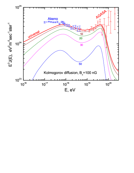
Figure 1: Convergence of the diffusive solution (7) to the universal spectrum when the distance between sources diminishes from 50 to 10 Mpc shown by numbers on the curves. The magnetic field configuration $(B_{c},l_{c})=(100$ nG, 1 Mpc) with the Kolmogorov spectrum of turbulence. The emissivity $\mathcal{L}_{0}=q_{0}/d^{3}=2.4\times 10^{45}$ erg/Mpc³yr is the same for all curves. The generation spectrum is $\propto E^{-2.7}$. The spectrum of Akeno-AGASA (Honda et al., 1993; Shinozaki, 2006) is shown for comparison.

First of all we test the correctness of the obtained solution with the help of propagation theorem (Aloisio & Berezinsky, 2004), which states that diffusive solution (7) converges to the universal spectrum, i.e. one calculated for homogeneous source distribution (see Berezinsky et al. (2002a)) when the distances between sources $d\rightarrow 0$. Fig. 1 demonstrates this convergence for the case of strong magnetic field, $B_{c}=100$ nG, and the Kolmogorov diffusion at $E<E_{c}$. The diffuse fluxes are calculated using Eq. (7) for $d$ diminishing from $50$ Mpc to $10$ Mpc, keeping the same comoving volume emissivity $\mathcal{L}_{0}=q_{0}/d^{3}=2.4\times 10^{45}$ erg/Mpc³yr. The generation spectrum is given by $\gamma_{g}=2.7$. One can observe the convergence of the calculated spectra to the universal one when $d\rightarrow 0$, in accordance with propagation theorem.

For small distances between a source and observer, the diffusion approximation for a particle propagation is not valid. One can see it from a simple argument that diffusive propagation time $r^{2}/D$ must be larger than time of rectilinear propagation, $r/c$. This condition, using $D\sim c\,l_{d}$, results in $r\lesssim l_{d}$. At distances $r\lesssim l_{d}$ the rectilinear and diffusive trajectories in magnetic fields differ but little and rectilinear propagation is a good approximation as far as spectra are concerned. The number densities of particles $Q/4\pi cr^{2}$ and $Q/4\pi Dr$, calculated in rectilinear and diffusive approximations, respectively, are equal at $r\sim l_{d}$, where $Q$ is the rate of particle production by a source. At smaller distances the rectilinear flux dominates, at larger – the diffusive one. We calculated the number densities of protons $n(E,r)$ numerically for both modes of propagations with energy losses of protons taken into account, and the distance of transition is taken from equality of the calculated densities. We know that this recipe is somewhat rough and the interpolation between two regimes is required, as in calculations by Aloisio & Berezinsky (2005). However any interpolation meets the difficulties by the following reason.

In fact, the diffusive regime sets up at distances not less than six diffusion lengths $l_{d}$. At distances $l_{d}\lesssim r\lesssim 6\,l_{d}$ some intermediate regime of propagation in magnetic fields is valid. When studied in numerical simulations (e.g. Yoshiguchi (2003)), the calculated number density $n(E,r)$ satisfies the particle number conservation $4\pi r^{2}nu=Q$, where $u$ is the streaming velocity, while in case of interpolation there is only one (unknown) interpolation $n(E,r)$ which conserves the number of particles. This problem will be studied in detail in (Aloisio et al., 2007b), while for purposes of this paper we can accept the rough recipe of transition from diffusive to rectilinear regime as described above. The appearance of the artificial peculiarity connected with the accepted propagation transition will be useful serving as a mark for the position of transition in the spectrum.

For rectilinear propagation for the lattice distribution of the sources the diffuse spectrum is calculated as (Berezinsky et al., 2002a)

$$J_{p}(E) = \frac{(\gamma_{g}-2){\cal L}_{0}d}{(4\pi)^{2}E_{0}^{2}}\times$$ (22)

$$\sum\limits_{i,j,k}\frac{\left[E_{g}(E,z_{ijk})/E_{0}\right]^{-\gamma_{g}}}{[(i+1/2)^{2}+(j+1/2)^{2}+(k+1/2)^{2}](1+z_{ijk})}\ \frac{dE_{g}}{dE}(E,z_{ijk}),$$

where $\mathcal{L}_{0}=q_{0}/d^{3}=2.4\times 10^{45}$ erg/(Mpc³yr) is the emissivity, $z_{ijk}$ is the red-shift for a source with coordinates $i,j,k$, and factor $(1+z_{ijk})$ takes into account the time dilation.

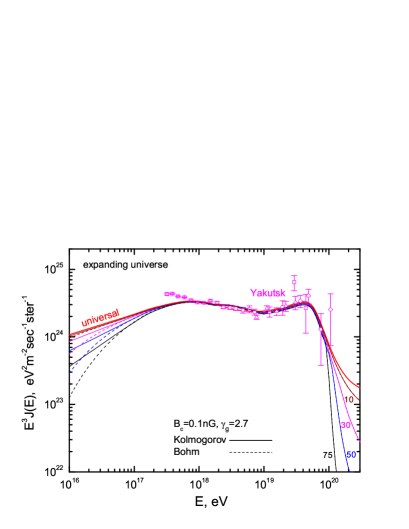
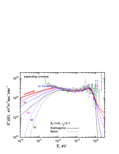
Figure 2: Diffusive spectra in the expanding universe for $B_{c}=0.1$ nG (left panel) compared with Yakutsk data (Egorova et al., 2004) and $B_{c}=1$ nG (right panel) compared with all-data Akeno-AGASA-HiRes-Yakutsk spectrum (Honda et al., 1993; Shinozaki, 2006; Abbasi et al., 2004; Egorova et al., 2004). The spectra are calculated as a combination of diffusive and rectilinear spectra with the Kolmogorov (solid lines) and Bohm (dash lines) regimes of diffusion at low energies $E<E_{c}$. The numbers at the curves indicate the separations of the sources in Mpc. The spectral generation index $\gamma_{g}=2.7$ and maximum acceleration energy $E_{\rm max}=1\times 10^{22}$ eV.

The calculated spectra in the expanding universe for $B_{c}=1$ nG and $B_{c}=0.1$ nG, both for $m=1$ and $E_{\rm max}=1\times 10^{22}$ eV are shown in Fig. 2 in comparison with all data (left panel) and Yakutsk data (Egorova et al., 2004) (right panel). The all-data spectrum is obtained using the of energy calibration of all detectors with help of the dip (Berezinsky et al., 2002a). One can observe the peculiarity in predicted spectrum in the right panel ($B_{c}=1$ nG) at energy $E\approx 2\times 10^{19}$ eV. This is the energy of transition to rectilinear propagation. This peculiarity is unphysical and is connected with the simplified description of the transition as described above. When magnetic field diminishes a peculiarity shifts toward lower energy (left panel) as it should do. At small $d$ the calculated spectra converge to the universal spectrum, as it must be.

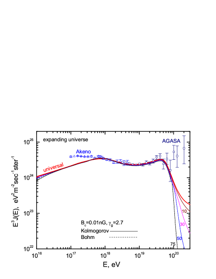
Figure 3: The same as in Fig. 2, but for $B_{c}=0.01$ nG and Akeno-AGASA (Honda et al., 1993; Shinozaki, 2006) data.

The spectra for very low magnetic field with $B_{c}=0.01$ nG is shown in Fig. 3. One can notice that the peculiarity is shifted here to the energy $E\sim 2\times 10^{17}$ eV and above this energy the spectrum is rectilinear. This behavior corresponds to the discussion in Section 2.

4 Spectra in the static universe

In this section we study the Syrovatsky solution of UHECR diffusion equation with aim of comparing it with the BG solution for the expanding universe. The Syrovatsky solution is valid in case of infinite space with time-independent diffusion coefficient $D(E)$ and energy losses $b(E)$. This implies the static universe.

We define the static universe in which the stationary diffusion equation with the Syrovatsky solution is embedded in the following way. There is no expansion. The Hubble constant is assumed as a formal parameter $H_{0}=72$ km/s Mpc, which defines the ”age” $t_{0}$ of the universe according to WMAP relation $H_{0}t_{0}=0.993$, so that $ct_{0}$ is the size of the universe: the space density of the UHECR sources outside the sphere of radius $ct_{0}$ is $n_{s}=0$. The temperature of CMB photons is constant, $T_{0}=2.728$ K, and thus the interaction energy losses $dE/dt=-b(E)$ are time-independent.

Apart from interaction energy losses, we assume the fictitious adiabatic energy losses described by $dE/dt=-H_{0}E$. In this approach we follow the work by Aloisio & Berezinsky (2005).

The universal spectrum in the static universe is different from that in the expanding universe. It is defined in the same way as in the expanding universe (Berezinsky et al., 2002a), namely from the number of particles conservation

$$n_{\rm univ}(E)=\int^{t_{0}}_{0}dt\,Q_{\rm gen}[E_{g}(E,t)]\,\frac{dE_{g}}{dE},$$ (23)

where $Q_{\rm gen}(E_{g})$ is the generation rate per unit volume and $E_{g}(E,t)$ is determined by the evolution equation $dE/dt=-b(E)$. Note that in the expanding universe $Q_{\rm gen}(E,t)$ and $n(E,t)$ are related to a comoving volume. In contrast to the expanding universe, the ratio $dE_{g}/dE$ in Eq. (23) is given by a simple expression (Berezinsky & Grigorieva, 1988) $dE_{g}/dE=b(E_{g})/b(E)$. Using

$$Q_{\rm gen}(E_{g})=\frac{(\gamma_{g}-2)\mathcal{L}_{0}}{E_{0}^{2}}\left(\frac{E_{g}}{E_{0}}\right)^{-\gamma_{g}},$$ (24)

where $\mathcal{L}_{0}$ is the emissivity in particles with energies $E\geq E_{0}$ for spectral index $\gamma_{g}>2$, one easily obtains the universal spectrum in analytic form:

$$n_{\rm univ}(E)=\frac{\gamma_{g}-2}{\gamma_{g}-1}\ \frac{\mathcal{L}_{0}}{E_{0}^{2}}\ \frac{\left(E/E_{0}\right)^{-\gamma_{g}}}{E^{-1}b(E)}\left[1-\left(\frac{E}{E_{\rm max}}\right)^{\gamma_{g}-1}\right],$$ (25)

where $E_{\rm max}={\rm min}[E_{g}(E,t_{0}),E_{\rm max}^{\rm acc}]$. For the diffuse spectra calculations we use the lattice distribution of the sources like in the previous section, with the same procedure of transition from diffusive to rectilinear propagation, but using for diffusive propagation the Syrovatsky solution (see also Aloisio & Berezinsky (2005)), instead of the BG solution.

In Fig. 4 we present the diffuse UHECR spectra calculated, like in Section 3, in the grid model with spacing $d$. UHECR sources are located in vertices of the grid. The spectra are calculated as combination of the diffusive flux, described by the Syrovatsky solution, combined with the rectilinear flux. They are presented for two magnetic field configurations $(B_{c},l_{c})$ equal to $(1\mbox{~{}nG},1\mbox{~{}Mpc})$ and $(0.1\mbox{~{}nG},1\mbox{~{}Mpc})$ and for different spacings $d$ indicated by the numbers in Mpc at the corresponding curves. Like in Section 3, the spectra have irregularities at energy of transition from diffusive to rectilinear propagation, caused by the rough method of sewing together of the two propagation regimes.

The calculated diffuse fluxes converge to the universal spectrum (25) when $d\rightarrow 0$, as it should be according to propagation theorem. In contrast to calculations by Aloisio & Berezinsky (2005), we have obtained the best fit of the data using $\gamma_{g}=2.65$, which is insignificantly different from $\gamma_{g}=2.7$ of (Aloisio & Berezinsky, 2005). One can see the basic agreement of these spectra with those in the expanding universe, including spectrum peculiarities caused by transition from diffusive to rectilinear propagation.

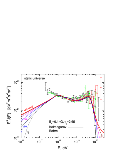
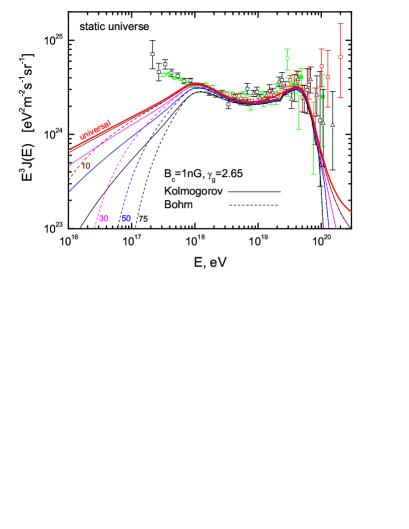
Figure 4: Diffuse spectra in the static universe for $B_{c}=0.1$ nG (left panel) and $B_{c}=1$ nG (right panel). The spectra are calculated as combination of diffusive and rectilinear spectra with the Kolmogorov (solid lines) and Bohm (dash lines) regimes of diffusion at low energies $E<E_{c}$. The numbers at the curves indicate the separation of the sources in Mpc. Observational data are the same as in the right panel of Fig. 2.

5 Comparison of spectra in expanding and static universes

The direct comparison of the BG and Syrovatsky solutions of diffusion equations is not possible because they are embedded in the different cosmological environments. While the BG solution is valid for the expanding universe, the Syrovatsky solution is valid only for the static universe. Using two different cosmological models for these solutions, there are two ways of comparison.

The first one is given by equal values of parameters in both solutions. In this method for BG solution we use the standard cosmological parameters for expanding universe $H_{0}$, $\Omega_{m}$, $\Lambda$ and maximum red-shift $z_{max}$ up to which UHECR sources are still active, magnetic field configuration ($B_{c},l_{c}$), separation $d$ and UHECR parameters $\gamma_{g}$ and $\mathcal{L}_{0}$, determined by the best fit of the observed spectrum. For the static universe with the Syrovatsky solution we use the same parameters $H_{0}$, $d$, ($B_{c},l_{c}$), $\gamma_{g}$ and $\mathcal{L}_{0}$. The maximum red-shift in the BG solution we chose as that providing the age of universe which equals to $t_{0}=H_{0}^{-1}$ in the static universe ($z_{max}=1.465$). This formal method of comparison will be referred to as ”equal-parameter method”.

Physically better justified comparison is given by the best fit method, in which $\gamma_{g}$ and $\mathcal{L}_{0}$ are chosen as the best fit parameters for the both solutions, respectively. As a matter of fact, we would use the best-fit parameters $\gamma_{g}$ and $\mathcal{L}_{0}$ for each solution, if we considered them independently. The weakness of this method is a ”forced” agreement at the energy range of measured UHECR spectrum, provided by the best-fit parameters to the same spectrum. Then the difference of the two solutions becomes most appreciable at $E\leq 1\times 10^{18}$ eV.

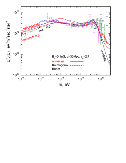
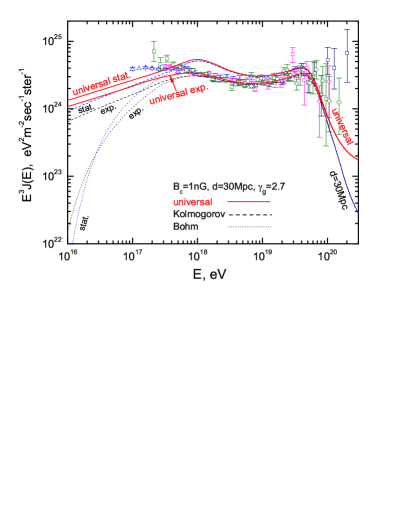
Figure 5: Equal-parameter comparison of the expanding (exp.) and static (stat.) universe solutions for $\gamma_{g}=2.7$, $\mathcal{L}_{0}=2.4\times 10^{45}$ erg/Mpc³yr and $d=30$ Mpc. The left panel shows the case $B_{c}=0.1$ nG, the right panel is for $B_{c}=1$ nG. The universal spectra are shown by solid lines. The cases of the Kolmogorov and Bohm diffusion at $E<E_{c}$ are shown by dash and dot lines, respectively. Data in both panels are the same as in the right panel of Fig. 2.

Equal-parameter comparison of the expanding and static universe solutions are shown in Fig. 5 for $\gamma_{g}=2.7$, $\mathcal{L}_{0}=2.4\times 10^{45}$ erg/Mpc³yr and $d=30$ Mpc. In the left panel $B_{c}=0.1$ nG and in the right panel $B_{c}=1$ nG. The universal spectra for the expanding and static universes are shown by solid lines. The Kolmogorov diffusion at $E<E_{c}$ is presented by dash lines and the Bohm diffusion – by dot lines. Note that universal spectra are different at $E<1\times 10^{19}$ eV as they must be due to excessive energy losses in the expanding universe caused by the increasing of CMB temperature $T(z)$ with red-shift. At the highest energy end $E\gtrsim 6\times 10^{19}$ eV the two solutions coincide exactly because at these energies the energy-attenuation time is short, the CMB temperature does not change during time-of-flight and the expanding universe case becomes static. As one can see in Fig. 5, at these energies both universal spectra are the same and all spectra for $d=30$ Mpc merge into one curve. The difference of fluxes at lower energies is naturally explained by the increase of energy losses in the expanding universe because of $T_{CMB}(z)$ dependence, and due to cosmological evolution of the magnetic field.

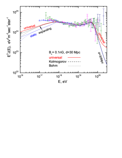
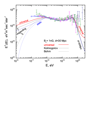
Figure 6: Best fit comparison of the expanding and static universe solutions for $d=30$ Mpc. Best-fit parameters are $\gamma_{g}=2.7,\mathcal{L}_{0}=2.4\times 10^{45}\ \mbox{erg}/\mbox{Mpc}^{3}\mbox{yr})$ for expanding and $\gamma_{g}=2.65,\mathcal{L}_{0}=5.7\times 10^{44}\ \mbox{erg}/\mbox{Mpc}^{3}\mbox{yr})$ for static solutions, respectively. The universal spectrum is shown for the expanding universe. The left panel exposes the case of $B_{c}=0.1$ nG and the right one the case of $B_{c}=1$ nG. The combined data of all arrays are shown for comparison. Data in both panels are the same as in the right panel of Fig. 2.

The best-fit comparison of the expanding and static universe solutions is shown in Fig. 6. The best-fit parameters are $(\gamma_{g}=2.7,\mathcal{L}_{0}=2.4\times 10^{45}\ \mbox{erg}/\mbox{Mpc}^{3}\mbox{yr})$ and $(\gamma_{g}=2.65,\mathcal{L}_{0}=5.7\times 10^{44}\ \mbox{erg}/\mbox{Mpc}^{3}\mbox{yr})$ for the expanding and static universes, respectively. The left panel shows the case $B_{c}=0.1$ nG and the right panel $B_{c}=1$ nG, both for $d=30$ Mpc. One can see a good (though ”forced”) agreement between the expanding universe and static universe solutions in the energy range of UHECR observations, which is improved in comparison with equal-parameter method because of the choice of the best-fit parameters $(\gamma_{g},\mathcal{L}_{0})$ different for each case.

However, we emphasize again that this is a natural way of selection of the solution in independent analysis. At energies below $1\times 10^{18}$ eV the larger discrepancies are seen, being induced by larger energy losses and evolution of magnetic field in case of expanding universe.

In conclusion, one can see a reasonably good agreement between the Syrovatsky solution, embedded in static universe model, with the BG solution for expanding universe at energies $E>1\times 10^{18}$ eV with noticeable discrepancies at smaller energies, which are natural and understandable.

6 Conclusions

In this paper we study the application of solution of diffusion equation in expanding universe obtained in the paper I to the propagation of UHE protons. However, we do not consider here the detailed picture with realistic evolution of magnetic field in expanding universe, and with a realistic transition from the diffusive to the quasi-rectilinear propagation. It is to be considered in our next work Aloisio et al. (2007b).

In this paper we demonstrate that solution of diffusion equation found in paper I looks quite reasonable when applied to realistic models. Numerically these solutions are similar to the Syrovatsky solutions valid for the static universe with the understandable distinctions at low energies.

The diffusion spectra in expanding universe are presented in Figs. 1, 2, 3 for the following magnetic configurations $(B_{c},l_{c})=(100\mbox{~{}nG},1\mbox{~{}Mpc})$, $(1\mbox{~{}nG},1\mbox{~{}Mpc})$, $(0.1\mbox{~{}nG},1\mbox{~{}Mpc})$ and $(0.01\mbox{~{}nG},1\mbox{~{}Mpc})$, respectively. In the latter case the energy spectra at $E>1\times 10^{17}$ eV are practically the same as in the case of rectilinear propagation. The evolution of magnetic field in the expanding universe is given by one illustrative example. The spectra are shown for different separations $d$ of the sources. Transition from diffusive to rectilinear propagation is described by the simplified recipe, which results in the artificial spectral features as described in Section 3. The best fit of the observed spectrum needs the same index of generation spectrum $\gamma_{g}=2.7$ as in the case of universal spectrum. The diffusive spectrum converges to universal spectrum when $d\rightarrow 0$, as it should be according to the propagation theorem.

The Syrovatsky solution of the diffusion equation, i.e. one when the diffusion coefficient $D(E)$ and energy losses $dE/dt=-b(E)$ do not depend on time $t$, is valid only for the static universe. In the static universe we make several additional assumptions. We introduce the Hubble constant $H_{0}$ as a formal parameter, which determines the fictitious ”adiabatic” energy losses $dE/dt=-EH_{0}$. The ”age” of the universe $t_{0}=H_{0}^{-1}$ determines fact the sphere of radius $r_{0}=ct_{0}$ occupied by the sources. For this universe we calculate the universal spectrum given by Eq. (25) and the diffusive spectra for given magnetic configuration $(B_{c},l_{c})$ and different separations of the sources $d$. The convergence to the universal spectrum occurs when $d\rightarrow 0$ as it should be. The best fit of the observational data is obtained when $\gamma_{g}=2.65$, which can be considered as a good agreement with the work by Aloisio & Berezinsky (2004), where $\gamma_{g}=2.7$ was used.

For the comparison of the BG and Syrovatsky solutions we use two schemes. In the formal one we compare the BG and Syrovatsky solutions for the same magnetic configurations $(B_{c},l_{c})$ and the same emissivities $\mathcal{L}_{0}$. One can see from Fig. 5 that both solutions coincide exactly at $E\geq 6\times 10^{19}$ eV, when effect of universe expansion (most notably variation of CMB temperature) can be neglected. At lower energies the difference in the spectra naturally emerges due to $T_{CMB}(t)$ dependence and thus due to different energy losses in the two solutions. Since the energy losses in the expanding universe are larger, the BG spectra occur below the Syrovatsky spectra.

For practical applications the discrepancy in the spectra at energy range $1\times 10^{18}-5\times 10^{19}$ eV is not essential, because it is eliminated by renormalization of the calculated flux, i.e. by changing the emissivity $\mathcal{L}_{0}$ for the static universe solution. In fact, this procedure is necessary for fitting of the observed spectra.

The comparison of two solutions as given above is formal. As was emphasized above, the Syrovatsky solution, which is valid for infinite space and time, with time-independent $D(E)$ and $b(E)$, needs the specific definition of the static universe. Only in this case one obtains the physically viable solution. This solution needs the best fit parameters $\gamma_{g}$ and $\mathcal{L}_{0}$, which are different from those in expanding universe. It is physically more meaningful to compare the spectra using for static universe its own best fit parameters $\gamma_{g}$ and $\mathcal{L}_{0}$ different from that in the expanding universe. The comparison shown in Figs. 6 reveals less discrepancies than in the formal scheme of comparison.

7 Acknowledgments

We are grateful to Vitaly Kudryavtsev for valuable discussions and participation in a part of this work. This work has been supported by TA-DUSL activity of the ILIAS program (contract No. RII3-CT-2004-506222) as part of the EU FP6 programme.

References

- Abbasi et al. (2004) Abbasi, R.U. et al., [HiRes Collaboration] 2004, Phys. Rev. Lett., 92, 151101
- Aloisio & Berezinsky (2004) Aloisio, R., & Berezinsky, V. 2004, ApJ, 612, 900
- Aloisio & Berezinsky (2005) Aloisio, R., & Berezinsky, V. 2005, ApJ, 625, 249
- Aloisio et al. (2007a) Aloisio, R., Berezinsky, V., Blasi, P., Gazizov, A., Grigorieva, S., & Hnatyk, B. 2007a, Astropart. Phys., 27, 76
- Aloisio et al. (2007b) Aloisio, R., Berezinsky, V., & Gazizov A.Z. 2007b, in progress
- Berezinsky & Grigorieva (1988) Berezinsky, V.S., & Grigorieva, S.I. 1988, A&A, 199, 1
- Berezinsky et al. (1990) Berezinsky, V.S., Bulanov, S.V., Dogiel, V.A., Ginzburg, V.L., & Ptuskin, V.S. 1990, Astrophysics of Cosmic Rays, North-Holland.
- Berezinsky et al. (2002a) Berezinsky, V., Gazizov, A.Z., & Grigorieva, S.I. 2002a, Phys. Rev. D, 74, 043005; [hep-ph/0204357 v1]
- Berezinsky et al. (2002b) Berezinsky, V., Gazizov, A.Z., & Grigorieva, S.I. 2002b, astro-ph/0210095
- Berezinsky & Gazizov (2006) Berezinsky, V., & Gazizov, A.Z. 2006, ApJ, 643, 8
- Blasi, Burles & Olinto (1999) Blasi, P., Burles, S. & Olinto, A. 1999 ApJ, 514, L79
- Egorova et al. (2004) Egorova, V.P., et al., [Yakutsk Collaboration] 2004, Nucl. Phys. B (Proc. Suppl.), 136, 3
- Honda et al. (1993) Honda, M., et al., [Akeno Collaboration] 1993, Phys. Rev. D, 70, 525
- Lemoine (2005) Lemoine, M. 2005, Phys. Rev. D, 71, 083007
- Parizot (2004) Parizot, E. 2004, Nucl. Phys. B (Proc. Suppl.) 136, 169
- Shinozaki (2006) Shinozaki, K., [AGASA Collaboration] 2006, Nucl. Phys. B (Proc. Suppl.), 151, 3
- Syrovatskii (1959) Syrovatskii, S.I. 1959, Sov. Astron. J., 3, 22 [1959, Astron. Zh., 36, 17]
- Yoshiguchi (2003) Yoshiguchi, H., Nagataki, S., Tsubaki, S. & Sato, K. 2003, ApJ, 586, 1211