A Census of Intrinsic Narrow Absorption Lines in the Spectra of Quasars at $z=2$–4

Abstract

We use Keck/HIRES spectra of 37 optically bright quasars at $z=2$–4 to study narrow absorption lines that are intrinsic to the quasars (intrinsic NALs, produced in gas that is physically associated with the quasar central engine). We identify 150 NAL systems, that contain 124 C IV, 12 N V, and 50 Si IV doublets, of which 18 are associated systems (within 5,000 km s^-1 of the quasar redshift). We use partial coverage analysis to separate intrinsic NALs from NALs produced in cosmologically intervening structures. We find 39 candidate intrinsic systems, (28 reliable determinations and 11 that are possibly intrinsic). We estimate that 10–17% of C IV systems at blueshifts of 5,000–70,000 km s^-1 relative to quasars are intrinsic. At least 32% of quasars contain one or more intrinsic C IV NALs. Considering N V and Si IV doublets showing partial coverage as well, at least 50% of quasars host intrinsic NALs. This result constrains the solid angle subtended by the absorbers to the background source(s). We identify two families of intrinsic NAL systems, those with strong N V absorption, and those with negligible absorption in N V, but with partial coverage in the C IV doublet. We discuss the idea that these two families represent different regions or conditions in accretion disk winds. Of the 26 intrinsic C IV NAL systems, 13 have detectable low-ionization absorption lines at similar velocities, suggesting that these are two-phase structures in the wind rather than absorbers in the host galaxy. We also compare possible models for quasar outflows, including radiatively accelerated disk-driven winds, magnetocentrifugally accelerated winds, and pressure-driven winds, and we discuss ways of distinguishing between these models observationally.

1 Introduction

Quasars and active galactic nuclei (AGNs) are thought to be powered by accretion of matter onto a supermassive black hole. The accretion flow onto the black hole is thought to proceed via an equatorial accretion disk, which provides a mechanism for removing the angular momentum of the infalling matter. Outflows (winds) from such disks appear to be an inseparable part of this process. More specifically, hydromagnetic winds (e.g., Blandford & Payne 1982; Emmering, Blandford & Shlosman 1992; Konigl & Kartje 1994; Everett 2005) provide a potential mechanism for extracting angular momentum from the accreting material, thus allowing accretion to proceed. Accretion disk winds are likely to be responsible for the broad absorption lines (BALs) observed in the spectra of a fraction of quasars (e.g., Murray et al. 1995; Arav, Li, & Begelman 1994, Proga, Stone, & Kallman 2000) and may even be the source of the broad emission lines that are the hallmark of all quasars and AGNs (e.g., Chiang & Murray 1996; Murray & Chiang 1997). Understanding the quasar outflow mechanisms by testing and refining theoretical models is therefore an essential part of our quest to understand the central engines of AGNs and quasars.

Quasar outflows also have quite important consequences for cosmology and galaxy formation and evolution because they provide energy and momentum feedback to the interstellar medium (ISM) of the host galaxy and to the intergalactic medium (IGM). Simulations of galaxy evolution through mergers (Springel, Di Matteo & Hernquist 2005) show that AGN feedback heats the ISM and inhibits star formation. Thus the colors of the resulting galaxies evolve very quickly to the red, in agreement with the observed color distribution of nearby galaxies. In semi-analytic models of galaxy assembly (Granato et al. 2004; Scannapieco & Oh 2004) AGN feedback expells dense gas from the centers of the host galaxies, heating up the IGM (which it also enriches with metals). Because of its low density, the IGM does not cool efficiently and as a result it cannot fall back onto the galaxy and fuel star formation. Thus feedback brings about an early termination of the assembly of the host galaxy. In this context it is quite important to know the fraction of quasars driving energetic outflows, as well as the energy content of the outflow. The latter quantity can be determined from the velocity, column density, and global covering factor of the outflowing gas. All of these parameters are intimately connected to dynamical models of accretion disk winds and constraining them observationally can hardly be overemphasized. Moreover, the outflowing material may provide a mechanism for enriching the IGM with metals. This idea is made more attractive by recent results that suggest high metallicities in quasar outflows (e.g., Hamann et al. 1997; Gabel et al. 2006; Petitjean et al. 1994; Tripp et al. 1996; D’Odorico et al. 2004). This question is closely connected to the issues above since the outflow rates and metallicities of quasar winds are at the heart of the matter.

In the models cited above, the outflow is accelerated by either magnetocentrifugal forces, or by radiation pressure in lines and continuum, or by a combination of the two processes. The flow originates deep inside the potential well of the black hole and can reach terminal speeds of order $10^{4}~{}{{{\rm km~{}s}^{-1}}}$ or higher. The geometry of the flow differs between a purely radiation-driven and a purely magnetocentrifugal wind. In the former case, (and especially at high luminosities) the flow is largely confined to low latitudes and effectively “hugs” the accretion disk. In addition, the numerical simulations of Proga et al. (2000) show that the region above the fast, low-latitude stream develops transient filaments and streams which are denser than the ambient medium. In contrast, in the latter case the flow is nearly cylindrical (or U-shaped) and appears somewhat collimated at large radii from the black hole (see, for example, the illustrations in Blandford & Payne 1982 and Konigl & Kartje 1994). However, the density of the flow drops sharply once the gas has traveled a distance of a few launch radii, with the consequence that the dense part of the flow is concentrated near the equatorial plane (e.g., Everett 2005). A hybrid model, in which radiation pressure and magnetocentrifugal forces are combined, also leads to a similar geometry (Everett 2005). One may expect by analogy with radiation pressure-driven winds that the higher-latitude, lower-density regions of these winds would also contain transient, dense filaments or streams. Thus the apparent geometry and kinematics of the flows resulting from these two acceleration mechanisms are fairly similar.

A different family of outflow models includes pressure-driven winds (e.g., Balsara & Krolik 1993; Krolik & Kriss 1995, 2001; Chelouche & Netzer 2005). These are made up of gas that is photo-evaporated from the cool, dense torus that is invoked in AGN unification schemes. Thus, the flow originates not very deep inside the black hole potential well and the outflow speed is of order $10^{3}~{}{{{\rm km~{}s}^{-1}}}$. The outflow is expected to have a multi-temperature and multi-density structure and indeed it would be clumpy. The primary difference between this type of model and the accretion-disk wind models described above is the terminal speed of the flow.

Blueshifted (or “P-Cygni”) absorption lines provide a direct probe of quasar accretion disk winds. BALs (widths $>2,000$ km s^-1, by definition) have been the traditional means of studying such winds because they can be readily associated with them. This association is motivated by their large widths (often corresponding to velocity spreads of 30,000 km s^-1) and their smooth profiles. However, intrinsic narrow absorption lines (intrinsic NALs; widths up to 500 km s^-1; see review by Hamman & Sabra 2004) that are physically related to the quasars are an alternative and very useful means of studying such outflows. Intrinsic (most often blueshifted) NALs are detected in a significant fraction (25–50%) of quasar spectra. These correspond to UV resonance transitions in highly ionized ions, such as C IV and N V (e.g., Foltz et al 1986, hereafter F86; Sargent, Steidel, & Boksenberg 1989; Anderson et al. 1987; Young, Sargent, & Boksenberg 1982; Steidel & Sargent 1991; Ganguly et al. 2001, hereafter G01; Vestergaard 2003). Quasar spectra also host an intermediate class of absorption lines, mini-BALs (widths between 500 and 2,000 km s^-1, see Hamann & Sabra 2004), whose widths and smooth profiles also suggest an origin in outflows. Such absorption lines are also found in Seyfert 1 galaxies (e.g., Crenshaw, Maran, & Mushotzky 1998; Crenshaw et al. 2004; Scott et al. 2004). Studies of intrinsic NALs and mini-BALs are more promising than studies of BALs for two important reasons: first these lines do not suffer from self-blending, and second, they are found in a wider variety of active galactic nuclei, and with greater ubiquity. In the context of the models described above, intrinsic NAL may probe the dense, cool filaments embedded in a hotter outflow. Thus they may give us access to a different portion, a different phase, or a different line of sight through the outflow than the BALs.

In spite of their potential importance, NALs have not received as much attention as BALs. Thus, we know surprisingly little about the relation between intrinsic NALs, mini-BALs, and BALs, and their connection, if any to the properties of the broad emission-lines. This is because it is difficult to distinguish intrinsic NALs from NALs that are not physically related to the quasars (intervening NALs), produced in intervening galaxies, intergalactic clouds, Milky Way gas or gas in the host galaxies of the quasars. It has been traditionally thought that NALs that fall within 5,000 km s^-1 of quasar emission redshifts (termed associated absorption lines or AALs) are physically associated with the quasars, because their frequency per unit velocity increases with decreasing velocity offset from the quasar (e.g., Weymann et al. 1979). AALs are common in all types of quasars, although the strongest ones appear preferentially in radio-loud quasar spectra (F86; Anderson et al. 1987). The statistical analysis of Richards et al. (1999) and Richards (2001) suggested that a fraction of 36% of the NALs with blueshifts from 5,000 to 65,000 km s^-1 from a quasar may also be physically associated with it.

Over the past decade, with the advent of high-dispersion spectroscopy of faint objects, it has become possible to identify individual intrinsic NALs, based primarily on one or both of the following indicators: (a) the dilution of absorption troughs by unocculted light (e.g., Hamann et al. 1997a; Barlow & Sargent 1997; Ganguly et al. 1999, hereafter G99; Ganguly et al. 2003; Misawa et al. 2003), and (b) time variability of line profiles (e.g., depth, equivalent width, and centroid), within a year in the absorber’s rest frame (e.g., Barlow & Sargent 1997; Wampler, Chugai, & Petitjean 1995; Hamann, Barlow, & Junkkarinen 1997b; Wise et al. 2004; Narayanan et al. 2004; Misawa et al. 2005, hereafter M05).

In this paper, we use the former of the above techniques to identify intrinsic C IV, Si IV, and N V NALs in the high-resolution spectra of 37 quasars at ${{z_{em}}}\ =2$–4. These quasars were originally selected without regard to NAL properties, though BAL quasars were avoided, and there was a preference for optically bright quasars. These data allow us to construct a large, and relatively unbiased, sample of intrinsic NALs. Using this sample, we investigate the NAL properties statistically and we compare them with the properties of the quasars that host them. Since our spectra typically cover several transitions of the same system, we are also able to probe the ionization state of the absorber. This large sample represents a major advance over most previous efforts, which either dealt with small samples of intrinsic NALs or employed low-resolution spectra in statistical studies.

In §2 we describe the properties of the quasar sample and briefly summarize the observations. In §3 we describe our methodology for identifying intrinsic NALs and evaluating the reliability of this determination. Our results are presented in §4, and their implications in the context of models for quasar outflows are discussed in §5. Our conclusions are summarized in §6. In this paper, we use a cosmology with $H_{0}$=75 km s^-1Mpc^-1, $\Omega_{m}$=0.3, and $\Omega_{\Lambda}$=0.7. In the Appendix we present all the detailed information on the NALs we have detected. Included in this Appendix are (a) a table of NAL properties derived from fits to their profiles, (b) diagnostic plots of UV resonance doublets, which form the basis of our intrinsic NAL identification method, and (c) comparison plots of profiles of different transitions from the same intrinsic NAL system, (d) detailed notes on individual intrinsic NAL systems.

2 Quasar Sample and Observations

The quasars in our sample were originally selected and observed in a survey aimed at measuring the deuterium-to-hydrogen abundance ratio (D/H) in the Ly$\alpha$ forest. The typical value of D/H is so small, 2–$4\times 10^{-5}$ (O’Meara et al. 2001 and references therein), that we can detect only D I lines corresponding to H i lines with large column densities, $\log$($N_{\rm H\;I}$/cm^-2) $\geq 16.5$. Therefore the survey included 40 quasars, in which either damped Ly$\alpha$ (DLA) systems or strong Lyman limit systems (LLSs) were detected. The observations were carried out with Keck/HIRES through a 1$\farcs$14 slit resulting in a velocity resolution of $\sim 8$ km s^-1 (FWHM). The spectra were extracted by the automated program, MAKEE, written by Tom Barlow. In this paper we use the spectra of 37 of these quasars, listed in Table 1, which cover the rest-frame wavelength range between the Ly$\alpha$ and C IV lines. This target selection method does not directly bias our sample with respect to the properties of any intrinsic absorption-line systems that these spectra may contain. However, an indirect bias could result since the sample contains only quasars bright enough to allow high $S/N$, high resolution observations. Although, optical brightness does not appear to be the most significant factor in determining whether a quasar hosts a NAL, it is likely to have some effect (G01). Also, there is a somewhat enhanced probability of finding associated NALs in quasars that host BALs (G01), thus the avoidance of BAL quasars in our sample may bias against intrinsic NALs. We will discuss these possible biases, and comparisons to other samples selected by different criteria, in § 4.1.

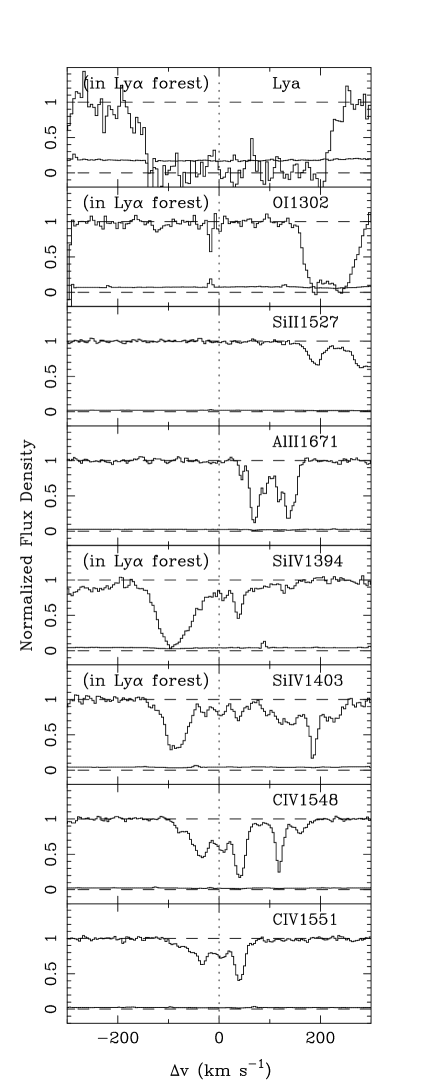
Figure 13: (Sample) Velocity plots of various lines detected in the class B NAL system at $z_{abs}$ = 2.2316 in HE0130$-$4021.

Quasar emission redshifts were obtained from a variety of sources in the literature and they are based primarily on measurements of the peaks of their strong, broad UV emission lines, namely Ly$\alpha$, Si IV and C IV. It is well known that the redshift determined from these particular lines is systematically different from the redshift of the low-ionization lines (i.e., Mg II and the Balmer lines) and the systemic redshift, as given by the narrow, forbidden lines (see, for example, Corbin 1990; Tytler & Fan 1992; Brotherton et al. 1994; Sulentic et al. 1995; Marziani et al. 1996). Even though redshift differences can reach $\sim 4,000~{}{{{\rm km~{}s}^{-1}}}$, in most cases they are within $\pm 1,000~{}{{{\rm km~{}s}^{-1}}}$. In radio-quiet quasars, there is a systematic tendency for the C IV line to be blueshifted relative to the systemic redshift. Most relevant to this work are the results of Tytler & Fan (1992) who study the redshift discrepancies of the UV lines in quasars of comparable redshifts and luminosities to those of our sample. They find a mean blueshift of the UV lines relative to the systemic redshift of 260 km s^-1 and that 90% of the blueshifts are between 0 and 650 km s^-1 (see their Figure 13).

We also list in Table 1 a measure of the radio-loudness of the quasars in our sample, the ratio of the flux densities at 5 GHz and 4400 Å, i.e., ${\cal R}=f_{\nu}(5\;{\rm GHz})/f_{\nu}(4400\;{\rm\AA})$ (following Kellermann et al. 1989, 1994). We adopt ${\cal R}\geq 23$ as the criterion for radio-loudness (instead of the ${\cal R}\geq 10$ adopted by Kellermann et al.) in order to separate cleanly the low-luminosity radio sources in our sample from the high-luminosity ones, which have ${\cal R}>252$. We derived $f_{\nu}(4400\;{\rm\AA})$ from the $V$ or $R$ magnitude using the following equations (Schmidt & Green 1983; Oke & Schild 1970),

$$m_{V}= -2.5\log f_{\nu}(5500{\rm\;\AA})-48.60$$ (1)

$$m_{R}= -2.5\log f_{\nu}(6600{\rm\;\AA})-48.82$$ (2)

and assuming an optical spectral index of $\alpha_{o}=0.44$ (where $f_{\nu}\propto\nu^{-\alpha}$; see Vanden Berk et al. 2001). For Q0241$-$0146 ($z_{em}$ = 4.040) and Q1055$+$4611 ($z_{em}$ = 4.118), the observed optical fluxes obtained from the $V$ magnitude are underestimated because of contamination by the Ly$\alpha$ forest at $z_{abs}$$\sim$ 3.5. Therefore, we boosted these fluxes by dividing by the normalized transmission in the Ly$\alpha$ forest at redshift $z$,

$$T=\exp\left[-0.0037\;(1+z)^{3.46}\right]$$ (3)

(Press, Rybicki, & Schneider 1993). The value of $f_{\nu}(5\;{\rm GHz})$ was obtained from measurements of the flux density at various radio frequencies, assuming a radio spectral index of $\alpha_{r}=0.7$. Thus, our 37 quasars are separated into 12 radio-loud quasars and 25 radio-quiet quasars. Unfortunately, the number of radio-loud quasars that cover the necessary wavelength regions for our analysis is too small to allow a useful statistical study of differences in NAL properties between subclasses.

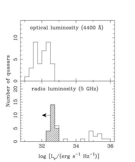
Figure 1: Distributions of optical (4400 Å) and radio (5 GHz) luminosities of the 37 quasars in our sample. The shaded bins in the lower panel correspond to upper limits to the radio flux, as listed in Table 1. Radio-loud objects cluster at 5GHz luminosities between $10^{35}$ and $10^{36}$ ergs s^-1 Hz^-1.

The properties of the quasars in our sample are summarized in Table 1 and Figure 1. Columns (1) and (2) of Table 1 give the quasar name and emission redshift, and columns (3) and (4) the $V$ and $R$ magnitudes. The optical flux density at 4400 Å in the rest frame is given in column (5). Column (6) lists the observed radio flux at the frequency of column (7), if a radio source was detected within 10^′′ of the optical source (e.g., Kellermann 1989). The derived radio flux at 5 GHz is listed in column (8). Column (9) gives the radio-loudness parameter, ${\cal R}$, based on which the quasars are labeled as L (radio-loud) or Q (radio-quiet) in column (10). The distributions of optical (at 4400 Å) and radio (at 5 GHz) luminosities are plotted in Figure 1.

3 Sample of NAL Systems

To construct our sample of NAL systems for statistical analysis, we first examine the 37 quasar spectra, and mark all absorption features that are detected at a confidence level greater than 5$\sigma$, i.e., $[1-R_{c,obs}]/\sigma(R_{c,obs})\geq 5$ ($R_{c,obs}$ is the observed residual intensity at the center of a line in the normalized spectrum and $\sigma(R_{c,obs})$ is its uncertainty). Next, we identify N V, C IV, and Si IV doublets in the following regions around the corresponding emission line:

N V absorption doublets:

from $-5,000~{}{{{\rm km~{}s}^{-1}}}$ to 0 km s^-1 around the N V emission line in the spectra that include this line. If the spectrum extends redward of the N V emission line, we also search for absorption doublets up to $+10,000~{}{{{\rm km~{}s}^{-1}}}$ to the red of the line. The velocity range is relatively narrow for this transition because of contamination from the Ly$\alpha$ forest, which is rather serious at the redshift of our target quasars.

C IV absorption doublets:

from $-70,000~{}{{{\rm km~{}s}^{-1}}}$ to 0 km s^-1 around the C IV emission line in the spectra that include this line. If the spectrum extends redward of the C IV emission line, we also search for absorption doublets up to $+10,000~{}{{{\rm km~{}s}^{-1}}}$ to the red of the line.

Si IV absorption doublets:

from $-40,000~{}{{{\rm km~{}s}^{-1}}}$ to 0 km s^-1 around the Si IV emission line in the spectra that include this line. If the spectrum extends redward of the Si IV emission line, we also search for absorption doublets up to $+10,000~{}{{{\rm km~{}s}^{-1}}}$ to the red of the line.

In Table 1, we list the red limit of the velocity window that we searched for each quasar.

Absorption troughs that are separated by non-absorbed regions are considered to be separate lines, even if they are very close to each other. The equivalent width is measured for each separate line by integrating across the absorption profile. In the case of doublets, we represent the equivalent width by that of the stronger (blueward) member. In total, 261 C IV, 13 N V, and 92 Si IV doublets are identified in this manner. To facilitate detailed studies of the systems, we also searched for single metal lines at the same redshifts as the doublet lines even if these were in the Ly$\alpha$ forest. For the statistical analysis, we construct a complete sample that contains only doublet lines whose stronger members would be detected even in our most noisy quasar spectrum. We convert the absorption-feature detection criterion given above, $[1-R_{c,obs}]/\sigma(R_{c,obs})\geq 5$, to an equivalent width limit using equation (1) of Misawa et al. (2003) and we select absorption features above a certain rest-frame equivalent width. The rest-frame equivalent width limits are set by the spectrum of the quasar Q1330$+$0108 as follows: $W_{min}\;$(C IV)$\;=0.056$ Å at $\lambda\approx 5800$ Å, $W_{min}\;$(N V)$\;=0.038$ Å at $\lambda\approx 5700$ Å, and $W_{min}\;$(Si IV)$\;=0.054$ Å at $\lambda\approx 5800$ Å. These limits apply to the stronger member of each doublet. The “homogeneous” NAL sample defined by these limits contains 138 C IV, 12 N V, and 56 Si IV doublets.

In order to evaluate the column densities ($N$ in cm^-2) and Doppler parameters ($b$ in km s^-1) of NALs, we need to deblend the absorption profiles into narrower components. Thus, we used the software package minfit (Churchill & Vogt 2001) to fit absorption lines with Voigt profiles. In the fitting process, we consider the coverage fraction (defined and discussed in detail in §3.1, below) as a free parameter, as well as the redshift, column density, and Doppler parameter, and we convolve the model with the instrumental profile before comparing with the data. Kinematic components are dropped if a model with fewer components provides an equally acceptable fit to the data. With this procedure, the NALs of the homogeneous sample are deblended into 483 C IV, 41 N V, and 182 Si IV components. The observed profiles of C IV, N V, and Si IV NALs, best-fitting models, and 1$\sigma$ error spectra, are shown on a velocity scale relative to the flux weighted line center in the figures of the Appendix. Almost all the NALs are deblended into multiple components.

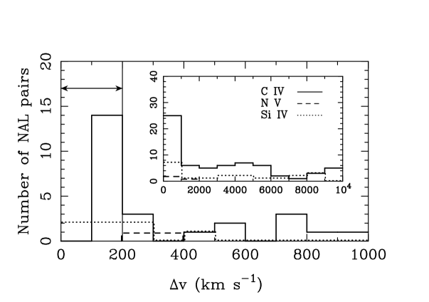
Figure 2: Two point correlation functions for C IV (solid line), N V (dashed line), and Si IV (dotted line) NALs in velocity offset space. Strong clustering is seen at $\Delta v$ $\leq$200 km s^-1 (indicated by arrows in the main panel), especially for C IV NALs. Although we count only the number of pairs which are just next to each other, we get a similar result if we count all combinations.

To refine our sample for statistical analysis, we combine NALs that lie within 200 km s^-1 of each other into a single system (a so-called “Poisson system”). This method is based on the assumption that clustered lines are not physically independent (e.g., Sargent, Boksenberg, & Steidel 1988). We chose this clustering velocity after constructing the distribution of velocity separations between C IV NALs, which we show in Figure 2. We note that our adopted clustering velocity differs from the value of 1,000 km s^-1 adopted in previous papers (e.g., Sargent et al. 1988; Steidel. 1990; Misawa et al. 2002). We obtain 150 Poisson systems in this manner, of which 124, 12, and 50 systems contain C IV, N V, and Si IV NALs, respectively. All NALs are also classified as AALs and non-AALs. We found 18 associated Poisson systems, of which 9, 12, and 4 systems contain C IV, N V, and Si IV NALs, respectively.

Hereafter, we will use the terms “(Poisson) system” for a group of NALs within 200 km s^-1 each other, “line” or “doublet” for an individual NAL (that may lie within a Poisson system), and “component” for a narrow kinematic component described by a single Voigt profile (as deblended by minfit). In Table 2 we list the total numbers of systems, lines, and components that we have found for each of the three strong absorption lines of interest, namely C IV, Si IV, and N V.

We compute the flux-weighted center of a line (or a Poisson system) as the first moment of the line profile, i.e.,

$$\lambda_{obs}=\langle\lambda\rangle=\frac{\sum\lambda_{i}\left[1-R(\lambda_{i})\right]}{\sum\left[1-R(\lambda_{i})\right]}\;,$$ (4)

and the line dispersion, $s$, via

$$s_{\lambda}=\sqrt{\langle\lambda^{2}\rangle-\langle\lambda\rangle^{2}}\;,$$ (5)

where $\langle\lambda^{2}\rangle$ is the second moment of the line profile, given by

$$\langle\lambda^{2}\rangle=\frac{\sum\lambda_{i}^{2}\left[1-R(\lambda_{i})\right]}{\sum\left[1-R(\lambda_{i})\right]}\;,$$ (6)

The above sums are evaluated over the entire width (full width at zero depth) of a line. The quantity $R(\lambda_{i})$ is the intensity at pixel $i$ in the normalized spectrum and $\lambda_{i}$ is the wavelength of that pixel. Using the above quantities, we obtain the flux-weighted line width from

$$\sigma(v)=\sqrt{2}\;s_{v}=\sqrt{2}\left(\frac{s_{\lambda}}{\langle\lambda\rangle}\right)\;c\hskip 14.22636pt{\rm(km}\ {\rm s}^{-1}{\rm)},$$ (7)

Using the flux-weighted wavelength of a line we compute its flux-weighted redshift, and then its velocity offset by the relativistic Doppler formula, i.e.,

$$\beta\equiv\frac{{{v_{shift}}}}{c}=-\frac{(1+z_{em})^{2}-(1+z_{abs})^{2}}{(1+z_{em})^{2}+(1+z_{abs})^{2}}\;,$$ (8)

where $z_{em}$ and $z_{abs}$ are the emission redshift of the quasar and the absorption redshift of the line, respectively. The wavelengths, redshifts, velocity offsets, and flux-weighted widths of detected lines, computed as described above, are given in the Appendix, where we also include NALs that do not meet the rest-frame equivalent width criterion for our homogeneous sample (i.e., they have $W_{rest}<W_{min}$).

3.1 Partial Coverage Analysis

We identified intrinsic NAL candidates by looking for absorption troughs that were diluted by unocculted light from the background source. The optical depth ratio of doublet lines, such as C IV, Si IV, or, N V, sometimes deviates from the value of 2:1 expected from atomic physics. This discrepancy can be explained if the absorber covers the background flux source only partially, and the unabsorbed flux changes the relative depth of the lines (e.g., Wampler et al. 1995; Barlow & Sargent 1997; Hamann et al. 1997a; G99). However, there are other possible explanations, such as local emission by the absorbers (Wampler, Chugai, & Petitjean 1995) and scattering of background photons into our line of sight (G99). We assume the simplest model, in which the absorber has a constant optical depth across the projected area (i.e., a homogeneous model). Then, the observed intensity as a function of velocity from the line center in the normalized spectrum is given by

$$R(v)=\left[1-C_{f}(v)+C_{f}(v)\;e^{-\tau(v)}\right]\;,$$ (9)

where $C_{f}(v)$ is the fraction of background light occulted by the absorber (hereafter, the “coverage fraction”), and $\tau(v)$ is the optical depth at velocity $v$. If a NAL system consists of many kinematic components (the most common case), these are combined by multiplying the individual Voigt profiles after making the appropriate adjustments for partial coverage, following equation (9). Thus we describe the final normalized residual intensity by the product

$$R(v)=\prod_{k}\left[1-C_{f,k}(v)+C_{f,k}(v)\;e^{-\tau_{k}(v)}\right],$$ (10)

where the index $k$ labels different kinematic components. This assumption is quite safe if the components do not overlap significantly in velocity, and is still a good approximation if one component dominates at each wavelength.

If we measure the optical depth ratio of doublet lines with oscillator strength values of 2:1 (e.g., C IV, N V, and Si IV) by fitting their profiles, we can evaluate the coverage fraction as a function of velocity across the line profile as

$$C_{f}(v)=\frac{\left[1-R_{r}(v)\right]^{2}}{1+R_{b}(v)-2R_{r}(v)},$$ (11)

where $R_{r}$ and $R_{b}$ are the continuum normalized intensities of the weaker (redder) and stronger (bluer) members of the doublet (see, for example, Barlow & Sargent 1997). G99 refined this technique by considering two background sources: the continuum source and the broad emission line region (hereafter BELR). In this composite picture the total coverage fraction can be expressed as a weighted average of the coverage fractions of the two regions, namely,

$$C_{f}(v)=\frac{C_{c}(v)+w(v)\;C_{BELR}(v)}{1+w(v)},$$ (12)

where $C_{c}(v)$ and $C_{BELR}(v)$ are the coverage fractions of the continuum source and the broad emission line region, and $w(v)$ is the ratio of the broad line flux to the continuum flux at a given pixel in the absorption-line profile.

It is quite possible for the absorber to have different optical depths along different paths (i.e., an inhomogeneous model; deKool, Korista, & Arav 2002). Nonetheless, by exploring this inhomogeneous model, Sabra & Hamann (2005) found that the average optical depths derived from homogeneous and inhomogeneous models are consistent with each other within a factor of $\leq$1.5, unless a small fraction of the projected area of the absorber has a very large optical depth. Moreover, in most cases, one can find acceptable fits to the absorption profile using a simple combination of just a few Voigt components. Therefore, we adopt the homogeneous optical depth model, as described by equation (11), with the understanding that $C_{f}$ describes the fraction of all background photons that pass through the absorber. We consider the composite picture described by equation (12), only if it critically affects our conclusions.

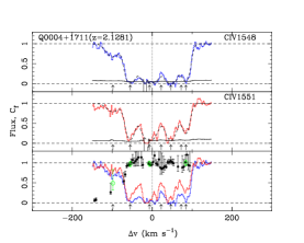
Figure 12: (Sample) Results of partial coverage analysis applied to 206 C IV, N V, and Si IV doublets. Velocities are defined relative to the flux-weighted center of the system, as given in the first line of each block of Table 5. The first two panels of each set show the profiles of the blue and red members of a doublet on a common velocity scale, with the model profile produced by minfit superposed as a dashed line. The positions of the kinematic components making up the model are marked with upward arrows in the bottom of each panel. The third panel of each set shows the two profiles together, along with the resulting coverage fractions and their 1$\sigma$ error bars. The coverage fraction determined by the pixel-by-pixel method is plotted in the form of black filled circles, while the coverage fraction determined by the fitting method is plotted in the form of green open circles.

We use two methods to evaluate $C_{f}$; (i) the pixel-by-pixel method (e.g., G99), in which we apply equation (11) to each pixel in the normalized spectrum, and (ii) the fitting method (e.g., Ganguly et al. 2003) in which we fit the absorption profiles using minfit, treating $C_{f}$ as well as $\log N$, $b$, and $z_{abs}$ as a free parameter. In the former case we obtain a value of $C_{f}$ for each pixel in the line profile, while in the latter case we obtain a value of $C_{f}$ for each kinematic (Voigt) component. Our derived $C_{f}$ values are subject to a number of additional uncertainties resulting from line blending, uncertainties in the continuum fit, the convolution of the spectrum with the line spread function (LSF) of the spectrograph (G99; only applies to the pixel-by-pixel method), and Poisson errors in regions with weak lines (only applies to the fitting method). The methodology for assessing these uncertainties was developed in M05 with the help of extensive simulations. We do not use spectral regions that are strongly affected by these uncertainties, and we consider these sources of error when evaluating whether $C_{f}$ deviates from unity, as described below. The $C_{f}$ values evaluated by both of the above methods are overplotted on the observed spectrum of each doublet shown in Figure 12 of the Appendix.

The minfit routine sometimes gives unphysical coverage fractions such as ${{C_{f}}}<0$ or ${{C_{f}}}>1$. Tests by M05 showed that coverage fractions produced by minfit are very sensitive to continuum level errors, especially for very weak components whose $C_{f}$ values are close to 1, which suggests a cause for these unphysical results. In such cases, other fit parameters, such as the column density and Doppler parameter, have no physical meaning. Therefore we re-evaluate them assuming ${{C_{f}}}=1$ (with no error bar) for those components, and by refitting the rest of the line.

Based on the results of the coverage fraction analysis, we separate all NALs into three classes based on the reliability of the conclusion that they are intrinsic: classes A and B respectively contain “reliable” and “possible” partially covered NALs (i.e., intrinsic NAL candidates), and class C consists of NALs with no evidence for partial coverage (i.e., intervening or unclassified NALs). We may regard classes A–C as including progressively smaller fractions of intrinsic NALs and we will treat them as such in our subsequent statistical analysis.

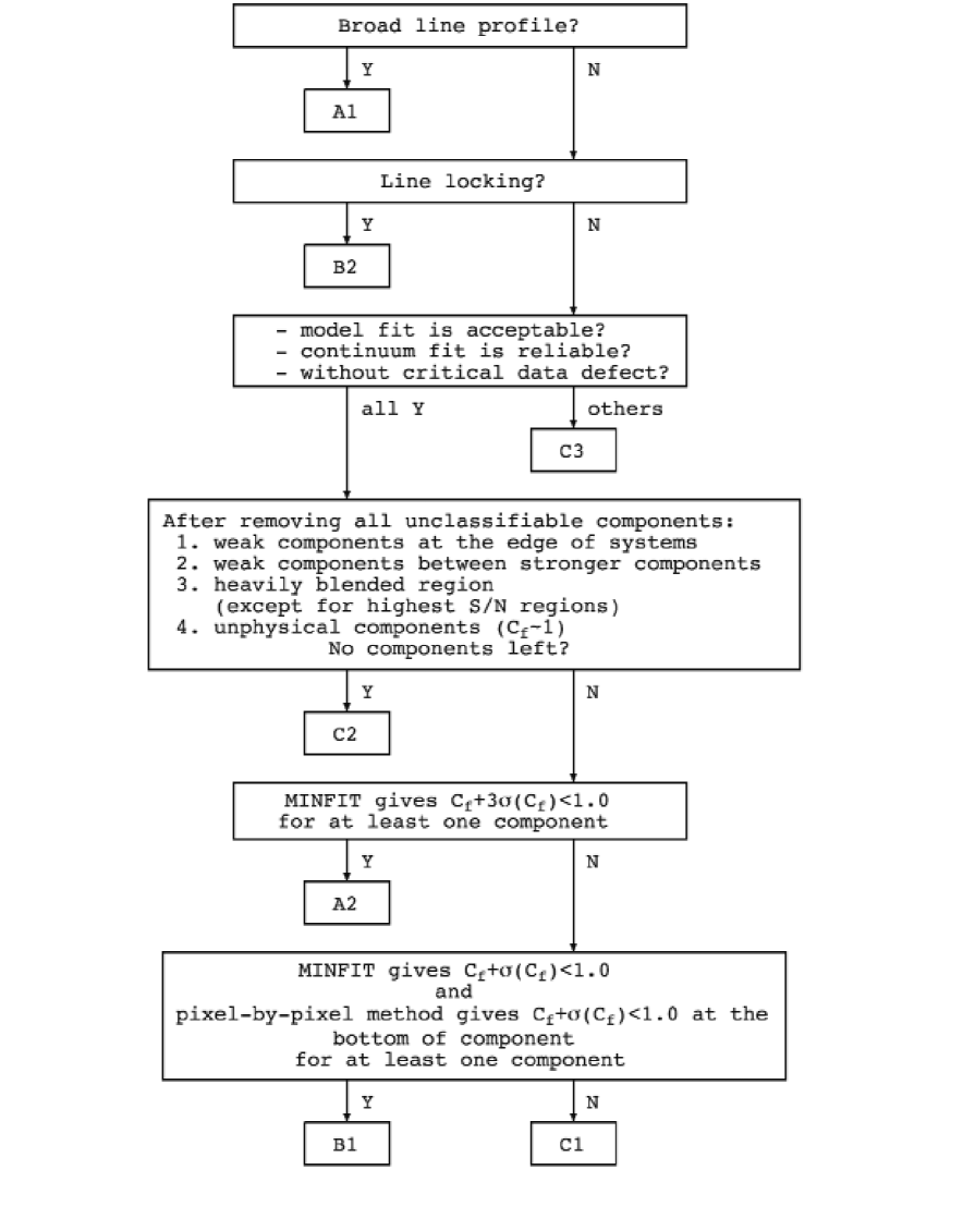
Figure 3: Flow chart illustrating our scheme of NAL classification. The classes indicate how reliably we can determine whether the NALs are intrinsic or not, based on partial coverage analysis. A more detailed discussion of this scheme is given in §3.1 of the text.

We classified four mini-BALs as class A systems. We also classified three NALs into class B, although they did not exhibit partial coverage, because they show line-locking, which is often seen in intrinsic NALs at ${{z_{abs}}}\sim{{z_{em}}}$. In the list below and in the flow chart of Figure 3, we give the criteria and method that we used to classify NALs into reliability classes.

Class A:

Reliable intrinsic NAL candidates:

A1:

smooth and broad (self-blended) line profile (i.e., mini-BAL).

A2:

minfit gives $C_{f}$$+$ 3$\sigma$($C_{f}$) $<$ 1 for at least one component.

Class B:

Possible intrinsic NAL candidates:

B1:

Both minfit and the pixel-by-pixel method give $C_{f}$$+$ $\sigma$($C_{f}$) $<$ 1 at the center of a component for at least one kinematic component.

B2:

line-locked.

Class C:

Lines without partial coverage and unclassifiable lines:

C1:

minfit gives ${{C_{f}}}+\sigma({{C_{f}}})\geq 1$ for all components.

C2:

No components can be used for classification because they suffer from systematic errors as described in the next paragraph.

C3:

The system is not acceptable for classification because of problems due to model fit, continuum fit, or critical data defect.

During line classification, we ignore components that satisfy the following criteria. These were established by following the same procedure to fit strong Mg II doublets identified in the same spectra. For the strong Mg II lines we would expect full coverage for all components, but we find $C_{f}$ to be inconsistent with unity if these criteria apply:

1. Weak components at the edge of a system.

2. Weak components between much stronger components.

3. Components in a heavily blended region (except for regions with extremely high S/N).

4. Components for which we obtained unphysical values of $C_{f}$ in the first fitting trial. As we noted above, we set ${{C_{f}}}=1$ for such components and repeat the fit for the other components in the system.

If at least one component of a NAL satisfies one of the criteria for class A or B, we would classify the NAL as an intrinsic NAL candidate, even if the other components are consistent with full coverage. This applies even for a Poisson system for which only one component in one of the separate lines satisfies the class A or B criteria. Also, if a Poisson system has more than one doublet transition detected and one or more of the transitions (C IV, N V, or Si IV) belongs in class A, it is considered a class A intrinsic system. Similarly, such a system will be considered a class B system if one or more transitions fall in class B (and none is class A).

Placing a Poisson system in class A or B if only one component satisfies the classification criteria involves the following caveat: the class A or B NAL may be superposed on an intervening system by chance. We have thus evaluated the probability of this chance superposition, using the information in Table 3. For example, we have searched for associated C IV NALs in a velocity range $\delta\beta=0.17$ and found 3 class A+B and 6 class C NALs. Since each NAL typically spans a velocity window of 200 km s^-1 or less, the class C NALs cover 2.4% of this velocity window. Therefore, the probability that any one of the 3 class A+B NALs would be blended with a class C NAL (i.e., the expected number of blends) is 0.07. Similarly, we estimate the number of blends to be 0.25 in the non-associated C IV velocity range, 0.03 in the N V velocity range (associated only), and 0.07 in the Si IV velocity range (non-associated only). Thus, we conclude that the danger of a blend is negligible.

In our final sample of 150 Poisson NAL systems, 28 fall into class A, 11 into class B, and 111 into class C. The number of systems, lines, and components are summarized in Table 2. In the Appendix, we list the detailed classification results, along with the subcategory numbers that give the basis for the classification (e.g., A2, C3, …). In the Appendix, we also give detailed comments on individual NAL systems. In Table 2, we give a census of the resulting Poisson systems, NALs and kinematic components.

4 Results

Using the complete NAL sample constructed in the previous section, we first investigate the density of NALs per unit redshift interval and per unit velocity interval (i.e., the velocity offset distribution, $dN/dz$ and $dN/d\beta=c\;dN/dv$, respectively). Next, we examine the relative numbers of intrinsic NALs in different transitions. This is of interest because these relative numbers could be indicative of the ionization structure of the absorbers and also of their locations relative to the continuum source. Our analysis provides only lower limits on the intrinsic NAL fractions, because intrinsic absorber need not always to show partial coverage, and because some of our sample quasar spectra cover only very small redshift windows for NAL detection. We also examine the distributions of coverage fractions and line profile widths, and consider the ionization conditions of the intrinsic NALs in our sample. Finally, we briefly compare the properties of quasars and the properties of intrinsic NALs.

4.1 Velocity Offset and Equivalent Width Distribution

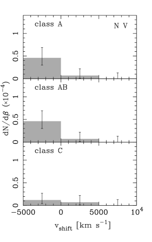
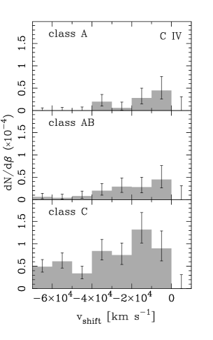
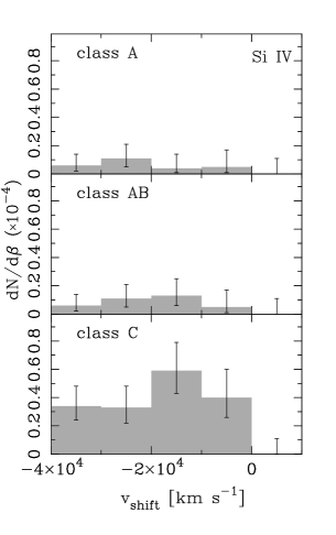
Figure 4: Velocity offset distribution of C IV, N V, and Si IV systems. For each transition we plot separately the distribution of class A systems (reliable), class A+B systems (reliable+possible), and class C systems (intervening/unclassified).

In evaluating $dN/dz$, we exclude segments of spectra in echelle order gaps, which affect about 8.8%, 16.0%, and 23.0% of the spectral regions at $\sim$5,500 Å, $\sim$6,000 Å, and $\sim$6,500 Å, respectively. We implicitly assume that all NALs arise in outflows from the quasars and we use the velocity offset computed by equation (8). In Table 3, we summarize our derived values of $dN/dz$ and $dN/d\beta$ for different transitions and for different velocity offsets relative to the quasar, and we also break down the results by reliability class. The velocity offset distributions of C IV, N V, and Si IV NALs are presented in Figure 4, broken down according to reliability class. It is noteworthy that intrinsic NAL candidates (i.e., class A and B) are found not only among AALs but also among non-AAL systems.

In previous studies using low resolution spectra, the velocity offset distributions of C IV NALs are found to be almost uniform up to ${{v_{shift}}}\sim-70,000~{}{{{\rm km~{}s}^{-1}}}$ (the maximum velocity at which the C IV doublet can be detected without blending with the Ly$\alpha$ forest). However, a significant excess of AALs was found within 5,000 km s^-1 of radio-loud and steep-spectrum quasars (Young, Sargent, & Boksenberg 1982; Richards et al. 1999, 2001; F86). Weymann et al. (1979) presented evidence that the distribution of intrinsic C IV NALs extends up to ${{v_{shift}}}\sim-18,000$ km s^-1. Richards et al. (1999) found an excess of C IV NALs with ${{v_{shift}}}\lower 3.00003pt\hbox{$\,\buildrel>\over{\sim}\,$}-65,000~{}{{{\rm km~{}s}^{-1}}}$ in optically luminous quasars, in radio-quiet over radio-loud quasars, and in flat-radio spectrum quasars over steep-radio spectrum quasars. Our results show no remarkable excess of NALs in radio-loud quasars, nor any strong excess of NALs near the quasars in either the radio-loud or quiet subsamples. This is not surprising, however, since our subsamples of radio-loud and radio-quiet quasars are relatively small and heterogeneous.

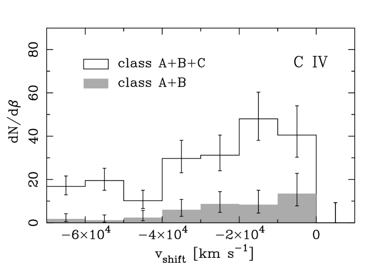
Figure 5: Velocity offset distribution of all C IV systems compared to the distribution of class A+B (reliably and possibly intrinsic) C IV systems.

Considering all C IV NALs (from classes A, B, and C) together, we do find (see Table 3) that, for C IV NALs the values of $dN/dz$ and $dN/d\beta$ in associated regions are about twice as large as those in non-associated regions, in general agreement with the results of Weymann et al (1979). In Figure 5, we show the velocity offset distribution of all C IV NALs from our survey compared to that of class A$+$B NALs.

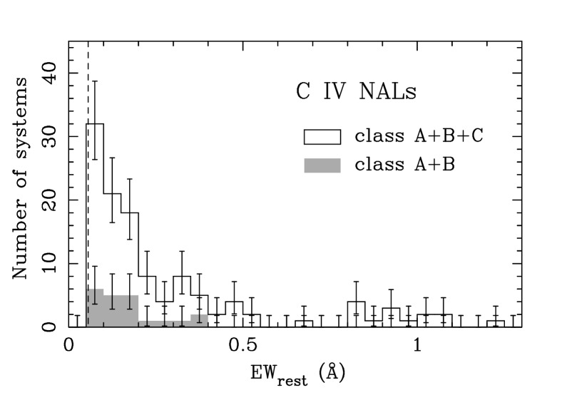
Figure 6: Distribution of rest-frame equivalent width of all C IV systems, compared to the distribution of class A+B (reliably and possibly intrinsic) C IV NALs. The vertical dashed line marks our detection limit of 0.056 Å.

The distribution of rest-frame equivalent widths of the C IV Poisson systems detected in our survey is shown in Figure 6. This distribution rises sharply towards our detection limit of 0.056 Å. We note that the vast majority of our NALs are considerably weaker than those included in previous surveys at low spectral resolution. For example, the survey of Weymann et al. (1979) has a rest frame equivalent width limit of about 0.6 Å (higher than 87% of the NALs in our C IV sample) while the surveys of Young et al. (1982) and F86 have a detection limit of 0.3 Å (higher than 70% of the NALs in our sample). The more recent Vestergaard (2003) study was also conducted using low spectral resolution, so it focused on C IV absorption lines stronger than $\sim$0.3 Å.

A comparison of the equivalent width distributions between our study and these previous low resolution studies is a useful indication of possible biases due to quasar properties. However, such a comparison must focus only on our stronger systems. Also, we must group together different lines that fall within 200 km s^-1 of each other in order to compare with systems found at low resolution (as we did in Figure 6). First we focus on systems with $W_{r}$(C IV) $>$ 1.5 Å since we are concerned about possible biases due to rejecting BAL quasars from our sample, and since Vestergaard (2003) targeted the strongest systems as likely intrinsic candidates. If we take into account Vestergaard’s different method of measuring the equivalent width of C IV, we find that her sample includes 6/114 quasars that have systems with $W_{r}$(C IV) $>$ 1.5 Å. However, the Vestergaard (2003) sample has approximately equal numbers of radio-loud and radio-quiet quasars, unlike ours, in which only 1/3 of the quasars are radio-loud. If we consider only her radio-quiet sample, only 1/48 quasars has a C IV NAL with $W_{r}$(C IV) $>$ 1.5 Å. In her radio-loud sample, 5/66 quasars have very strong C IV NALs. Thus we would predict that in our sample of $37$ quasars (with only $12$ radio-loud) we would find $1.4$ very strong C IV NALs. Though we did not find any, our number is certainly consistent with this estimate, and we do find a system with $W_{r}$(C IV) $\sim$1.0 Å, just below that limit. We note that due to the nature of Vestergaard’s study, her sample has a larger than representative fraction of radio-loud quasars. Our sample also has a somewhat larger fraction of radio-loud quasars (37%) compared to the general population ($\sim$10%), which would lead to a bias towards detecting very strong NALs compared to the general population.

We next consider somewhat weaker NALs, down to $W_{r}$(C IV) = 0.3 Å, to facilitate another comparison with the work of Vestergaard (2003). She found that 27% of the quasars in her sample had C IV absorption for which the sum of the equivalent widths of the two members of the doublet were $>0.5$ Å. In our sample, we only have 13 quasars for which the most of the C IV associated region is covered. Of those 13 quasars, 9 have $W_{r}$(C IV) $>$ 0.056 Å NALs, but only 1(8%) has $W_{r}$(C IV) $>$ 0.3 Å. This is somewhat smaller than we would predict (3.5/13 = 27%) based on Vestergaard’s results, however we again note the differences in the radio properties between the samples. Furthermore, we do not have full coverage of the associated region in all of the 13 quasars, and only 3 of the 13 are radio-loud. It is also worth noting that typically the Vestergaard (2003) quasars are 1-2 magnitudes less luminous than the quasars in our sample.

4.2 Line Width Distribution

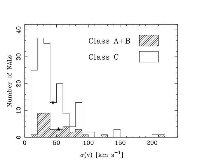
Figure 7: Distribution of the flux-weighted line width ($\sigma(v)$; calculated by eqn. 4) of intrinsic NALs (class A and B) and intervening/unclassified NALs (class C). The filled stars indicate the average $\sigma(v)$-values for intrinsic NALs (53.4 km s^-1) and intervening NALs (44.5 km s^-1).

Historically, it has been very difficult to separate intrinsic NALs from intervening NALs without high resolution spectra because of the similarities of their line profiles. However, if intrinsic NALs arise from absorbers similar to those producing BAL and mini-BAL systems (widths$\,\buildrel>\over{\sim}\,$2,000 km s^-1), they could have larger widths compared to those of intervening NALs. If a tendency for large widths is found among intrinsic NALs, this may be used as an additional indicator of their nature. In Figure 7, we compare the distribution of the flux-weighted line width [$\sigma(v)$; see eqn. (7)] of intrinsic NALs (classes A and B) to that of intervening/unclassified NALs (class C). We do not see any substantial differences between the distributions that would allow us to distinguish between intervening and intrinsic NALs. The average value of $\sigma(v)$ for intrinsic NALs (53.4 km s^-1) is slightly larger than that for intervening NALs (44.5 km s^-1). A Kolmogorov-Smirnov test gives a probability of 12% that the two distributions have been drawn by chance from the same parent population.

4.3 Relative Numbers of Intrinsic NALs in Different Transitions

The numbers of C IV, N V, and Si IV NALs in each of the coverage fraction classes are listed in Table 3. We also list in Table 3 the values of $dN/dz$ and $dN/d\beta$ for each type of system. Based on these values, reliable (class A) intrinsic NALs make up 11% of all C IV NALs, 75% of all N V NALs, and 14% of all Si IV NALs. These fractions increase to 19%, 75%, and 18% after adding possible intrinsic NALs (class B). Concentrating on different transitions in turn, we note the following:

N V. —

The above fractions of N V NALs that are intrinsic refer only to the AAL velocity range (${{v_{shift}}}\leq-5,000~{}{{{\rm km~{}s}^{-1}}}$) because contamination by the Ly$\alpha$ forest prevented us from searching for NALs at larger velocity offsets. Nonetheless, it is worth noting that 3/4 of these associated N V NALs are intrinsic. The density of intrinsic NALs in the associated region is thus quite high ($dN/dz=3.4$ and $dN/d\beta=13.7$).

C IV. —

The fraction of intrinsic C IV NALs in associated regions (33%) is slightly higher than the fraction we found in non-associated regions (10%–17%). If the fraction of intrinsic NALs at ${{v_{shift}}}>-5,000~{}{{{\rm km~{}s}^{-1}}}$ was actually the same as the fraction at ${{v_{shift}}}<-5,000~{}{{{\rm km~{}s}^{-1}}}$, the probability that 3 or more out of 9 C IV AALs are intrinsic to the quasar (based on the binomial distribution) is 5.1% . If we consider only the radio-quiet subsample, the probability is even smaller, 1.2%. In the radio-loud sample, we found no intrinsic C IV AALs, but this does not mean that there is an actual deficiency of intrinsic C IV AALs, because our 12 spectra of radio-loud quasars have only a small redshift path for detecting C IV AALs ($\delta z=0.64$).

Si IV. —

We found no intrinsic Si IV AALs in the redshift window of $\delta z=1.26$ that we searched.

4.4 Fraction of Quasars Showing Intrinsic NALs

To investigate the geometry of absorbing gas around the quasars we count the number of intrinsic NALs per quasar, and we evaluate the fraction of quasars hosting intrinsic NALs. These values constrain the global covering factor ($\Omega/4\pi$) of the continuum source and BELR by the absorber and the distribution of absorbing gas around the quasar central engine. At $z<1$, G01 found that radio-loud, flat-spectrum quasars with compact radio morphologies (i.e., with a face-on accretion disk) lack AALs down to a limiting equivalent width of $W_{rest}=0.34$ Å. This suggests that the presence of intrinsic NALs depends on the inclination of the line of sight to the symmetry axis of the quasar central engine.

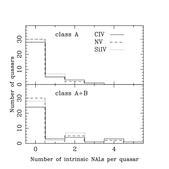
Figure 8: Distribution of the number of intrinsic systems per quasar. The top panel includes only class A (reliable) systems, while the lower panel includes class A+B (reliable+possible) systems. In each panel we show the distribution of C IV systems as a solid line, the distribution of N V systems as a dashed line and the distribution of Si IV systems as a dotted line. We note that the number of intrinsic systems per quasars in these histogram is strictly a lower limit (see discussion in §4 of the text).

In Table 3 we list the fraction of NALs that are intrinsic and the fraction of quasars that have intrinsic NALs. We count only quasars that have velocity windows for NAL detection of $\delta\beta>0.01$ ($\delta v>3,000~{}{{{\rm km~{}s}^{-1}}}$) in the transition of interest. In Figure 8, we plot the distribution of the number of intrinsic NALs per quasar. The upper panel shows the distribution of only class A NALs, while the lower panel includes both class A and B NALs.

About 24% of quasars (9 out of 37) have at least one reliable (class A) intrinsic C IV NAL. Taking possible (class B) NALs into consideration, 32% (12 out of 37) of quasars have at least one intrinsic C IV NAL. The corresponding fractions for N V and Si IV (19–24%) are lower than for C IV. However, we cannot immediately conclude that the global covering factor of C IV absorbers is higher than those of N V and Si IV, because all of these values are just lower limits since some intrinsic NALs could have full coverage and also because we were not able to search for N V NALs over a wide range in $v_{shift}$. If we consider all three transitions, 43% (16 out of 37) of the quasars have at least one class A intrinsic NAL (in at least one of the three transitions) and 54% (20 out of 37) of the quasars have at least one class A or class B intrinsic NAL.

4.5 Distribution of Coverage Fractions

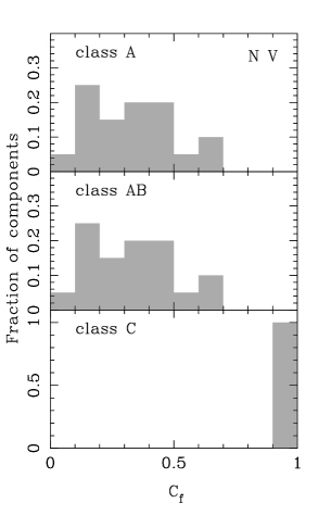
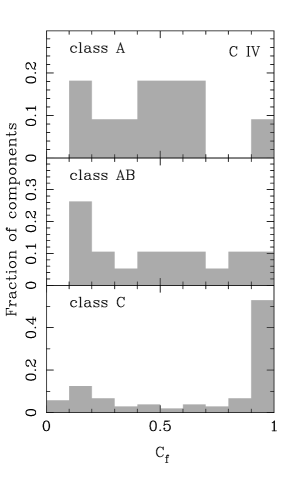
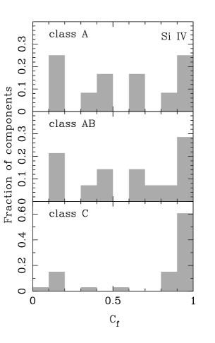
Figure 9: Distribution of coverage fractions of C IV, N V, and Si IV NAL components. We plot only components whose $C_{f}$ values are physical (i.e., $0<{{C_{f}}}$ and ${{C_{f}}}<1$) and evaluated with high reliability (i.e., $\sigma$($C_{f}$) ¡ 0.1). For each transition we plot separately the distribution of class A NALs (reliable), class A+B NALs (reliable+possible), and class C NALs (intervening/unclassified). Even though some class-C NALs have ${{C_{f}}}<1$. These values are consistent with 1 within their $1\sigma$ errors.

The normalized distribution of the coverage fraction for individual NAL components is presented in Figure 9, where it is broken down by transition and by reliability class. We plot only components for which we get physical covering fractions. The mean and median values of $C_{f}$ in class A$+$B NALs are, respectively, 0.38 and 0.33 for N V, 0.50 and 0.48 for C IV, and 0.56 and 0.52 for Si IV. Putting together NALs from all three transitions, we find mean and median values of $C_{f}$ of 0.48 and 0.45, respectively. Focusing on the $C_{f}$ distribution among C IV NALs (the largest of all populations shown in Fig. 9) we note that in class A$+$B NALs are distributed uniformly between 0 and 1, while more than half of the class C NALs have coverage fraction larger than 0.9 (this was one of the criteria for placing a component in this class).

In addition to the NAL components shown in Figure 9, Table 2 shows that 56%, 34%, and 58% of C IV, N V, and Si IV NAL components in the homogeneous sample have unphysical measured $C_{f}$ values. This usually indicates a doublet ratio slightly greater than two. If we assume that all components whose $C_{f}$ values are unphysical or are consistent with full coverage (i.e., ${{C_{f}}}+\sigma({{C_{f}}})\geq 1.0$) really have full coverage, we find that 73% (355/483), 41% (17/41), and 72% (131/182) of C IV, N V, and Si IV components cover the background flux sources. If we consider only intrinsic systems, these fractions would be 59% (44/75)), 26% (8/31), and 31% (8/26), respectively. Generally, we display only components whose $C_{f}$ values are physical and whose errors are small enough (i.e., $\sigma$($C_{f}$) $<$ 0.1) to avoid any uncertainties from $C_{f}$ value estimation.

For some intrinsic NAL systems, coverage fractions have been determined for more than one transition (e.g., Ganguly et al. 2003; Yuan et al. 2002). G99 found that the C IV, N V, and Si IV coverage fractions are similar to each other for a few systems, while Petitjean & Srianand (1999) and Srianand & Petitjean (2000) noted that higher ionization transitions tend to have larger coverage fraction than lower ionization transitions. This type of effect could occur if the sizes of the background sources (i.e., continuum source, BELR) and/or the absorber are not the same for all transitions.

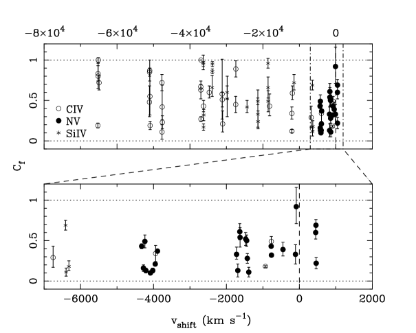
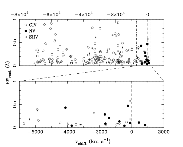
Figure 10: Relationship between the velocity offset of intrinsic NALs (class A+B) from the quasars and their coverage fraction (top) and rest-frame equivalent width (bottom). In the top figure, we plot only components whose $C_{f}$ values are physical (i.e., $0<{{C_{f}}}$ and ${{C_{f}}}<1$) and evaluated with high reliability (i.e., $\sigma$($C_{f}$) $<$ 1.0). The upper panel in each case presents a wide velocity region (from $-80,000$ to 10,000 km s^-1). The lower panel focuses on the narrower velocity window from $-7,000$ to 2,000 km s^-1. Open circles denote C IV NALs, filled circles denote N V NALs, and asterisks denote Si IV NALs.

Unfortunately, our results do not allow a direct comparison between different transitions within the same system because (a) detecting multiple transitions from the same system was rather rare and (b) multiple components in the same intrinsic NAL often have different $C_{f}$ values, preventing us from assigning a single $C_{f}$ value to a NAL or a system. Therefore, we compare the overall distributions of the physically meaningful (between 0 and 1) $C_{f}$ values of the 34 C IV, 25 N V, and 20 Si IV components found in 23 C IV, 9 N V, and 9 Si IV class A and B intrinsic NALs, in Figure 9. An alternative illustration of these distributions is shown in Figure 10 where we plot the coverage fraction of each NAL component against its offset velocity. A visual inspection of these two figures suggests that the associated intrinsic N V NALs prefer smaller values of $C_{f}$ than the C IV and Si IV intrinsic NALs. Nearly all N V components show coverage fractions less than 0.5, while the coverage fractions of C IV and Si IV NALs range from nearly 0 up to nearly 1. This difference is also reflected in the mean and median values of $C_{f}$ reported above. However, a Kolmogorov-Smirnov test yields a probability of 17% that the C IV and N V $C_{f}$ distributions were drawn from the same parent population. Similarly, the probability that the N V and Si IV $C_{f}$ distributions were drawn from the same parent population is 7%. Larger samples are needed to reach a definitive conclusion.

4.6 Other Relations between Intrinsic NAL and Quasar Properties

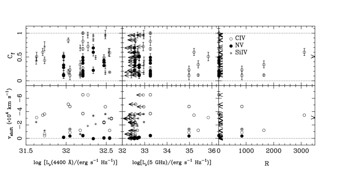
Figure 11: Plots of NAL parameters (i.e., $C_{f}$ and $v_{shift}$) against quasar properties (i.e., $L_{\nu}$(4400 Å), $L_{\nu}$(5 GHz), and ${\cal R}$). Only intrinsic NAL components (class A+B), whose $C_{f}$ values are physical (i.e., $0<{{C_{f}}}$ and ${{C_{f}}}<1$) and evaluated with high reliability (i.e., $\sigma$($C_{f}$) $<$ 0.1), are plotted. For quasars that were not detected in the radio, we plot upper limits on $L_{\nu}$(5 GHz) and ${\cal R}$. Open circles denote C IV NALs, filled circles denote N V NALs, and asterisks denote Si IV NALs.

With our large sample of intrinsic NALs we can search for relations between the NAL properties (e.g., $C_{f}$ $vs$ $v_{shift}$ and rest equivalent width $vs$ $v_{shift}$) and the properties of the quasars hosting them ($L_{opt}$, $L_{radio}$, ${\cal R}$). Figure 11 shows plots of these parameters against each other, including class A$+$B NALs. For some quasars, we plot just the upper limits on $L_{radio}$, since the corresponding radio sources have not been detected. We do not find any significant correlations in these plots. We also searched for a correlation between the offset velocity and the coverage fractions and rest equivalent width of C IV, N V Si IV NALs but we did not find any (see Figure 10)

4.7 Ionization State

Traditionally, BALs have been classified according to their ionization level into HiBALs (high-ionization BALs), LoBALs (low-ionization BALs), and FeLoBALs (extremely low-ionization BALs that show Fe II lines; e.g., Weymann et al. 1991). Motivated by the classification of BALs and by the work of Bergeron et al. (1994) on classifying intervening NALs, we attempt to classify intrinsic NALs (classes A plus B) in a similar manner. We consider the range of conditions in the systems presented in this paper in conjunction with our concurrent study of lower redshift intrinsic NALs in the HST/STIS Echelle archive (Ganguly et al. 2007; in preparation). This low redshift sample adds an important element because the O VI doublet can often be examined, unlike in the spectra of $z=2$–4 quasars of this paper for which the Ly$\alpha$ forest is quite thick.

We find that we can classify the intrinsic NALs in our sample into 2 categories according to the relative absorption strengths in various transitions:

Strong C IV NALs. —

In these systems Ly$\alpha$ is often saturated and black. N V is detected in some of these C IV systems, but it is weaker than C IV.

Strong N V NALs. —

The corresponding Ly$\alpha$ lines have an equivalent width that is less than twice the N V $\lambda$1239 equivalent width. C IV is detected in some of these N V systems, but is typically weaker than N V.

To clarify, in the case of a NAL system which has both C IV and N V transitions, we classify it as a strong C IV system if Ly$\alpha$ in the system is black or if the total equivalent width of Ly$\alpha$ is larger than twice the N V equivalent width. Otherwise, we classify them as a strong N V system, even if C IV is stronger than N V.

One possible explanation for the physical difference between C IV and N V systems is a difference in ionization parameter, however the column density, the metallicity, and/or the metal abundance pattern could also affect these conditions. Photoionization models will be required for the conclusive discussion (Wu et al. 2007; in preparation).

We applied the above criteria to 28 class A and 11 class B NALs, and classified them into 28 strong-C IV systems (17 class A and 11 class B) and 11 strong-N V systems (all of them are class A). The ${{z_{abs}}}=2.7164$ system toward HS1700$+$1055 has an O VI doublet which is much stronger than the N V, C IV, and Ly$\alpha$ lines. Although we classified it as an N V intrinsic NAL, it would likely fall in the additional category of a strong O VI system, if we allowed for that category. Finally, we added a subclassification based on the detection of low-ionization (${\rm IP}<25$ eV) or intermediate-ionization (${\rm IP}=35$–50 eV) absorption lines in the same system. We note that BAL systems sometimes have extremely low-ionization transitions such as Mg II (${\rm IP}=15$ eV; e.g., Hall et al. 2002). The results are summarized in Table 4 where we report the transitions detected in each of the above systems. Notes on individual systems and velocity plots are included in the Appendix.

Table 4 shows that among the 28 C IV intrinsic systems, 15 have low-ionization lines, while 25 have intermediate-ionization lines. Two systems (at ${{z_{abs}}}=2.7699$ in Q1425$+$6039 and at ${{z_{abs}}}=2.3198$ in Q1548$+$0917) are sub-DLA systems, which casts some doubt on their intrinsic classification (see the Appendix for a discussion of these individual cases). Nonetheless, we see that more than half of the intrinsic C IV NALs have related low ionization absorption lines. Among the 11 N V systems, 5 have intermediate ionization absorption, and only 1 has low ionization absorption. This is another noteworthy difference between C IV and N V intrinsic NALs.

In 41% of intrinsic systems (16 out of 39) we detect low-ionization transitions, and 55% of quasars (11 out of 20) that have at least one intrinsic system, have at least one system with low-ionization transitions. This is much higher than the fraction of LoBAL quasars among BAL quasars (17% according to Sprayberry & Foltz 1992, 13% according to Reichard et al. 2003).

Unfortunately, O VI is in the Ly$\alpha$ forest or is not covered in our spectra, making it quite difficult to establish the ionization properties of our systems. However, an additional class of O VI associated NALs (possibly intrinsic) has emerged from our study of lower redshift quasars using the STIS/Echelle archive. These O VI systems are sometimes redward of the emission redshift of the quasar, they have relatively weak Ly$\alpha$ lines compared to O VI, and they do not always have partial coverage (Ganguly et al. 2006; in preparation). A few of our N V intrinsic NALs with non-black Ly$\alpha$ may have very strong O VI absorption, and thus could fall in this third category.

5 Discussion

5.1 Evolution of the Frequency of Intrinsic NALs With Redshift

If we associate intrinsic NALs with quasar outflows, their evolution with redshift traces the evolution of quasar outflows. Moreover, since outflow properties depend on the properties of the accretion flow (at least in disk wind models), the redshift evolution of NALs provides constraints on the evolution of quasar fueling rates.

We begin by considering quasars with strong C IV AALs ($W_{rest}\geq 1.5$ Å), which have a high probability of being intrinsic because of their small velocity offsets from the quasars. At intermediate redshifts ($z=1$–2), F86 found strong C IV AALs in 33% of quasars, while G01 detected such a strong C IV AAL in only 2% of low-redshift quasars ($z<1$), and suggested that this fraction increases with redshift. In our high redshift sample ($z=2$–4), we only detect one rather strong AAL with $W_{rest}\sim 1.0$ Å. This could mean that the frequency of strong AALs peaks at $z\sim 2$, which coincides with the redshift at which the quasar density peaks. There are, however, a number of noteworthy caveats to this apparent evolutionary trend, namely (a) the samples used at different redshifts have different optical and radio luminosity distributions (the G01 sample includes a significant fraction of low-luminosity objects, for example), (b) strong AALs appear to prefer steep-spectrum radio-loud quasars (F86; Anderson et al. 1987) which make up different fractions of the above samples (the F86 sample is predominantly radio-loud), and (c) strong AALs need not always be intrinsic, in particular they could come from galaxies in a cluster surrounding the quasar, which are more often found around radio-loud quasars (e.g., Yee & Green 1987, Ellison, Yee, & Green 1991; Yee & Ellison 1993; Wold et al. 2000).

We now turn our attention to the evolution of the fraction of quasars with intrinsic AALs, including weak ones, down to a rest-frame equivalent width of $\sim 50$ mÅ (using samples constructed on the basis of partial coverage or variability). At $z<1.5$, Wise et al. (2004) found that a minimum of 27% of quasars have intrinsic AALs, while at $z\sim 2$, Narayanan et al. (2004) found that a minimum of 25% of quasars host intrinsic AALs. Similarly, G99 find that at least 50% of $z\sim 2$ quasars have intrinsic AALs, and in this study, we find that a minimum of 23% of quasars at $z=2$–4 have intrinsic AALs. These fractions are consistent with each other, especially considering that some of the samples are rather small (only six quasars in the G99 sample). An important caveat here is that all of these results refer to lower limits since NALs that do not show variability or partial coverage can still be intrinsic. This caveat not withstanding, the fraction of quasars hosting intrinsic AALs does not show significant redshift evolution. A closely related question is the redshift evolution of the fraction of AALs that are intrinsic. At $z<1.5$ this fraction is $>21$% (Wise et al. 2004), at $z\sim 2$ it is $>23$% (Narayanan et al. 2004) or $>60$% (G99), and at $z=2$–4 it is $>27$% (this work). Thus, this quantity does not appear to evolve with redshift either, but this conclusion is also subject to the caveat noted above.

5.2 Properties of Intrinsic Absorbers in Our Sample

5.2.1 Range of Coverage Fractions

In non-associated regions (i.e., $|{{v_{shift}}}|>5,000~{}{{{\rm km~{}s}^{-1}}}$), we found that 10–17% of C IV NALs are intrinsic to the quasars. Richards et al. (1999) and Richards (2001) suggested that this fraction is as large as 36%, based on the excess of absorbers at $>5000~{}{{{\rm km~{}s}^{-1}}}$ in steep spectrum as compared to flat spectrum radio-loud quasars. Our estimate is strictly only a lower limit, because not all intrinsic NALs can be identified using partial coverage. If we take both our result that 10–17% of C IV NALs are intrinsic and the Richards et al. number of 36% at face value and try to reconcile them, we conclude that only 30–50% of intrinsic C IV NALs exhibit detectable partial coverage in our sample. We caution that the two samples were selected in different ways, leading to biases. For example, the sample of Richards et al. (1999) has a larger fraction ($\sim 50$%) of radio-loud quasars than our sample ($32$%). However, since they found that intrinsic NALs prefer radio-quiet quasars, the difference between our estimate of the fraction of quasars hosting intrinsic NALs and theirs would be larger than what it appears, leading to a larger number of fully covered intrinsic NALs.

This conclusion is bolstered by the fact that the distribution of measured coverage fractions of intrinsic C IV NALs spans the range from 0 to nearly 1 (within uncertainties). The covering factors are presumably related to the physical sizes of the absorbing structures, which could span a significant range. In this sense there is nothing special about the size corresponding to a covering factor of 1. If there is a cutoff in size, there is no reason it would occur particularly at this value. Thus we strongly expect that many intrinsic absorbers with unit coverage fraction exist.

5.2.2 Ionization Conditions

The wide range of absorber ionization conditions presented in §4.7 (e.g., “strong N V” vs “strong C IV” absorbers) may be a result of a wide distribution of distances of the gas parcels from the continuum source and/or a wide distribution of their densities. The velocity offset of a system can serve as an indicator of its proximity to the continuum source under the assumption that parcels of gas in an outflowing wind are accelerated outwards from the continuum source. Detailed photoionization modeling of selected systems can help us determine whether there is a relation between their ionization state of NAL systems and their apparent outflow velocity, which will allow us to determine whether there is ionization stratification in the outflow. The same models may also provide constraints on the density of the gas. In fact, photoionization models for the associated absorber in QSO J2233$-$606 (Gabel, Arav & Kim 2006) show that the higher-ionization kinematic components are at lower blueshifted velocities than lower-ionization components. Moreover, preliminary results of photoionization models for three of the quasars in our sample (Wu et al. 2007, in preparation) suggest that absorbers at different velocities in the same quasar can have a wide range of densities. An alternative way of constraining the density is through monitoring observations, which can set limits on the recombination time scale of the absorber, hence constrain the density (see, for example, the discussion in Wise et al. 2004, Narayanan et al. 2004, and M05).

It is also important to ask whether the low ionization transitions in intrinsic C IV NALs are aligned with the high ionization transitions. An inspection of the velocity plots of individual systems in the Appendix shows that the line centers and profiles of low-ionization lines in intrinsic NAL systems are almost always similar to those of high-ionization lines. This leads us to conclude that the low-ionization lines arise in the intrinsic absorbers and not in the ISM of the host galaxy.

5.2.3 Intrinsic NALs at Large Velocity Offsets

Our finding (supported by the independent method of Richards 2001) that a significant fraction of NALs, even at high velocity offsets from the quasar redshift, are intrinsic (10–17% of C IV NALs and 15–20% of Si IV NALs) has implications for cosmology since it affects the estimates of the density of intervening systems per unit redshift ($dN/dz$). For example, at $z=2$–4, $dN/dz$ is estimated to be 3.11 for C IV and 1.36 for Si IV systems with a rest frame equivalent width greater than 0.15Å (Misawa et al. 2002). If these values are reduced by 15–30% after correction for intrinsic systems, this would require some adjustment of models for cosmological evolution of these systems. Furthermore, the contamination of the Ly$\alpha$ forest by very high metallicity intrinsic NALs could seriously bias estimations of the metallicity of the forest.

5.3 Implications for Models of Quasar Outflows

The results of our survey have direct implications for models of quasar outflows, whatever the acceleration mechanism.

1. The minimum fraction of quasars with at least one intrinsic NAL (C IV, N V, or Si IV) is 43–54%. If there is an additional family of intrinsic O VI absorbers, without corresponding C IV or N V lines, the minimum fraction of quasars with intrinsic NALs will increase further. This leads to a constraint on the solid angle subtended by the NAL absorbers to the background source(s). We can interpret this result in the context of a simple (but clearly not unique) picture in which all quasars in our sample are similar to each other and the NAL gas is located at intermediate latitudes above the streamlines of a fast, equatorial outflow (a BAL wind). This geometry is similar to that depicted in Figure 13 of G01, although it needs not apply specifically to an outflow launched from the accretion disk; a pressure-driven outflow launched from a distance of an order of 1 pc from the black hole may have a similar geometry. In this picture, the above observational constraint translates directly into the opening angle of the NAL zone, given the opening angle of the BAL wind. For an opening angle of the BAL wind of approximately 7–12^∘ (10–20% of quasars are BAL quasars; e.g., Hamann, Korista, & Morris 1993) the angular width of the NAL zone turns out to be 25–27^∘. In this picture the polar region, at latitudes above the NAL zone may be filled with highly-ionized gas. This idea is consistent with the finding of Barthel, Tytler & Vestergaard (1997) that strong associated C IV NALs with $W_{rest}$ $>$ 3 Å are most common at angles far from the jet axis in radio-loud QSOs (as high as $45^{\circ}$). Such strong NALs may represent intermediate viewing angles between intrinsic NALs and BALs. Other simple interpretations are also possible: for example, the NAL gas may be distributed isotropically around the central engine, or some quasars may be more likely than others to host such absorbers (e.g., the width of the NAL zone may depend on luminosity, as suggested by Elvis 2000).

2. The density of intrinsic (class A$+$B) C IV NALs per unit velocity interval, $dN/d\beta$, increases from 4.1 at ${{v_{shift}}}<-5,000~{}{{{\rm km~{}s}^{-1}}}$ to 18 at ${{v_{shift}}}>-5,000~{}{{{\rm km~{}s}^{-1}}}$. This is a significant increase with a chance probability of only 5%. These results have a number of implications for outflow models. First, the high-velocity NALs (71% of class A+B NALs at ${{v_{shift}}}<-5,000~{}{{{\rm km~{}s}^{-1}}}$) are unlikely to be associated with pressure-driven outflows because these outflows can only reach velocities of order $10^{3}~{}{{{\rm km~{}s}^{-1}}}$. The distribution of $dN/d\beta$ with $\beta$ does not provide a straightforward constraint on the acceleration mechanism because the models do not predict how individual parcels of NAL gas are distributed. One could take the higher value of $dN/d\beta$ at low velocities as an indication of the existence of a separate population of absorbers, which could perhaps be identified with a pressure driven wind. On the other hand, the velocity of a magnetocentrifugal or line-driven accretion disk wind increases smoothly with radius, which may lead to higher density of NALs per unit velocity at low velocities (assuming that the gas parcels are condensations that form near the base of the wind and are accelerated outwards). Economy of means and Occam’s razor favor the latter explanation since it applies to both high- and low-velocity NALs and invokes a single acceleration mechanism. This issue can be addressed observationally by constraining the distance of the low-velocity (associated) NAL gas from the central engine. This can be done by combining constraints on its ionization parameter (obtained from photionization models) with constraints on its density (obtained from variability studies).

3. The C IV column densities derived from fitting the line profiles, can yield a preliminary estimate of the total hydrogen column densities (H I+H II) in the absorbers. More specifically, we can apply the calculations of Hamann (1997) to estimate an upper limit to the hydrogen column density of absorbers in our sample from our highest measured C IV column density of $\log\;N_{\rm C\;IV}=15.86$ (in the $z_{abs}=2.5597$ NAL in HE0130$-$4021). If we assume an abundance of C IV relative to C of $\log\;[N_{\rm C\;IV}/N_{\rm C}]\approx-0.34$ (this limit corresponds to the optimal ionization parameter that maximizes the C IV abundance; see Figure 2 of Hamann 1997) and a solar abundance of C relative to H, $\log\;({\rm C}/{\rm H})=-3.44$ (Grevese & Anders 1989), we obtain $N_{\rm H}\sim 4\times 10^{19}$ cm^-2. If the C abundance is super-solar (e.g., Hamann 1997), this limit will become smaller, of course. Higher total column densities have also been observed in NALs; for example, Arav et al. (2001a) find $\log N_{\rm H}>20.3$ in QSO J2359$-$1241. Moreover, total column densities in BALs can be an order of magnitude higher (e.g., in PG 0946$+$301; Arav et al. 2001b).

   We emphasize that the column densities estimated above refer only to the gas responsible for the C IV NALs. This gas could well have the form of filaments embedded in a hotter medium, as predicted by many models (see §1 and references therein). If that is the case, then the total column density of the outflow can be considerably larger than what we have estimated above. In fact, X-ray spectroscopy of nearby AGNs does indicate a multi-phase absorber structure in which the column density of the hot medium is higher than that of the cold medium by a factor of 30 or more. (e.g., Netzer et al. 2003, Kaspi et al. 2004, and references therein)

For the specific case of radiatively-accelerated outflows, we can ask whether the observed high velocities of some NALs are attainable in the context of the model. Hamann (1998) derives the following expression for the terminal velocity of a radiatively accelerated wind

$$v_{\infty}=9,300\;r_{0.1}^{-1/2}\left({f_{0.1}L_{46}\over N_{22}}-0.1\;M_{8}\right)^{1/2}{{{\rm km~{}s}^{-1}}}\;,$$ (13)

where $r=0.1\;r_{0.1}$ pc is the distance of the absorber from the continuum source, $L=10^{46}\;L_{46}~{}{{{\rm erg~{}s}^{-1}}}$ is the quasar luminosity, $M_{BH}=10^{8}\;M_{8}\;{\rm M}_{\odot}$ is the black hole mass, and $f=0.1\;f_{0.1}$ is the fraction of continuum photons absorbed or scattered by the gas, and $N_{H}=10^{22}\;N_{22}~{}{\rm cm}^{-2}$ is the column density of the absorbing gas. Noting that $L_{46}/M_{8}\approx 0.77\;(L/L_{Edd})$ (where $L_{Edd}$ is the Eddington luminosity) and that $r_{0.1}/M_{8}\approx 2\;\xi_{4}$ ($\xi_{4}\equiv r/10^{4}\;r_{g}$ and $r_{g}\equiv GM_{BH}/c^{2}$ is the gravitational radius), we may recast equation (13) as

$$v_{\infty}=5,000\;\xi_{4}^{-1/2}\left({f_{0.1}\over N_{22}}\;{L\over L_{Edd}}-0.13\right)^{1/2}{{{\rm km~{}s}^{-1}}}\;.$$ (14)

As Hamann (1998) argues, $f_{0.1}\sim 1$ for BAL quasars. The radiation-pressure dominated part of the accretion disk extends up to $\xi_{4}\approx 0.25$ for parameters scaled as above (see Shakura & Sunyaev 1973). According to most models for accretion disk winds (Murray et al 1995; Proga et al. 2000; Everett 2005), the inner launch radius of the wind corresponds to $\xi_{4}\approx 0.06$–0.25. Moreover, the C IV column densities that we find observationally (see discussion above) indicate total hydrogen column densities in NALs corresponding to $N_{22}\sim 0.01$. Under these conditions, radiation pressure can accelerate the NAL gas to terminal speeds well in excess of $10^{5}~{}{{{\rm km~{}s}^{-1}}}$, and the observed blueshifts of intrinsic NALs can be easily explained.

There is an important caveat to the above estimate. We have assumed that the column density that we have measured from the C IV NAL profiles traces all of the matter that is being accelerated. But, as we note earlier in this section, the NAL gas may be embedded in a hot medium and it may represent only a small fraction of the total gas mass. In such a case, the attainable terminal velocity will decrease accordingly. More specifically, if the NAL gas represents up to 10% of the total column density, then equation (14) can still reproduce the observed NAL velocities. But if the total column density is more than an order of magnitude higher than the C IV NAL column density, then a different acceleration mechanism must be sought.

6 Summary and Conclusions

We have constructed a large, relatively unbiased, equivalent width limited sample of intrinsic narrow absorption line (NAL) systems found in the spectra of $z=2$–4 quasars. This sample comprises 124 C IV, 12 N V, and 50 Si IV doublets, which were separated from intervening NALs on the basis of their partial coverage signature. After assessing the reliability of the determination of the intrinsic nature of these NAL systems, 28 are deemed reliably intrinsic (“class A”), 11 are deemed possibly intrinsic (“class B”) and 111 are deemed intervening (or unreliable intrinsic candidates; “class C”). Using this sample of NAL systems, we study their demographics, the distribution of their physical properties, and any relations between them. We also consider the implications of these results for models of outflowing winds. Our findings and conclusions are as follows:

1. The fraction of intrinsic C IV systems in our sample NALs is 11–19%. This value increases to 33% if only associated systems, within 5,000 km s^-1 of the quasar emission redshift, are considered. This is roughly consistent with previous studies of associated C IV NALs at different redshifts and employing different methods. It is important to note, however, that all of the above fractions are, in fact lower limits to the true fractions. The fraction of intrinsic Si IV systems is 14–18%, although all of these are found in the non-associated regions of the spectra, at offset velocities ${{v_{shift}}}<-5,000~{}{{{\rm km~{}s}^{-1}}}$ relative to the quasar redshifts. Severe contamination by the Ly$\alpha$ forest allowed us to search only for associated N V systems. We found 75% of such systems to be reliably intrinsic.

2. The minimum fraction of quasars that have one or more intrinsic NALs is 43–54% . While C IV intrinsic NALs were detected in 24–32% of the quasars with adequate velocity coverage, N V intrinsic NALs were detected in 19% of the quasars, and Si IV intrinsic NALs in 19–24% of the quasars. These are lower limits because our spectra do not have full offset velocity coverage for these transitions and because some intrinsic absorbers may not exhibit the signature of partial coverage. This places a constraint on the solid angle subtended by the absorber to the background source(s).

3. We find that 10–17% of non-associated C IV NAL systems are intrinsic. In cosmological applications, non-associated systems are typically taken to be intervening. Thus, our result is important because it shows that it is necessary to correct derived cosmological quantities for a contamination by intrinsic NALs. A similar conclusion was reached by Richards et al. (1999) and Richards (2001) based on a statistical study of NALs in different quasar samples, although they estimated a somewhat higher contamination of $\sim$36%. Taking the two estimates at face value (i.e., neglecting the possibility that they differ because of systematic effects and demanding that they should be reconciled) we are led to the conclusion that only 30–50% of intrinsic C IV NALs exhibit partial coverage.

4. The coverage fractions of intrinsic NALs in our sample, span almost the entire range from 0 to 1. Since there is a range of sizes for intrinsic gas parcels, this also implies that there are a significant number of intrinsic absorbers that have full coverage, and thus were not detected in our survey. There is no apparent relationship between coverage fraction and velocity offset. Nor is there any relation between the NAL properties or frequency of incidence and the properties of the host quasars (such as optical or radio luminosity).

5. We consider the ionization structure of the 39 class A and B intrinsic NAL systems in our sample, and find two major categories, which may represent absorbers of different densities and/or at different distances from the source of the ionizing continuum.

   (a) “Strong C IV” systems are characterized by strong, partially covered C IV doublets, strong, usually “black”, Ly$\alpha$ lines, and relatively weak or undetectable N V doublets. Of the 28 systems in this category, 25 also have intermediate ionization lines detected (such as Si III , C III , and/or Si IV ) and 15 systems also have low ionization absorption detected (e.g., O I, Si II, Al II). In cases where the Ly$\alpha$ profile is black, it is clear that it does not arise in the same gas parcel as the C IV absorption, since the coverage fraction for Ly$\alpha$ is clearly 1. These C IV systems cannot be distinguished from typical intervening systems except by partial coverage.

   (b) “Strong N V” systems are characterized by strong N V lines, and relatively weak, non-black Ly$\alpha$ lines (with less than twice the equivalent width of their N V lines). C IV and O VI lines may also be detected in these systems, and in some cases O VI may be stronger than N V. We find 11 systems in this way, 5 of which have intermediate ionization transitions detected, and only 1 of which has low ionization transitions detected.

6. About 53% of class A or B NAL systems include low ionization lines. This fraction is much higher than that of LoBAL quasars among all BAL quasars (13–17%). In the 15 C IV systems with detected low ionization lines, the line profiles of the C IV and low ionization lines are similar. In particular, low ionization lines are rarely detected at velocities other than those of the partially covered C IV components, implying that both families of lines arise in the same parcels of gas.

7. Our detection of a significant population of intrinsic, high-velocity NALs (${{v_{shift}}}\sim 10^{4}{{{\rm km~{}s}^{-1}}}$) disfavors scenarios in which the absorbing gas is associated with a pressure driven wind that does not originate very deep in the potential well of the black hole. The low-velocity NALs that we have detected could still originate in pressure driven winds. However, economy of means leads us to prefer accretion disk winds because these can explain both the high- and the low-velocity NALs.

Repeated observations of the NALs in this sample at the same spectral resolution and S/N would be particularly valuable for the following reasons. First, they will allow us to search for NAL variability, which can be used to confirm intrinsic NALs and to probe the relation between variability and partial coverage of intrinsic NALs. Second, variability sampled via multi-epoch observations carries additional information that may allow us to constrain properties of the absorber (e.g., density and distance from the continuum source; see applications by Hamann et al. 1997a; Narayanan et al. 2004; M05). Multi-epoch observations of such a large sample of NALs have never been carried out, in spite of their utility in providing crucial constraints on quasar outflows. The sample of NALs presented here is an ideal starting point for such work.

Table 1: Sample Quasars and Their Properties

(1)	(2)	(3)	(4)	(5)	(6)	(7)	(8)	(9)	(10)	(11)	(12)	(13)
QSOa	$z_{em}$	$m_{V}^{b}$	$m_{R}^{c}$	$f_{\nu}({\rm 4400\;\AA})$	$f_{\nu}({\rm radio})$	$\nu$f	$f_{\nu}({\rm 5\;GHz})$	${\cal R}$	L/Q	$v_{up}$(N V)	$v_{up}$(Si IV)	$v_{up}$(C IV)
		(mag)	(mag)	(mJy)	(mJy)	(GHz)	(mJy)			(km s-1)	(km s-1)	(km s-1)
Q0004$+$1711	2.890	18.70		0.051	159	4.85	104	2032	L	12,847	$-$22,455	$-$53,447
Q0014$+$8118	3.387		16.1	0.394	692.8	1.4	182.4	463	L	33,519	$-$1,693	$-$33,084
Q0054$-$2824	3.616		17.8	0.080	$<$ 2.5	1.4	$<$ 0.65	$<$ 8.11	Q	38,679	3,543	$-$27,903
HE0130$-$4021	3.030	17.02		0.235	4	5.0	2.6	11.2	Q	57,894	23,231	$-$8,247
Q0241$-$0146	4.040	18.20		0.137	$<$ 2.5	1.4	$<$ 0.63	$<$ 4.61	Q	29,887	$-$5,365	$-$36,707
HE0322$-$3213	3.302	17.80		0.110	$<$ 2.5	1.4	$<$ 0.66	$<$ 6.01	Q	1,157	$-$34,048	$-$64,690
Q0336$-$0143	3.197		18.8	0.034	446	4.85	284	8460	L	60,999	26,440	$-$5,017
Q0450$-$1310	2.300	16.50		0.424	$<$ 2.5	1.4	$<$ 0.72	$<$ 1.69	Q	54,351	19,577	$-$11,915
Q0636$+$6801	3.178		16.9	0.194	499	4.85	318	1643	L	68,059	33,768	2,386
Q0642$+$4454	3.408		18.4	0.047	1204	4.85	755.3	16003	L	46,303	11,318	$-$20,172
Q0805$+$0441	2.880	18.16		0.084	401	4.85	261	3115	L	74,304	40,285	9,000
Q0831$+$1248	2.734	18.10		0.091	$<$ 2.5	1.4	$<$ 0.69	$<$ 7.62	Q	84,998	51,520	20,478
HE0940$-$1050	3.080	16.90		0.260	$<$ 2.5	1.4	$<$ 0.67	$<$ 2.58	Q	52,404	17,574	$-$13,922
Q1009$+$2956	2.644	16.40		0.440	$<$ 2.5	1.4	$<$ 0.70	$<$ 1.58	Q	6,945	$-$28,322	$-$59,148
Q1017$+$1055	3.156		17.2	0.147	195	4.85	125	845	L	59,742	25,139	$-$6,327
Q1055$+$4611	4.118	17.70		0.215	$<$ 2.5	1.4	$<$ 0.63	$<$ 2.92	Q	25,319	$-$9,969	$-$41,237
HS1103$+$6416	2.191	15.42		1.168	$<$ 2.5	1.4	$<$ 0.72	$<$ 0.62	Q	109,239	77,353	47,217
Q1107$+$4847	3.000	16.60		0.347	$<$ 2.5	1.4	$<$ 0.68	$<$ 1.95	Q	64,739	30,317	$-$1,106
Q1157$+$3143	2.992	17.00		0.240	$<$ 2.5	1.4	$<$ 0.68	$<$ 2.82	Q	66,236	31,872	466
Q1208$+$1011	3.803		17.2	0.040	$<$ 2.5	1.4	$<$ 0.64	$<$ 16.0	Q	10,885	$-$24,409	$-$55,348
Q1244$+$1129	2.960	17.70		0.127	$<$ 2.5	1.4	$<$ 0.68	$<$ 5.36	Q	$-$1,578	$-$36,745	$-$67,293
Q1251$+$3644	2.988	19.00		0.038	$<$ 2.5	1.4	$<$ 0.68	$<$ 17.8	Q	66,522	32,169	767
Q1330$+$0108	3.510		18.56	0.040	$<$ 2.5	1.4	$<$ 0.65	$<$ 16.2	Q	42,793	7,733	$-$23,742
Q1334$-$0033	2.801	17.30		0.187	$<$ 2.5	1.4	$<$ 0.69	$<$ 3.67	Q	79,164	45,379	14,193
Q1337$+$2832	2.537	19.30		0.031	$<$ 2.5	1.4	$<$ 0.70	$<$ 25.7	Q	21,637	$-$13,668	$-$44,865
Q1422$+$2309	3.611		15.3	0.052	503	4.85	20.2	389	L	23,565	$-$11,732	$-$42,967
Q1425$+$6039	3.165		16.0	0.449	$<$ 2.5	1.4	$<$ 0.67	$<$ 1.50	Q	53,082	18,272	$-$13,224
Q1442$+$2931	2.670	16.20		0.526	$<$ 2.5	1.4	$<$ 0.69	$<$ 1.32	Q	89,302	56,071	25,152
Q1526$+$6701	3.020	17.20		0.199	417	4.85	269	1350	L	$-$4	$-$35,193	$-$65 796
Q1548$+$0917	2.749	18.00		0.099	$<$ 2.5	1.4	$<$ 0.69	$<$ 6.96	Q	83,443	49,881	18,797
Q1554$+$3749	2.664	18.19		0.084	6.64	1.4	1.84	21.9	Q	14,877	$-$20,432	$-$51,475
HS1700$+$6416	2.722	16.13		0.557	$<$ 2.5	1.4	$<$ 0.69	$<$ 1.24	Q	85,440	51,987	20,956
Q1759$+$7539	3.050	16.50		0.378	145	5.0	95.3	252	L	1,953	$-$33,262	$-$63,931
Q1937$-$1009	3.806		16.7	0.215	750	4.85	458	2130	L	66,152	31,784	378
HS1946$+$7658	3.051	16.20		0.498	$<$ 2.5	1.4	$<$ 0.67	$<$ 1.35	Q	67,075	32,744	1,349
Q2223$+$2024	3.560		18.5	0.042	143	4.85	88.8	2130	L	42,725	7,663	$-$23,811
Q2344$+$1228	2.763	17.50		0.157	$<$ 2.5	1.4	$<$ 0.69	$<$ 4.40	Q	17,377	$-$17,934	$-$49,038

Table 2: Census of Poisson Systems, NALs, and Kinematic Components

(1)	(2)	(3)	(4)	(5)
Ion	Class	Poisson Systemsa	Lines	Componentsb
All	Allc	259	366	871
	Homogeneousd	150	206	706 (313)
	Ad	28	30	85 (61)
	Bd	11	11	47 (18)
	Cd	111	165	574 (234)
C IV	Allc	224	261	611
	Homogeneousd	124	138	483 (209)
	Ad	14	14	33 (20)
	Bd	9	9	42 (14)
	Cd	101	115	408 (175)
N V	Allc	13	13	42
	Homogeneousd	12	12	41 (27)
	Ad	9	9	31 (25)
	Bd	0	0	0 (0)
	Cd	3	3	10 (2)
Si IV	Allc	72	92	218
	Homogeneousd	50	56	182 (77)
	Ad	7	7	21 (16)
	Bd	2	2	5 (4)
	Cd	41	47	156 (57)

Table 3: Statistical Properties of Poisson Systems of NALs

(1)	(2)	(3)	(4)	(5)		(6)	(7)	(8)		(9)	(10)	(11)
		C IV				N V				Si IV
		AAL	non-AAL	total		AAL	non-AAL	total		AAL	non-AAL	total
	$\delta z^{a}$	0.64	17.	18.		2.3	0.32	2.6		1.3	12.	14.
	$\delta\beta^{a}$	0.17	4.9	5.1		0.58	0.079	0.66		0.32	3.3	3.6
	$N^{b}$	3 (3)	11 (8)	14 (9)		9 (7)	0 (0)	9 (7)		0 (0)	7 (7)	7 (7)
class A	$dN/dz$	4.7	0.63	0.78		3.9	0.0	3.4		0.0	0.57	0.5
	$dN/d\beta$	18.	2.3	2.8		16.	0.0	14.		0.0	2.2	2.0
	$N^{b}$	3 (3)	20 (11)	23 (12)		9 (7)	0 (0)	9 (7)		0 (0)	9 (9)	9 (9)
class A$+$B	$dN/dz$	4.7	1.2	1.3		3.9	0.0	3.4		0.0	0.73	0.66
	$dN/d\beta$	18.	4.1	4.6		16.	0.0	14.		0.0	2.8	2.5
	$N^{b}$	6 (5)	95 (34)	101 (34)		3 (3)	0 (0)	3 (3)		4 (4)	37 (24)	41 (24)
class C	$dN/dz$	9.4	5.5	5.6		1.3	0.0	1.1		3.2	3.0	3.0
	$dN/d\beta$	36.	19.	20.		5.2	0.0	4.6		13.	11.	11.
	$N^{b}$	9 (13)	115 (37)	124 (37)		12 (37)	0 (0)	12 (37)		4 (24)	46 (37)	50 (37)
Total	$dN/dz$	14.	6.6	6.9		5.2	0.0	4.6		3.2	3.7	3.7
	$dN/d\beta$	54.	24.	25.		21.	0.0	18.		13.	14.	14.
NALsc	A/Total	33%	10%	11%		75%	…	75%		0%	15%	14%
	A+B/Total	33%	17%	19%		75%	…	75%		0%	20%	18%
Quasarsd	A/Total	23%	22%	24%		19%	…	19%		0%	19%	19%
	A+B/Total	23%	30%	32%		19%	…	19%		0%	24%	24%

Table 4: Ionization Levels of Class A and Class B Systems^a

(1)	(2)	(3)	(4)	(5)	(6)	(7)	(8)
		Low-Ion.b	Interm.-Ion.c	C IV	N V	O VI	Ionization
QSO	$z_{abs}$	13–24 eV	33–48 eV	65 eV	98 eV	138 eV	Classd
Class A Systems
HE0130$-$4021	2.5597	N	Y	Y	N	…	1, HI
	2.9749	N	N	…	Y	Y	2, H
HE0322$-$3213	3.2781	N	N	…	Y	…	2, H
	3.2818	…	Y	…	Y	…	2, HI
Q0450$-$1310	2.2307	N	Y	…	Y	…	2, HI
Q0636$+$6801	3.0134	N	Y	Y	…	…	1, HI
Q0642$+$4454	2.9721	N	Y	Y	…	…	1, HI
Q0805$+$0441	2.4544	N	Y	Y	N	…	1, HI
	2.6517	Y	Y	Y	Y	…	1, HIL
	2.8589	N	N	Y	Y	Y	2, H
Q1009$+$2956	2.2533	Y	Y	…	N	…	1, HIL
	2.6495	N	Y	…	Y	Y	2, HI
Q1017$+$1055	$\approx$2.97	Ye	Ye	Ye	…	…	2, HIL
	$\approx$3.03	N	N	Ye	…	…	2, H
	$\approx$3.11	N	Y	…	Ye	…	2, HI
Q1055$+$4611	3.5314	Y	Y	…	…	…	1, HIL
Q1107$+$4847	2.7243	Y	Y	Y	N	…	1, HIL
Q1330$+$0108	3.1148	Y	Y	Y	…	…	1, HIL
Q1425$+$6039	2.7699	Y	Y	Y	…	…	1, HIL (DLA)
Q1548$+$0917	2.3198	Y	Y	Y	N	…	1, HIL (DLA)
	2.6659	Y	Y	Y	N	…	1, HIL
	2.6998	Y	Y	Y	N	N	1, HIL
Q1554$+$3749	2.3777	Y	Y	…	N	…	1, HIL
HS1700$+$6416	2.7125	N	N	Y	Y	…	2, H
	2.7164	N	N	N	Y	Y	2, H
HS1946$+$7658	2.8928	Y	Y	Y	N	…	1, HIL
	3.0385	N	N	Y	N	…	1, H
	3.0497	Y	Y	Y	Y	…	1, HIL
Class B Systems
HE0130$-$4021	2.2316	N	Y	Y	…	…	1, HI
Q0241$-$0146	3.0451	N	Y	Y	…	…	1, HI
HE0940$-$1050	2.8347	N	Y	Y	…	…	1, HI
Q1017$+$1055	2.5408	N	N	Y	N	…	1, H
Q1055$+$4611	3.3658	N	N	Y	…	…	1, H
HS1103$+$6416	1.8874	N	Y	Y	N	…	1, HI
	1.8919	Y	Y	Y	N	…	1, HIL
Q1334$-$0033	2.2010	N	Y	Y	N	…	1, HI
Q1548$+$0917	2.6082	Y	Y	Y	N	…	1, HIL
HS1700$+$6416	2.4330	Y	Y	Y	N	…	1, HIL
	2.4394	N	Y	Y	N	…	1, HI

Table 5: Properties of Narrow Absorption Lines

(1)	(2)	(3)	(4)	(5)	(6)	(7)	(8)	(9)	(10)	(11)	(12)	(13)	(14)
				$\lambda_{obs}$b	$W_{obs}$c	$z_{abs}$d	${{v_{shift}}}^{e}$	$\log N$	$\sigma(v)$		Reliability		Other
QSO	$z_{em}$	AALa	Ion	(Å)	(Å)		(km s-1)	(cm-2)	(km s-1)	$C_{f}$f	Classg	Sampleh	Ionsi
Q0004+1711	2.890		C IV	4843.0	2.7768	2.1281	$-$64375		82.0		C1	L,H	Ly$\alpha$(C II $\lambda$1335, Si III $\lambda$1207,
						2.1271	$-$64473	13.71$\pm$0.22	19.3$\pm$2.9	0.49${}^{+0.34}_{-0.17}$			Si IV)
						2.1275	$-$64431	14.21$\pm$0.05	11.9$\pm$0.7	0.97${}^{+0.07}_{-0.07}$
						2.1280	$-$64385	14.48$\pm$0.04	22.1$\pm$1.6	0.98${}^{+0.07}_{-0.07}$
						2.1283	$-$64357	12.44$\pm$1.80	7.4$\pm$13.4	1.00
						2.1286	$-$64334	14.28$\pm$0.05	15.3$\pm$3.3	1.00
						2.1289	$-$64309	12.74$\pm$1.32	11.0$\pm$13.1	1.00
						2.1290	$-$64298	13.88$\pm$0.06	10.8$\pm$0.7	1.00${}^{+0.08}_{-0.07}$
			Si IV	4903.0	1.0584	2.5178	$-$30068		42.6		C1	L,H	Ly$\alpha$(Si II $\lambda\lambda$1190,1193,
						2.5171	$-$30132	12.30$\pm$0.12	2.7$\pm$2.9	1.00			Si II $\lambda$1260, Si III $\lambda$1207,
						2.5177	$-$30082	13.97$\pm$0.07	11.5$\pm$0.5	0.99${}^{+0.09}_{-0.09}$			Si IV)
						2.5182	$-$30036	13.52$\pm$0.07	11.4$\pm$0.6	0.85${}^{+0.09}_{-0.09}$

References

- Adam (1985) Adam, G., 1985, A&AS, 61, 225
- Anderson et al. (1987) Anderson, S.F., Weymann, R.J., Foltz, C.B., & Chaffee, F.H., 1987, AJ, 94, 278
- Arav et al. (1994) Arav, N., Li, Z-Y, & Begelman, M.C. 1994, ApJ, 432, 62
- Arav (1996) Arav, N., 1996, ApJ, 465, 617
- Arav et al. (1999) Arav, N., Becker, R.H., Laurent-Muehleisen, S.A., Gregg, M.D., White, R.L., Brotherton, M.S., & de Kool, M., 1999, ApJ, 524, 566
- (6) Arav, N. Brotherton, M.S., Becker, R.H.. Gregg, M.D., White, R.L., Price, T., & Hack, W. 2001a, ApJ, 546, 140
- (7) Arav, N. et al. 2001b, ApJ, 561, 18
- Balsara and Krolik (1993) Balsara, D.S. & Krolik, J.H., 1993, ApJ, 402, 109
- Barlow and Sargent (1997) Barlow, T.A., & Sargent, W.L.W., 1997, AJ, 113, 136
- Barthel, Tytler, and Vestergaard (1997) Barthel, P.D., Tytler, D.R., & Vestergaard, M., 1997, in ASP Conf. Ser. 128, Mass Ejection from Active Galactic Nuclei, ed. N. Arav, I. Shlosman, & R. J. Weymann (San Francisco: ASP), 48
- Bechtold et al. (2003) Bechtold, J., Siemiginowska, A., Shields, J., Czerny, B., Janiuk, A., Hamann, F., Aldcroft, T.L., Elvis, M., & Dobrzycki, A., 2003, ApJ, 588, 119
- Becker, White, and Edwards (1991) Becker, R.H., White, R.L., & Edwards, A.L., 1991, ApJS, 75, 1
- Bergeron et al. (1994) Bergeron, J., et al., 1994, ApJ, 436, 33
- Blandford and Payne (1982) Blandford, R.D. & Parne, D.G., 1982, MNRAS, 199, 883
- Brotherton et al. (1994) Brotherton, M.S., Wills, B.J., Steidel, C.C., & Sargent, W.L.W.1994, ApJ, 423, 131
- Brotherton et al. (2002) Brotherton, M.S., Croom, S.M., De Breuck, C., Becker, R.H., & Gregg, M.D., 2002, AJ, 124, 2575
- Burles and Tytler (1998) Burles, S. & Tytler D., 1998, ApJ, 507, 732
- Carballo, Barcons, and Webb (1995) Carballo, R., Barcons, X., & Webb, J.K., 1995, AJ, 109, 1531
- Carswell et al. (1975) Carswell, R.F., Williams, R.E., Beaver, E.A., Harms, R., & Strittmatter, P.A., 1975, ApJ, 195, 269
- Chiang & Murray (1996) Chiang, J. & Murray, N. 1996, ApJ, 466, 704
- Chelouche and Netzer (2003) Chelouche, D. & Netzer, H., 2003, MNRAS, 344, 233
- Chelouche and Netzer (2005) Chelouche, D. & Netzer, H., 2005, ApJ, 625, 95
- Chen et al. (1981) Chen, J.-S., Morton, D.C., Peterson, B.A., Wright, A.E., & Jauncey, D.L., 1981, MNRAS, 196, 715
- Churchill and Vogt (2001) Churchill, C.W. & Vogt, S.S., 2001, AJ, 122, 679
- Churchill et al. (1999) Churchill, C.W., Schneider, D.P., Schmidt, M., & Gunn, J.E., 1999, AJ, 117, 2573
- Condon et al. (1998) Condon, J.J., Cotton, W.D., Greisen, E.W., Yin, Q.F., Perley, R.A., Taylor, G.B., & Broderick, J.J., 1998, AJ, 115, 1693
- Constantin et al. (2002) Constantin, A., Shields, J.C., Hamann, F., Foltz, C.B., & Chaffee, F.H., 2002, ApJ, 565, 50
- Corbin (1990) Corbin, M.R. 1990, ApJ, 357, 346
- Crenshaw et al. (2004) Crenshaw, D.M., Kraemer, S.B., Gabel, J.R., Schmitt, H.R., Filippenko, A.V., Ho, L.C., Shields, J.C., & Turner, T.J., 2004, ApJ, 612, 152
- Crenshaw, Maran, and Mushotzky (1998) Crenshaw, D.M., Maran, S.M., & Mushotzky, R.F., 1998, ApJ, 496, 797
- de Kool, Korista, and Arav (2002) de Kool, M., Korista, K.T., & Arav, N., 2002, ApJ, 580, 54
- de Kool (1997) de Kool, M., 1997, in ASP Conf. Ser. 28, Mass Ejection from AGN, ed. N. Arav, I. Shlosman, & R.J., Weymann (San Francisco: ASP), 233
- Dietrich and Wilhelm-Erkens (2000) Dietrich, M. & Wilhelm-Erkens, U., 2000, A&A, 354, 17
- Dittmann and Koeppen (1995) Dittmann, O.J. & Koeppen, J., 1995, A&A, 297, 671
- D’Odorico et al. (2004) D’Odorico, V., Cristiani, S., Romano, D., Granato, G. L., & Danese, L. 2004, MNRAS, 351, 976
- Ellison et al. (2002) Ellison, S.L., Yan, L., Hook, I.M., Pettini, M., Wall, J.V., & Shaver, P., 2002, A&A, 383, 91
- Ellison, Yee, and Green (1991) Ellison, E., Yee, H.K.C., & Green, R.F., 1991, ApJ, 371, 49
- Elvis (2000) Elvis, M., 2000, ApJ, 545, 63
- Elvis et al. (1994) Elvis, M., Wilkes, B.J., McDowell, J.C., Green, R.F., Bechtold, J., Willner, S.P., Oey, M.S., Polomski, E., & Cutri, R., 1994, ApJS, 95, 1
- Emmering, Blandford, and Shlosman (1992) Emmering, R.T., Bladford, R.D., & Shlosman, I., 1992, ApJ, 385, 460
- Everett (2005) Everett, J.E., 2005, ApJ, 631, 689
- Foltz et al. (1986) Foltz, C.B., Weymann, R.J., Peterson, B.P., Sun, L., Malkan, M.A., & Chaffee, F.H., 1986, ApJ, 307, 504 (F86)
- Gabel, Arav, & Kim (2006) Gabel, J.R., Arav, N., & Kim, T.-S. 2006, ApJ, 646, 742
- Ganguly et al. (1999) Ganguly, R., Eracleous, M., Charlton, J.C., & Churchill, C.W., 1999, AJ, 117, 2594 (G99)
- Ganguly et al. (2001) Ganguly, R., Bond, N.A., Charlton, J.C., Eracleous, M., Brandt, W.N., & Churchill, C.W., 2001, ApJ, 549, 133 (G01)
- Ganguly et al. (2003) Ganguly, R., Masiero, J., Charlton, J.C., & Sembach, K.R., 2003, ApJ, 598, 922
- Ganguly et al. (2007) Ganguly, R., et al., 2007, in preparation
- Giallongo et al. (1999) Giallongo, E., Fontana, A., Cristiani, S., & D’Odorico, S., 1999, ApJ, 510, 605
- Granato et al. (2004) Granato, G.L., De Zotti, G. Silva, L., Bressan, A., & Danese, L., 2004, ApJ, 600, 580
- Gregg et al. (2000) Gregg, M.D., Becker, R.H., Brotherton, M.S., Laurent-Meuhleisen, S.A., Lacy, M., & White, R.L., 2000, ApJ, 544, 142
- Grevese & Anders (1989) Grevesse, N., & Anders, E. 1989, in AIP Conf. Proc. 183, Cosmic Abundances of Matter, ed. C. I. Waddington (New York: AIP), 1
- Griffith et al. (1995) Griffith, M.R., Wright, A.E., Burke, B.F., & Ekers, P.D., ApJS, 97, 347
- Hagen et al. (1995) Hagen, H.-J., Groote, D., Engels, D., & Reimers, D., 1995, A&AS, 111, 195
- Hagen et al. (1992) Hagen, H.-J., Cordis, L., Engels, D., Groote, D., Haug, U., Heber, U., Koehler, T., Wisotzki, L., & Reimers, D., 1992, A&A, 253, 5
- Hall et al. (2002) Hall, P.B. et al., 2002, ApJS, 141, 267
- Hamann (1997) Hamann, F. 1997, ApJS, 109, 279
- Hamann (1998) Hamann, F. 1998, ApJ, 500, 798
- Hamann and Sabra (2004) Hamann, F., & Sabra, B., 2004, in ASP Conf. Ser. 311, AGN Physics with the Sloan Digital Sky Survey, ed. G.T. Richards & P.B. Hall (San Francisco: ASP), 203
- (59) Hamann, F., Barlow, T.A., Junkkarinen, V., & Burbidge, E.M., 1997a, ApJ, 478, 80
- (60) Hamann, F., Barlow, T.A., & Junkkarinen, V., 1997b, ApJ, 478, 87
- Hamann et al. (1998) Hamann, F., Cohen, R.D., Shields, J.C., Burbidge, E.M., Junkkarinen, V., & Crenshaw, D.M., 1998, ApJ, 496, 761
- Hamann, Korista, and Morris (1993) Hamann, F., Korista, K.T., & Morris, S.L., 1993, ApJ, 415, 541
- Hazard et al. (1986) Hazard, C., Morton, D.C., McMahon, R.G., Sargent, W.L.W., & Terlevich, R., 1986, MNRAS, 223, 87
- Hewitt and Burbidge (1987) Hewitt, A. & Burbidge, G., 1987, ApJS, 63, 1
- Hook et al. (1996) Hook, I.M., McMahon, R.G., Irwin, M.J., & Hazard, C., 1996, MNRAS, 282, 1274
- Isaak et al. (2002) Isaak, K.G., Priddey, R.S., McMahon, R.G., Omont, A., Peroux, C., Sharp, R.G., & Withington, S., 2002, MNRAS, 329, 149
- Kaspi al. (2004) Kaspi, S., Netzer, H., Chelouche, D., George, I. M., Nandra, K., &Turner, T. J. 2004, ApJ, 611, 68
- Kellermann et al. (1989) Kellermann, K.I., Sramek, R., Schmidt, M., Shaffer, D.B., & Green, R., 1989, AJ, 98, 119
- Kellermann et al. (1994) Kellermann, K.I., Sramek, R.A., Schmidt, M., Green, R.F., & Shaffer, D.B., 1994, AJ, 108, 1163
- Kirkman et al. (2005) Kirkman, D., Tytler, D., Suzuki, N., Melis, C., Hollywood, S., James, K., So, G., Lubin, D., Jena, T., Norman, M.L., & Paschos, P., 2005, MNRAS, 360, 1373
- Konigl and Kartje (1994) Konigl, A. & Kartje, J.F., 1994, ApJ, 434, 446
- Kormann et al. (1994) Kormann, R., Schneider, P., & Bartelmann, M., 1994, A&A, 286, 357
- Kriss et al. (2000) Kriss, G.A., Green, R.F., Brotherton, M., Oegerle, W., Sembach, K.R., Davidsen, A.F., Fredman, S.D., Kaiser, M.E., Zheng, W., Woodgate, B., Hutchings, J., Shull, J.M., & York, D.G., 2000, ApJ, 538, L17
- Krolik and Kriss (1995) Krolik, J.H. & Kriss, G.A., 1995, ApJ, 447, 512
- Krolik and Kriss (2001) Krolik, J.H. & Kriss, G.A., 2001, ApJ, 561, 684
- Kuhn et al. (2001) Kuhn, O., Elvis, M., Bechtold, J., & Elston, R., 2001, ApJS, 136, 225
- Kuhn et al. (1995) Kuhn, O., Bechtold, J., Cutri, R., Elvis, M., & Rieke, M., 1995, ApJ, 438, 643
- Marziani et al. (1996) Marziani, P., Sulentic, J. W., Dultzin-Hacyan, D., Calvani, M., & Moles, M. 1996, ApJS, 104, 37
- Mathews and Capriotti (1985) Mathews, W.G., & Capriotti, E., 1985, Astrophysics of Active Galaxies and Quasi-Stellar Objects, ed. J.S. Miller (Mill Valley: University Science Books), 185
- Misawa et al. (2005) Misawa, T., Eracleous, M., Charlton, J.C., & Tajitsu, A., 2005, ApJ, 629,115 (M05)
- Misawa et al. (2003) Misawa, T., Yamada, T., Takada-Hidai, M., Wang, Y., Kashikawa, N., Iye, M., & Tanaka, I., 2003, AJ, 125, 1336
- Misawa et al. (2002) Misawa, T., Tytler, D., Iye, M., Storrie-Lombardi, L.J., Suzuki, N., & Wolfe, A.M., 2002, AJ, 123, 1863
- Monet et al. (2003) Monet, D., et al., 2003, AJ, 125, 984
- Monet et al. (1998) Monet, D., et al., 1998, USNO-A V2.0, A Catalog of Astrometric Standards (Flagstaff: USNO)
- Murray et al. (1995) Murray, N., Chiang, J., Grossman, S.A., & Voit, G.M., 1995, ApJ, 451, 498
- Murray & Chiang (1997) Myrray, N. & Chiang, J. 1997, ApJ, 474, 91
- Narayanan et al. (2004) Narayanan, D., Hamann, F., Barlow, T., Burbidge, E.M., Cohen, R.D., Junkkaribeb, V., & Lyons, R., 2004, ApJ, 601, 715
- Neff and Hutchings (1990) Neff, S.G. & Hutchings, J.B., 1990, AJ, 100, 1441
- Netzer et al. (2003) Netzer, H., et al. 2003, ApJ, 599, 933
- Oke and Schild (1970) Oke, J.B., & Schild, R.E., 1970, ApJ, 161, 1015
- O’Meara et al. (2001) O’Meara, J.M., Tytler, D., Kirkman, D., Suzuki, N., Prochaska, J.X., Lubin, D., & Wolfe, A.M., 2001, ApJ, 552, 718
- Osmer and Smith (1976) Osmer, P.S., & Smith, M.G., 1976, ApJ, 210, 267
- Petitjean, Rauch, and Carswell (1994) Petitjean, P., Rauch, M., & Carswell, R.F., 1994, A&A, 291, 29
- Petitjean and Srianand (1999) Petitjean, P. & Srianand, R., 1999, A&A, 345, 73
- Page et al. (2003) Page, K.L., Turner, M.J.L., Reeves, J.N., O’Brien, P.T., & Sembay, S., 2003, MNRAS, 338, 1004
- Press, Rybicki, and Schneider (1993) Press, W.H., Rybicki, G.B., & Schneider, D.P., 1993, ApJ, 414, 64
- Priddey et al. (2003) Priddey, R.S., Isaak, K.G., McMahon, R.G., & Omont, A., 2003, MNRAS, 339, 1183
- Proga, Stone, and Kallman (2000) Proga, D., Stone, J.M., & Kallman, T.R., 2000, ApJ, 543, 686
- Reichard et al. (2003) Reichard, T.A., Richards, G.T., Hall, P.B., Schneider, D.P., Vanden Berk, D.E., Fan, X., York, D.G., Knapp, G.R., & Brinkmann, J., 2003, AJ, 126, 2594
- Reimers et al. (1997) Reimers, D., Toussaint, F., Hagen, H.-J., Hippelein, H., & Meisenheimer, K., 1997, A&A, 326, 489
- Reimers et al. (1995) Reimers, D., Rodriguez-Pascual, P., Hagen, H.-J., & Wisotzki, L., 1995, A&A, 293, 21
- Richards et al. (1999) Richards, G.T., York, D.G., Yanny, B., Kollgaard, R.I., Laurent-Muehleisen, S.A., & Vanden Berk, D.E., 1999, ApJ, 513, 576
- Richards (2001) Richards, G.T., 2001, ApJ, 133, 53
- Richards et al. (2001) Richards, G.T., Laurent-Muehleisen, S.A., Becker, R.H., & York, D.G., 2001, ApJ, 547, 635
- Sabra and Hamann (2005) Sabra, B.M. & Hamann, F., 2005, astro-ph/0509421
- Sargent, Steidel, and Boksenberg (1989) Sargent, W.L.W., Steidel, C.C., & Boksenberg, A., 1989, ApJS, 69, 703
- Sargent, Steidel, and Boksenberg (1988) Sargent, W.L.W., Boksenberg, A., & Steidel, C.C., 1988, ApJS, 68, 539
- Scannapieco & Oh (2004) Scannapieco, E. & Oh, S. P. 2004, ApJ, 608, 62
- Schmidt and Hines (1999) Schmidt, G.D., & Hines, D.C., 1999, ApJ, 512, 125
- Schmidt and Green (1983) Schmidt, M., & Green, R., 1983, ApJ, 269, 352
- Schneider, Schmidt, and Gunn (1994) Schneider, D.P., Schmidt, M., & Gunn, J.E., 1994, AJ, 107, 1245
- Scott et al. (2004) Scott, J.E., et al. 2004, ApJS, 152, 1
- Shakura & Sunyaev (1973) Shakura, N.I. & Sunyaev, R.A. 1973, A&A, 24, 337
- Shields, Ferland, and Peterson (1995) Shields, J.C., Ferland, G.J., & Peterson, B.M., 1995, ApJ, 441, 507
- Smith and Wright (1980) Smith, M.G., & Wright, A.E., 1980, MNRAS, 191, 871
- Sprayberry and Foltz (1992) Sprayberry, D., & Foltz, C.B., 1992, ApJ, 390, 39
- Springel, Di Matteo, & Hernquist (2005) Springel, V., Di Matteo, T., & Hernquist, L. 2005, ApJ, 620, L79
- Srianand and Petitjean (2000) Srianand, R. & Petitjean, P., 2000, A&A, 357, 414
- Steidel and Sargent (1991) Steidel, C.C., & Sargent, W.L.W., 1991, ApJ, 382, 433
- Steidel, Dickinson, and Sargent (1991) Steidel, C.C., Dickinson, M., & Sargent, W.L.W., 1991, AJ, 101, 1187
- Steidel (1990) Steidel, C.C., 1990, ApJS, 72, 1
- Storrie-Lombardi et al. (1996) Storrie-Lombardi, L.J., McMahon, R.G., Irwin, M.J., & Hazard, C., 1996, ApJ, 468, 121
- Sulentic et al. (1995) Sulentic, J. W., Marziani, P., Dultzin-Hacyan, D., Calvani, M., & Moles, M. 1995, ApJ, 445, L85
- Surdej et al., (1993) Surdej, J., et al., 1993, AJ, 105, 2064
- Tripp, Lu, and Savage (1997) Tripp, T.M., Lu, L., & Savage, B.D., 1997, ApJS, 112, 1
- Tripp, Lu, and Savage (1996) Tripp, T.M., Lu, L., & Savage, B.D., 1996, ApJS, 102, 239
- Tytler & Fan (1992) Tytle, D. & Fan, X.-M. 1992, ApJS, 79, 1
- Vanden Berk et al. (2001) Vanden Berk, D. E., et al. 2001, AJ, 122, 549
- Veron-Cetty and Veron (2003) Véron-Cetty, M.-P. & Véron, P., 2003, A&A, 412, 399
- Vestergaard (2003) Vestergaard, M., 2003, ApJ, 599, 116
- Voit, Weymann, and Korista (1993) Voit, G.M., Weymann, R.J., & Korista, K.T., 1993, ApJ, 413, 95
- Wampler, Chugai, and Petitjean (1995) Wampler, E.J., Chugai, N.N., & Petitjean, P., 1995, ApJ, 443, 586
- Weymann et al. (1991) Weymann, R.J., Morris, S.L., Foltz, C.B., & Hewett, P.C., 1991, ApJ, 373, 23
- Weymann et al. (1979) Weymann, R.J., Williams, R.E., Peterson, B.M., & Turnshek, D.A., 1979, ApJ, 234, 33
- Wise et al. (2004) Wise, J.H., Eracleous, M., Charlton, J.C., & Ganguly, R., 2004, ApJ, 613, 20
- Wold et al. (2000) Wold, M., Lacy, M., Lilie, P.B., & Serjeant, S., 2000, MNRAS, 316, 267
- Wu, Charlton, & Misawa (2005) Wu, J., Charlton, J. C., & Misawa, T 2005, AAS, 207, 1811
- Wu et al. (2007) Wu, J., et al., 2007, in preparation
- Yee and Ellison (1993) Yee, H.K., & Ellison, E., 1993, ApJ, 411, 43
- Yee and Green (1987) Yee, H.K., & Green, R.F., 1987, ApJ, 319, 28
- Young, Sargent and Boksenberg (1982) Young, P., Sargent, W.L.W., & Boksenberg, A., 1982, ApJS, 48, 455
- Yuan et al. (2002) Yuan, Q., Green, R.F., Brotherton, M., Tripp, T.M., Kaiser, M.E., & Kriss, G.A., 2002, ApJ, 575, 687