CMB power spectrum estimation with non-circular beam and incomplete sky coverage

Abstract

Over the last decade, measurements of the CMB anisotropy has spearheaded the remarkable transition of cosmology into a precision science. However, addressing the systematic effects in the increasingly sensitive, high resolution, ‘full’ sky measurements from different CMB experiments pose a stiff challenge. The analysis techniques must not only be computationally fast to contend with the huge size of the data, but, the higher sensitivity also limits the simplifying assumptions which can then be invoked to achieve the desired speed without compromising the final precision goals. While maximum likelihood is desirable, the enormous computational cost makes the suboptimal method of power spectrum estimation using Pseudo-C_l unavoidable for high resolution data. The debiasing of the Pseudo-C_l needs account for non-circular beams, together with non-uniform sky coverage. We provide a (semi)analytic framework to estimate bias in the power spectrum due to the effect of beam non-circularity and non-uniform sky coverage including incomplete/masked sky maps and scan strategy. The approach is perturbative in the distortion of the beam from non-circularity, allowing for rapid computations when the beam is mildly non-circular. We advocate that it is computationally advantageous to employ ‘soft’ azimuthally apodized masks whose spherical harmonic transform die down fast with $m$. We numerically implement our method for non-rotating beams. We present preliminary estimates of the computational cost to evaluate the bias for the upcoming CMB anisotropy probes ($l_{\rm{max}}\sim 3000$), with angular resolution comparable to the Planck surveyor mission. We further show that this implementation and estimate is applicable for rotating beams on equal declination scans and possibly can be extended to simple approximations to other scan strategies.

1 Introduction

The fluctuations in the Cosmic Microwave Background (CMB) radiation are theoretically very well understood, allowing precise and unambiguous predictions for a given cosmological model (Bond 1996, Hu and Dodelson 2002). The measurement of CMB anisotropy with the ongoing Wilkinson Microwave Anisotropy Probe (WMAP) and the upcoming Planck surveyor, has ushered in a new era of precision cosmology. Such data rich experiments, with increased sensitivity, high resolution and ‘full’ sky measurements pose a stiff challenge for current analysis techniques to realize the full potential of precise determination of cosmological parameters. The analysis techniques must not only be computationally fast to contend with the huge size of the data, but, the higher sensitivity also limits the simplifying assumptions that can then be invoked to achieve the desired speed without compromising the final accuracy. As experiments improve in sensitivity, the inadequacy in modeling the observational reality start to limit the returns from these experiments. The current effort is to push the boundary of this inherent compromise faced by the current CMB experiments that measure the anisotropy in the CMB temperature and polarization.

Accurate estimation of the angular power spectrum, $C_{l}$, is inarguably the foremost concern of most CMB experiments. The extensive literature on this topic has been summarized (Hu and Dodelson 2002, Bond 1996, Efstathiou 2004). For Gaussian, statistically isotropic CMB sky, the $C_{l}$ that corresponds to the covariance that maximizes the multivariate Gaussian PDF of the temperature map, $\Delta T(\mathbf{\hat{q}})$, is the Maximum Likelihood (ML) solution. Different ML estimators have been proposed and implemented on CMB data of small and modest sizes (Gorski 1994, Gorski et al. 1994, 1996, 1997, Tegmark 1997, Bond et al. 1998). While it is desirable to use optimal estimators of $C_{l}$ that obtain (or iterate toward) the ML solution for the given data, these methods are usually limited by the computational expense of matrix inversion that scales as $N_{d}^{3}$ with data size $N_{d}$ (Borrill 1999, Bond et al. 1999). Various strategies for speeding up ML estimation have been proposed, such as, exploiting the symmetries of the scan strategy (Oh et al. 1999), using hierarchical decomposition (Dore et al. 2001), iterative multi-grid method (Pen 2003), etc. Variants employing linear combinations of $\Delta T(\mathbf{\hat{q}})$ such as $a_{lm}$ on set of rings in the sky can alleviate the computational demands in special cases (Challinor et al. 2002, van Leeuwen et al. 2002, Wandelt & Hansen 2003). Other promising ‘exact’ power estimation methods have been recently proposed(Knox et al. 2001, Jewell et al. 2004, Wandelt 2004).

However there also exist computationally rapid, sub-optimal estimators of $C_{l}$. Exploiting the fast spherical harmonic transform ($\sim N_{d}^{3/2}$), it is possible to estimate the angular power spectrum $C_{l}=\sum_{m}|a_{lm}|^{2}/(2l+1)$ rapidly (Yu & Peebles 1969, Peebles 1974). This is commonly referred to as the Pseudo-$C_{l}$ method (Wandelt et al. 2003). Analogous approach employing fast estimation of the correlation function $C(\mathbf{\hat{q}}\cdot\mathbf{\hat{q}^{\prime}})\equiv\langle\Delta T(q)\Delta T(q^{\prime})\rangle$ have also been explored (Szapudi et al. 2001, Szapudi et al. 2001). It has been recently argued that the need for optimal estimators may have been over-emphasized since they are computationally prohibitive at large $l$. Sub-optimal estimators are computationally tractable and tend to be nearly optimal in the relevant high $l$ regime. Moreover, already the data size of the current sensitive, high resolution, ‘full sky’ CMB experiments, such as WMAP have been compelled to use sub-optimal Pseudo-$C_{l}$ and related methods (Bennett et al. 2003, Hinshaw et al. 2003). On the other hand, optimal ML estimators can readily incorporate and account for various systematic effects, such as noise correlations, non-uniform sky coverage and beam asymmetries. A hybrid approach of using ML estimation of $C_{l}$ for low $l$ for low resolution map and Pseudo-$C_{l}$ like estimation for large $l$ where it is nearly optimal has been suggested (Efstathiou 2004) and has even been employed by the recent analysis of the WMAP-3 year data (Hinshaw et al. 2007). The systematic correction to the Pseudo-$C_{l}$ power spectrum estimate arising from non-uniform sky coverage has been studied and implemented for CMB temperature (Hivon et al. 2002) and polarization (Brown at al 2005). The leading order systematic bias due to noncircular beam has been studied by us in an earlier publication (Mitra et al. 2004). Here we extend the results in a thorough analytical approach to include all the significant perturbation orders and combine the effect of non-uniform sky coverage.

It has been usual in CMB data analysis to assume the experimental beam response to be circularly symmetric around the pointing direction. However, real beam response functions have deviations from circular symmetry. Even the main lobe of the beam response of experiments are generically non-circular (non-axisymmetric) since detectors have to be placed off-axis on the focal plane. (Side lobes and stray light contamination add to the breakdown of this assumption). For highly sensitive experiments, the systematic errors arising from the beam non-circularity become progressively more important. Dropping the circular beam assumption leads to major complications at every stage of the analysis pipeline. The extent to which the non-circularity of the beam affects the step of going from the time-stream data to sky map is very sensitive to the scan-strategy. The beam now has an orientation with respect to the scan path that can potentially vary along the path. This introduces an additional complication - that the beam function is inherently time dependent and difficult to deconvolve.

Even after a sky map is made, the non-circularity of the effective beam affects the estimation of the angular power spectrum, $C_{l}$, by coupling the power at different multipoles, typically, on scales beyond the inverse angular beam-width. Mild deviations from circularity can be addressed by a perturbation approach (Souradeep & Ratra 2001, Fosalba et al. 2002) and the effect of non-circularity on the estimation of CMB power spectrum can be studied (semi) analytically (Mitra et al. 2004). Figure 1 shows the predicted level of bias due to noncircular beams in our formalism for elliptical beams compared to the noncircular beam corrections computed in the recent data release by WMAP (Hinshaw et al. 2007).

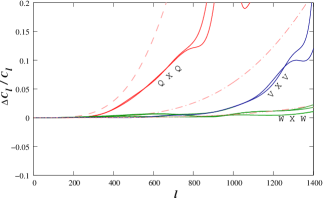
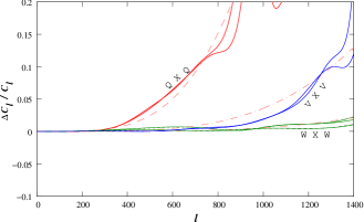
Figure 1: The predicted non-circular beam correction for a CMB experiment with elliptical Gaussian beam with fwhm beam-width of $0.51^{\circ}$ and eccentricity $e:=\sqrt{1-b^{2}/a^{2}}$, where $a$ ($b$) is the semi-major (semi-minor) axis, $e=0.65$ for the Q beam (dashed line), beam-width of $0.35^{\circ}$ and $e=0.46$ for the V beam (dash-dotted line) and beam-width of $0.22^{\circ}$ and $e=0.4$ for the W beam (dash-dot-dot line) are shown in the left plot. The solid curves are the non circular beam corrections estimated by the WMAP team for the Q,V and W channels. In the plot in the right, we show that the non-circular beam correction matches with the estimates of the WMAP team for a slightly different change in the eccentricity of the Q and V beams (W beams matched in the left plot), with the new eccentricities $e=0.50$ and $e=0.40$ respectively. This difference is attributed to the fact that the beams visit the pixels multiple times with different orientations, and hence the effective eccentricity is reduced.

To avoid contamination of the primordial CMB signal by Galactic emission, the region around the Galactic plane is masked from maps. If the Galactic cut is small enough, then the coupling matrix will be invertible, and the two-point correlation function can be determined on all angular scales from the data within the uncut sky (Mortlock et al. 2002). Hivon et al. (2002) present a technique (MASTER) for fast computation of the power spectrum accounting for the galactic cut, but restricted to circular beams. In our present work, we present analytical expressions for the bias matrix of the Pseudo-${C_{l}}$ estimator for the incomplete sky coverage, using a noncircular beam. In Section 2 we show a heuristic approach to the analytic form of the bias matrix taking into account the above mentioned effects. We have shown that our estimation matches with the existing results in different limits in Section 3. In Section 4 we outline the numerical implementation of our approach, estimate the computational cost and suggest a potential algorithmic route to reducing the cost. The discussion and conclusion of this work is given in Section 5.

2 Formalism

The CMB temperature anisotropy field $\Delta T(\mathbf{\hat{q}})$ over all the sky directions $\mathbf{\hat{q}}\equiv(\theta,\phi)$ is assumed to be Gaussian and statistically isotropic and hence the angular power spectrum stores all the statistical information about the anisotropy field. These temperature fluctuations are expanded in the basis of spherical harmonics,

$$\Delta T(\mathbf{\hat{q}})\ =\ \sum_{lm}a_{lm}\,Y_{lm}(\mathbf{\hat{q}}),$$ (1)

where $a_{lm}$ are the spherical harmonic transforms of the temperature anisotropy field

$$a_{lm}\ :=\ \int_{4\pi}d\Omega_{\hat{\mathbf{q}}}\,\Delta T(\mathbf{\hat{q}})\,Y_{lm}^{*}(\mathbf{\hat{q}}).$$ (2)

The observed CMB temperature fluctuation field $\widetilde{\Delta T}(\mathbf{\hat{q}})$ is a convolution of the “beam” profile $B(\mathbf{\hat{q}},\mathbf{\hat{q}^{\prime}})$ with the real temperature fluctuation field $\Delta T(\mathbf{\hat{q}}^{\prime})$ and contaminated by additive experimental noise $n(\mathbf{\hat{q}})$. Moreover, due to the strong influence of the foreground emission in our galactic plane and point sources, some of the pixels have to be masked prior to power spectrum estimation. The mask function $U(\mathbf{\hat{q}})$ is usually assigned zero for the corrupt pixels and one for the clean ones, but it could be a smoother weight function also, that can take values between zero and one, as long as it sufficiently masks the foreground contamination. Mathematically the observed temperature can be expressed as

$$\widetilde{\Delta T}(\mathbf{\hat{q}})\ =\ U(\mathbf{\hat{q}})\left[\int_{4\pi}d\Omega_{\mathbf{\hat{q}^{\prime}}}\,B(\mathbf{\hat{q}},\mathbf{\hat{q}^{\prime}})\,\Delta T(\mathbf{\hat{q}^{\prime}})\ +\ n(\mathbf{\hat{q}})\right].$$ (3)

The spherical harmonic transform of the mask function,

$$U_{lm}\ \equiv\ \int_{4\pi}d\Omega_{\mathbf{\hat{q}}}\,Y_{lm}^{*}({\mathbf{\hat{q}}})\,U(\mathbf{\hat{q}})\,,$$ (4)

is a very useful quantity for our analysis.

Statistical isotropy of underlying CMB anisotropy signal implies that the two point correlation function $C(\mathbf{\hat{q}}_{1},\mathbf{\hat{q}}_{2})=\langle\Delta T(\mathbf{\hat{q}}_{1})\Delta T(\mathbf{\hat{q}}_{2})\rangle$ depends only on the angular separation of the direction, i.e., $C(\mathbf{\hat{q}}_{1},\mathbf{\hat{q}}_{2})=C(\mathbf{\hat{q}}_{1}\cdot\mathbf{\hat{q}}_{2})$. We can therefore expand it as a Fourier-Legendre series

$$\langle\Delta T(\mathbf{\hat{q}}_{1})\Delta T(\mathbf{\hat{q}}_{2})\rangle\ =\ \sum_{l=0}^{\infty}\frac{2l+1}{4\pi}C_{l}\,P_{l}(\mathbf{\hat{q}}_{1}\cdot\mathbf{\hat{q}}_{2}),$$ (5)

where the coefficients $C_{l}$ constitute the CMB power spectrum

$$C_{l}\ \equiv\ \int_{4\pi}d\Omega_{\hat{\mathbf{q}}_{1}}\int_{4\pi}d\Omega_{\hat{\mathbf{q}}_{2}}\langle\Delta T(\mathbf{\hat{q}}_{1})\,\Delta T(\mathbf{\hat{q}}_{2})\rangle\,P_{l}(\mathbf{\hat{q}}_{1}\cdot\mathbf{\hat{q}}_{2}).$$ (6)

The addition theorem for spherical harmonics

$$\frac{4\pi}{2l+1}\sum_{m=-l}^{l}Y_{lm}^{*}(\mathbf{\hat{q}}_{1})\,Y_{lm}(\mathbf{\hat{q}}_{2})\ =\ P_{l}(\mathbf{\hat{q}}_{1}\cdot\mathbf{\hat{q}}_{2}),$$ (7)

and the orthogonality of Legendre polynomials

$$\int_{-1}^{1}dx\,P_{l}(x)\,P_{l^{\prime}}(x)\ =\ \frac{2}{2l+1}\,\delta_{ll^{\prime}}$$ (8)

can then be used to show that the matrix $\langle a_{lm}a_{l^{\prime}m^{\prime}}\rangle$ is diagonal:

$$\langle a_{lm}a_{l^{\prime}m^{\prime}}\rangle\ =\ C_{l}\,\delta_{ll^{\prime}}\,\delta_{mm^{\prime}}.$$ (9)

The observed two point correlation function for a statistically isotropic CMB anisotropy signal is

$$\widetilde{C}(\mathbf{\hat{q}},\mathbf{\hat{q}}^{\prime})=\langle\widetilde{\Delta T}(\mathbf{\hat{q}})\widetilde{\Delta T}(\mathbf{\hat{q}^{\prime}})\rangle=\sum^{\infty}_{l=0}{(2l+1)\over 4\pi}\,C_{l}\,\,W_{l}(\mathbf{\hat{q}},\,\mathbf{\hat{q}}^{\prime})\,,$$ (10)

where $C_{l}$ is the angular power spectrum of CMB anisotropy signal and the window function,

$$W_{l}(\mathbf{\hat{q}}_{1},\mathbf{\hat{q}}_{2})\ :=\ \int d\Omega_{\mathbf{\hat{q}}}\int d\Omega_{\mathbf{\hat{q}^{\prime}}}\,B(\mathbf{\hat{q}}_{1},\mathbf{\hat{q}})B(\mathbf{\hat{q}}_{2},\mathbf{\hat{q}^{\prime}})P_{l}(\mathbf{\hat{q}}\cdot\mathbf{\hat{q}^{\prime}}),$$ (11)

encodes the effect of finite resolution through the beam function. A CMB anisotropy experiment probes a range of angular scales characterized by this window function $W_{l}(\mathbf{\hat{q}},\mathbf{\hat{q}}^{\prime})$. The window depends both on the scanning strategy as well as the angular resolution and response of the experiment. However, it is neater to logically separate these two effects by expressing the window $W_{l}(\mathbf{\hat{q}},\mathbf{\hat{q}}^{\prime})$ as a sum of ‘elementary’ window functions of the CMB anisotropy (Souradeep & Ratra 2001). For a given scanning strategy, the results can be readily generalized using the representation of the window function as a sum over elementary window functions (see, e.g., Souradeep & Ratra 2001, Coble et al. 2003, Mukherjee et al. 2003).

For some experiments, the beam function may be assumed to be circularly symmetric about the pointing direction, i.e., $B(\mathbf{\hat{q}},\mathbf{\hat{q}}^{\prime})\equiv B(\mathbf{\hat{q}}\cdot\mathbf{\hat{q}}^{\prime})$, without significantly affecting the results of the analysis. In any case, this assumption allows a great simplification, since the beam function can then be represented by an expansion in Legendre polynomials as

$$B(\mathbf{\hat{q}}\cdot\mathbf{\hat{q}^{\prime}})\ =\ \frac{1}{4\pi}\,\sum_{l=0}^{\infty}\,(2l+1)\,B_{l}\,P_{l}(\mathbf{\hat{q}}\cdot\mathbf{\hat{q}^{\prime}}),$$ (12)

where,

$$B_{l}\equiv\int_{-1}^{1}d(\mathbf{\hat{q}}\cdot\mathbf{\hat{q}^{\prime}})\,P_{l}(\mathbf{\hat{q}}\cdot\mathbf{\hat{q}^{\prime}})\,\mathcal{B}(\mathbf{\hat{q}}\cdot\mathbf{\hat{q}^{\prime}}),$$ (13)

and $\mathcal{B}(\mathbf{\hat{q}}\cdot\mathbf{\hat{q}^{\prime}})$ is the circularized beam obtained by averaging $B(\mathbf{\hat{z}},\mathbf{\hat{q}})$ over the azimuthal coordinate $\phi$. Consequently, it is straightforward to derive the well known simple expression

$$W_{l}(\mathbf{\hat{q}},\,\mathbf{\hat{q}^{\prime}})\ =\ B^{2}_{l}\,P_{l}(\mathbf{\hat{q}}\cdot\mathbf{\hat{q}^{\prime}})\,,$$ (14)

for a circularly symmetric beam function. For non-circular beams and incomplete sky coverage the Pseudo-$C_{l}$ estimator,

$$\widetilde{{C}}_{l}\ \equiv\ \frac{1}{2l+1}\sum_{m=-l}^{l}\left|\widetilde{a}_{lm}\right|^{2},$$ (15)

takes the form

$$\widetilde{{C}}_{l}\ =\ \frac{1}{4\pi}\int_{4\pi}d\Omega_{\mathbf{\hat{q}}_{1}}\int_{4\pi}d\Omega_{\mathbf{\hat{q}}_{2}}\,U(\mathbf{\hat{q}}_{1})\,U(\mathbf{\hat{q}}_{2})\,P_{l}(\mathbf{\hat{q}}_{1}\cdot\mathbf{\hat{q}}_{2})\,\widetilde{\Delta T}(\mathbf{\hat{q}}_{1})\,\widetilde{\Delta T}(\mathbf{\hat{q}}_{2}).$$ (16)

In this case, the expectation value of the Pseudo-$C_{l}$ estimator becomes

$$\langle\widetilde{\mathcal{C}}_{l}\rangle\ =\ \sum_{{l^{\prime}}}A_{l{l^{\prime}}}C_{l^{\prime}}\ +\ \bar{C}_{l}^{N},$$ (17)

that is, the estimator is non-trivially biased, where the bias matrix $A_{l{l^{\prime}}}$ takes the form

$$A_{l{l^{\prime}}}=\frac{1}{2l+1}\sum_{n=-l}^{l}\!\sum_{m=-{l^{\prime}}}^{l^{\prime}}\!\left|\int_{4\pi}\!\!\!d\Omega_{\mathbf{\hat{q}}}U(\mathbf{\hat{q}})\,Y_{ln}(\mathbf{\hat{q}})\left[\int_{4\pi}\!\!\!d\Omega_{\mathbf{\hat{q}^{\prime}}}\,Y^{*}_{{l^{\prime}}m}(\mathbf{\hat{q}^{\prime}})\,B(\mathbf{\hat{q}},\mathbf{\hat{q}^{\prime}})\right]\right|^{2}.$$ (18)

The noise term $\bar{C}_{l}^{N}$, arising from instrumental noise, can be measured to a very high accuracy. If the noise term for full sky coverage $C_{l}^{N}$ is known, it can be combined with the bias matrix for incomplete sky coverage $M_{l{l^{\prime}}}$ (Hivon et al. 2002) to obtain the noise power spectrum for cut-sky $\bar{C}_{l}^{N}$

$$\bar{C}_{l}^{N}\ =\ \sum_{{l^{\prime}}}M_{l{l^{\prime}}}\,C_{l^{\prime}}^{N},$$ (19)

where, $M_{l{l^{\prime}}}$ is defined as

$$M_{l{l^{\prime}}}\ =\,\frac{2l^{\prime}+1}{4\pi}\sum_{l^{\prime\prime}=|l-l^{\prime}|}^{l+l^{\prime}}\,(2l^{\prime\prime}+1)\,{\left(\begin{array}[]{lcr}l&l^{\prime}&l^{\prime\prime}\\ 0&0&0\end{array}\right)}^{2}\,{\cal{U}}_{l^{\prime\prime}},$$ (20)

with ${\cal{U}}_{{l^{\prime\prime}}}\equiv\sum_{m^{\prime\prime}=-{l^{\prime\prime}}}^{{l^{\prime\prime}}}|U_{{l^{\prime\prime}}m^{\prime\prime}}|^{2}/(2{l^{\prime\prime}}+1)$. Computation of the bias matrix is important for defining the unbiased Pseudo-$C_{l}$ estimator

$$\widetilde{C}_{l}^{\rm{UB}}\ \equiv\ \sum_{{l^{\prime}}}[A^{-1}]_{l{l^{\prime}}}\,\left(\widetilde{C}_{l^{\prime}}\ -\ \sum_{{l^{\prime\prime}}}M_{{l^{\prime}}{l^{\prime\prime}}}\,C_{l^{\prime\prime}}^{N}\right)$$ (21)

that removes the systematic effects of beam non-circularity and incomplete sky coverage.

The experimental beams in CMB experiments are mildly non-circular, and hence it makes sense to define Beam Distortion Parameters (BDP) $\beta_{lm}(\ll 1)$ so that we can calculate the result in a perturbative expansion of small parameter. The BDP $\beta_{lm}$ is expressed as $\beta_{lm}\equiv b_{lm}/b_{l0}$, where the $b_{lm}$ are the spherical harmonic moments of the beam function for the pointing direction $\mathbf{\hat{z}}$:

$$b_{lm}\equiv\int_{4\pi}d\Omega_{\mathbf{\hat{q}}}\,Y_{lm}^{*}({\mathbf{\hat{q}}})\,B(\mathbf{\hat{z}},\mathbf{\hat{q}})\,,$$ (22)

and $B_{l}$, defined in Eq. (13), is connected to $b_{l0}$ through the relation:

$$B_{l}=\int_{0}^{\pi}\sin\theta d\theta\,\sqrt{\frac{4\pi}{2l+1}}\,Y_{l0}^{*}({\mathbf{\hat{q}}})\left[\frac{1}{2\pi}\int_{0}^{2\pi}d\phi\,B(\mathbf{\hat{z}},\mathbf{\hat{q}})\right]=\sqrt{\frac{4\pi}{2l+1}}\,b_{l0}.$$

Evaluation of the spherical harmonic transforms of the beam function $B(\mathbf{\hat{q}},\mathbf{\hat{q}^{\prime}})$ for each pointing direction $\mathbf{\hat{q}}$ is computationally prohibitive. We use the spherical harmonic transforms $b_{lm}$ of $B(\hat{\mathbf{z}},\mathbf{\hat{q}^{\prime}})$, incorporating rotation in it via Wigner-$D$ functions, in order to compute the harmonic transforms of $B(\mathbf{\hat{q}},\mathbf{\hat{q}^{\prime}})$ for any $\mathbf{\hat{q}}$ by using the formula [42]

$$\int_{4\pi}d\Omega_{\mathbf{\hat{q}^{\prime}}}\,Y^{*}_{{l^{\prime}}m}(\mathbf{\hat{q}^{\prime}})\,B(\mathbf{\hat{q}},\mathbf{\hat{q}^{\prime}})\ =\ \sqrt{\frac{2{l^{\prime}}+1}{4\pi}}\sum_{m^{\prime}=-{l^{\prime}}}^{l^{\prime}}B_{l^{\prime}}\,\beta_{{l^{\prime}}m^{\prime}}\,D^{l^{\prime}}_{mm^{\prime}}(\mathbf{\hat{q}},\rho(\mathbf{\hat{q}})).$$ (23)

Then, using the spherical harmonic expansion of the mask function $U(\mathbf{\hat{q}})$

$$U(\mathbf{\hat{q}})\ =\ \sum_{l=0}^{\infty}\sum_{m=-l}^{l}U_{lm}\,Y_{lm}(\mathbf{\hat{q}}),$$ (24)

we can rewrite the general form of the bias matrix [Eq. (18)] as

$$A_{ll^{\prime}}\ =\ \frac{B_{l}^{2}}{4\pi}\frac{(2l^{\prime}+1)}{(2l+1)}\sum_{n=-l}^{l}\sum_{m=-l^{\prime}}^{l^{\prime}}\left|\sum_{m^{\prime}=-l^{\prime}}^{l^{\prime}}\beta_{l^{\prime}m^{\prime}}\sum_{{l^{\prime\prime}}=0}^{\infty}\sum_{m^{\prime\prime}=-{l^{\prime\prime}}}^{{l^{\prime\prime}}}U_{{l^{\prime\prime}}m^{\prime\prime}}\,J^{l{l^{\prime\prime}}{l^{\prime}}}_{nm^{\prime\prime}mm^{\prime}}\right|^{2},$$ (25)

where

$$J^{l{l^{\prime\prime}}{l^{\prime}}}_{nm^{\prime\prime}mm^{\prime}} := \int_{4\pi}d\Omega_{\mathbf{\hat{q}}}\,Y_{ln}(\mathbf{\hat{q}})\,Y_{{l^{\prime\prime}}m^{\prime\prime}}(\mathbf{\hat{q}})\,D_{mm^{\prime}}^{l^{\prime}}(\mathbf{\hat{q}},\rho(\mathbf{\hat{q}}))$$ (27)

$$= (-1)^{n+m^{\prime\prime}}\frac{\sqrt{(2l+1)(2{l^{\prime\prime}}+1)}}{4\pi}\sum_{L=|l-{l^{\prime\prime}}|}^{l+{l^{\prime\prime}}}C^{L0}_{l0{l^{\prime\prime}}0}\,C^{L(n+m^{\prime\prime})}_{ln{l^{\prime\prime}}m^{\prime\prime}}\times$$

$$\sum_{{L^{\prime}}=|L-{l^{\prime}}|}^{L+{l^{\prime}}}C^{{L^{\prime}}(m-n-m^{\prime\prime})}_{L(-n-m^{\prime\prime}){l^{\prime}}m}\,C^{{L^{\prime}}m^{\prime}}_{L0{l^{\prime}}m^{\prime}}\,\chi^{L^{\prime}}_{(m-n-m^{\prime\prime})m^{\prime}}[\rho(\mathbf{\hat{q}})]$$

and

$$\chi^{l}_{mm^{\prime}}[\rho(\mathbf{\hat{q}})]\ :=\ \int_{4\pi}d\Omega_{\mathbf{\hat{q}}}\,D^{l}_{mm^{\prime}}(\mathbf{\hat{q}},\rho(\mathbf{\hat{q}})).$$ (28)

To obtain the expression for the $J$ coefficients above we have introduced Clebsch Gordon coefficients $C^{ll^{\prime}}_{m_{1}m_{2}m^{\prime}_{1}m^{\prime}_{2}}$ along with sinusoidal expansion of Wigner-$d$ (see Appendix A.1 for details).

Eq. (27) provides the expression for the bias [Eq. (25)] in its full generality. For a specified general form of the scan strategy, however, we need to precompute the coefficients $\chi^{l}_{mm^{\prime}}$ which are functionals of $\rho(\mathbf{\hat{q}})$. Special cases, which often provide good approximations to the real scan strategies, provide significant computational advantages. From the definition of $\chi$ coefficients we show below that

1. For a $\rho(\mathbf{\hat{q}})$ separable in declination and Right Ascension parts, i.e. $\rho(\mathbf{\hat{q}})\equiv\Theta(\theta)+\Phi(\phi)$,

   $$\chi^{l}_{mm^{\prime}}[\rho(\mathbf{\hat{q}})]\ =\ \int_{0}^{2\pi}d\phi\,e^{-im\phi}\,e^{-im^{\prime}\Phi(\phi)}\int_{0}^{\pi}\sin\theta\,d\theta\,d^{l}_{mm^{\prime}}(\theta)\,e^{-im^{\prime}\Theta(\theta)}$$ (29)

   would have significant values only in a much constrained domain of the indices $m,m^{\prime}$.

2. For equal declination scan strategies, where $\rho(\mathbf{\hat{q}})\equiv\rho(\theta)$, we show below that the computational cost reduces to that of the non-rotating beam ($\rho(\mathbf{\hat{q}})=0$) case.

Hence, the study of the bias computation for non-rotating beams provides an analytic framework that is computationally equivalent to a broader class of scan strategies as mentioned at the appropriate places below.

It is clear from the definition of $\chi^{l}_{mm^{\prime}}$ that for equal declination scans [case II] the $\phi$ integral is leading to the constraint

$$\chi^{l}_{mm^{\prime}}[\rho(\mathbf{\hat{q}})=0]\propto\int_{0}^{2\pi}d\phi\,e^{im\phi}\ =\ 2\pi\,\delta_{m0}.$$ (30)

So the $J$ coefficients in Eq. (27) contribute to bias only when $m^{\prime\prime}=m-n$, saving huge amount of computation. For a much broader class within case I, it is reasonable to expect that the $\chi$ symbols in the final expression for bias will contribute when $m^{\prime\prime}$ is close to $m-n$.

For equal declination scan strategies, the expression for the bias matrix can be written as

$$A_{ll^{\prime}} = B_{l}^{2}\,\frac{(2{l^{\prime}}+1)}{16\pi}\sum_{n=-l}^{l}\sum_{m=-l^{\prime}}^{l^{\prime}}\left|\sum_{{l^{\prime\prime}}=0}^{\infty}\sqrt{2{l^{\prime\prime}}+1}\,U_{{l^{\prime\prime}}(m-n)}\right.\ \times$$ (31)

$$\sum_{L=|l-{l^{\prime\prime}}|}^{l+{l^{\prime\prime}}}C^{L0}_{l0{l^{\prime\prime}}0}\,C^{Lm}_{ln{l^{\prime\prime}}(m-n)}\sum_{{L^{\prime}}=|L-{l^{\prime}}|}^{L+{l^{\prime}}}C^{{L^{\prime}}0}_{L-m{l^{\prime}}m}\sum_{N=-{L^{\prime}}}^{{L^{\prime}}}d^{{L^{\prime}}}_{0N}\left(\frac{\pi}{2}\right)\ \times$$

$$\left.\sum_{m^{\prime}=-l^{\prime}}^{l^{\prime}}\beta_{l^{\prime}m^{\prime}}\,C^{{L^{\prime}}m^{\prime}}_{L0{l^{\prime}}m^{\prime}}\,d^{{L^{\prime}}}_{Nm^{\prime}}\left(\frac{\pi}{2}\right)\,\Gamma_{m^{\prime}N}[\rho(\theta)]\right|^{2},$$

where the coefficients

$$\Gamma_{m^{\prime}N}[\rho(\theta)]\ :=\ i^{m^{\prime}}\,(-1)^{N}\int_{0}^{\pi}\sin\theta d\theta\,e^{iN\theta}\,e^{-im^{\prime}\rho(\theta)}$$ (32)

are functionals of the scan strategy and have to be precomputed (analytically/numerically) for a given $\rho(\theta)$.

For an efficient computation of the $J$ coefficients using a numerical implementation scheme described in section 4, we derive an alternative expression for the $J$ coefficients using the sinusoidal expansion of Wigner-$d$ that only involves the $d^{l}_{mm^{\prime}}(\pi/2)$ symbols (see Appendix A.2 for details):

$$J^{l{l^{\prime\prime}}{l^{\prime}}}_{nm^{\prime\prime}mm^{\prime}} = \frac{\sqrt{(2l+1)(2{l^{\prime\prime}}+1)}}{4\pi}\,i^{n+m+m^{\prime\prime}}\sum_{M=-l}^{l}d^{l}_{nM}\left(\frac{\pi}{2}\right)\,d^{l}_{M0}\left(\frac{\pi}{2}\right)\times$$ (33)

$$\sum_{{M^{\prime\prime}}=-{l^{\prime\prime}}}^{{l^{\prime\prime}}}d^{{l^{\prime\prime}}}_{m^{\prime\prime}{M^{\prime\prime}}}\left(\frac{\pi}{2}\right)\,d^{{l^{\prime\prime}}}_{{M^{\prime\prime}}0}\left(\frac{\pi}{2}\right)\sum_{M^{\prime}=-{l^{\prime}}}^{{l^{\prime}}}d^{{l^{\prime}}}_{mM^{\prime}}\left(\frac{\pi}{2}\right)\,d^{{l^{\prime}}}_{M^{\prime}m^{\prime}}\left(\frac{\pi}{2}\right)\,\Xi_{(M+M^{\prime}+M^{\prime\prime})(m^{\prime\prime}-m+n)m^{\prime}}$$

where the coefficients,

$$\Xi_{m_{1}m_{2}m_{3}}\ :=\ (-1)^{m_{1}}\,i^{m_{3}}\int_{0}^{2\pi}d\phi\,e^{im_{2}\phi}\int_{0}^{\pi}\sin\theta d\theta\,e^{im_{1}\theta}\,e^{-im_{3}\rho(\mathbf{\hat{q}})},$$ (34)

have to be precomputed for a given scan strategy. Since the above expression [Eq. (33)] provides just an alternate form for the most general expression for bias, the discussion on different special cases given after Eq. (27) also holds here. Thus, in case I [$\rho(\mathbf{\hat{q}})\equiv\Theta(\theta)+\Phi(\phi)$] the $\Xi$ coefficients would take the form

$$\Xi_{m_{1}m_{2}m_{3}}\ :=\ (-1)^{m_{1}}\,i^{m_{3}}\int_{0}^{2\pi}d\phi\,e^{im_{2}\phi}\,\,e^{-im_{3}\Phi(\phi)}\int_{0}^{\pi}\sin\theta d\theta\,e^{im_{1}\theta}\,e^{-im_{3}\Theta(\theta)},$$ (35)

which are likely to contribute significantly for a highly constrained set of $m_{1},m_{2},m_{3}$ values and in case II (equal declination scans) $\Xi_{m_{1}m_{2}m_{3}}$ contributes only for $m_{2}=0$, so the expression for the bias matrix becomes

$$A_{ll^{\prime}} = B_{l}^{2}\,\frac{(2{l^{\prime}}+1)}{16\pi}\sum_{n=-l}^{l}\sum_{m=-l^{\prime}}^{l^{\prime}}\left|\sum_{{l^{\prime\prime}}=0}^{\infty}\sqrt{2{l^{\prime\prime}}+1}\,U_{{l^{\prime\prime}}(m-n)}\right.\ \times$$ (36)

$$\sum_{{M^{\prime\prime}}=-{l^{\prime\prime}}}^{{l^{\prime\prime}}}d^{{l^{\prime\prime}}}_{(m-n){M^{\prime\prime}}}\left(\frac{\pi}{2}\right)\,d^{{l^{\prime\prime}}}_{{M^{\prime\prime}}0}\left(\frac{\pi}{2}\right)\sum_{M=-l}^{l}d^{l}_{nM}\left(\frac{\pi}{2}\right)\,d^{l}_{M0}\left(\frac{\pi}{2}\right)\ \times$$

$$\left.\sum_{M^{\prime}=-{l^{\prime}}}^{{l^{\prime}}}d^{{l^{\prime}}}_{mM^{\prime}}\left(\frac{\pi}{2}\right)\sum_{m^{\prime}=-l^{\prime}}^{l^{\prime}}\beta_{l^{\prime}m^{\prime}}\,d^{{l^{\prime}}}_{M^{\prime}m^{\prime}}\left(\frac{\pi}{2}\right)\,\Gamma_{m^{\prime}(M+M^{\prime}+M^{\prime\prime})}[\rho(\theta)]\right|^{2}.$$

Here we have use the same $\Gamma$ coefficients as defined in Eq. (32). In most of the cases, the beam pattern and the scan strategies have trivial symmetries, where only the real parts of the $\Gamma$ coefficients contribute.

The case of non-rotating beams, $\rho(\mathbf{\hat{q}})=0$, has been explicitly worked out in Appendix B. This is a specific example where the real part of the $\Gamma$ symbols can be written in a closed form and the result is:

$$\Re\left[\Gamma_{m^{\prime}N}[\rho(\mathbf{\hat{q}})=0]\right]\ =:\ f_{m^{\prime}N}\ =\ \left\{\begin{array}[]{cl}(-1)^{(m^{\prime}\pm 1)/2}\,\pi/2&\mbox{if $m^{\prime}=odd$ and $N=\pm 1$}\\ (-1)^{m^{\prime}/2}\,2/(1-N^{2})&\mbox{if both $m^{\prime},N=0$ or $even$}\\ 0&\mbox{otherwise.}\end{array}\right.$$ (37)

So in order to compute the bias matrix for non-rotating beams, only the $\Gamma$ symbols in Eqs. (31) or (36) have to be replaced by the above $f$ symbols. We thus arrive at the important conclusion that the computation cost for estimating the bias for equal declination scans is the same as that for non-rotating beams (only the precomputed $\Gamma$ coefficients for that scan strategy would be required). It is also reasonable to expect that the computation cost would be of the same order even for a broader class of scan strategies (e.g., as in case I) which can provide reasonable approximations to the real scan strategies.

3 Limiting cases: Circular beam with full sky coverage & incomplete sky coverage

The analytic expressions for bias derived in the previous section reduce to the known analytical results for non-uniform sky coverage with circular beams studied in Hivon et al. (2002) and our earlier results for the leading order effect of non-rotating noncircular beams with full sky coverage (Mitra et al. 2004).

The special cases of circular beam and/or complete sky coverage limits are readily recovered from our general expressions.

First, the simplest case of complete sky coverage with circular beam limit can be obtained by substituting $U_{lm}=\sqrt{4\pi}\delta_{l0}$ and $\beta_{lm}=\delta_{m0}$. We show in the Appendix C.1 that we get back the well known result

$$A_{ll^{\prime}}\ =\ B_{l}^{2}\,\delta_{ll^{\prime}}.$$

Hivon et al. (2002) formulated MASTER (Monte Carlo Apodized Spherical Transform Estimator) method for the estimation of CMB angular power spectrum from ‘cut’ (incomplete) sky coverage for circular beams. Substituting the circular beam limit [$\beta_{lm}\delta_{m0}$] in the expression for bias matrix we recover the MASTER circular beam result in Appendix C.2:

$$A_{ll^{\prime}}\ =\ B_{l}^{2}\,\frac{2l^{\prime}+1}{4\pi}\sum_{l^{\prime\prime}=|l-l^{\prime}|}^{l+l^{\prime}}\,(2l^{\prime\prime}+1)\,{\left(\begin{array}[]{lcr}l&l^{\prime}&l^{\prime\prime}\\ 0&0&0\end{array}\right)}^{2}\,{\cal{U}}_{l^{\prime\prime}},$$ (38)

where ${\cal{U}}_{{l^{\prime\prime}}}\equiv\sum_{m^{\prime\prime}=-{l^{\prime\prime}}}^{{l^{\prime\prime}}}|U_{{l^{\prime\prime}}m^{\prime\prime}}|^{2}/(2{l^{\prime\prime}}+1)$.

Finally, in Appendix C.3, we recover the general formula for leading order correction with full sky coverage for noncircular beams presented in Mitra et al. (2004). We substitute $U_{lm}=\sqrt{4\pi}\delta_{l0}$ in the expression for the bias matrix and get back

$$A_{ll^{\prime}}\ =\ B_{l}^{2}\,\frac{(2l^{\prime}+1)}{4}\sum_{m=-\rm{min}(l,l^{\prime})}^{\rm{min}(l,l^{\prime})}\left|\sum_{m^{\prime}=-l^{\prime}}^{l^{\prime}}\beta_{l^{\prime}m^{\prime}}\,\int_{-1}^{1}d\cos\theta\,d^{l}_{m0}(\theta)\,d^{l^{\prime}}_{mm^{\prime}}(\theta)\right|^{2}.$$ (39)

Note that due to a somewhat different definition of bias matrix in Mitra et al. (2004), for $\mathcal{C}_{l}\equiv[l(l+1)/(8\pi^{2})]C_{l}$, the results differ by a factor of $[l^{\prime}(l^{\prime}+1)]/[l(l+1)]$ from Eq. (38) of Mitra et al. (2004). Unfortunately, the complex form of the final expression for leading order correction to bias matrix with non-rotating beams presented in Eq. (43) of Mitra et al. (2004), does not allow an explicit comparison of the results term by term.

4 Numerical Implementation

The main motivation for deriving the analytic results is to evade the computational cost and the time taken to estimate the bias using end to end simulations. The present work takes us one step ahead. The analysis framework we have developed can now estimate the effect of non-circular beams including the effect of non-uniform sky coverage for any given scan strategy. However, the numerical evaluation of the algebraic expression for the bias matrix derived in section 2 is also a computational challenge. As discussed in section 2, for a broad class of scan strategies, which often provide good approximations to real scan strategies (e.g., WMAP [23]), the computational cost for bias estimation can be significantly reduced to the same order as needed for equal declination scan strategies. More importantly, in situations where a iso-declination scan strategy only provides a crude approximation (e.g., Planck), the resulting bias estimate can be useful to judge the severity of the asymmetric beam effect and, hence, to decide at which level of rigor the problem needs to be addressed in the analysis pipeline development.

In this section we describe the detailed computation scheme for equal declination scan strategies and show that the computational cost is within reach. We also suggest certain criteria for the choice of the masks in order to reduce the computational burden. Though the implementation of our analysis can be computationally expensive in the most general cases, even then the importance of this method can not be underestimated. This analysis can illuminate several “shortcuts” in the end-to-end simulations to reduce the computational cost; furthermore, it has the potential to eventually replace the end-to-end simulation entirely.

4.1 Fast computation of the bias matrix

Our scheme for fast computation of the bias is based on the alternate form of the bias expressed by Eq. (36). Possibility of fast computation of the form given by the combination of Eqs. (25) and (27) is being considered.

The final analytic form of the bias matrix for equal declination scans, given by Eq. (36), contains infinite summations. These summations have to be truncated for given accuracy goals using reasonable physical insights. Let us denote the ($l,m$) cut-offs for the mask and beam by ($l_{\rm{mask}},m_{\rm{mask}}$) and ($l_{\rm{beam}},m_{\rm{beam}}$) respectively. The choice of the numerical values for these cut-offs will be provided in the numerical results section.

Computation of the final expression by naively implementing the analytic expression given by Eq. (36) is expensive. Three major innovations have been introduced in order to numerically evaluate the bias matrix:

1. We used a smart implementation of the hierarchical summations to reduce the computational cost by a few orders of magnitude. To calculate three coupled loops of the form

   $$S=\sum_{i=1}^{N}\sum_{j=1}^{N}\sum_{k=1}^{N}f(i+j+k),$$ (40)

   naively $N^{3}$ operations seem necessary. However, if we calculate the summation in the following order:

   $$V(m) := \sum_{k=1}^{N}f(m+k);\ \ \ m=1,2,\ldots,2N$$ (41)

   $$S = \sum_{i=1}^{N}\sum_{j=1}^{N}V(i+j)$$ (42)

   we effectively require just $2N^{2}+N^{2}=3N^{2}$ operations. The computational gain is $N/3$. For $N=3000$, this factor is 1000. This example is for a very simple case where all the summations have the same limits, but clearly this can be extended to the case of summations with unequal limits and match our analysis (See Appendix D for details). Here the summations within the modulus symbols in (36) (that is for each set of $l,l^{\prime},m,n$) are computed in three stages:

   • Step I:

     $$V^{1}(N)\ =\ \sum_{M^{\prime}=-l^{\prime}}^{l^{\prime}}d^{l^{\prime}}_{mM^{\prime}}\left(\frac{\pi}{2}\right)\sum_{m^{\prime}=-m_{\rm{beam}}}^{m_{\rm{beam}}}\beta_{l^{\prime}m^{\prime}}\,d^{l^{\prime}}_{M^{\prime}m^{\prime}}\left(\frac{\pi}{2}\right)\,\Gamma_{m^{\prime}(M^{\prime}+N)}[\rho(\theta)]$$ (43)

     $N$ runs from $-(l+m_{\rm{mask}})$ to $+(l+m_{\rm{mask}})$

   • Step II:

     $$V^{2}(M^{\prime\prime})\ =\ \sum_{M=-l}^{l}d^{l}_{nM}\left(\frac{\pi}{2}\right)\,d^{l}_{M0}\left(\frac{\pi}{2}\right)\,V^{1}(M+M^{\prime\prime})$$ (44)

   • Step III:

     $$V^{3} = \sum_{l^{\prime\prime}=0}^{l_{\rm{mask}}}\sqrt{2l^{\prime\prime}+1}\,U_{l^{\prime\prime}(m-n)}\ \times$$ (45)

     $$\sum_{M^{\prime\prime}=-m_{\rm{mask}}}^{m_{\rm{mask}}}d^{l^{\prime\prime}}_{(m-n)M^{\prime\prime}}\left(\frac{\pi}{2}\right)d^{l^{\prime\prime}}_{M^{\prime\prime}0}\left(\frac{\pi}{2}\right)V^{2}(M^{\prime\prime})$$

   For $l_{\rm{beam}}=l_{\rm{max}}$ the computation time with naive implementation would scale as $\sim(8/3)(2m_{\rm{mask}}+1)(2m_{\rm{beam}}+1)l_{\rm{max}}^{5}l_{\rm{mask}}^{2}$, whereas the above algorithm reduces the computation cost to $\sim(4/3)(2m_{\rm{mask}}+1)(2m_{\rm{beam}}+1)l^{5}_{\rm{max}}$, providing a speed-up factor of $\sim 2l_{\rm{mask}}^{2}$.

   Mildly non-circular beams, where the BDP $\beta_{lm}$ at each $l$ falls off rapidly with $m$, allows us to neglect $\beta_{lm}$ for $m>m_{\rm{beam}}$. For most realistic beams, $m_{\rm{beam}}\sim 4$ is a sufficiently good approximation (Souradeep & Ratra 2001) and this cuts off the summation over BDP in the bias matrix $A_{l{l^{\prime}}}$.

   Soft, azimuthally apodized, masks where the coefficients $U_{lm}$ are small beyond $m>m_{\mathrm{mask}}$, similarly allows us to truncate the sum involving $U_{lm}$. Moreover, it is useful to smooth the mask in $l$, such the $U_{lm}$ die off rapidly for $l>l_{\mathrm{mask}}$ too.

   Clearly, small values of ${m_{\rm{beam}}}$ and ${m_{\rm{mask}}}$ lead to computational speed up. Detailed discussion on mask making is shown in section 4.2.

2. The Wigner-$d$ functions with argument $\pi/2$ occur too frequently in the above evaluation. So one possibility to reduce computation cost was to pre-compute all the Wigner-$d$ coefficients $d^{l}_{mn}(\pi/2)$ at once. But for $l\sim 1000$ this scheme is limited by disk/memory storage and/or program Input/Output (I/O) overhead.

   However, we may observe that, in each step of computation described in Eq. (45) only one value of $l$ occurs in the $d$ symbols with the same argument $\pi/2$. Hence we use an efficient recursive routine presented in Risbo (1996) that generates all the $d^{l}_{mn}(\pi/2)$ at once for a given value of $l$. This allows us to compute the Wigner-$d$ symbols efficiently and use them as constant coefficients at each step without any significant I/O limited operations.

3. There are several symmetries involved in the spherical harmonic transforms and the Wigner-$d$ symbols, which could be utilized to get more than an order of magnitude reduction in the computation time.

4. Finally, we know that the bias matrix is not far off from diagonal, because the beams are mildly non-circular (see the plots of bias matrices in [31]). So we need not compute all the elements of the bias matrix. Rather, a diagonal band (could be of triangular shape) of average “thickness” $\Delta l$ can be used to calculate the $C_{l}$ estimation error with a fairly high accuracy. This will give an additional speed-up factor of $\sim l/\Delta l$.

While speeding up the numerical implementation of the above analysis is under progress, the estimate of computational requirement for the basic code for $l_{\rm{max}}=3000$ is quite promising, well within the computing resources available to the CMB community (see sec. 4.3 for details).

It is also interesting to note here that for different models of the same beam, which would at most differ at a highly constrained band in the harmonic space, the bias computation needs to be repeated only for those harmonic components. This would save large amount of computation. This advantage may not be available to pixel based end to end Monte Carlo simulation methods for estimating bias.

4.2 Constructing azimuthally apodized masks

The temperature anisotropies observed by any detector are combinations of CMB as well as foreground. The dominant contribution of foreground arises from the galactic plane. While methods of foreground removal using multi-wavelength observations exist, there is significant residual along the galactic plane to require masking of that region prior to cosmological power spectrum estimation. The mask is designed to remove the effect of regions of excessive galactic emission and spots around strong extragalactic radio sources (Bennett et al. 2003b, Saha et al. 2006).

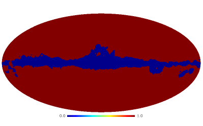
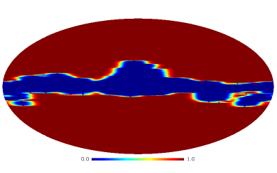
Figure 2: The KP2 original mask (left) and the azimuthally smoothed mask reconstructed from the KP2 mask (right).

The effect of masked map on the angular power spectrum estimation has been described in the literature (Hivon et al. 2002). However, as we have shown, the effect of cut sky becomes nontrivial for a non-circular beam function. The sum over all the $U_{lm}$ modes of the mask is responsible for the large additional computation cost. In particular, our computational cost estimate in the previous subsection shows that a mask that allows us to choose a modest value of $m_{\rm{mask}}$ leads to a proportionally smaller computational cost. A mask whose transform is such that power in high $m$ modes for a given $l$ is suppressed would clearly serve this purpose (Souradeep et al., 2006).

To achieve this we propose a possible method for generating an azimuthally-apodized version of a given mask  as outlined in the following steps:

1. We compute spherical harmonic coefficients $U_{lm}$ of the original mask $U^{o}(\hat{q})$. We directly suppress the power at high $m$, by re-scaling

   $$U^{\prime}_{lm}=\exp{(-m*m/[\alpha\,{m_{\rm{mask}}}^{2}])}*U_{lm}$$ (46)

   corresponding to smoothing the mask along the azimuthal direction. Where $\alpha$ determines the extent to which power is suppressed at the given cut-off value of $m_{\rm{mask}}$.

2. The re-scaled $U_{lm}$ are transformed to make an auxiliary mask $U^{\prime}(\hat{q})$.

3. However, it is clear that mask $U^{\prime}(\hat{q})$ would allow power from contaminated regions. We should ensure that all regions where $U^{o}(\hat{q})=0$ remain zero. A simple way to do that would be to multiply $U^{\prime}(\hat{q})$ with $U^{o}(\hat{q})$ in the pixel space. Hence, we define the final apodized mask as

   $$U^{a}(\hat{q})=[U^{\prime}(\hat{q})]^{s}\,U^{o}(\hat{q}),$$ (47)

   where $s$ is a sufficiently large number ($\alpha=1$, $m_{\rm{mask}}=10$ and $s=12$ in our example shown in figures 2 & 3) to ensure that the edges of the final mask are smoothed to the required level. To be more explicit, multiplying $U^{\prime}$ with $U_{0}$ would introduce steps in the mask. Raising $U^{\prime}$ to be a sufficiently high power ensures that the amplitude of the step is reduced.

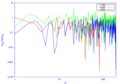
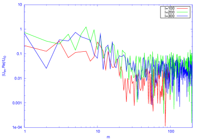
Figure 3: $U_{lm}$s of the original mask KP2 (left) and the mask Kp2^′ (right).

The final mask obtained in this method is shown in the right panel of figure 2. We extract $U_{lm}$ from this final mask $U^{a}(\hat{q})$. We show the $U_{lm}$ of the original mask KP2 and the azimuthally apodized mask Kp2^a in figure 3. Clearly, the later show very rapid decrease of a mode with $m$ for a given $l$. In the example shown here, we have significant contribution only from the first 10-20 $m$ modes, for a given $l$. The $|U_{lm}|^{2}$ also dies down with $l$ allowing us also to put a cut-off at $l=l_{\rm{mask}}\sim 100$. A reconstructed mask following this method has the advantage that it reduces the computation time for bias matrix by a large factor.

4.3 Estimate of time for calculating the Bias matrix

We have (semi)empirically estimated the CPU time required by our codes for equal declination scan strategies with apodized masks. Since the computation cost for equal declination scan strategies is the same as that for non-rotating beams, we use the latter for simplicity.

We ran our codes for maximum multipoles $l_{\rm{max}}$ of 50, 60, 65, 70, 75, 85, 90 & 100 in a 8 processor (4$\times$ AMD Opteron Dual core at 2.6 Ghz) node and having 16 GB of RAM. The recorded computation times are shown in the log - log plot in figure 4 (circled points). We fitted these points with linear functions of the form $y(x)=\alpha x+\beta$. The best fit is obtained for $\beta=-7.6$ and $\alpha=5.5$ (dotted line), which indicates that the observed computation time scales as $l^{5.5}$, whereas algorithmically we show that it should be $l^{5}$. While the theoretical prediction (dashed line) is also quite close to the observed values, the discrepancy is perhaps related to the simplistic implementation we have used in our codes and this difference should reduce in near future as the code evolves.

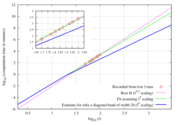
Figure 4: Circled points are the datapoints of the sample time for running the code at different multipoles. The dotted line is the best fit curve. The dashed line is the theoretically expected estimate for the full bias matrix. The solid line below is the estimated computation will be required if we consider only a diagonal band of width $\Delta l$ = 20 elements in the bias matrix elements where the effect of non-circular beams is significant.

Further reduction of computation is conceivable in the future:

1. If we take into account that the bias matrix is most significant only along a narrow strip (approximately $\Delta l$ = 20 elements wide on average and not necessarily uniform - could be wedge shaped) around the diagonal of the bias matrix, the time estimate reduces by another power of $l$. The solid line in Figure 4 refers to the plot of estimated computation time against multipole in the log scale, with the slope reduced by 1 (i.e. 5-1=4). When $l_{\rm{max}}\leq 20$, of course, there is no reduction in computation cost, which is shown by the first part of the solid curve.

2. Using the symmetries of the Wigner-d symbols, it is possible to reducing the computation cost by more than an order of magnitude.

If all the above modifications are implemented, the bias calculation is expected to be feasible in quite reasonable time with the computing facilities available/dedicated to the CMB community. For example, with 1000 dual core CPUs the bias matrix for $l_{\rm{max}}=3000$, $m_{\rm{mask}}=20$, $m_{\rm{beam}}=2$ and $\Delta l=20$ should be computed in 8 weeks time. Note that, this is a conservative estimate. With advanced implementation of the numerics having exact algorithmic scaling, the computation time can reduce by as much as one order of magnitude.

5 Discussions

The inclusion of the effect of noncircular beam leads to major complications at every stage of the data analysis pipeline. The extent to which the non-circularity affects the step of going from the time-stream data to sky map is also very sensitive to the scan-strategy. The beam now has an orientation with respect to the scan path that can potentially vary along the path. This implies that the beam function is inherently time dependent and difficult to deconvolve.

In our present work, we have extended our analytic approach for estimating the leading order bias due to noncircular experimental beam on the angular power spectrum ${C}_{l}$ of CMB anisotropy - the analytical framework now includes the effect of incomplete sky coverage and it is no more limited to only the leading order correction. It can also incorporate the case of equal declination scans without demanding any change in the codes or the computation cost. Though the numerical implementation does not include the effect of most general scan strategy, the formalism presented in this work is valid for estimating the full bias correction using a (semi)analytic perturbative method that can replace the computationally costly end-to-end simulation used for current CMB experiments. This work also provides an analytic framework to perform the simulation steps more efficiently.

Noncircular beam effects can be modeled into the covariance functions in approaches related to maximum likelihood estimation (Tegmark 1997, Bond et al. 1998) and can also be included in the Harmonic ring (Challinor et al. 2002) and ring-torus estimators (Wandelt & Hansen 2003). However, all these methods are computationally prohibitive for high resolution maps and, at present, the computationally economical approach of using a Pseudo-$C_{l}$ estimator appears to be a viable option for extracting the power spectrum at high multipoles (Efstathiou 2004). The Pseudo-$C_{l}$ estimates have to be corrected for the systematic biases. While considerable attention has been devoted to the effects of incomplete/non-uniform sky coverage, no comprehensive or systematic approach is available for noncircular beam. The high sensitivity, ‘full’ (large) sky observation from space (long duration balloon) missions have alleviated the effect of incomplete sky coverage and other systematic effects such as the one we consider here have gained more significance. Non-uniform coverage, in particular, the galactic masks affect only CMB power estimation at the low multipoles. The analysis accompanying the recent second data release from WMAP uses the hybrid strategy (Efstathiou 2004) where the power spectrum at low multipoles is estimated using optimal Maximum Likelihood methods and Pseudo-$C_{l}$ are used for large multipoles Hinshaw et al. 2007, Spergel et al. 2007).

The noncircular beam is an effect that dominates at large $l$ beyond the the inverse beam width (Mitra et al. 2004). For high resolution experiments, the optimal maximum likelihood methods which can account for non-circular beam functions are computationally prohibitive. In implementing the Pseudo-$C_{l}$ estimation, we have included both the non-rotating noncircular beam effect and the effect of non-uniform sky coverage. Our preliminary estimate shows that the computation cost for $l_{\rm{max}}\sim 3000$ is within reach. Furthermore, equal declination scan strategies can be trivially included in this implementation. Our work provides a convenient approach for estimating the magnitude of these effects in terms of the leading order deviations from a circular beam and azimuthally symmetric mask. The perturbative approach is very efficient. For most CMB experiments the leading few orders capture most of the effect of beam non-circularity (Souradeep & Ratra 2001). Our results highlight the advantage of azimuthally smoothed masks (mild deviations from azimuthal symmetry) in reducing computational costs. This process is more efficient as compared to the isotropic apodization of masks (Efstathiou 2006), that suffers a lot more information loss at the edges. The numerical implementation of our method can readily accommodate the case when pixels are revisited by the beam with different orientations. Evaluating the realistic bias and error-covariance for a specific CMB experiment with noncircular beams would require numerical evaluation of the general expressions for $A_{l{l^{\prime}}}$ using real scan strategy and account for inhomogeneous noise and sky coverage, the latter part of which has been addressed in this present work.

It is worthwhile to note in passing that that the angular power $C_{l}$ contains all the information of Gaussian CMB anisotropy only under the assumption of statistical isotropy. Gaussian CMB anisotropy map measured with a non-circular beam corresponds to an underlying correlation function that violates statistical isotropy. In this case, the extra information present may be measurable using, for example, the bipolar power spectrum (Hajian & Souradeep 2003, Hajian et al. 2004, Hajian & Souradeep 2006, Basak et al. 2006). Even when the beam is circular the scanning pattern itself is expected to cause a breakdown of statistical isotropy of the measured CMB anisotropy (Hivon et al. 2002). For a non-circular beam, this effect could be much more pronounced and, perhaps, presents an interesting avenue of future study. Accounting for the noncircular beam may also be crucial in the context of non-gaussianity measurements. Saha et al. (2008) developed a procedure to estimate the CMB power spectrum directly from the raw CMB data without the need of foreground templates. A CMB map made with non-circular beam but analyzed assuming a circular beam could induce higher order correlations that could be misinterpreted as a primordial non-gaussian signal. This is perhaps more critical for methods that first deconvolve the primordial perturbation from the CMB maps (Yadav & Wandelt, 2005 and Yadav & Wandelt 2008) since differences between the actual and circular beam approximations could get amplified and propagated through the step of deconvolution.

In addition to temperature fluctuations, the CMB photons coming from different directions have a random, linear polarization. The polarization of CMB can be decomposed into $E$ part with even parity and $B$ part with odd parity. Besides the angular spectrum $C_{l}^{TT}$, the CMB polarization provides three additional spectra, $C_{l}^{TE}$, $C_{l}^{EE}$ and $C_{l}^{BB}$ which are invariant under parity transformations. The level of polarization of the CMB being about a tenth of the temperature fluctuation, it is only very recently that the angular power spectrum of CMB polarization field has been detected. The Degree Angular Scale Interferometer (DASI) has measured the CMB polarization spectrum over limited band of angular scales in late 2002 (Kovac et al. 2002). The DASI experiment recently published 3-year results of much refined measurements (Lietch et al. 2005). More recently, the BOOMERanG collaboration reported new measurements of CMB anisotropy and polarization spectra (Piacentini et al. 2006, MacTavish et al. 2006). The WMAP mission has also measured CMB polarization spectra (Kogut et al. 2003, Page et al. 2007). Correcting for the systematic effects of a non-circular beam for the polarization spectra is expected to become important. Extending this work to the case CMB polarization is another line of activity we plan to undertake in the near future.

In summary, we have presented a perturbation framework to compute the effect of non-circular beam function on the estimation of power spectrum of CMB anisotropy taking into account the effect of a non-uniform sky coverage (e.g., galactic mask). We not only present the most general expression including non-uniform sky coverage as well as a noncircular beam that can be numerically evaluated but also provide elegant analytic results in interesting limits which are useful for gathering insights to efficiently analyze data. As CMB experiments strive to measure the angular power spectrum with increasing accuracy and resolution, the work provides a stepping stone to address a rather complicated systematic effect of noncircular beam functions.

Appendix A Evaluation of $J^{l{l^{\prime\prime}}{l^{\prime}}}_{nm^{\prime\prime}mm^{\prime}}$

We first evaluate $J^{l{l^{\prime\prime}}{l^{\prime}}}_{nm^{\prime\prime}mm^{\prime}}$ in Eq. (25) using use the Clebsch-Gordon coefficients and sinusoidal expansion of the Wigner-$d$ functions for the general case and for the case of equal declination scans. But for efficient numerical implementation in the case of non-rotating beams, we employ a different strategy using sinusoidal expansion of the Wigner-$d$ functions that involve only the $d^{l}_{mm^{\prime}}(\pi/2)$ symbols.

A.1 Approach I: Using Clebsch-Gordon series and expansion of Wigner-$d$

Putting Eq (117), (115), (113), (116) & (105) in Eq (27) we get

$$J^{l{l^{\prime\prime}}{l^{\prime}}}_{nm^{\prime\prime}mm^{\prime}} := \int_{4\pi}d\Omega_{\mathbf{\hat{q}}}\,Y_{ln}(\mathbf{\hat{q}})\,Y_{{l^{\prime\prime}}m^{\prime\prime}}(\mathbf{\hat{q}})\,D_{mm^{\prime}}^{l^{\prime}}(\mathbf{\hat{q}},\rho(\mathbf{\hat{q}}))$$

$$= \sum_{L=|l-{l^{\prime\prime}}|}^{l+{l^{\prime\prime}}}\sqrt{\frac{(2l+1)(2{l^{\prime\prime}}+1)}{4\pi(2L+1)}}\,C^{L0}_{l0{l^{\prime\prime}}0}\,C^{L(n+m^{\prime\prime})}_{ln{l^{\prime\prime}}m^{\prime\prime}}\ \times$$

$$\ \ \ \int_{4\pi}d\Omega_{\mathbf{\hat{q}}}\,Y_{L(n+m^{\prime\prime})}(\mathbf{\hat{q}})D_{mm^{\prime}}^{l^{\prime}}(\mathbf{\hat{q}},\rho(\mathbf{\hat{q}}))$$

$$= (-1)^{n+m^{\prime\prime}}\frac{\sqrt{(2l+1)(2{l^{\prime\prime}}+1)}}{4\pi}\times$$

$$\sum_{L=|l-{l^{\prime\prime}}|}^{l+{l^{\prime\prime}}}C^{L0}_{l0{l^{\prime\prime}}0}C^{L(n+m^{\prime\prime})}_{ln{l^{\prime\prime}}m^{\prime\prime}}\int_{4\pi}d\Omega_{\mathbf{\hat{q}}}D^{L}_{(-n-m^{\prime\prime})0}(\mathbf{\hat{q}},\rho(\mathbf{\hat{q}}))D_{mm^{\prime}}^{l^{\prime}}(\mathbf{\hat{q}},\rho(\mathbf{\hat{q}}))$$

$$= (-1)^{n+m^{\prime\prime}}\frac{\sqrt{(2l+1)(2{l^{\prime\prime}}+1)}}{4\pi}\sum_{L=|l-{l^{\prime\prime}}|}^{l+{l^{\prime\prime}}}C^{L0}_{l0{l^{\prime\prime}}0}\,C^{L(n+m^{\prime\prime})}_{ln{l^{\prime\prime}}m^{\prime\prime}}\times$$

$$\sum_{{L^{\prime}}=|L-{l^{\prime}}|}^{L+{l^{\prime}}}C^{{L^{\prime}}(m-n-m^{\prime\prime})}_{L(-n-m^{\prime\prime}){l^{\prime}}m}\,C^{{L^{\prime}}m^{\prime}}_{L0{l^{\prime}}m^{\prime}}\,\chi^{{L^{\prime}}}_{(m-n-m^{\prime\prime})m^{\prime}}[\rho(\mathbf{\hat{q}})],$$

where

$$\chi^{l}_{mm^{\prime}}[\rho(\mathbf{\hat{q}})]\ :=\ \int_{4\pi}d\Omega_{\mathbf{\hat{q}}}\,D^{l}_{mm^{\prime}}(\mathbf{\hat{q}},\rho(\mathbf{\hat{q}})).$$ (49)

The above algebra gives us the most general expression for bias. But, as discussed in the text, special cases, which are computationally beneficial, often provide good approximation to the real scan strategies. For equal declination scan strategies, $\rho(\mathbf{\hat{q}})\equiv\rho(\theta)$,

$$\chi^{l}_{mm^{\prime}}[\rho(\theta)]\ =\ \int_{0}^{2\pi}d\phi\,e^{-im\phi}\int_{0}^{\pi}d\theta\,d^{l}_{mm^{\prime}}(\theta)\,e^{-im^{\prime}\rho(\theta)}\ =\ 2\pi\,\delta_{m0}\,\int_{0}^{\pi}d\theta\,d^{l}_{0m^{\prime}}(\theta)\,e^{-im^{\prime}\rho(\theta)}.$$ (50)

Hence, in that case,

$$J^{ll^{\prime\prime}l^{\prime}}_{nm^{\prime\prime}mm^{\prime}} = \delta_{m^{\prime\prime}(m-n)}\,(-1)^{m}\frac{\sqrt{(2l+1)(2{l^{\prime\prime}}+1)}}{4\pi}\sum_{L=|l-{l^{\prime\prime}}|}^{l+{l^{\prime\prime}}}C^{L0}_{l0{l^{\prime\prime}}0}\,C^{Lm}_{ln{l^{\prime\prime}}m^{\prime\prime}}\times$$ (51)

$$\sum_{{L^{\prime}}=|L-{l^{\prime}}|}^{L+{l^{\prime}}}C^{{L^{\prime}}0}_{L-m{l^{\prime}}m}\,C^{{L^{\prime}}m^{\prime}}_{L0{l^{\prime}}m^{\prime}}\,\chi^{{L^{\prime}}}_{0m^{\prime}}[\rho(\theta)]$$

and the final expression for the bias matrix becomes

$$A_{ll^{\prime}} = B_{l}^{2}\,\frac{(2{l^{\prime}}+1)}{64\pi^{3}}\sum_{n=-l}^{l}\sum_{m=-l^{\prime}}^{l^{\prime}}\left|\sum_{{l^{\prime\prime}}=0}^{\infty}\sqrt{2{l^{\prime\prime}}+1}\,U_{{l^{\prime\prime}}(m-n)}\right.\ \times$$ (52)

$$\sum_{L=|l-{l^{\prime\prime}}|}^{l+{l^{\prime\prime}}}\left.C^{L0}_{l0{l^{\prime\prime}}0}\,C^{Lm}_{ln{l^{\prime\prime}}(m-n)}\sum_{{L^{\prime}}=|L-{l^{\prime}}|}^{L+{l^{\prime}}}C^{{L^{\prime}}0}_{L-m{l^{\prime}}m}\sum_{m^{\prime}=-l^{\prime}}^{l^{\prime}}\beta_{l^{\prime}m^{\prime}}\,C^{L^{\prime}m^{\prime}}_{L0l^{\prime}m^{\prime}}\,\chi^{{L^{\prime}}}_{0m^{\prime}}[\rho(\theta)]\right|^{2}.$$

The coefficients $\chi^{l}_{mm^{\prime}}$ could also be expressed in an alternative (insightful) form using Eq. (105) as:

$$\chi^{l}_{mm^{\prime}}[\rho(\mathbf{\hat{q}})]\ =\ i^{m+m^{\prime}}\sum_{N=-l}^{l}(-1)^{N}\,d^{l}_{mN}\left(\frac{\pi}{2}\right)\,d^{l}_{Nm^{\prime}}\left(\frac{\pi}{2}\right)\int_{4\pi}d\Omega_{\mathbf{\hat{q}}}\,e^{-im\phi}\,e^{iN\theta}\,e^{-im^{\prime}\rho(\mathbf{\hat{q}})}.$$

Then for equal declination scan strategies one gets

$$\chi^{{L^{\prime}}}_{0m^{\prime}}[\rho(\theta)]\ =\ 2\pi\sum_{N=-l}^{l}d^{l}_{mN}\left(\frac{\pi}{2}\right)\,d^{l}_{Nm^{\prime}}\left(\frac{\pi}{2}\right)\,\Gamma_{m^{\prime}N}[\rho(\theta)],$$ (53)

where [Eq. (32)]

$$\Gamma_{m^{\prime}N}[\rho(\theta)]\ :=\ i^{m^{\prime}}\,(-1)^{N}\int_{0}^{\pi}\sin\theta d\theta\,e^{iN\theta}\,e^{-im^{\prime}\rho(\theta)},$$ (54)

and the $J$ coefficients become

$$J^{l{l^{\prime\prime}}{l^{\prime}}}_{nm^{\prime\prime}mm^{\prime}} = (-1)^{n+m^{\prime\prime}}\,\delta_{m^{\prime\prime}(m-n)}\,\frac{\sqrt{(2l+1)(2{l^{\prime\prime}}+1)}}{2}\ \times$$ (55)

$$\sum_{L=|l-{l^{\prime\prime}}|}^{l+{l^{\prime\prime}}}C^{L0}_{l0{l^{\prime\prime}}0}\,C^{L(n+m^{\prime\prime})}_{ln{l^{\prime\prime}}m^{\prime\prime}}\sum_{{L^{\prime}}=|L-{l^{\prime}}|}^{L+{l^{\prime}}}C^{{L^{\prime}}(m-n-m^{\prime\prime})}_{L(-n-m^{\prime\prime}){l^{\prime}}m}\,C^{{L^{\prime}}m^{\prime}}_{L0{l^{\prime}}m^{\prime}}\ \times$$

$$\sum_{N=-{L^{\prime}}}^{{L^{\prime}}}\,d^{{L^{\prime}}}_{0N}\left(\frac{\pi}{2}\right)\,d^{{L^{\prime}}}_{Nm^{\prime}}\left(\frac{\pi}{2}\right)\,\Gamma_{m^{\prime}N}[\rho(\theta)].$$

A.2 Approach II: Using sinusoidal expansion of Wigner-$d$

We start by plugging in Eq. (105) in Eq. (27)

$$J^{l{l^{\prime\prime}}{l^{\prime}}}_{nm^{\prime\prime}mm^{\prime}} := \int_{4\pi}d\Omega_{\mathbf{\hat{q}}}\,Y_{ln}(\mathbf{\hat{q}})\,Y_{{l^{\prime\prime}}m^{\prime\prime}}(\mathbf{\hat{q}})\,D_{mm^{\prime}}^{l^{\prime}}(\mathbf{\hat{q}},\rho(\mathbf{\hat{q}}))$$ (56)

$$= \frac{\sqrt{(2l+1)(2{l^{\prime\prime}}+1)}}{4\pi}\int_{0}^{2\pi}d\phi\,e^{i(n+m^{\prime\prime}-m)\phi}\ \times$$

$$\int_{0}^{\pi}\sin\theta d\theta\,d_{n0}^{l}(\theta)\,d_{m^{\prime\prime}0}^{l^{\prime\prime}}(\theta)\,d_{mm^{\prime}}^{l^{\prime}}(\theta)\,e^{-im^{\prime}\rho(\mathbf{\hat{q}})}$$

$$= \frac{\sqrt{(2l+1)(2{l^{\prime\prime}}+1)}}{4\pi}\,i^{n+m+m^{\prime\prime}}\sum_{M=-l}^{l}d^{l}_{nM}\left(\frac{\pi}{2}\right)\,d^{l}_{M0}\left(\frac{\pi}{2}\right)\times$$

$$\sum_{{M^{\prime\prime}}=-{l^{\prime\prime}}}^{{l^{\prime\prime}}}d^{{l^{\prime\prime}}}_{m^{\prime\prime}{M^{\prime\prime}}}\left(\frac{\pi}{2}\right)\,d^{{l^{\prime\prime}}}_{{M^{\prime\prime}}0}\left(\frac{\pi}{2}\right)\sum_{M^{\prime}=-{l^{\prime}}}^{{l^{\prime}}}d^{{l^{\prime}}}_{mM^{\prime}}\left(\frac{\pi}{2}\right)\,d^{{l^{\prime}}}_{M^{\prime}m^{\prime}}\left(\frac{\pi}{2}\right)\times$$

$$i^{m^{\prime}}\,(-1)^{M+M^{\prime\prime}+M^{\prime}}\int_{0}^{2\pi}d\phi\,e^{i(n+m^{\prime\prime}-m)\phi}\int_{0}^{\pi}\sin\theta d\theta\,e^{i(M+M^{\prime}+{M^{\prime\prime}})\theta}\,e^{-im^{\prime}\rho(\mathbf{\hat{q}})}.$$

This is the expression for the bias in its full generality. For a specified general form of $\rho(\mathbf{\hat{q}})$, we need to precompute the integral

$$\Xi_{m_{1}m_{2}m_{3}}\ :=\ (-1)^{m_{1}}\,i^{m_{3}}\int_{0}^{2\pi}d\phi\,e^{im_{2}\phi}\int_{0}^{\pi}\sin\theta d\theta\,e^{im_{1}\theta}\,e^{-im_{3}\rho(\mathbf{\hat{q}})}.$$ (57)

For equal declination scans ($\rho(\mathbf{\hat{q}})=\rho(\theta)$)

$$\Xi_{m_{1}m_{2}m_{3}}\ =\ 2\pi\,\delta_{m_{2}0}\,\Gamma_{m_{3}m_{1}}[\rho(\theta)],$$ (58)

so the $J$ coefficients take the form

$$J^{l{l^{\prime\prime}}{l^{\prime}}}_{nm^{\prime\prime}mm^{\prime}} = 2\pi\,\delta_{(m-n)m^{\prime\prime}}\,(-1)^{m}\,\frac{\sqrt{(2l+1)(2{l^{\prime\prime}}+1)}}{4\pi}\ \times$$ (59)

$$\sum_{M=-l}^{l}d^{l}_{nM}\left(\frac{\pi}{2}\right)d^{l}_{M0}\left(\frac{\pi}{2}\right)\sum_{{M^{\prime\prime}}=-{l^{\prime\prime}}}^{{l^{\prime\prime}}}d^{{l^{\prime\prime}}}_{(m-n){M^{\prime\prime}}}\left(\frac{\pi}{2}\right)d^{{l^{\prime\prime}}}_{{M^{\prime\prime}}0}\left(\frac{\pi}{2}\right)\ \times$$

$$\sum_{M^{\prime}=-{l^{\prime}}}^{{l^{\prime}}}d^{{l^{\prime}}}_{mM^{\prime}}\left(\frac{\pi}{2}\right)\,d^{{l^{\prime}}}_{M^{\prime}m^{\prime}}\left(\frac{\pi}{2}\right)\,\Gamma_{m^{\prime}(M+M^{\prime}+{M^{\prime\prime}})}[\rho(\theta)].$$

Appendix B Bias for non-rotating beams

As discussed in the text, the study of the bias computation for non-rotating beams provide a framework that is computationally equivalent to broader class of scan strategies. Hence we treat the case of non-rotating beams with greater importance. In this case the $\Gamma$ symbols and hence the final expression can be expressed in a closed form. The algebra has been worked out below.

Substituting $\rho(\theta)=0$ in Eq. (56) one gets,

$$J^{l{l^{\prime\prime}}{l^{\prime}}}_{nm^{\prime\prime}mm^{\prime}} = \delta_{m^{\prime\prime}(m-n)}\,\frac{\sqrt{(2l+1)(2{l^{\prime\prime}}+1)}}{2}\sum_{M=-l}^{l}d^{l}_{nM}\left(\frac{\pi}{2}\right)\,d^{l}_{M0}\left(\frac{\pi}{2}\right)\times$$ (60)

$$\sum_{{M^{\prime\prime}}=-{l^{\prime\prime}}}^{{l^{\prime\prime}}}d^{{l^{\prime\prime}}}_{m^{\prime\prime}{M^{\prime\prime}}}\left(\frac{\pi}{2}\right)d^{{l^{\prime\prime}}}_{{M^{\prime\prime}}0}\left(\frac{\pi}{2}\right)\sum_{M^{\prime}=-{l^{\prime}}}^{{l^{\prime}}}d^{{l^{\prime}}}_{mM^{\prime}}\left(\frac{\pi}{2}\right)\,d^{{l^{\prime}}}_{M^{\prime}m^{\prime}}\left(\frac{\pi}{2}\right)\times$$

$$i^{n+m+m^{\prime}+m^{\prime\prime}}\,(-1)^{M+M^{\prime\prime}+M^{\prime}}\int_{0}^{\pi}\sin\theta d\theta\,e^{i(M+M^{\prime}+{M^{\prime\prime}})\theta}.$$

The above expression is real. The proof is given below:

• Contribution for all of $M,M^{\prime},{M^{\prime\prime}}=0$:

  For this term the integral of the above expression is real. Therefore, if $n+m+m^{\prime}+m^{\prime\prime}=even$ this term is real (because then the factor $i^{n+m+m^{\prime}+m^{\prime\prime}}$ is real). When $n+m+m^{\prime}+m^{\prime\prime}=odd$, which means at least one of $n,m+m^{\prime},m^{\prime\prime}$ is odd, this term does not contribute, since $d^{l}_{m0}(\pi/2)d^{l}_{0m^{\prime}}(\pi/2)=0$ if $m+m^{\prime}=odd$ (follows from Eq. (6) of §4.16 of Varshalovich et al. (1988)).

• Contribution for not all of $M,M^{\prime},{M^{\prime\prime}}=0$:

  For each set of $M,M^{\prime},{M^{\prime\prime}}$ in the above summation, there exists a set $-M,-M^{\prime},-{M^{\prime\prime}}$, which converts the integral of the above expression to its complex conjugate. Since $d^{l}_{mm^{\prime}}(\pi/2)=(-1)^{l-m^{\prime}}d^{l}_{-mm^{\prime}}(\pi/2)(-1)^{l+m}d^{l}_{m-m^{\prime}}(\pi/2)$ (see Eq. (1) of §4.4 of Varshalovich et al. (1988)), the Wigner-$d$ symbols give a factor of $(-1)^{n+m+m^{\prime}+m^{\prime\prime}}$. So, if $n+m+m^{\prime}+m^{\prime\prime}=even$, the sum is real, as well as the factor $i^{n+m+m^{\prime}+m^{\prime\prime}}$ and both are imaginary if $n+m+m^{\prime}+m^{\prime\prime}=odd$.

Therefore, the full summation is always real.

Following the discussion on the reality of the expression and using Eq. (37) we can write

$$J^{l{l^{\prime\prime}}{l^{\prime}}}_{nm^{\prime\prime}mm^{\prime}} = \delta_{(m-n)m^{\prime\prime}}\,(-1)^{m}\frac{\sqrt{(2l+1)(2{l^{\prime\prime}}+1)}}{2}\ \times$$ (61)

$$\sum_{M=-l}^{l}d^{l}_{nM}\left(\frac{\pi}{2}\right)d^{l}_{M0}\left(\frac{\pi}{2}\right)\sum_{{M^{\prime\prime}}=-{l^{\prime\prime}}}^{{l^{\prime\prime}}}d^{{l^{\prime\prime}}}_{(m-n){M^{\prime\prime}}}\left(\frac{\pi}{2}\right)d^{{l^{\prime\prime}}}_{{M^{\prime\prime}}0}\left(\frac{\pi}{2}\right)\ \times$$

$$\sum_{M^{\prime}=-{l^{\prime}}}^{{l^{\prime}}}d^{{l^{\prime}}}_{mM^{\prime}}\left(\frac{\pi}{2}\right)\,d^{{l^{\prime}}}_{M^{\prime}m^{\prime}}\left(\frac{\pi}{2}\right)\,f_{m^{\prime}(M+M^{\prime}+M^{\prime\prime})},$$

where, as defined in Eq. (37),

$$f_{m^{\prime}N} := \Re\left[\Gamma_{m^{\prime}N}[\rho(\mathbf{\hat{q}})=0]\right]\ \equiv\ \Re\left[i^{m^{\prime}}\,(-1)^{N}\int_{0}^{\pi}\sin\theta d\theta\,e^{iN\theta}\right]$$ (62)

$$= \ \left\{\begin{array}[]{cl}(-1)^{(m^{\prime}\pm 1)/2}\,\pi/2&\mbox{if $m^{\prime}=odd$ and $N=\pm 1$}\\ (-1)^{m^{\prime}/2}\,2/(1-N^{2})&\mbox{if both $m^{\prime},N=0$ or $even$}\\ 0&\mbox{otherwise.}\end{array}\right.$$ (66)

Note that, for “symmetric” beams $\beta_{lm}=0$ for $m=odd$, so in the final expression terms with $m^{\prime}=odd$ shall not contribute, that is, for symmetric beams $f_{m^{\prime}N}$ contributes only when both $m^{\prime},N=0$ or $even$.

We can now write the full expression for the bias matrix for non-rotating beams with incomplete sky coverage in a closed form as:

$$A_{ll^{\prime}} = B_{l}^{2}\,\frac{(2{l^{\prime}}+1)}{16\pi}\sum_{n=-l}^{l}\sum_{m=-l^{\prime}}^{l^{\prime}}\left|\sum_{{l^{\prime\prime}}=0}^{\infty}\sqrt{2{l^{\prime\prime}}+1}\,U_{{l^{\prime\prime}}(m-n)}\right.\ \times$$

$$\sum_{{M^{\prime\prime}}=-{l^{\prime\prime}}}^{{l^{\prime\prime}}}d^{{l^{\prime\prime}}}_{(m-n){M^{\prime\prime}}}\left(\frac{\pi}{2}\right)\,d^{{l^{\prime\prime}}}_{{M^{\prime\prime}}0}\left(\frac{\pi}{2}\right)\sum_{M=-l}^{l}d^{l}_{nM}\left(\frac{\pi}{2}\right)\,d^{l}_{M0}\left(\frac{\pi}{2}\right)\ \times$$

$$\left.\sum_{M^{\prime}=-{l^{\prime}}}^{{l^{\prime}}}d^{{l^{\prime}}}_{mM^{\prime}}\left(\frac{\pi}{2}\right)\sum_{m^{\prime}=-l^{\prime}}^{l^{\prime}}\beta_{l^{\prime}m^{\prime}}\,d^{{l^{\prime}}}_{M^{\prime}m^{\prime}}\left(\frac{\pi}{2}\right)\,f_{m^{\prime}(M+M^{\prime}+M^{\prime\prime})}\right|^{2}.$$

It is obvious that the above expression is identical to the expression for equal declination scans [Eq. (36)], only the $\Gamma$ coefficients have been replaced by the $f$ coefficients. If we had started by substituting $\rho(\theta)=0$ in Eq. (27), the above expression would take the form of Eq. (31) with, again, the $\Gamma$ coefficients replaced by the $f$ coefficients. Which means that, the computation cost for non-rotating beams and equal declination scan strategies are the same, only the precomputed $\Gamma$ coefficients for that scan strategy have to be supplied.

Appendix C Consistency Checks

C.1 The full sky and circular beam limit

In this appendix we recover the special case of circular beam and complete sky coverage limit. From Eq. (31), the full sky limit [$U_{lm}\sqrt{4\pi}\delta_{l0}$] is obtained by replacing $U_{{l^{\prime\prime}}(m-n)}$ with $\sqrt{4\pi}\delta_{{l^{\prime\prime}}0}\delta_{mn}$; and for the circular beam, we replace the BDP $\beta_{l^{\prime}m^{\prime}}$ with $\delta_{m^{\prime}0}$. So, using the definition given in Eq. (37),

$$A_{ll^{\prime}} = B_{l}^{2}\,\frac{2{l^{\prime}}+1)}{4}\sum_{n=-\rm{min}(l,l^{\prime})}^{\rm{min}(l,l^{\prime})}\left|{C^{l0}_{l000}\,C^{ln}_{ln00}}\sum_{{L^{\prime}}=|l-{l^{\prime}}|}^{l+{l^{\prime}}}C^{{L^{\prime}}0}_{l-n{l^{\prime}}n}\,C^{{L^{\prime}}0}_{l0{l^{\prime}}0}\right.\times$$ (68)

$$\left.\sum_{N=-{L^{\prime}}}^{{L^{\prime}}}d^{{L^{\prime}}}_{0N}\left(\frac{\pi}{2}\right){d^{{L^{\prime}}}_{N0}\left(\frac{\pi}{2}\right)\,f_{0N}}\right|^{2}.$$

From the relation $C^{c\gamma}_{a\alpha 00}=\delta_{ac}\delta_{\alpha\gamma}$ (Eq. (2) in §8.5.1 of [47]), we can reduce $C^{l0}_{l000}$ and $C^{ln}_{ln00}$ to unity, and get:

$$A_{ll^{\prime}}=B_{l}^{2}\,\frac{2{l^{\prime}}+1}{4}\sum_{n=-\rm{min}(l,l^{\prime})}^{\rm{min}(l,l^{\prime})}\left|{\sum_{{L^{\prime}}=|l-{l^{\prime}}|}^{l+{l^{\prime}}}C^{{L^{\prime}}0}_{l-n{l^{\prime}}n}\,C^{{L^{\prime}}0}_{l0{l^{\prime}}0}\sum_{N=-{L^{\prime}}}^{{L^{\prime}}}d^{{L^{\prime}}}_{0N}\left(\frac{\pi}{2}\right){d^{{L^{\prime}}}_{N0}\left(\frac{\pi}{2}\right)\,f_{0N}}}\right|^{2}.$$ (69)

To get the value of $\sum_{N=-{L^{\prime}}}^{{L^{\prime}}}d^{{L^{\prime}}}_{0N}\left(\frac{\pi}{2}\right){d^{{L^{\prime}}}_{N0}\left(\frac{\pi}{2}\right)f_{0N}}$, we have to start a step back.

$$Y_{lm}^{*}(\hat{q}) = \sqrt{\frac{2l+1}{4\pi}}D_{mm^{\prime}}^{l}(\hat{q},0)$$ (70)

$$= \sqrt{\frac{2l+1}{4\pi}}i^{m}e^{-im\phi}\sum_{N=-l}^{l}(-1)^{N}d^{l}_{mN}\left(\frac{\pi}{2}\right)d^{l}_{N0}\left(\frac{\pi}{2}\right)e^{iN\theta}$$

From the relation

$$\int_{4\pi}Y_{lm}^{*}(\hat{q})d\Omega_{\hat{q}}\sqrt{4\pi}\delta_{l0}\delta_{m0}$$

it follows that

$$\sqrt{\frac{2l+1}{4\pi}}i^{m}\sum_{N=-l}^{l}(-1)^{N}d^{l}_{mN}\left(\frac{\pi}{2}\right)d^{l}_{N0}\left(\frac{\pi}{2}\right)\int e^{iN\theta}\sin\theta d\theta\int e^{-im\phi}d\phi\ =\ \sqrt{4\pi}\delta_{l0}\delta_{m0}.$$ (71)

The last integral $\int e^{-im\phi}d\phi$ gives $2\pi\delta_{m0}$. So, equating out both sides and rearranging, we have

$$i^{m}\sum_{N=-l}^{l}(-1)^{N}d^{l}_{mN}\left(\frac{\pi}{2}\right)d^{l}_{N0}\left(\frac{\pi}{2}\right)\int e^{iN\theta}\sin\theta d\theta\int e^{-im\phi}d\phi=\frac{2}{\sqrt{2l+1}}\delta_{l0}.$$ (72)

The l.h.s. is identified with the relation $\sum_{N=-{L^{\prime}}}^{{L^{\prime}}}d^{{L^{\prime}}}_{0N}\left(\frac{\pi}{2}\right){d^{{L^{\prime}}}_{N0}\left(\frac{\pi}{2}\right)f_{0N}}$, and hence Eq.(69) reduces to

$$A_{ll^{\prime}} = B_{l}^{2}\,\frac{2{l^{\prime}}+1}{4}\sum_{n=\max(-l,-l^{\prime})}^{\min(l,l^{\prime})}\left|{\sum_{{L^{\prime}}=|l-{l^{\prime}}|}^{l+{l^{\prime}}}C^{{L^{\prime}}0}_{l-n{l^{\prime}}n}\,C^{{L^{\prime}}0}_{l0{l^{\prime}}0}\frac{2}{\sqrt{2L^{\prime}+1}}\delta_{L^{\prime}0}}\right|^{2}$$ (73)

$$= B_{l}^{2}\,(2{l^{\prime}}+1)\sum_{n=\max(-l,-l^{\prime})}^{\min(l,l^{\prime})}\left|{C^{00}_{l-n{l^{\prime}}n}\,C^{00}_{l0{l^{\prime}}0}}\right|^{2}.$$

We know from Eq. (1) of §8.5.1 of Varshalovich et al. (1988)

$$C^{00}_{a\alpha b\beta}(-1)^{a-\alpha}\frac{\delta_{ab}\delta_{\alpha,-\beta}}{\sqrt{2a+1}}.$$

Hence, $A_{ll^{\prime}}$ finally reduces to the well known result

$$A_{ll^{\prime}}\ =\ B_{l}^{2}\,\delta_{l{l^{\prime}}}.$$

C.2 The circular beam limit with incomplete sky coverage

We will show in this appendix that our formulation reduces to the analytic limit of the MASTER method of Hivon et al. (2002) for the incomplete sky coverage taking circular beams. Putting $U_{lm}=\sqrt{4\pi}\delta_{l0}$, as done in appendix C.1, we get:

$$A_{ll^{\prime}} = B_{l}^{2}\,\frac{2{l^{\prime}}+1}{16\pi}\sum_{n=-l}^{l}\sum_{m=-l^{\prime}}^{l^{\prime}}\left|{\sum_{{l^{\prime\prime}}=0}^{\infty}\sqrt{2{l^{\prime\prime}}+1}\,U_{{l^{\prime\prime}}(m-n)}\sum_{L=|l-{l^{\prime\prime}}|}^{l+{l^{\prime\prime}}}C^{L0}_{l0{l^{\prime\prime}}0}\,C^{Lm}_{ln{l^{\prime\prime}}(m-n)}}\right.$$ (74)

$$\left.\times\sum_{{L^{\prime}}=|L-{l^{\prime}}|}^{L+{l^{\prime}}}C^{{L^{\prime}}0}_{L-m{l^{\prime}}m}\,C^{{L^{\prime}}0}_{L0{l^{\prime}}0}\sum_{N=-{L^{\prime}}}^{{L^{\prime}}}d^{{L^{\prime}}}_{0N}\left(\frac{\pi}{2}\right)d^{{L^{\prime}}}_{N0}\left(\frac{\pi}{2}\right)\,f_{0N}\right|^{2}.$$

Using Eq. (72), we get

$$A_{ll^{\prime}} = B_{l}^{2}\,\frac{2{l^{\prime}}+1}{4\pi}\sum_{n=-l}^{l}\sum_{m=-l^{\prime}}^{l^{\prime}}~{}\times$$

$$\left|{\sum_{{l^{\prime\prime}}=0}^{\infty}\sqrt{2{l^{\prime\prime}}+1}\,U_{{l^{\prime\prime}}(m-n)}\sum_{L=|l-{l^{\prime\prime}}|}^{l+{l^{\prime\prime}}}C^{L0}_{l0{l^{\prime\prime}}0}\,C^{Lm}_{ln{l^{\prime\prime}}(m-n)}}C^{00}_{L(-m){l^{\prime}}m}\,C^{00}_{L0{l^{\prime}}0}\right|^{2}$$

$$= \frac{B_{l}^{2}}{4\pi}\sum_{n=-l}^{l}\sum_{m=-l^{\prime}}^{l^{\prime}}\left|{\sum_{{l^{\prime\prime}}=0}^{\infty}\sqrt{2{l^{\prime\prime}}+1}\,U_{{l^{\prime\prime}}(m-n)}\sum_{L=|l-{l^{\prime\prime}}|}^{l+{l^{\prime\prime}}}C^{L0}_{l0{l^{\prime\prime}}0}\,C^{Lm}_{ln{l^{\prime\prime}}(m-n)}}\right|^{2}$$

To arrive at Eq. A31 of Hivon et al. (2002), we first replace $(m-n)$ by $m^{\prime\prime}$ and then open up the modulus square. The symbol $C^{l^{\prime}m}_{ln{l^{\prime\prime}}m^{\prime\prime}}$ contributes only when $m^{\prime\prime}$ is equal to $(m-n)$ and also ${l^{\prime\prime}}$ satisfies the triangle inequality.

$$A_{ll^{\prime}} = \frac{B_{l}^{2}}{4\pi\,(2l^{\prime}+1)}\sum_{n=-l}^{l}\sum_{m=-l^{\prime}}^{l^{\prime}}\left|{\sum_{{l^{\prime\prime}}=0}^{\infty}\sqrt{2{l^{\prime\prime}}+1}\,\sum_{m^{\prime\prime}=-{l^{\prime\prime}}}^{{l^{\prime\prime}}}U_{{l^{\prime\prime}}m^{\prime\prime}}C^{l^{\prime}0}_{l0{l^{\prime\prime}}0}\,C^{l^{\prime}m}_{ln{l^{\prime\prime}}m^{\prime\prime}}}\right|^{2}$$ (75)

$$= \frac{B_{l}^{2}}{4\pi(2l^{\prime}+1)}\sum_{n=-l}^{l}\sum_{m=-l^{\prime}}^{l^{\prime}}\left[\sum_{l_{1}^{\prime\prime}=0}^{\infty}\sqrt{2l_{1}^{\prime\prime}+1}\,C^{l^{\prime}0}_{l0l_{1}^{\prime\prime}0}\,\sum_{l_{2}^{\prime\prime}=0}^{\infty}\sqrt{2l_{2}^{\prime\prime}+1}\,C^{l^{\prime}0}_{l0l_{2}^{\prime\prime}0}\,~{}\times\right.$$

$$\left.\sum_{m_{2}^{\prime\prime}=-l_{2}^{\prime\prime}}^{l_{2}^{\prime\prime}}\sum_{m_{1}^{\prime\prime}=-l_{1}^{\prime\prime}}^{l_{1}^{\prime\prime}}U_{l_{1}^{\prime\prime}m_{1}^{\prime\prime}}\,U_{l_{2}^{\prime\prime}m_{2}^{\prime\prime}}^{*}\,C^{l^{\prime}m}_{lnl_{1}^{\prime\prime}m_{1}^{\prime\prime}}\,C^{l^{\prime}m}_{lnl_{2}^{\prime\prime}m_{2}^{\prime\prime}}\right]$$

$$= \frac{B_{l}^{2}}{4\pi(2l^{\prime}+1)}\sum_{l_{1}^{\prime\prime}=0}^{\infty}\sum_{l_{2}^{\prime\prime}=0}^{\infty}\,\sqrt{2l_{1}^{\prime\prime}+1}\sqrt{2l_{2}^{\prime\prime}+1}\,C^{l^{\prime}0}_{l0l_{1}^{\prime\prime}0}\,C^{l^{\prime}0}_{l0l_{2}^{\prime\prime}0}\,~{}\times$$

$$\sum_{m_{2}^{\prime\prime}=-l_{2}^{\prime\prime}}^{l_{2}^{\prime\prime}}\sum_{m_{1}^{\prime\prime}=-l_{1}^{\prime\prime}}^{l_{1}^{\prime\prime}}U_{l_{1}^{\prime\prime}m_{1}^{\prime\prime}}\,U_{l_{2}^{\prime\prime}m_{2}^{\prime\prime}}^{*}\,\sum_{n=-l}^{l}\sum_{m=-l^{\prime}}^{l^{\prime}}\,C^{l^{\prime}m}_{lnl_{1}^{\prime\prime}m_{1}^{\prime\prime}}\,C^{l^{\prime}m}_{lnl_{2}^{\prime\prime}m_{2}^{\prime\prime}}$$

The last summation $\sum_{n=-l}^{l}\sum_{m=-l^{\prime}}^{l^{\prime}}\,C^{l^{\prime}m}_{lnl_{1}^{\prime\prime}m_{1}^{\prime\prime}}\,C^{l^{\prime}m}_{lnl_{2}^{\prime\prime}m_{2}^{\prime\prime}}$ simplifies to $(2{l^{\prime}}+1)/(2l_{1}^{\prime\prime}+1)\delta_{l_{1}^{\prime\prime}l_{2}^{\prime\prime}}\delta_{m_{1}^{\prime\prime}m_{2}^{\prime\prime}}$ by Eq. (5) of § 8.7.2 of Varshalovich et al. (1988). So, we have

$$A_{ll^{\prime}} = \frac{B_{l}^{2}}{4\pi}\sum_{{l^{\prime\prime}}=|l-{l^{\prime}}|}^{l+{l^{\prime}}}\,\left(C^{l^{\prime}0}_{l0{l^{\prime\prime}}0}\right)^{2}\,\sum_{m^{\prime\prime}=-{l^{\prime\prime}}}^{{l^{\prime\prime}}}|U_{{l^{\prime\prime}}m^{\prime\prime}}|^{2}$$ (78)

$$= B_{l}^{2}\,\frac{2l^{\prime}+1}{4\pi}\sum_{{l^{\prime\prime}}=|l-{l^{\prime}}|}^{l+{l^{\prime}}}\,(2{l^{\prime\prime}}+1)\,{\left(\begin{array}[]{lcr}l&{l^{\prime}}&{l^{\prime\prime}}\\ 0&0&0\end{array}\right)}^{2}\,{\cal{U}}_{{l^{\prime\prime}}},$$

where ${\cal{U}}_{{l^{\prime\prime}}}\equiv\sum_{m^{\prime\prime}=-{l^{\prime\prime}}}^{{l^{\prime\prime}}}|U_{{l^{\prime\prime}}m^{\prime\prime}}|^{2}/(2{l^{\prime\prime}}+1)$. This matches the final expression of Hivon et al. (2002) (see Eq. [A31]).

C.3 The full sky limit with non-circular beam

The full sky limit to the final expression should reproduce the result obtained in Mitra et al. (2004). We substitute $U_{lm}\sqrt{4\pi}\delta_{l0}$ [$\Rightarrow\ U_{l^{\prime\prime}(m-n)}=\sqrt{4\pi}\delta_{l^{\prime\prime}0}\delta_{mn}$] in Eq. (31) and get

$$A_{ll^{\prime}} = B_{l}^{2}\,\frac{(2l^{\prime}+1)}{4}\sum_{m=-\rm{min}(l,l^{\prime})}^{\rm{min}(l,l^{\prime})}\left|{C^{l0}_{l000}\,C^{lm}_{lm00}}\sum_{L=|l-l^{\prime}|}^{l+l^{\prime}}C^{L0}_{l-ml^{\prime}m}\ \times\right.$$ (79)

$$\left.\sum_{N=-L}^{L}d^{L}_{0N}\left(\frac{\pi}{2}\right){\sum_{m^{\prime}=-l^{\prime}}^{l^{\prime}}\beta_{l^{\prime}m^{\prime}}\,C^{Lm^{\prime}}_{l0l^{\prime}m^{\prime}}\,d^{L}_{Nm^{\prime}}\left(\frac{\pi}{2}\right)\,f_{m^{\prime}N}}\right|^{2}.$$

Using the relation $C^{c\gamma}_{a\alpha 00}=\delta_{ac}\delta{\alpha\gamma}$ (Eq. (2) in §8.5.1 of Varshalovich et al. (1988)) we may write $C^{l0}_{l000}=C^{lm}_{lm00}=1$. Then rearranging terms, we may write

$$A_{ll^{\prime}} = B_{l}^{2}\,\frac{(2l^{\prime}+1)}{4}\sum_{m=-\rm{min}(l,l^{\prime})}^{\rm{min}(l,l^{\prime})}\left|\sum_{m^{\prime}=-l^{\prime}}^{l^{\prime}}\beta_{l^{\prime}m^{\prime}}\sum_{L=|l-l^{\prime}|}^{l+l^{\prime}}C^{L0}_{l-ml^{\prime}m}\,C^{Lm^{\prime}}_{l0l^{\prime}m^{\prime}}\ \times\right.$$ (80)

$$\left.\sum_{N=-L}^{L}d^{L}_{0N}\left(\frac{\pi}{2}\right)\,d^{L}_{Nm^{\prime}}\left(\frac{\pi}{2}\right)\,f_{m^{\prime}N}\right|^{2}.$$

Using the definition of $f_{m^{\prime}N}$ [Eq. (37)] and the expansion formula for Wigner-$d$ [Eq. (105)] we may write

$$\sum_{N=-L}^{L}d^{L}_{0N}\left(\frac{\pi}{2}\right)\,d^{L}_{Nm^{\prime}}\left(\frac{\pi}{2}\right)\,f_{m^{\prime}N}\ =\ \int_{-1}^{1}d\cos\theta\,d^{L}_{0m^{\prime}}(\theta).$$ (81)

Then, using the Clebsch-Gordon series [Eq. (116)] we get

$$\sum_{L=|l-l^{\prime}|}^{l+l^{\prime}}C^{L0}_{l-ml^{\prime}m}\,d^{L}_{0m^{\prime}}(\theta)\,C^{Lm^{\prime}}_{l0l^{\prime}m^{\prime}}\ =\ (-1)^{m}\,d^{l}_{m0}(\theta)\,d^{l^{\prime}}_{mm^{\prime}}(\theta).$$ (82)

Finally, putting everything together, we get the expression for the bias matrix in the full sky limit with non-circular beam as

$$A_{ll^{\prime}}\ =\ B_{l}^{2}\,\frac{(2l^{\prime}+1)}{4}\sum_{m=-\rm{min}(l,l^{\prime})}^{\rm{min}(l,l^{\prime})}\left|\sum_{m^{\prime}=-l^{\prime}}^{l^{\prime}}\beta_{l^{\prime}m^{\prime}}\,\int_{-1}^{1}d\cos\theta\,d^{l}_{m0}(\theta)\,d^{l^{\prime}}_{mm^{\prime}}(\theta)\right|^{2},$$ (83)

which matches Eq. (38) of Mitra et al. (2004).

Appendix D Fast Computation of Bias Matrix for Non-circular Beam in CMB Analysis

Computation of the bias matrix as given by Eqs. (31) or (36) in a naive way is too costly. For fast computation of bias using Eq. (36) we employ a smart algorithm as described in section 4.1. The details of the algorithm and cost estimation are given below. Possibility of fast computation of bias starting from Eq. (31) is being explored.

The full expression for the bias matrix for equal declination scans, $\rho(\mathbf{\hat{q}})\equiv\rho(\theta)$, [Eq. (36)]:

$$A_{ll^{\prime}} = B_{l}^{2}\,\frac{2{l^{\prime}}+1}{16\pi}\sum_{n=-l}^{l}\sum_{m=-l^{\prime}}^{l^{\prime}}\left|\sum_{{l^{\prime\prime}}=0}^{l_{\rm{mask}}}\sqrt{2{l^{\prime\prime}}+1}\,U_{{l^{\prime\prime}}(m-n)}\right.\ \times$$

$$\sum_{{M^{\prime\prime}}=-\rm{min}(m_{\rm{mask}},l^{\prime\prime})}^{\rm{min}(m_{\rm{mask}},l^{\prime\prime})}d^{{l^{\prime\prime}}}_{(m-n){M^{\prime\prime}}}\left(\frac{\pi}{2}\right)\,d^{{l^{\prime\prime}}}_{{M^{\prime\prime}}0}\left(\frac{\pi}{2}\right)\sum_{M=-l}^{l}d^{l}_{nM}\left(\frac{\pi}{2}\right)\,d^{l}_{M0}\left(\frac{\pi}{2}\right)\ \times$$

$$\left.\sum_{M^{\prime}=-{l^{\prime}}}^{{l^{\prime}}}d^{{l^{\prime}}}_{mM^{\prime}}\left(\frac{\pi}{2}\right)\sum_{m^{\prime}=-\rm{min}(m_{\rm{beam}},l^{\prime})}^{\rm{min}(m_{\rm{beam}},l^{\prime})}\beta_{l^{\prime}m^{\prime}}\,d^{{l^{\prime}}}_{M^{\prime}m^{\prime}}\left(\frac{\pi}{2}\right)\,\Gamma_{m^{\prime}(M+M^{\prime}+{M^{\prime\prime}})}[\rho(\theta)]\right|^{2}.$$

The following sequence of calculation is computationally cost effective. $V^{1,2,3}$ have been used as intermediate arrays. This prescription is only for the loops inside the modulus, so for each set of $l,l^{\prime},m,n$ all the three steps have to be performed.

• Step I:

  $$V_{l{l^{\prime}}}^{1}[N,m]\ =\ \sum_{M^{\prime}=-{l^{\prime}}}^{{l^{\prime}}}d^{{l^{\prime}}}_{mM^{\prime}}\left(\frac{\pi}{2}\right)\sum_{m^{\prime}=-\rm{min}(m_{\rm{beam}},l^{\prime})}^{\rm{min}(m_{\rm{beam}},l^{\prime})}\beta_{l^{\prime}m^{\prime}}\,d^{{l^{\prime}}}_{M^{\prime}m^{\prime}}\left(\frac{\pi}{2}\right)\,\Gamma_{m^{\prime}(M+M^{\prime}+{M^{\prime\prime}})}[\rho(\theta)],$$ (85)

  $N$ runs from $-(l+l_{\rm{mask}})$ to $+(l+l_{\rm{mask}})$.

• Step II

  $$V_{l{l^{\prime}}}^{2}[{M^{\prime\prime}},n,m]\ =\ \sum_{M=-l}^{l}d^{l}_{nM}\left(\frac{\pi}{2}\right)\,d^{l}_{M0}\left(\frac{\pi}{2}\right)\,V^{1}_{l{l^{\prime}}}[M+{M^{\prime\prime}};m].$$ (86)

• Step III

  $$V_{l{l^{\prime}}}^{3}[m,n]=\sum_{{l^{\prime\prime}}=0}^{l_{\rm{mask}}}\sqrt{2{l^{\prime\prime}}+1}\,U_{{l^{\prime\prime}}(m-n)}\sum_{{M^{\prime\prime}}=-\rm{min}(m_{\rm{mask}},l^{\prime\prime})}^{\rm{min}(m_{\rm{mask}},l^{\prime\prime})}d^{{l^{\prime\prime}}}_{(m-n){M^{\prime\prime}}}\left(\frac{\pi}{2}\right)\,d^{{l^{\prime\prime}}}_{{M^{\prime\prime}}0}\left(\frac{\pi}{2}\right)\,V^{2}_{ll^{\prime}}[{M^{\prime\prime}},n,m].$$ (87)

Required number of cycles to compute $V^{3}$ for each pair $m,n$ (for $l_{\rm{max}}\gg{{l^{\prime\prime}}}_{\rm{max}}$):

$$\left[\{2(l+{l^{\prime\prime}}_{\rm{max}})+1\}(2{l^{\prime}}+1)(2m^{\prime}_{\rm{max}}+1)\,+\,(2{l^{\prime\prime}}_{\rm{max}}+1)(2l+1)+\sum_{{l^{\prime\prime}}=0}^{{l^{\prime\prime}}_{\rm{max}}}(2{l^{\prime\prime}}+1)\right]$$ (88)

As mentioned earlier we are interested in the total number of computation cycles in the limit $l_{\rm{max}}\gg l_{\rm{mask}}$. Before proceeding further we note that $U_{{l^{\prime\prime}}m^{\prime\prime}}=U_{{l^{\prime\prime}}m-n}$ is limited to only $m_{\rm{mask}}$ modes for each ${l^{\prime\prime}}$. Here ${m_{\rm{mask}}}>0$. Then the condition for non zero $U_{{l^{\prime\prime}},m-n}$ becomes $|m-n|<m_{\rm{mask}}$. This in turn implies that $m-n<m_{\rm{mask}}$ when $m-n>0$, and $-m+n<m_{\rm{mask}}$ when $m-n<0$. Then we see that for each $n,m$ can run only from $n-m_{\rm{mask}}$ to $n+m_{\rm{mask}}$ for a total of $2m_{\rm{mask}}+1$ values so that $U_{{l^{\prime\prime}}m-n}$ are non zero.

Thus considering two outer loops over $m,n$ total computation cycles becomes

$$\sum_{l=2}^{l_{\rm{max}}}\sum_{l^{\prime}=2}^{l_{\rm{max}}}(2l+1)(2m_{\rm{mask}}+1)\,\bigg{[}\{2(l+l_{\rm{mask}})+1\}(2l^{\prime}+1)(2m^{\prime}_{\rm{max}}+1)+$$ (89)

$$\left.(2l^{\prime\prime}_{\rm{max}}+1)(2l+1)+\sum_{l^{\prime\prime}=0}^{l_{\rm{mask}}}(2l^{\prime\prime}+1)\right]$$

$$= (2m_{\rm{mask}}+1)\sum_{l=2}^{l_{\rm{max}}}\sum_{l^{\prime}=2}^{l_{\rm{max}}}(2l+1)\left[\{2(l+l_{\rm{mask}})+1\}(2l^{\prime}+1)(2m^{\prime}_{\rm{max}}+1)+\right.$$

$$\left.(2l_{\rm{mask}}+1)(2l+1)+\sum_{l^{\prime\prime}=0}^{l_{\rm{mask}}}(2l^{\prime\prime}+1)\right]$$

$$= (2m_{\rm{mask}}+1)\sum_{l=2}^{l_{\rm{max}}}\sum_{l^{\prime}=2}^{l_{\rm{max}}}(2l+1)\left[2l_{\rm{mask}}(2l^{\prime}+1)(2m^{\prime}_{\rm{max}}+1)+\right.$$

$$\left.(2l+1)(2l^{\prime}+1)(2m^{\prime}_{\rm{max}}+1)+(2l^{\prime\prime}_{\rm{max}}+1)(2l+1)+\sum_{l^{\prime\prime}=0}^{l^{\prime\prime}_{\rm{max}}}(2l^{\prime\prime}+1)\right]$$

The computation cycles will be decided by the maximum power of the largest term in the above expression. Clearly the second term in the bracket will give the maximum contribution as it contains highest powers combined from $l,l^{\prime}$. Hence the total number of cycles is

$$(2m_{\rm{mask}}+1)\sum_{l=2}^{l_{\rm{max}}}4l^{2}\sum_{l^{\prime}=2}^{l_{\rm{max}}}(2l^{\prime})(2m^{\prime}_{\rm{max}}+1)\ =\ (2m_{\rm{mask}}+1)(2m^{\prime}_{\rm{max}}+1)\ \times$$

$$\ \ \ 8\left[\frac{l_{\rm{max}}(l_{\rm{max}}+1)(2l_{\rm{max}}+1)}{6}-1\right]\left[\frac{l_{\rm{max}}(l_{\rm{max}}+1)}{2}-1\right]$$ (90)

For $l_{\rm{max}}\gg 1$ the computation cost scales as $(4/3)(2m_{\rm{mask}}+1)(2m^{\prime}_{\rm{max}}+1)l^{5}_{\rm{max}}$.

Appendix E Expansion of Wigner-D Function

E.1 Motivation

This derivation is motivated from Eq. (10) of §4.16 of Varshalovich et al. (1988). However, the motivating equation had certain inconsistency, as it predicts $D^{l}_{mm^{\prime}}(\phi,\theta,\rho)=0$ if $m+m^{\prime}$ is $odd$, which, in general, is not true. We rectify the formula by “reverse engineering”. We start with the second expression of the above mentioned equation [see below for steps]:

$$\sum_{M_{1},M_{2},M_{3},M_{4}=-l}^{l}\left[D^{l}_{mM_{1}}\left(\phi,0,0\right)\,D^{l}_{M_{1}M_{2}}\left(0,\frac{\pi}{2},0\right)\,D^{l}_{M_{2}M_{3}}\left(0,\theta,0\right)~{}\times\right.$$ (91)

$$\left.\ \ \ D^{l}_{M_{3}M_{4}}\left(0,\frac{\pi}{2},0\right)\,D^{l}_{M_{4}m^{\prime}}\left(0,0,\rho\right)\right]$$

$$= e^{-im\phi}\sum_{M_{2},M_{3}=-l}^{l}\left[D^{l}_{mM_{2}}\left(0,\frac{\pi}{2},0\right)\,D^{l}_{M_{2}M_{3}}\left(\theta,0,0\right)\,D^{l}_{M_{3}m^{\prime}}\left(0,\frac{\pi}{2},0\right)\right]e^{-im^{\prime}\rho}~{}~{}~{}\rm{[Step~{}1]}$$

$$= e^{-im\phi}\sum_{M_{2}=-l}^{l}\left[D^{l}_{mM_{2}}\left(0,\frac{\pi}{2},0\right)\,D^{l}_{M_{2}m^{\prime}}\left(\theta,\frac{\pi}{2},0\right)\right]e^{-im^{\prime}\rho}~{}~{}~{}~{}~{}~{}~{}~{}~{}~{}~{}~{}~{}~{}~{}~{}~{}~{}~{}~{}~{}~{}~{}~{}~{}~{}~{}~{}\rm{[Step~{}2]}$$

$$= e^{-im\phi}\,D^{l}_{mm^{\prime}}\left(\frac{\pi}{2},\pi-\theta,\frac{\pi}{2}\right)\,e^{-im^{\prime}\rho}~{}~{}~{}~{}~{}~{}~{}~{}~{}~{}~{}~{}~{}~{}~{}~{}~{}~{}~{}~{}~{}~{}~{}~{}~{}~{}~{}~{}~{}~{}~{}~{}~{}~{}~{}~{}~{}~{}~{}~{}~{}~{}~{}~{}~{}~{}~{}~{}~{}~{}~{}~{}~{}~{}~{}\rm{[Step~{}3]}$$

$$= D^{l}_{mm^{\prime}}\left(\frac{\pi}{2}+\phi,\pi-\theta,\frac{\pi}{2}+\rho\right)$$

E.2 Details of the Steps in the above derivation

• Step I:

  From Eq. (1) & (2) of §4.16, pg.112 of Varshalovich et al. (1988).

  $$D^{l}_{mm^{\prime}}(\phi,0,0) = e^{-im\phi}\,D^{l}_{mm^{\prime}}(0,0,0)$$ (92)

  $$D^{l}_{mm^{\prime}}(0,0,\rho) = D^{l}_{mm^{\prime}}(0,0,0)\,e^{-im^{\prime}\rho}$$ (93)

  $$D^{l}_{mm^{\prime}}(0,0,0) = \delta_{mm^{\prime}}.$$ (94)

• Step II:

  From the “Addition of Rotations” formula in Eq. (3) of §4.7, pg.87 of Varshalovich et al. (1988).

  $$\sum_{M=-l}^{l}\left[D^{l}_{mM}(\phi,\theta_{1},\gamma)\,D^{l}_{Mm^{\prime}}(-\gamma,\theta_{2},\rho)\right]\ =\ D^{l}_{mm^{\prime}}(\phi,\theta_{1}+\theta_{2},\rho).$$ (95)

  Another way is to combine the first two remaining $D$ symbols using Eq. (1) of §4.16, pg.112 of Varshalovich et al. (1988) and then evaluate the following in Step III using the “Addition of Rotations” formula similar to the present method:

  $$e^{-im\phi}\sum_{M_{3}=-l}^{l}\left[D^{l}_{mM_{3}}\left(0,\frac{\pi}{2},\theta\right)\,D^{l}_{M_{3}m^{\prime}}\left(0,\frac{\pi}{2},0\right)\right]e^{-im^{\prime}\rho}.$$ (96)

• Step III:

  From Eq. (1) of §4.7, pg.87 of Varshalovich et al. (1988) we may write

  $$\sum_{M=-l}^{l}\left[D^{l}_{mM}(0,\frac{\pi}{2},0)\,D^{l}_{Mm^{\prime}}(\theta,\frac{\pi}{2},0)\right]\ =\ D^{l}_{mm^{\prime}}(\alpha,\beta,\gamma)$$ (97)

  where $\alpha,\beta,\gamma$ are to be obtained using Eq. (66)-(70) of §1.4, pg.32 of Varshalovich et al. (1988). Note that the arguments of the first $D$ symbol have been denoted by $\alpha_{2},\beta_{2},\gamma_{2}$ respectively and not by $\alpha_{1},\beta_{1},\gamma_{1}$.
  From Eq. (66) of §1.4, pg.32 of Varshalovich et al. (1988), since $0\leq\alpha<2\pi,0\leq\beta\leq\pi,0\leq\gamma<2\pi$

  $$\cos\alpha\ =\ 0 \Rightarrow \alpha\ =\ \frac{\pi}{2}\ \mbox{or}\ \frac{3\pi}{2}$$ (98)

  $$\cos\beta\ =\ -\cos\theta \Rightarrow \beta\ =\ \pi\,-\,\theta$$ (99)

  $$\cos\gamma\ =\ 0 \Rightarrow \gamma\ =\ \frac{\pi}{2}\ \mbox{or}\ \frac{3\pi}{2}.$$ (100)

  From Eq. (67) of §1.4, pg.32 of Varshalovich et al. (1988)

  $$\sin\alpha\ =\ \sin\gamma\ =\ \frac{\sin\theta}{\sin\theta}\ =\ 1.$$ (101)

  Combining the above equations we may write

  $$\alpha\ =\ \frac{\pi}{2};\ \ \ \beta\ =\ \pi\,-\,\theta;\ \ \ \gamma\ =\ \frac{\pi}{2}.$$ (102)

E.3 Final expression

We can modify Eq. (91) by changing $\phi\rightarrow\phi-\frac{\pi}{2},\theta\rightarrow\pi-\theta,\rho\rightarrow\rho-\frac{\pi}{2}$ to reach the desired expansion:

$$D^{l}_{mm^{\prime}}\left(\phi,\theta,\rho\right)\ =\ e^{-im(\phi-\pi/2)}e^{-im^{\prime}(\rho-\pi/2)}\ \times$$ (103)

$$\sum_{M_{2},M_{3}=-l}^{l}\left[D^{l}_{mM_{2}}\left(0,\frac{\pi}{2},0\right)\,D^{l}_{M_{2}M_{3}}\left(\pi-\theta,0,0\right)\,D^{l}_{M_{3}m^{\prime}}\left(0,\frac{\pi}{2},0\right)\right].$$

Then using the definitions of Wigner-$d$ functions from Eq. (1) of §4.3, pg.76 and Eq. (1) of §4.16, pg.112 of Varshalovich et al. (1988), we get

$$\ D^{l}_{mm^{\prime}}\left(\phi,\theta,\rho\right)\ =\ i^{m+m^{\prime}}\,e^{-im\phi}\sum_{M=-l}^{l}\left[(-1)^{M}\,d^{l}_{mM}\left(\frac{\pi}{2}\right)\,e^{iM\theta}\,d^{l}_{Mm^{\prime}}\left(\frac{\pi}{2}\right)\right]e^{-im^{\prime}\rho}.$$ (104)

This also means

$$d^{l}_{mm^{\prime}}(\theta)\ =\ i^{m+m^{\prime}}\sum_{M=-l}^{l}\left[(-1)^{M}\,d^{l}_{mM}\left(\frac{\pi}{2}\right)\,e^{iM\theta}\,d^{l}_{Mm^{\prime}}\left(\frac{\pi}{2}\right)\right].$$ (105)

The coefficients $d^{l}_{mm^{\prime}}(\pi/2)$ can be directly calculated using Eq. (5) of §4.16, pg.113 of Varshalovich et al. (1988)

$$d^{l}_{mm^{\prime}}\left(\frac{\pi}{2}\right) = (-1)^{m-m^{\prime}}\,\frac{1}{2^{l}}\,\sqrt{\frac{(l+m)!(l-m)!}{(l+m^{\prime})!(l-m^{\prime})!}}\ \times$$ (111)

$$\sum_{k=\max\{0,\,m^{\prime}-m\}}^{\max\{l+m^{\prime},\,l-m\}}(-1)^{k}\,\left(\begin{array}[]{cccccccccccccccccccccccccccccccccccc}l+m^{\prime}\\ k\\ \end{array}\right)\,\left(\begin{array}[]{cccccccccccccccccccccccccccccccccccc}l-m^{\prime}\\ k+m-m^{\prime}\\ \end{array}\right).$$

Appendix F Useful formulae

• Important relations [Eq. (1)s of §4.3, §4.17 & §5.4 and Eq. (2) of §4.4 of Varshalovich et al. (1988)]

  $$D_{mm^{\prime}}^{l}(\mathbf{\hat{q}},\rho) = e^{-im\phi}\,d_{mm^{\prime}}^{l}(\theta)\,e^{-im^{\prime}\rho}$$ (112)

  $$Y^{*}_{lm}(\mathbf{\hat{q}}) = \sqrt{\frac{2l+1}{4\pi}}\,D_{m0}^{l}(\mathbf{\hat{q}},\rho)\,=\,\sqrt{\frac{2l+1}{4\pi}}\,e^{-im\phi}\,d_{m0}^{l}(\theta)$$ (113)

  $$D_{mm^{\prime}}^{l*}(\mathbf{\hat{q}},\rho) = (-1)^{m-m^{\prime}}\,D_{-m-m^{\prime}}^{l}(\mathbf{\hat{q}},\rho)$$ (114)

  $$Y^{*}_{lm}(\mathbf{\hat{q}}) = (-1)^{m}\,Y_{l-m}(\mathbf{\hat{q}})$$ (115)

  Note that, unlike Mitra et al. (2004), the argument of the Wigner-$d$ function is $\theta$ (standard definition) not $\cos\theta$.

• The Clebsch-Gordon series:

  Expansion of the product of two Wigner-$D$ functions [Eq (1) of §4.6 of Varshalovich et al. (1988)]:

  $$D^{l_{1}}_{m_{1}n_{1}}(\mathbf{\hat{q}},\rho)\,D^{l_{2}}_{m_{2}n_{2}}(\mathbf{\hat{q}},\rho)\ =$$

  $$\ \ \ \sum_{l=|l_{1}-l_{2}|}^{l_{1}+l_{2}}C^{l(m_{1}+m_{2})}_{l_{1}m_{1}l_{2}m_{2}}\,D^{l}_{(m_{1}+m_{2})(n_{1}+n_{2})}(\mathbf{\hat{q}},\rho)\,C^{l(n_{1}+n_{2})}_{l_{1}n_{1}l_{2}n_{2}},$$ (116)

  where $C^{lm}_{l_{1}m_{1}l_{2}m_{2}}$ are the Clebsch-Gordon coefficients.
  The special case of spherical harmonics [Eq. (9) of §5.6 of Varshalovich et al. (1988)]:

  $$Y_{l_{1}m_{1}}(\mathbf{\hat{q}})\,Y_{l_{2}m_{2}}(\mathbf{\hat{q}})\ =$$ (117)

  $$\ \ \ \sum_{l=|l_{1}-l_{2}|}^{l_{1}+l_{2}}\sqrt{\frac{(2l_{1}+1)(2l_{2}+1)}{4\pi(2l+1)}}\,C^{l0}_{l_{1}0l_{2}0}\,C^{l(m_{1}+m_{2})}_{l_{1}m_{1}l_{2}m_{2}}\,Y_{l(m_{1}+m_{2})}(\mathbf{\hat{q}}).$$

  In modifying the above equations (from Varshalovich et al. (1988)) we have used the fact that the Clebsch-Gordon coefficients $C^{lm}_{l_{1}m_{1}l_{2}m_{2}}$ vanish if $m\neq m_{1}+m_{2}$.

References

• [1] Basak, S., Hajian, A. & Souradeep, T., Phys. Rev. D 74, 021301(R) (2006).
• [2] Bennett, C. L., et.al., Astrophys. J. Suppl., 148, 1, (2003).
• [3] Bennett, C. L, et al., Astrophys. J. Suppl., 148, 97, (2003b).
• [4] Bond, J. R., Theory and Observations of the Cosmic Background Radiation, in Cosmology and Large Scale Structure, Les Houches Session LX, August 1993, ed. Schaeffer, R., (Elsevier Science Press, 1996).
• [5] Bond, J. R., Crittenden, R. G., Jaffe, A. H. & Knox,L., Comput.Sci.Eng. 1, 21 (1999).
• [6] Bond, J. R., Jaffe A. H. & Knox, L., Phys. Rev. D 57, 2117, (1998).
• [7] Borrill, J., Phys. Rev. D 59, 27302 (1999); J. Borrill in Proceedings of the 5th European SGI/Cray MPP Workshop, (1999); astro-ph/9911389.
• [8] Brown, M. L., Castro, P. G. & Taylor, A. N., Mon.Not.Roy.Astron.Soc. 360, 1262, (2005).
• [9] Challinor, A. D., et al., Mon. Not. Roy. Astron. Soc. 331, 994, (2002); van Leeuwen, F., et al., Mon. Not. Roy. Astron. Soc. 331, 975, (2002).
• [10] Coble, K., et al., Astrophys. J. 584, 585, (2003); P. Mukherjee et al., Astrophys. J. 592, 692, (2003).
• [11] Dore, O., Knox, L. & Peel, A., Phys. Rev. D 64, 3001, (2001).
• [12] Efstathiou, G., Mon. Not. Roy. Astron. Soc. 349, 603 (2004).
• [13] Efstathiou, G., Mon. Not. Roy. Astron. Soc., 370, 343 (2006).
• [14] Fosalba, P., Dore, O. & Bouchet, F. R., Phys. Rev. D 65, 063003 (2002).
• [15] Gorski, K. M., Astrophys. J. Lett., 430, L85, (1994).
• [16] Gorski, K. M., et.al., Astrophys. J. Lett., 430, L89, (1994).
• [17] Gorski, K. M., et.al., Astrophys. J. Lett., 464, L11, (1996).
• [18] Gorski, K. M., in the Proceedings of the XXXIst Recontres de Moriond,’Microwave Background Anisotropies’, (1997); astro-ph/9701191.
• [19] Hajian, A. & Souradeep, T., Astrophys. J. 597, L5 (2003).
• [20] Hajian, A. & Souradeep, T., Phys.Rev. D 74, 123521 (2006); astro-ph/0607153.
• [21] Hajian A., Souradeep, T. & Cornish, N., Astrophys. J. Lett. 618, L63 (2004); astro-ph/0406354.
• [22] Hinshaw, G., et.al., Astrophysical Journal Suppl.,148, 135, (2003).
• [23] Hinshaw, G., et al., Astrophysical J. Suppl., 170, 288 (2007); [arXiv: astro-ph/0603451].
• [24] Hivon, E., Gorski, K. M., Netterfield, C. B., Crill, B. P., Prunet, S. & Hansen, F., Astrophys. J. 567, 2, (2002).
• [25] Hu, W. & Dodelson, S., Ann. Rev. of Astron. and Astrophys. 40, 171 (2002).
• [26] Jewell, J., Levin, S. & Anderson, C.H., Astrophys. J. 609, 1, (2004), [astro-ph/0209560].
• [27] Knox, L., Christensen, N. & Skordis, C., Astrophys. J. 563, L95, (2001).
• [28] Kogut, A., et.al., Astrophys. J. Suppl., 148, 161 (2003).
• [29] Kovac, J. M., et al., Nature 420, 772, (2002).
• [30] Leitch, E. M., Kovac, J. M., Halverson, N. W., Carlstrom, J. E., Pryke, C. & Smith, M. W. E., Astrophys. J. 624, 10, (2005).
• [31] Mitra, S., Sengupta A. S. & Souradeep, T., Phys. Rev. D 70, 103002 (2004).
• [32] Mortlock, D. J., Challinor, A. D. & Hobson, M. P., Mon. Not. Roy. Astron. Soc. 330, 405 (2002).
• [33] Oh, S. P., Spergel, D. N. & Hinshaw, G., Astrophys. J. 510, 551, (1999).
• [34] Page, L., et al., Astrophysical Journal Suppl., 170, 335 (2007); [arXiv:astro-ph/0603450].
• [35] Peebles, P. J. E., Astrophys. J. 185, 431, (1974).
• [36] Pen, U. L., Mon. Not. Roy. Astron. Soc., 346, 619, (2001).
• [37] Piacentini, F., et al., Astrophys. J. 647, 833 (2006); astro-ph/0507507; MacTavish, C. J., et al., Astrophys. J. 647, 799 (2006); astro-ph/0507503.
• [38] Risbo, T., Journal of Geodesy, 70, 383 (1996).
• [39] Saha, R., Jain, P. & Souradeep, T., Astrophys.J. 645, L89 (2006); astro-ph/0508383.
• [40] Saha, R., Prunet, S., Jain, P. and Souradeep, T., Phys. Rev. D 78, 023003 (2008).
• [41] Souradeep, T., Mitra, S., Sengupta, A., Ray, S. & Saha, R., New Astron. Rev. 50, 1030 (2006); astro-ph/0608505.
• [42] Souradeep, T. & Ratra, B., Astrophys. J. 560 28 (2001)
• [43] Spergel, D., et al., Astrophys. J. Suppl., 170, 377 (2007); [arXiv: astro-ph/0603449].
• [44] Szapudi, I., Prunet, S., Colombi, S., Astrophys. J. 561, L11, (2001).
• [45] Szapudi, I., Prunet, S., Pogosyan, D., Szalay, A. & Bond, J. R., Astrophys. J. 548, L115, (2001).
• [46] Tegmark, M., Phys. Rev. D55, 5895, (1997).
• [47] Varshalovich, D. A., Moskalev, A. N. & Khersonskii, V. K., (VMK), Quantum theory of angular momentum, World Scientific, (1988).
• [48] Wandelt, B. D., Talk from PhyStat2003, Stanford, Ca, USA; astro-ph/0401623.
• [49] Wandelt, B. D. & Hansen, F., Phys. Rev. D 67, 23001, (2003).
• [50] Wandelt, B. D., Hivon, E. & Gorski, K. M., Phys. Rev. D 64, 083003 (2003).
• [51] Yadav, A. P. S. and Wandelt, B. D., Phys. Rev. D71 123004 (2005)
• [52] Yadav, A. P. S. and Wandelt, B. D., Phys. Rev. Lett. 100, 181301 (2008)
• [53] Yu, J. T. & Peebles, P. J. E., Astrophys. J. 158, 103, (1969).