Current models of the observable consequences of cosmic reionization and their detectability

Abstract

A number of large current experiments aim to detect the signatures of the Cosmic Reionization at redshifts $z>6$. Their success depends crucially on understanding the character of the reionization process and its observable consequences and designing the best strategies to use. We use large-scale simulations of cosmic reionization to evaluate the reionization signatures at redshifted 21-cm and small-scale CMB anisotropies in the best current model for the background universe, with fundamental cosmological parameters given by WMAP 3-year results (WMAP3). We find that the optimal frequency range for observing the “global step” of the 21-cm emission is 120-150 MHz, while statistical studies should aim at 140-160 MHz, observable by GMRT. Some strongly-nongaussian brightness features should be detectable at frequencies up to $\sim 190$ MHz. In terms of sensitivity-signal trade-off relatively low resolutions, corresponding to beams of at least a few arcminutes, are preferable. The CMB anisotropy signal from the kinetic Sunyaev-Zel’dovich effect from reionized patches peaks at tens of $\mu$K at arcminute scales and has an rms of $\sim 1\mu$K, and should be observable by the Atacama Cosmology Telescope and the South Pole Telescope. We discuss the various observational issues and the uncertainties involved, mostly related to the poorly-known reionization parameters and, to a lesser extend, to the uncertainties in the background cosmology.

1 Introduction

The Epoch of Reionization and the preceding Cosmic Dark Ages, from recombination at $z\sim 1100$ to $z\sim 6$ include the formation of the first nonlinear cosmological structures, first stars, QSO’s and the emergence of the Cosmic Web as we know it today. Yet it still remains poorly understood. This is mostly due to the scarcity of direct observations, resulting in weak constraints on the theoretical models. However, this situation is set to improve markedly in the coming years, with the construction of a number of new observational facilities, particularly for detection of the redshifted 21-cm line of hydrogen, and the kinetic Sunyaev-Zel’dovich (kSZ) effect. Simulations of that epoch, required in order to make reliable predictions for such observations, are difficult and computationally-intensive. Recently we presented a set of large-scale, high-resolution radiative transfer simulations of cosmic reionization (Iliev et al. 2006b; Mellema et al. 2006b; Iliev et al. 2007a). These simulations were the first ones which were sufficiently large to reliably capture the characteristic scales of the reionization process. This allowed us to derive the first realistic predictions for the reionization observables, in particular the different signatures in the redshifted 21-cm emission of neutral hydrogen (Mellema et al. 2006b) and the imprint of the ionized patches on small-scale CMB temperature anisotropies through the kinetic Sunyaev-Zel’dovich (kSZ) effect (Iliev et al. 2006c, 2007b). We also proposed an approach to use the obtained 21-cm maps to derive the Thomson optical depth fluctuations due to reionization (Holder et al. 2006) and derived the CMB polarization signatures of patchy reionization (Dore et al. 2007). We studied the effects of varying ionizing source efficiencies and sub-grid gas clumping on these observed signals. All of these calculations except Dore et al. (2007) used a particular set of cosmological parameters, based on the best-fit first-year WMAP results, hereafter WMAP1, with the following cosmological parameters: ($\Omega_{m},\Omega_{\Lambda},\Omega_{b},h,\sigma_{8},n)=(0.27,0.73,0.044,0.7,0.9,1)$ (Spergel & et al. 2003). Here $\Omega_{m}$, $\Omega_{\Lambda}$, and $\Omega_{b}$ are the total matter, vacuum, and baryonic densities in units of the critical density, $\sigma_{8}$ is the rms density fluctuations extrapolated to the present on the scale of $8h^{-1}{\rm Mpc}$ according to the linear perturbation theory, and $n$ is the index of the primordial power spectrum of density fluctuations.

Recently the 3-year WMAP results were published (Spergel & et al. 2006), hereafter WMAP3, which presented an updated, and fairly different best-fit cosmology: ($\Omega_{m},\Omega_{\Lambda},\Omega_{b},h,\sigma_{8},n)=(0.24,0.76,0.042,0.73,0.74,0.95)$. We also note that other current measurements of these parameters based on e.g. other CMB experiments, supernovae, large-scale structure, clusters, and Ly-$\alpha$ forest tend to give slightly different values, either on their own or in combination with the WMAP data (e.g. Spergel & et al. 2006; Seljak et al. 2006; Yao & et al. 2006). In particular, they tend to yield higher value of $\sigma_{8}$ than WMAP3 alone (but still well below the WMAP1 value), at $\sigma_{8}\sim 0.8-0.85$. For example, recent results using all of the CMB data derives $\sigma_{8}=0.79$, while combining with the large-scale structure data yields $\sigma_{8}=0.81$ (Kuo & et al. 2006).

In this work we evaluate the detectability of reionization at radio wavelength observations of redshifted 21-cm line of hydrogen and CMB anisotropies from kSZ. We derive a variety of observational signatures and discuss their detectability with a number of current and near-future experiments and discuss the related uncertainties due to various poorly-known parameters. We give special attention to matching the parameters of the observations (beamsizes, bandwidths, frequencies, observational strategies) to the character of the reionization features in order to maximize their detectability. We also compare our predicted signals to the expected sensitivities for several current experiments.

For the benefit of the reader, whenever possible we compare our current results with our previous predictions done in the framework of the WMAP1 cosmology. The major difference between the WMAP1 and WMAP3 cosmologies is the overall amplitude of the power spectrum, expressed here in terms of $\sigma_{8}$, but the models also have slightly different spectral shapes, with the low $\sigma_{8}$ one having a red tilt, $n_{s}-1=-0.05$. We have previously shown (Alvarez et al. 2006; Iliev et al. 2007a) that these changes result in structure formation being delayed in the WMAP3 universe relative to the WMAP1 universe, so the epoch of reionization is shifted to lower redshifts. In particular, if source halos of a given mass are assumed to have released ionizing photons with the same efficiency in either case, then reionization for WMAP3 is predicted to have occurred at $(1+z)$-values which are roughly 1.3-1.4 times smaller than for WMAP1. The predicted electron-scattering optical depth of the IGM accumulated since the beginning of the EOR would have then been smaller for WMAP3 than for WMAP1 by a factor of $(1.3-1.4)^{3/2}\sim 1.5-1.7$, just as the observations of large-angle fluctuations in the CMB polarization require. This means that the ionizing efficiency per collapsed baryon required to make reionization early enough to explain the value of $\tau_{\rm es}$ reported for WMAP1 and WMAP3 are nearly the same.

This delay of reionization can be understood in terms of the density fluctuations at the scales relevant to reionization as follows. Let us denote the rms linear amplitudes on the top hat smoothing scales of $0.1\,h^{-1}$Mpc and $0.01\,h^{-1}$Mpc by $\sigma_{0.1}$ and $\sigma_{0.01}$, respectively. The top hat scale $0.1\,h^{-1}$Mpc corresponds to a mass $2.7\times 10^{8}h^{-1}\,M_{\odot}$ for the low $\sigma_{8}$ case, and $3.1\times 10^{8}h^{-1}\,M_{\odot}$ for the high $\sigma_{8}$ case, the slight difference being due to the differing $\Omega_{m}$ and $h$. Of course $0.01\,h^{-1}$Mpc corresponds to masses 3 orders of magnitude smaller, $2.7\times 10^{5}h^{-1}\,M_{\odot}$ and $3.1\times 10^{5}h^{-1}\,M_{\odot}$, for WMAP3 and WMAP1. Thus, $\sigma_{0.1}$ and $\sigma_{0.01}$ roughly correspond to the scales of the dwarf galaxies and minihaloes, respectively. The shape difference in the low and high $\sigma_{8}$ cases is encoded in the ratios $\sigma_{0.1}/\sigma_{8}$, 6.1 and 6.6, and $\sigma_{0.01}/\sigma_{8}$, 10.1 and 11.0, that is, not negligible but not that large relative to the 20% decrease in $\sigma_{8}$. A reasonable indication of when structure on scale $R$ formed at high redshift is $1+z_{R}\approx 1.3\sigma_{R}\Omega_{m}^{-0.23}$, where $[a/D(z)]\approx\Omega_{m}^{0.23}$ for $z\gg 1$. Here $D(z)$ is the linear growth factor from redshift $z$ to the present. For the minihalo scale $R=0.01\,h^{-1}$Mpc, $z_{0.01}\approx$ 12.5 and 16.4, respectively. For the dwarf scale $z_{0.1}\approx$ 7.1 and 9.4, respectively, in reasonable accord with the computed overlap redshifts from our inhomogeneous reionization simulations (Iliev et al. 2007a, and Table 1 below); the 50% reionization redshifts bracket the minihalo and dwarf structure formation redshifts. The uniform reionization Thompson depth $\tau$ to a reionization redshift $z_{rei}$ is $\tau=0.085[(1+z_{rei})/11]^{3/2}$ for the low $\sigma_{8}$ model and $\tau=0.080[(1+z_{rei})/11]^{3/2}$ for the high $\sigma_{8}$ model. When the $z_{50\%}$ values are substituted, there is rough agreement with the $\tau_{\rm es}$ in Table 1. The scaling of the Thompson depth $\tau$ would be $(1+z_{R})^{3/2}$, about 1.4, roughly consistent with the $\approx 1.3$ ratio we determine, and with the results in Alvarez et al. (2006) and Iliev et al. (2007a).

Some of the observable implications of this delay in the formation of structures are fairly straightforward. For example, the decrease in the mean spatially-averaged redshifted 21-cm signal as the IGM reionizes, referred to as “global step” (Shaver et al. 1999) will occur at lower redshift, higher frequency, in WMAP3 cosmology. It should thus become a bit easier to observe than previously thought, due to the lower foregrounds and higher sensitivity at high frequencies. However, other consequences of the new cosmology framework are less obvious and have to be evaluated with care.

This paper is organized as follows. In § 2 we briefly describe our simulations. In § 3 we present our predictions for the redshifted 21-cm signals and discuss their observability with current and planned radio arrays. In § 4 we evaluate the patchy kSZ signal and its observability with ACT and SPT telescopes. Our conclusions are summarized in § 5.

2 Simulations

Our simulations were performed using a combination of two very efficient computational tools, a cosmological particle-mesh code called PMFAST (Merz et al. 2005) for following the structure formation, whose outputs are then post-processed using our radiative transfer and non-equilibrium chemistry code called C²-Ray (Mellema et al. 2006a). Our simulations, parameters and methodology were discussed in Iliev et al. (2006b); Mellema et al. (2006b) and Iliev et al. (2007a). Detailed tests of our radiative transfer method were presented in Mellema et al. (2006a) and Iliev et al. (2006a). The simulations considered in this work are summarized in Table 1, along with the basic characteristics of their reionization histories. The parameter $f_{\gamma}$ characterizes the emissivity of the ionizing sources - how many ionizing photons per gas atom in the (resolved) halos are produced and manage to escape from the host halo within $\sim 20$ Myr, which is the time between two consecutive density slices, equal to two radiative transfer timesteps. Both of our WMAP3 simulations utilize $f_{\gamma}=250$, as this value yields final H II region overlap at $z_{\rm ov}\approx 6.5-7.5$ in agreement with the current observational constraints. The corresponding integrated Thomson scattering optical depths, $\tau_{\rm es}$ are also in agreement, within 1-$\sigma$ of the WMAP3 derived value, $\tau_{\rm es}=0.09\pm 0.03$, although they are a bit lower than the central value. Much lower ionizing efficiencies for the sources than these will result in too late an overlap, violating the available observational constraints, while much higher ones would result in an early-reionization scenario, again possibly in conflict with observations. The corresponding WMAP1 simulations with the same ionizing source efficiencies of $f_{\gamma}=250$ yielded $\tau_{\rm es}=0.098-0.130$, outside of the nominal 1-$\sigma$ WMAP1-derived range $\tau_{\rm es}=0.17\pm 0.04$. As we have previously shown (Iliev et al. 2007a), the presence of low-mass ionizing sources [absent here, but resolved in the smaller-box simulations presented in Iliev et al. (2007a)] increases the total optical depth, and can easily bring it into agreement with any value within the WMAP3 (or WMAP1, respectively) 1-$\sigma$ range. In the same previous work we showed that despite this potentially dramatic effect on the integrated Thomson optical depth, the presence of small sources has only modest effects on the large-scale geometry of reionization, because most of these smaller sources were strongly clustered and as a consequence become strongly suppressed during the later stages of reionization through Jeans-mass filtering in the ionized regions.

Table 1: Simulation parameters and global reionization history results for the simulations used in this work.

	f250	f250C
mesh	$203^{3}$	$203^{3}$
box size [$\,h^{-1}$Mpc]	100	100
$f_{\gamma}$	250	250
$C_{\rm subgrid}$	1	$C(z)$
$z_{50\%}$	8.9	8.3
$z_{\rm overlap}$	7.5	6.6
$\tau_{\rm es}$	0.082	0.076

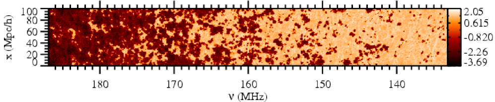
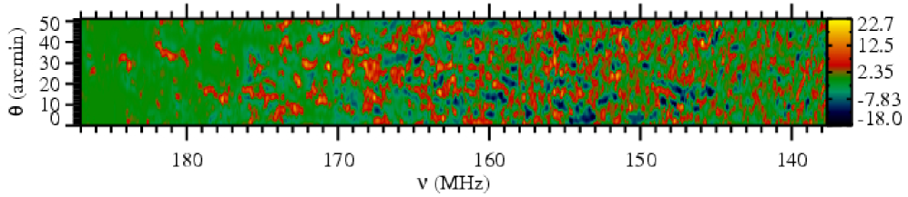
Figure 1: Position-redshift slices from the f250C simulation. These slices illustrate the large-scale geometry of reionization and the significant local variations in reionization history as seen at redshifted 21-cm line. Observationally they correspond to slices through an image-frequency volume. The top image shows the decimal log of the differential brightness temperature at the full grid resolution, while the bottom image shows the same $T_{b}$ data, but in linear scale and smoothed with a compensated Gaussian beam of 3’ and (tophat) bandwidth of 0.2 MHz, roughly corresponding to the expected parameters for LOFAR. The spatial scale is given in comoving units (top) or (approximate) angle on the sky in arcminutes (bottom).

3 21-cm emission

The differential brightness temperature with respect to the CMB of the redshifted 21-cm emission is determined by the density of neutral hydrogen, $\rho_{\rm HI}$, and its spin temperature, $T_{\rm S}$. It is given by

$$\delta T_{b} = \frac{T_{\rm S}-T_{\rm CMB}}{1+z}(1-e^{-\tau})$$

$$\approx \frac{T_{\rm S}-T_{\rm CMB}}{1+z}\frac{3\lambda_{0}^{3}A_{10}T_{*}n_{HI}(z)}{32\pi T_{S}H(z)}$$

$$= {28.5\,\rm mK}\left(\frac{1+z}{10}\right)^{1/2}(1+\delta)\left(\frac{\Omega_{b}}{0.042}\frac{h}{0.73}\right)\left(\frac{0.24}{\Omega_{m}}\right)^{1/2}$$

(Field 1959), where $z$ is the redshift, $T_{\rm CMB}$ is the temperature of the CMB radiation at that redshift, $\tau$ is the corresponding 21-cm optical depth, $\lambda_{0}=21.16$ cm is the rest-frame wavelength of the line, $A_{10}=2.85\times 10^{-15}\,\rm s^{-1}$ is the Einstein A-coefficient, $T_{*}=0.068$ K corresponds to the energy difference between the two levels, $1+\delta={n_{\rm HI}}/{\langle n_{H}\rangle}$ is the mean number density of neutral hydrogen in units of the mean number density of hydrogen at redshift $z$,

$$\langle n_{H}\rangle(z) = \frac{\Omega_{b}\rho_{\rm crit,0}}{\mu_{H}m_{p}}(1+z)^{3}$$ (2)

$$= 1.909\times 10^{-7}\rm cm^{-3}\left(\frac{\Omega_{b}}{0.042}\right)(1+z)^{3},$$

with $\mu_{H}=1.32$ the corresponding mean molecular weight (assuming 32% He abundance by mass), and $H(z)$ is the redshift-dependent Hubble constant,

$$H(z) = H_{0}[\Omega_{\rm m}(1+z)^{3}+\Omega_{\rm k}(1+z)^{2}+\Omega_{\Lambda}]^{1/2}$$ (3)

$$= H_{0}E(z)\approx H_{0}\Omega_{\rm m}^{1/2}(1+z)^{3/2},$$

where $H_{0}$ is its value at present, and the last approximation is valid for $z\gg 1$. Throughout this work we assume that all of the neutral IGM gas is Ly-$\alpha$-pumped and sufficiently hot (due to e.g. a small amount of X-ray heating) above the CMB temperature and is thus seen in emission. These assumptions are generally well-justified, except possibly at the earliest times (see e.g. Furlanetto et al. 2006, and references therein).

3.1 The progress of reionization: global view

The images in Figure 1 show the progress of reionization as seen at 21-cm emission vs. the observed frequency for run f250. The technique we used to produce them was described in detail in Mellema et al. (2006b) and is similar to the standard method for making light-cone images. In short, it involves continuous interpolation between the single-redshift numerical outputs in frequency/redshift space. The slices are cut at an oblique angle so as to avoid repetition of the same structures along the same line-of-sight. Redshift-space distortions due to peculiar bulk velocities are included. The top image shows the decimal logarithm of the differential brightness temperature at the full resolution of our simulation data, approximately 0.25 arcmin in angle and 30 kHz in frequency. The ionization starts from the highest density peaks, which is where the very first galaxies form. These high peaks are strongly clustered at high redshifts, which results in a quick local percolation of the ionized regions. As a result, by $z\sim 9$ ($\nu_{\rm obs}\sim 140$ MHz) already a few fairly large ionized regions form, each of size $\sim 10$ Mpc. These continue to grow and overlap until there is only one topologically-connected H II region in our computational volume, which for this particular simulation occurs at $z\sim 7$ ($\nu_{\rm obs}\sim 180$ MHz). However, even at this time quite large, tens of Mpc across, neutral regions still remain. They are gradually ionized as time goes on, but some of them persist until the very end of our simulation. The uncertaities in the reionization parameters (e.g. source efficiencies, gas clumping) result in moderate variations in the typical sizes of the ionized and neutral regions, but do not change the basic characteristics of the reionization process.

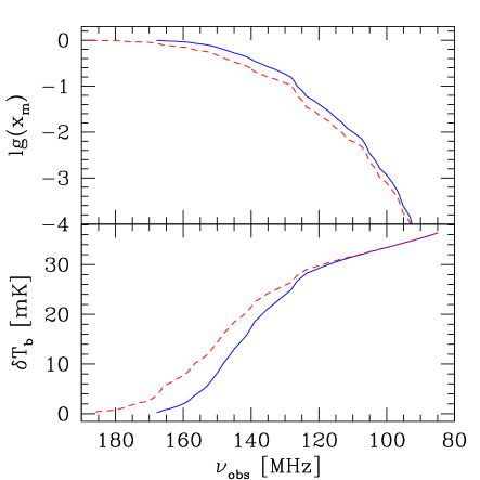
Figure 2: Evolution of the mean mass-weighted ionized fraction, $x_{m}$, (top), mean flux in $\mu$ Jy (assuming a circular beam with an angular diameter of 10’) (middle) and the mean differential brightness temperature, $\delta T_{b}$, in mK vs. observed frequency for simulations f250 (solid, blue), and f250C (short-dashed, red).

The bottom image in Figure 1 shows the same data as the top, but as would be seen by a radio interferometer array assuming perfect foreground removal. To obtain it we smoothed the data with a compensated Gaussian beam with FWHM of 3’ and bandwidth of 0.2 MHz, similar to the expected parameters for the LOFAR array. Unless otherwise stated, throughout this paper we use a compensated Gaussian beam. We recognise that a compensated Gaussian is not perfect match to the actual interferometer beam, however it captures its essential properties. In particular, it has zero mean, and negative troughs at the side of the central peak (see e.g. Mellema et al. 2006b). As a result, ionized regions show as negative differential brightness temperature regions if they are surrounded by neutral volumes. If an ionized (or a neutral) region is much larger than the smoothing scale, the resulting signal would be close to zero. A direct comparison between the two images shows that all the main structures clearly remain also in the smoothed image, indicating that LOFAR and other similar interferometers would have sufficient resolution to determine the large-scale reionization morphology to a reasonable accuracy throughout most of the reionization history. However, at the earliest stages of reionization some of the existing H II regions are barely seen, or not at all, since the beam smoothing either merges them with other nearby ionized regions, or simply smoothes them away. This is a consequence of the small sizes of these early H II regions, which puts the majority of them below the beam resolution. At frequencies higher than $\sim 140$ MHz the ionized bubbles become large enough to be above the smoothing scale and thus all major structures become visible. Higher ionizing source efficiencies and/or lower gas clumping would yield somewhat larger H II regions, thus they would become visible slightly earlier. We also note that the Cosmic Dark Ages and the early stages of reionization might be still observable through other sources of 21-cm fluctuations which we do not consider here. These include e.g. the 21-cm emission and absorption by cosmological minihaloes (Iliev et al. 2002; Furlanetto & Loeb 2002; Iliev et al. 2003), by shock-heated IGM (Furlanetto & Loeb 2004; Shapiro et al. 2006), or due to inhomogeneous early backgrounds in Ly-$\alpha$ (Barkana & Loeb 2005; Chuzhoy et al. 2006) or X-rays (Pritchard & Furlanetto 2006). We note that there are bright and potentially observable features even for $\nu_{\rm obs}>180$ MHz. This is important for the planned observations since at such high frequencies both the foregrounds and the Radio Frequency Interference (RFI) are substantially lower, while at the same time the array sensitivities improve. We discuss these issues in more detail in § 3.3.

In Figure 2 we show the evolution of the mean (i.e. averaged over a large volume) mass-weighted ionization fraction, $x_{m}$, and the mean differential brightness temperature as seen at the observer, $\overline{\delta T_{b}}(\nu_{\rm obs})$. As the universe steadily becomes ever more ionized, the mean 21-cm differential brightness temperature naturally decreases. However, the signal persists at a non-trivial level (a few mK or more) until quite late,up to frequencies of 150-170 MHz. Similarly to our previous results which used the WMAP1 parameters, the “global step” from mostly-neutral to mostly-ionized medium (Shaver et al. 1999) turns out to be rather gradual, with the signal decreasing by $\sim 20$ mK over 20-30 MHz (and somewhat more gradual for case f250C than for f250). The differential brightness temperature scales with the reionization redshift as $\delta T_{b}\propto(1+z)^{1/2}$. Thus, a delay of reionization from WMAP1 to WMAP3 model by 1.3 in redshift corresponds to an expected $\delta T_{b}$ decrease by a factor of 1.14, roughly as found in our simulations.

Analytical models of the globally-averaged 21-cm signal (Sethi 2005; Furlanetto 2006, e.g.) predict evolutions which are in rough agreement with ones we find. The models considered in Sethi (2005) yielded a somewhat faster evolution of the global signal, while the wider range of models presented in Furlanetto (2006) included cases of both faster and of more gradual evolution, depending on the details of the evolution of the Ly-$\alpha$ and X-ray backgrounds.

3.2 The statistical measures

An alternative approach to take would be a statistical one, through detection of the fluctuations of the emission around its mean value (see Scott & Rees 1990; Madau et al. 1997; Iliev et al. 2002; Zaldarriaga et al. 2004; Morales & Hewitt 2004; Mellema et al. 2006b; Furlanetto et al. 2006, and references therein). These fluctuations are due to a combination of the reionization patchiness and the variations of the underlying density field. In Figure 3 we show the rms of the 21-cm emission fluctuations derived from our simulations. The top panel shows the evolution of the differential brightness temperature rms, $\delta T_{\rm b,rms}$, for three choices for the beam size (in arcmin; using compensated Gaussian beam) and the bandwidth (in MHz), from top to bottom, $(\Delta\theta_{\rm beam},\Delta\nu_{\rm bw})=(0.1,1)$ (roughly as expected for the SKA compact core), $(0.2,3)$ (LOFAR) and $(0.4,6)$ (GMRT, MWA). The middle panel shows the evolution of the corresponding fluxes, given by

$$\delta F(\nu_{\rm obs})=\frac{2\nu_{\rm rec}^{2}}{c^{2}}k_{B}\delta T_{b}(\nu_{\rm obs})\Delta\Omega,$$ (4)

where $\Delta\Omega=\pi(\theta/2)^{2}$ is the 3D angle subtended by the beam for a circular beam with FWHM of $\theta_{\rm beam}$. On the bottom panel we show the 21-cm signal as a fraction of the dominant foreground, the Galactic synchrotron emission. For the larger beams/bandwidths the $\delta T_{b,rms}$ peak is at $z\sim 8.8$ ($\nu_{\rm obs}\sim 145$ MHz) for f250 and at $z\sim 8.3$ ($\nu_{\rm obs}\sim 152-153$ MHz to for f250C, close to the time at which 50% of the mass is ionized, as was the case also for our WMAP1 results (Mellema et al. 2006b). However, for the higher resolution, corresponding to a $1^{\prime}$ beam, the peak of the fluctuations moves to noticeably earlier times/lower frequencies, to $\sim 137$ MHz ($x_{m}=0.26$) for f250 and to $\sim 143$ MHz ($x_{m}=0.26$) for f250C. This high-resolution case differs from the rest because the scales probed by such a small beam/bandwidth combination are generally below the characteristic bubble size. The exception is at early times, when ionized bubbles are still small on average, and thus match better the smaller beam-size, which is reflected in the fluctuation peak moving to earlier times.

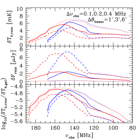
Figure 3: (a)(top) rms fluctuations of the differential brightness temperature, $\delta T_{\rm b,rms}\equiv\langle\delta T_{b}^{2}\rangle^{1/2}$ vs. observed frequency, $\nu_{\rm obs}$ for f250 (blue) and f250C (red) for beam sizes and bandwidths $\Delta\theta_{\rm beam},\Delta\nu_{\rm bw})=$(1’,0.1 MHz) (dotted), (3’,0.2 MHz) (solid) and (6’,0.4 MHz) (dashed); (b)(middle) Fluxes in $\mu Jy$ corresponding to the differential brightness temperature fluctuations in (a), same notation as in (a); and (c)(bottom) Ratio of $\delta T_{\rm b,rms}$ to the mean Galactic synchrotron foreground, assumed to be $\delta T_{\rm b,gal}=300\,\rm K(\nu/150\,MHz)^{-2.6}$, same notation as in (a).

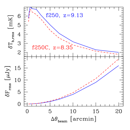
Figure 4: (a)(top) rms fluctuations of the differential brightness temperature, $\delta T_{\rm b,rms}\equiv\langle\delta T_{b}^{2}\rangle^{1/2}$ vs. beam-size, $\delta\theta_{\rm beam}$ for f250 (solid, blue) and f250C (short-dashed, red) at redshifts close to the maximum of the fluctuations, as indicated. The bandwidth is changed in proportion to the beamsize. (b)(bottom) Flux fluctuations corresponding to the differential brightness temperature fluctuations in (a), same notation as in (a).

Figure 5: The variance, $\Delta$ of the 3D power spectra of the neutral gas density $\Delta_{\rho,HI}$ (dotted), and the total density $\Delta_{\rho}$ (solid), normalized to the total, for simulations f250 (left) and f250C (right). The redshifts are chosen as follows (in decreasing numerical order): early times ($z=12$; $\overline{T_{b}}=31.8$ mK for f250, $\overline{T_{b}}=33.2$ mK for f250C), the redshift at which $\delta T_{\rm b,rms}$ peaks ($z=8.8$, $\overline{T_{b}}=13.1$ mK for f250, $z=8.3$, $\overline{T_{b}}=11.8$ mK for f250C), the redshift at which $\delta F_{\rm rms}$ peaks ($z=8.5$, $\overline{T_{b}}=8.9$ mK for f250; $z=7.9$, $\overline{T_{b}}=8.2$ mK for f250C), and the redshift of overlap ($\overline{T_{b}}=0.3$ mK for f250; $\overline{T_{b}}=0.2$ mK for f250C).

We note that the flux fluctuations peak somewhat later than the corresponding temperature fluctuations. The position of the peak flux in redshift/frequency space is largely independent of the resolution employed, and is at $\sim 148-150$ MHz for f250 and at $\sim 155-157$ MHz for f250C. As the beam-size and bandwidth increase from 1’ to 3’ and then to 6’, the temperature fluctuations decrease, albeit only by a modest amount. For example, the peak fluctuations for $(\Delta\theta_{\rm beam},\Delta\nu_{\rm bw})=$(6’,0.4 MHz) are only a factor of $\sim 2$ lower (4 mK vs. 8 mK), while the corresponding flux increases by over an order of magnitude, indicating that it would be optimal to observe at relatively large scales, where we maximize the sensitivity without sacrificing much of the signal.

Higher source efficiency and lower gas clumping would result in the bubbles at the same redshift being a bit larger in typical size. This would move the peak position to a bit lower frequency. It would also make it slightly higher for the larger beam sizes since larger bubble sizes at the half-ionized point would match these beamsizes better.

The 21-cm temperature fluctuations as fraction of the dominant foreground, the Galactic synchrotron emission (bottom panel) peak even later than the flux fluctuations. This is due to the broad peak of the 21-cm emission and the steep decline of this foreground at higher frequencies, which combine to push the peak to later times/higher frequencies, at $\nu_{\rm obs}$ up to 160-165 MHz. The signal is strongly dominated by the foregrounds at all times, but up to an order of magnitude could be gained for observations aimed close to the peak ratio, as opposed to earlier or later times. Furthermore, observing with an interferometer removes significant part of the foregrounds, due to the differential nature of the measurements. This eliminates the uniform component of the foregrounds, leaving only its fluctuations, at the level of 1-10% of the total.

In Figure 4 we plot the differential brightness temperature fluctuations and the corresponding fluxes vs. the instrument smoothing, as given by the beam size, with the bandwidth changed in proportion to the beam size. At small scales (below the typical ionized bubble size, a few arcmin or less) the temperature fluctuations are fairly large ($>6$ mK) and dominated by Poisson fluctuations (e.g. a cell is either ionized or else is neutral). However, the corresponding flux is tiny, below 1 $\mu Jy$. Around the typical bubble scale ($\sim 5-10^{\prime}$) the fluctuations are slightly lower, at $\sim 3-4$ mK, but the flux grows strongly, as $\delta\theta_{\rm beam}^{2}$ and reaches $\sim 5\mu Jy$ at $\delta\theta_{\rm beam}=10^{\prime}$. At even larger angles/bandwidths the ionization fluctuations gradually start contributing ever less to the total and in the large-scale limit the temperature fluctuations just follow the underlying large-scale density fluctuations (multiplied by the mean differential brightness temperature). The flux curve should gradually flatten and at some point there would be little to be gained by a further increase of the observed sky patch since the gain in angle is canceled by the decrease of the temperature fluctuations. Thus, again there is a trade-off between the signal level and the array sensitivity. The optimal scale for observations will depend on the best sensitivity which could be achieved by a particular radio array. For compact arrays the optimal beam size is around 10-20’, but could be lower than that for sensitive arrays with large collecting area like SKA.

Finally, in Figure 5 we show the three-dimensional power spectra of the density and the neutral gas density fluctuations (to which the 21-cm signal is directly proportional) at several illustrative redshifts. Initially, the neutral density power largely tracks the one of the density field, since most of the gas is still neutral. At intermediate and late times the ionization fraction inhomogeneities introduce a peak around the characteristic scale of the ionized patches (which is $k\sim 1\,h\,Mpc^{-1}$ for f250C, and slightly lower for f250). Around the time when the fluctuations reach their peak the patchiness boosts the power on large scales by factor of $\sim 2$ (1.5) for f250 (f250C) compared to the density power spectrum. The signal largely disappears around the time of overlap, since little neutral hydrogen remains, but the power spectra still show the characteristic peak, at approximately the same scales.

Some of the most visible redshifted 21-cm features would be the points of maximum departure of the signal from the mean. The magnitude of the signal is dependent on the level of smoothing and could evolve with redshift. The maxima/minima are roughly independent of redshift, within factor of $\sim 2$, but there are also some interesting and nontrivial features. For the case of no smoothing (i.e. at full grid resolution, $\sim 0.25^{\prime}$, 30 kHz) the maximum amplitude is quite high, at $\sim 100-200$ mK. Naturally, the beam smoothing decreases the amplitude, to $\sim 20-30$ mK for $(\Delta\theta_{\rm beam},\Delta\nu_{bw})=(1^{\prime},0.1\,\rm MHz)$, 10-20 mK for $(\Delta\theta_{\rm beam},\Delta\nu_{bw})=(3^{\prime},0.2\,\rm MHz)$ and to 8-20 mK for $(\Delta\theta_{\rm beam},\Delta\nu_{bw})=(6^{\prime},0.4\,\rm MHz)$. The introduction of sub-grid clumping (f250 vs. f250C) results in only minor variations here. The absolute value of the minimum is similar to the one for the maximum in all cases, but the two still show some differences. For the larger beams/bandwidths the maxima peak around the time of 50% ionization by mass, while the absolute values of the minima peak noticeably earlier. This is readily understood based on the evolution of the typical ionized and neutral region sizes and the properties of the compensated Gaussian beam. Early-on the ionized regions are small and isolated, surrounded by large neutral patches, which yields deep negative minima at the positions of the ionized bubbles. At late times the H II regions grow large and the beam-smoothed signal inside them is close to zero. The positive maxima, on the other hand, are due to the densest neutral regions and are sampled by the central maximum of the beam, and thus reach their peak later.

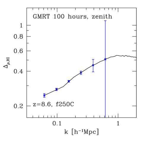
Figure 6: Observability of the 21-cm signal: the 3D power spectrum of the neutral hydrogen density, $\Delta_{\rho,HI}$, at redshift $z=8.59$ ($\overline{T_{b}}=16.3$ mK) with the forecast error bars for 100 hours observation with GMRT vs. wavenumber $k$. We assumed 15 MHz observing bandwidth (the full instantaneous bandwidth of GMRT), $T_{\rm sys}=480$ K and $T_{S}\gg T_{\rm CMB}$. The array configuration is assumed pointed to the zenith, but the sensitivity is only weakly dependent on the pointing.

The statistics of these emission peaks is also of considerable interest since it shows how common such features are and thus what patch of sky one needs to study for a detection. PDFs of the 21-cm emission are similar to the ones we previously found for the WMAP1 cosmology (Iliev et al. 2006b). They are considerably non-Gaussian, especially at late times and smaller smoothing scales. In particular, for smoothing scales of $\sim 5-10$ Mpc there is an over-abundance of the brightest regions by up to an order of magnitude compared to the a Gaussian with the same mean and rms. At large scales ($\lower 2.15277pt\hbox{$\;\buildrel>\over{\sim}\;$}20\,h^{-1}$ Mpc) and late times the PDFs become very close to Gaussian.

3.3 Observability: redshifted 21-cm

There are several current or upcoming experiments which aim to detect the redshifted 21-cm signatures of reionization, including LOFAR, MWA, GMRT, PAST/21CMA and SKA. Not all details of the design and the instruments are yet known, particularly for SKA for which even the basic concept is not yet finalized. The only arrays currently in operation are GMRT and PAST/21CMA. Among these interferometers, GMRT and LOFAR have the largest collecting area, at $\sim 50,000\,\rm m^{2}$ for GMRT and (effective) $\sim 10^{5}\,\rm m^{2}$ for LOFAR at 110-200 MHz, and thus in principle they have the best sensitivity before the commissioning of SKA. However, the same two arrays also have significant interference problems to overcome from terrestrial sources of confusion. As an example, in Figure 6 we show our predicted 21-cm signal at $z=8.6$ (case f250C) along with the anticipated GMRT sensitivity to the 3D power spectrum for 100 hours of integration. The sensitivity is calculated using the baseline distribution as seen from zenith, angle averaged, and optimally weighted. Radially, the velocity resolution has been assumed higher than any scale of interest, which is achievable with the recently-developed new software correlator. The error on modes are anisotropic for radial versus azimuth and the errors are combined by weighting each mode by its sum of noise and signal variance. We assumed 15 MHz observing bandwidth (the full instantaneous bandwidth of the GMRT correlator, the frequency resolution is much better, of order kHz) and $T_{\rm sys}=480$ K. The errors calculation assumes Gaussian noise and Gaussian source statistics, and a 7 square degree field of view. The two small-$k$ bins would probably not be observable due to foreground removal. We note that previous literature concentrated on two dimensional noise models for experiments, and for reference in Figure 7 we show the expected band-averaged azimuthal GMRT thermal noise power spectrum for bandwidth of 15 MHz, 100 hours of integration, and a single pointing. Noise is estimated using the standard radio telescope noise estimation formulae:

$$T_{\rm map}=\frac{T_{\rm sys}}{B\sqrt{\delta\nu\delta t}},$$ (5)

where $B$ is the angular-scale dependent effective beam response obtained by summing over all the baselines assuming the telescope is pointed at the zenith. It changes only slightly when looking elsewhere. The beamnoise then is simply the Fourier transform of $T_{\rm map}$. The other two arrays, PAST/21CMA ($\sim 10^{4}\,\rm m^{2}$ effective area) and MWA ($\sim 7000\,\rm m^{2}$) are significantly smaller than either LOFAR or GMRT, but are also more compact and would be constructed in areas with very low interference. Thus, they could also be quite competitive, at least in terms of detecting 21-cm fluctuations at very large scales, because of their low spatial resolution.

Figure 7: Observability of the 21-cm signal: forecast angular power spectrum of thermal noise of GMRT for bandwidth of 15 MHz, 100 hours of integration, one single pointing.

Our results indicate that the 21-cm fluctuations in WMAP3 cosmology peak around $\nu_{\rm obs}=130-170$ MHz (compared to 90-120 MHz for WMAP1 models), depending on the resolution and the detailed reionization parameters (ionizing source efficiencies and gas clumping). The corresponding 21-cm flux fluctuations, and the 21-cm temperature fluctuations as fraction of the foregrounds peak at even higher frequencies. These properties significantly facilitate the signal detection as compared to the WMAP1 cases, since at higher frequencies the detector sensitivities are dramatically better, while at the same time the foregrounds are lower, by roughly factor of $\sim(120/170)^{2.6}=2.5$. The peak value of the differential brightness temperature fluctuations is $\sim 4-8$ mK, decreasing modestly with increasing beam and bandwidth. The corresponding fluxes are much more strongly dependent on the scale of observations, ranging from $<1\mu\,\rm Jy$ for 1’ beam and 0.1 MHz bandwidth to $\sim 8\mu\,\rm Jy$ for 6’ beam and 0.4 MHz bandwidth. This clearly argues for relatively large beams, of at least a few arcmin, and for maximum collecting area concentrated in the compact core, in order to improve the sensitivity while not losing a significant fraction of the signal. For example, the expected sensitivity of LOFAR for 1 hour of integration time is $\sim 0.6\,\rm mJy$ for bandwidth of 1 MHz (and somewhat worse for the virtual core only), while its resolution is 3.5”-6” for the whole array and 3’-5’ for the core (numbers are frequency-dependent). Thus, only the virtual core would be useful for EOR observations (although the extended part would be important for e.g. better foreground subtraction). Upwards of $100$ hours of integration time would be needed for detection, less if more antennae are placed in the virtual core.

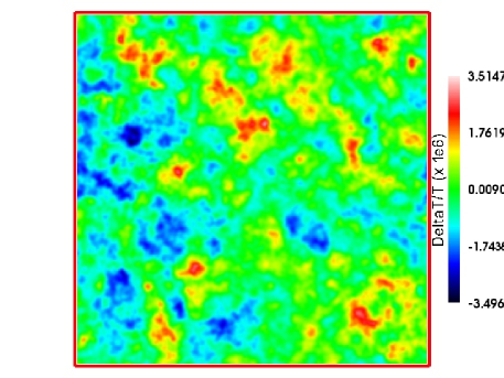
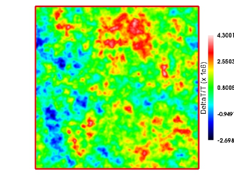
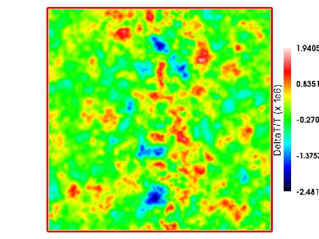
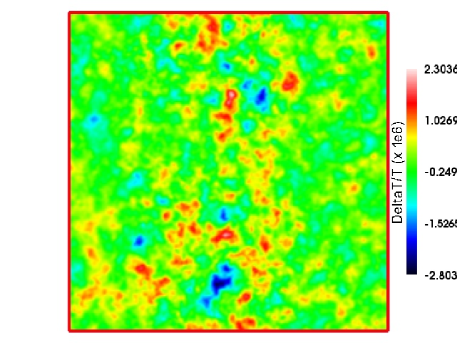
Figure 8: kSZ temperature fluctuation maps from simulations: f250 with large-scale velocities (top left), f250C with large-scale velocities (top right), f250 (bottom left), and f250C (bottom right). (Images produced using the Ifrit visualization package of N. Gnedin).

The importance of aiming at the appropriate frequencies and length scales cannot be overstated. As we have shown, around the peak of the fluctuations the signal as fraction of the dominant foreground is up to an order of magnitude larger than it is off the peak. Utilizing an appropriate beam, i.e. one which is well-matched to the scale of the expected fluctuations and corresponding to sufficiently large flux level, given the available sensitivity, is also extremely important. Our results indicate that the best beam sizes are of at least a few arcminutes, and possibly much larger, of order 5-10’ or more. Larger ionizing source efficiencies or lower gas clumping would change the height and position of the peak fluctuations slightly, but our main conclusions in terms of the best observation strategies and frequency band to observe would remain valid. Once more observation data becomes available the reionization scenarios presented here can be refined to give us better constraints on the ionizing sources.

Another observational strategy, and one of the first to be proposed (Shaver et al. 1999) is to aim to detect the “global step” over the whole sky which reflects the transition from the fully-neutral universe before reionization to the fully-ionized one after (see Shaver et al. 1999, for more detailed discussion of the various observational issues). Since this is a global, all-sky signal it imposes essentially no requirements in terms of resolution. The sensitivity requirements are also relatively modest, since the flux corresponding to such a large area on the sky is very large. The main difficulty is the foreground subtraction. The global step we find is relatively gradual, $\sim 20$ mK over $\sim 20$ MHz. This would still be readily detectable in absence of foregrounds. How well the foregrounds could be subtracted would depend strongly on their properties, and in particular how fast and by how much the local slope of the power law describing it changes. If the foregrounds are well-fit by a single power law over the relevant frequencies, then there is a good chance to detect the global transition signal, see Shaver et al. (1999) for more detailed discussion.

The brightness temperature behaviour we find suggests that the best frequency range to aim for could be $\sim 120-150$ MHz, since there the signal decrement is largest. A slightly higher overall normalization of the primordial density fluctuation power spectrum, as suggested by combining all the available data sets would shift the best frequency range to slightly lower frequencies, but ones which are still above the FM range ($\nu>110$ MHz). Only a fairly high normalization, $\sigma_{8}\sim 0.9$ and no power spectrum tilt (as given by WMAP1) would shift the global step into the FM range ($90\,\rm MHz<\nu<110$ MHz). However, such a high normalization is largely excluded by the best current fits to the cosmological parameters.

We also note that albeit at first sight it appears that modifying the background cosmology is degenerate with assuming different source efficiencies, in fact the two options are not equivalent. A different background cosmology changes the timing of reionization to earlier or later, i.e. is simply a shift in redshift due to the delay or acceleration of structure formation, as previously pointed out in Alvarez et al. (2006). On the other hand, changing the source efficiencies has a somewhat different effect - either extending or shortening the duration of reionization - for given power spectrum parameters the sources form at the same time and same numbers, the different efficiencies just mean that their effect is stronger or weaker, thereby extending or shortening reionization, as we have discussed in Mellema et al. (2006b). While this is a somewhat subtle distinction, it does yield different shapes of $dT_{b}(z)$, so the two cases can in principle be distinguished and are thus not equivalent.

An important reionization signature to look for is the one due to individual, rare, bright features. The magnitude of such features depends on the scale observed, ranging from $\sim 0.1$ K for high resolution (0.25’, 30 kHz), to few tens of mK for beams of size a few arcminutes. The peak magnitude is only weakly dependent on redshift, with the peak value within a factor of two of the typical values. The redshift/frequency at which the peak is reached is beamsize-dependent, moving to higher frequencies for larger beams. Taking also into account the much larger fluxes corresponding to larger beams, this again clearly argues for utilizing relatively large beams (5’-10’ or more) and aiming at the high frequencies ($\sim 130-160$ MHz) for such observations. The statistics of such rare, bright peaks are also favourable at late times, we find that at $\sim 3^{\prime}-5^{\prime}$ scales there are up to an order of magnitude more such peaks than a Gaussian statistics would predict.

4 kSZ effect from patchy reionization

Next, we turn our attention to the second main reionization observable, the small-scale secondary CMB anisotropies generated through the kinetic Sunyaev-Zel’dovich (kSZ) effect (Zeldovich & Sunyaev 1969; Sunyaev & Zeldovich 1980; Ostriker & Vishniac 1986; Vishniac 1987; Jaffe & Kamionkowski 1998; Gruzinov & Hu 1998; Hu 2000; Gnedin & Jaffe 2001; Springel et al. 2001; Ma & Fry 2002; Santos et al. 2003; Zhang et al. 2004; Zahn et al. 2005; McQuinn et al. 2005; Salvaterra et al. 2005; Iliev et al. 2007b). The kSZ effect results from Thomson scattering of the CMB photons onto electrons moving with a bulk velocity $v$. Along a line-of-sight (LOS) defined by a unit vector ${\bf n}$ the kSZ temperature anisotropies are given by:

$$\frac{\Delta T}{T_{\rm CMB}}=\int d\eta e^{-\tau_{\rm es}(\eta)}an_{e}\sigma_{T}\frac{{\bf n}\cdot{\bf v}}{c},$$ (6)

where $\eta=\int_{0}^{t}dt^{\prime}/a(t^{\prime})$ is the conformal time, $a$ is the scale factor, $\sigma_{T}=6.65\times 10^{-25}\,\rm cm^{-2}$ is the Thomson scattering cross-section, and $\tau_{\rm es}$ is the corresponding optical depth. Since our simulation volume is not large enough to follow the complete photon light path from high redshift to the end of reionization, we have to combine several simulations volumes. In order to avoid artificial effects from the box repetition (in particular having the same structures repeating over and over along the photon path) we randomly shift the simulation box along both directions perpendicular to the ray direction and also alternate the x-, y- and z-directions of the box. We have presented our detailed methodology along with our predictions for the kSZ reionization signal based on the WMAP1 cosmology in Iliev et al. (2007b). Some of the power from the largest-scale velocity field perturbations is missing from the simulation data, due to our finite box size. We compensate for that missing power by adding it in a statistical way, again as discussed in detail in Iliev et al. (2007b).

4.1 The kSZ signal

The resulting kSZ maps are shown in Figure 8. The full scale of the maps corresponds to our full simulation box size ($100\,h^{-1}$ Mpc, or $\sim 50^{\prime}$) and the pixel resolution corresponds to the simulation cell size ($100\,h^{-1}/203\,\rm Mpc\approx 0.5\,h^{-1}Mpc$, or $\sim 0.25^{\prime}$). At a few arcminute scale there are a number of fluctuations larger than 5 $\mu$K with both positive and negative sign. The f250 and f250C runs yield largely similar level of fluctuations, slightly larger ones in the latter case. The typical scale of the kSZ temperature fluctuations in run f250 is also a bit larger than the scale for f250C, reflecting the larger, on average, sizes of the ionized regions in the former case compared to the latter. Introducing the correction for the missing large-scale velocity power increases the fluctuation range by about 50% and introduces some large-scale coherent motions.

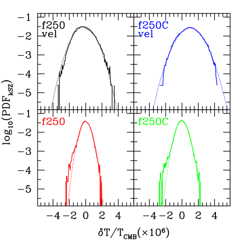
Figure 9: PDF distribution of $\delta T_{\rm kSZ}/T_{\rm CMB}$ (solid) vs. Gaussian distribution with the same mean and width (dotted) with (top panels) and without (bottom panels) correction for the large-scale velocity power missing from the computational box for our simulations, as labelled.

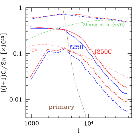
Figure 10: Sky power spectra of $\delta T_{\rm kSZ}/T_{\rm CMB}$ fluctuations resulting from our simulations: f250 (blue), and f250C (red). Solid (dashed) lines show the results with (without) the correction for the large-scale velocity power missing from the box. compared to the after-reionization kSZ signals (assuming overlap at $z_{\rm ov}=8$): linear Ostriker-Vishniac effect, labelled ’OV’ (long-dashed, pink), and a fully-nonlinear model matched to high-resolution hydrodynamic simulations of Zhang et al. (2004), labelled ‘Zhang et al’ (short-dashed, dark green). We also show the total (patchy reionization + Zhang et al. post-reionization) signals (dot-dashed; top lines) and the primary CMB anisotropy signal (dotted, brown).

In Figure 9 we show the PDF of these kSZ maps. The full range of the temperature fluctuations at pixel level is $\pm 20\,\mu$K ($\pm 13\,\mu$K) with (without) the large-scale velocity corrections. The rms fluctuations of $\Delta T/T_{\rm CMB}$ for run f250 are $4.835\times 10^{-7}$ ($8.968\times 10^{-7}$) without (with) large-scale velocities, while for run f250C the numbers are $5.094\times 10^{-7}$ ($1.020\times 10^{-6}$) without (with) large-scale velocities. Both the range and the rms of the kSZ fluctuations are lower than the corresponding quantities we derived from the WMAP1 reionization scenarios by factor of $\sim 2$, thus the PDF distributions are correspondingly less wide. In both WMAP3 cases there are some mild departures from Gaussianity at the bright end. Adding the correction for the large-scale velocities yields wider (by factor of $\sim 2$) and, interestingly, much more Gaussian PDF distributions.

Since the kSZ effect is a product of electron density and velocity, a naive expectation is that the kSZ angular power spectrum would scale as $\sigma_{8}^{2}$ for the density and $\sigma_{v}^{2}$ for the velocity, $\sigma_{8}^{4}$ in total. The actual ratio we find is $\sigma_{8}^{3.94}$ for reionization scenario f250C and $\sigma_{8}^{3.83}$ for f250. However since $8\,h^{-1}$Mpc is well above the scales relevant to reionization, thus in the presence of tilt a more appropriate scaling would be a bandpower at dwarf galaxy scales, $\sigma_{0.1}^{2}$, introduced in § 2, rather than at galaxy cluster scales, $\sigma_{8}^{2}$. We find the kSZ power scales as one power less, $\propto\sigma_{0.1}^{2.74}$ for f250C and $\propto\sigma_{0.1}^{2.82}$ for f250. This scaling also holds true for the minihalo bandpower, $\sigma_{0.01}^{2}$. Thus it becomes insensitive to the exact length scale once we are in the relevant part of the power spectrum. As we mentioned in § 1, the values of $\sigma_{0.01}$ and $\sigma_{0.1}$ scaled to include the growth inhibition between high redshift and redshift zero, $(a/D)\approx\Omega_{m}^{0.23}$, 0.74 and 0.76 for the WMAP3 and WMAP1 cases, provide a good indication when the hierarchy spanning the collapse of first the minihaloes then the dwarfs developed.

The output from radio telescopes is sky power spectra, shown in Figure 10. The kSZ signal from patchy reionization dominates the primary anisotropy at small scales, for $\ell>4000$. The magnitude of the signal is $[\ell(\ell+1)C_{\ell}/2\pi]\sim 10^{-13}$, or $\Delta T\sim 1\,\mu$K. The presence of sub-grid gas clumping boosts the power by $\sim 50\%$ for $\ell>4000$, but has little effect on the power spectrum shape. Adding the correction for the missing velocity power at large-scales boosts the signal power by additional factor of 2-3 in the interesting range of scales ($\ell>4000$). At larger scales the boost is larger, by up to an order of magnitude, but at those scales the kSZ temperature anisotropy is strongly dominated by the primary CMB. Compared to the predicted post-reionization anisotropy signals, the kSZ from patchy reionization is larger than the linear Ostriker-Vishniac signal (OV) for $\ell<20,000$ and slightly lower than, but similar to the full nonlinear post-reionization effect prediction by Zhang et al. (2004) (which we rescaled to the current WMAP3 cosmology using the scaling $C_{\ell}\propto\sigma_{8}^{5}$). The total, patchy reionization and post-reionization (based on Zhang et al. (2004)) signals are also shown at the top of the figure. The total power spectrum retains the peak at $\ell\sim 3000-4000$ imprinted by the patchy reionization component, although the signal decrease at small scales is not as pronounced, since the decrease is partially compensated for by the continuing weak rise of the post-reionization component of the signal. The two reionization scenarios (red and blue top curves) would be very difficult to distinguish based solely on the total signal, but this might be possible to do if the post-reionization component is known sufficiently well and is subtracted to a good precision (see also the next section). A slightly higher power spectrum normalization, as suggested by recent cosmological parameter estimates, will moderately increase the signal as indicated by the above scalings. However, the strongly-peaked shape of the signal will persist, since it is reflecting the characteristic scales of the reionization process. Higher source efficiencies would shift the peak some towards larger scales, reflecting the larger typical size of the bubbles (due to the combination of the higher source efficiencies and the stronger source clustering at higher redshift) in this case.

4.2 Observability: kSZ from patchy reionization

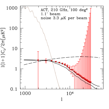
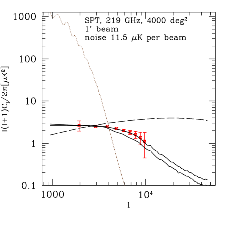
Figure 11: Observability of the kSZ: the sky power spectrum of the reionization signal (black, solid; simulations f250 and f250C) with the forecast error bars for ACT (left) and SPT (right) vs. $\ell$. The primary CMB anisotropy (dotted) and the post-reionization kSZ signal (dashed) are also shown and are added to the noise error bars for the reionization signal. Cosmic variance from tSZ would increase the error bars, but here we are assuming that the tSZ component has been completely separated, by virtue of its characteristic spectral shape.

The Atacama Cosmology Telescope (Fowler 2004; Kosowsky & the ACT Collaboration 2006), currently entering into operation, will observe at three frequency channels, at 147, 215 and 279 GHz, targeting clear atmospheric windows, with bandwidths 23, 23 and 32 GHz and at resolutions 1.7’, 1.3’ and 0.9’, respectively. The target sensitivities in the three channels are 300, 500 and 700 $\mu\rm K\,s^{-1/2}$, respectively, with a final aim of $\sim 2\,\mu\,K$ per pixel over a large area of the sky ($\sim 200-400\,\rm deg^{2}$). The South Pole Telescope (SPT) (Ruhl & et al. 2006) will be observing in 5 frequency channels, 95, 150, 219, 274 and 345 GHz, with similar bandwidths and resolution to ACT. Its sensitivity might be even better, reaching $\sim 10\,\mu$K over 1 deg² in an hour. Thus, in terms of both resolution and sensitivity either bolometer is well-set to detect the patchy reionization kSZ signal.

The thermal noise of the detectors are given by

$$N_{\ell}=(sb)^{2}\exp\left[\frac{\ell(\ell+1)b^{2}}{8\ln 2}\right]$$ (7)

assuming white noise with rms $s$ and a Gaussian beam with FWHM of $b$. The error bar corresponding to a bin $\Delta\ell$ is then given by

$$(\Delta C_{\ell})^{2}=\frac{2}{(2\ell+1)\Delta\ell f_{\rm sky}}(C_{\ell}+N_{\ell,tot})^{2},$$ (8)

where $C_{\ell}$ is our patchy reionization signal, $f_{\rm sky}$ is the sky coverage fraction of the survey and $N_{\ell,tot}=N_{\ell}+C_{\ell,primary}+C_{\ell,post-reion}$ is the average statistical noise for that bin. In the last expression we added the primary and post-reionization signals to the noise, since for the purposes of patchy power spectrum measurement we assume that the primary CMB fluctuations are well normalized, and can be statistically subtracted, contributing to the statistical noise. Similarly, the post-reionization kSZ signal was forecast robustly by Zhang et al. (2004) and would be subtracted from the power spectra, but contributes to the statistical errors. In Figure 11 we show our predicted kSZ signal for both of our WMAP3 reionization models along with the ACT (left) and SPT (right) expected sensitivities, for $s=3.3\,\mu K$, $b=1.1^{\prime}$, 100 deg² area (ACT; $f_{\rm sky}=100/41253=0.0024$; Huffenberger & Seljak (2005)) and $s=11.5\,\mu K$, $b=1^{\prime}$, 4000 deg² area (SPT; $f_{\rm sky}=4000/41253=0.097$). This assumes perfect subtraction of all other foregrounds. Results show that the reionization signal should be observable with both ACT and SPT and in principle could even distinguish different reionization scenarios. A number of difficult problems remain, however.

The detected signal would be a mixture of thermal Sunyaev-Zel’dovich (tSZ) from galaxy clusters, gravitational lensing-induced anisotropies, Galactic dust and extragalactic point sources (e.g. dust in high redshift galaxies), in addition to the kSZ patchy reionization and post-reionization components. Separating these signals from each other presents significant challenges. The tSZ signal, which tends to dominate at these frequencies could be separated through its characteristic spectral shape, and in particular using the fact that the signal goes to zero at 217 GHz in the Earth frame. Detecting the galaxy clusters with tSZ could allow also their kSZ contribution to be evaluated and subtracted, through detailed modelling of the clusters based on their tSZ data. The bright point sources could be subtracted based on complementary observations with e.g. Atacama Large Millimetre Array (ALMA). The lensing contribution is spectrally the same as the kSZ signal (and the same as the primary CMB anisotropies), but is statistically-different from the kSZ, which should allow their separation, at least in principle (Riquelme & Spergel 2006).

The most difficult problem is to separate the patchy reionization and the post-reionization kSZ signals since both their spectra and their statistics are the same. Such separation is required, however if we want to extract any reionization information from the detected kSZ signal. This could be done for example by sufficiently detailed modelling of the post-reionization signal and its properties. The linear effect, also called Ostriker-Vishniac (OV) effect, can now be calculated with a reasonable precision, but it significantly underestimates the actual post-reionization signal. The full nonlinear kSZ post-reionization effect is still difficult to derive from simulations due to insufficient dynamic range. Current models and simulations roughly agree, but only within a factor of 2 at best, which would not allow for precise enough subtraction. Another option is to use the characteristic, fairly sharp peak of the patchy signal at $\ell$ of a few thousand, which is in contrast to the much broader peak of the post-reionization signal.

5 Summary and Conclusions

We presented detailed predictions of the signatures of inhomogeneous reionization at redshifted 21-cm line of hydrogen and kSZ-induced CMB small-scale anisotropies. Our results are based on the largest-scale radiative transfer simulations to date, utilizing a background cosmology given by the WMAP 3-year data. We discussed the observability of these signals in view of the expected parameters and sensitivities of current and upcoming 21-cm and kSZ experiments. We suggested some observational strategies based on our results. In particular, the best approach for detecting the redshifted 21-cm observations is to utilize relatively large beam sizes (a few arcminutes or more) and bandwidths (hundreds of kHz), which would result in large gains in flux, while retaining most of the signal. Additionally, it is better to concentrate on the high frequencies, above 120 MHz, since the 21-cm fluctuations, the corresponding fluxes and instrument sensitivities peak there, while the foregrounds are noticeably lower than they are at lower frequencies.

While these basic features of the reionization signals remain valid for any reionization scenario in which most ionizing radiation is produced by stars in galaxies, the detailed figures are dependent on the assumptions made about the reionization parameters. These parameters are still highly uncertain and include the ionizing source efficiencies (how many ionizing photons are emitted per unit time) and gas clumpiness at small scales (how many recombinations occur). It is difficult to estimate these parameters since the simulations do not yet have the enormous dynamic range required and since we do not understand sufficiently well the processes of star formation, galaxy formation and escape of photons from galaxies. Instead, the approach we have taken is to make simple, but reasonable assumptions for these parameters and vary them within the range allowed by the current observational constraints. As new and more detailed observations become available over time, these will impose much more stringent constraints, which, combined with further detailed simulations will be able to tell us more about the properties of galaxies and stars at high redshifts.

Another important caveat is that the results presented in this work are based on reionization simulations which do not resolve the smallest atomically-cooling halos, with masses from $\sim 10^{8}$ to $\sim 2\times 10^{9}\,M_{\odot}$ and the even smaller molecularly-cooling minihaloes. Smaller-box, higher-resolution radiative transfer simulations which included all atomically-cooling halos (Iliev et al. 2007a) showed that the presence of low-mass sources results in self-regulation of the reionization process, whereby $\tau_{\rm es}$ is boosted, while the large-scale structure of reionization and the epoch of overlap are largely unaffected. This is a consequence of the strong suppression of these low-mass sources due to Jeans-mass filtering in the ionized regions. We expect that this self-regulation would not affect our current results significantly since the reionization signals discussed in this work are dominated by the large bubbles. Utilizing smaller computational boxes in order to resolve the low-mass sources makes the problem more manageable, but results would underestimate the large-scale power of the ionization fluctuations and be subject to a large cosmic variance. Resolving all halos of mass $\sim 10^{8}M_{\odot}$ or larger in $100\,h^{-1}$ Mpc box would require $\sim 10^{11}$ particles, with the additional complication that on such small scales gasdynamical effects also become important and thus the complete treatment would require a fully self-consistent N-body, gasdynamics and radiative transfer. While still quite difficult, such simulations are now becoming possible with the available algorithms and computer hardware. Future higher-resolution calculations with more detailed microphysics would allow us to evaluate more stringently the effects of low-mass sources and small-scale structure on the reionization observables.

References

- Alvarez et al. (2006) Alvarez M. A., Shapiro P. R., Ahn K., Iliev I. T., 2006, ApJL, 644, L101
- Barkana & Loeb (2005) Barkana R., Loeb A., 2005, ApJ, 626, 1
- Chuzhoy et al. (2006) Chuzhoy L., Alvarez M. A., Shapiro P. R., 2006, ApJL, 648, L1
- Dore et al. (2007) Dore O., Holder G., Alvarez M., Iliev I. T., Mellema G., Pen U.-L., Shapiro P. R., 2007, Phys.Rev.D submitted, (astro-ph/0701784)
- Field (1959) Field G. B., 1959, ApJ, 129, 536
- Fowler (2004) Fowler J. W., 2004, in Z-Spec: a broadband millimeter-wave grating spectrometer: design, construction, and first cryogenic measurements. Proceedings of the SPIE, Volume 5498, pp. 1-10 (2004)., Bradford C. M., Ade P. A. R., Aguirre J. E., Bock J. J., Dragovan M., Duband L., Earle L., Glenn J., Matsuhara H., Naylor B. J., Nguyen H. T., Yun M., Zmuidzinas J., eds., pp. 1–10
- Furlanetto (2006) Furlanetto S. R., 2006, MNRAS, 371, 867
- Furlanetto & Loeb (2002) Furlanetto S. R., Loeb A., 2002, ApJ, 579, 1
- Furlanetto & Loeb (2004) —, 2004, ApJ, 611, 642
- Furlanetto et al. (2006) Furlanetto S. R., Oh S. P., Briggs F. H., 2006, Physics Reports, 433, 181
- Gnedin & Jaffe (2001) Gnedin N. Y., Jaffe A. H., 2001, ApJ, 551, 3
- Gruzinov & Hu (1998) Gruzinov A., Hu W., 1998, ApJ, 508, 435
- Holder et al. (2006) Holder G., Iliev I. T., Mellema G., 2006, ApJ, submitted, (astro-ph/0609689)
- Hu (2000) Hu W., 2000, ApJ, 529, 12
- Huffenberger & Seljak (2005) Huffenberger K. M., Seljak U., 2005, New Astronomy, 10, 491
- Iliev et al. (2006a) Iliev I. T., Ciardi B., Alvarez M. A., Maselli A., Ferrara A., Gnedin N. Y., Mellema G., Nakamoto T., Norman M. L., Razoumov A. O., Rijkhorst E.-J., Ritzerveld J., Shapiro P. R., Susa H., Umemura M., Whalen D. J., 2006a, MNRAS, 371, 1057
- Iliev et al. (2006b) Iliev I. T., Mellema G., Pen U.-L., Merz H., Shapiro P. R., Alvarez M. A., 2006b, MNRAS, 369, 1625
- Iliev et al. (2007a) Iliev I. T., Mellema G., Shapiro P. R., Pen U.-L., 2007a, MNRAS, 376, 534
- Iliev et al. (2007b) Iliev I. T., Pen U.-L., Bond J. R., Mellema G., Shapiro P. R., 2007b, ApJ, submitted, ArXiv Astrophysics e-prints (astro-ph/0609592), 660, 933
- Iliev et al. (2006c) Iliev I. T., Pen U.-L., Richard Bond J., Mellema G., Shapiro P. R., 2006c, New Astronomy Review, 50, 909
- Iliev et al. (2003) Iliev I. T., Scannapieco E., Martel H., Shapiro P. R., 2003, MNRAS, 341, 81
- Iliev et al. (2002) Iliev I. T., Shapiro P. R., Ferrara A., Martel H., 2002, ApJL, 572, L123
- Jaffe & Kamionkowski (1998) Jaffe A. H., Kamionkowski M., 1998, Phys. Rev. D, 58, 043001
- Kosowsky & the ACT Collaboration (2006) Kosowsky A., the ACT Collaboration, 2006, ArXiv Astrophysics e-prints (astro-ph/0608549)
- Kuo & et al. (2006) Kuo C. L., et al., 2006, ApJ, submitted (astro-ph/0611198)
- Ma & Fry (2002) Ma C.-P., Fry J. N., 2002, Physical Review Letters, 88, 211301
- Madau et al. (1997) Madau P., Meiksin A., Rees M. J., 1997, ApJ, 475, 429
- McQuinn et al. (2005) McQuinn M., Furlanetto S. R., Hernquist L., Zahn O., Zaldarriaga M., 2005, ApJ, 630, 643
- Mellema et al. (2006a) Mellema G., Iliev I. T., Alvarez M. A., Shapiro P. R., 2006a, New Astronomy, 11, 374
- Mellema et al. (2006b) Mellema G., Iliev I. T., Pen U.-L., Shapiro P. R., 2006b, MNRAS, 372, 679
- Merz et al. (2005) Merz H., Pen U.-L., Trac H., 2005, New Astronomy, 10, 393
- Morales & Hewitt (2004) Morales M. F., Hewitt J., 2004, ApJ, 615, 7
- Ostriker & Vishniac (1986) Ostriker J. P., Vishniac E. T., 1986, ApJL, 306, L51
- Pritchard & Furlanetto (2006) Pritchard J. R., Furlanetto S. R., 2006, ArXiv Astrophysics e-prints (astro-ph/0607234)
- Riquelme & Spergel (2006) Riquelme M. A., Spergel D. N., 2006, ArXiv Astrophysics e-prints (astro-ph/0610007)
- Ruhl & et al. (2006) Ruhl J. E., et al., 2006, Proc. SPIE, 5498, 11
- Salvaterra et al. (2005) Salvaterra R., Ciardi B., Ferrara A., Baccigalupi C., 2005, MNRAS, 360, 1063
- Santos et al. (2003) Santos M. G., Cooray A., Haiman Z., Knox L., Ma C.-P., 2003, ApJ, 598, 756
- Scott & Rees (1990) Scott D., Rees M. J., 1990, MNRAS, 247, 510
- Seljak et al. (2006) Seljak U., Slosar A., McDonald P., 2006, ArXiv Astrophysics e-prints (astro-ph/0604335)
- Sethi (2005) Sethi S. K., 2005, MNRAS, 363, 818
- Shapiro et al. (2006) Shapiro P. R., Ahn K., Alvarez M. A., Iliev I. T., Martel H., Ryu D., 2006, ApJ, 646, 681
- Shaver et al. (1999) Shaver P. A., Windhorst R. A., Madau P., de Bruyn A. G., 1999, A.&A, 345, 380
- Spergel & et al. (2003) Spergel D. N., et al., 2003, ApJS, 148, 175
- Spergel & et al. (2006) —, 2006, ArXiv Astrophysics e-prints (arXiv:astro-ph/0603449)
- Springel et al. (2001) Springel V., White M., Hernquist L., 2001, ApJ, 549, 681
- Sunyaev & Zeldovich (1980) Sunyaev R. A., Zeldovich I. B., 1980, MNRAS, 190, 413
- Vishniac (1987) Vishniac E. T., 1987, ApJ, 322, 597
- Yao & et al. (2006) Yao W.-M., et al., 2006, Journal of Physics G Nuclear Physics, 33, 1
- Zahn et al. (2005) Zahn O., Zaldarriaga M., Hernquist L., McQuinn M., 2005, ApJ, 630, 657
- Zaldarriaga et al. (2004) Zaldarriaga M., Furlanetto S. R., Hernquist L., 2004, ApJ, 608, 622
- Zeldovich & Sunyaev (1969) Zeldovich Y. B., Sunyaev R. A., 1969, Ap&SS, 4, 301
- Zhang et al. (2004) Zhang P., Pen U.-L., Trac H., 2004, MNRAS, 347, 1224