Differential Evolution of the UV Luminosity Function of Lyman Break Galaxies from $z\sim$ 5 to 3

Abstract

We report the UV luminosity function (LF) of Lyman break galaxies at $z\sim 5$ derived from a deep and wide survey using the prime focus camera of the 8.2m Subaru telescope (Suprime-Cam). Target fields consist of two blank regions of the sky, namely, the region including the Hubble Deep Field-North and the J0053+1234 region, and the total effective surveyed area is 1290 arcmin². Applications of carefully determined colour selection criteria in $V-I_{c}$ and $I_{c}-z^{\prime}$ yield a detection of 853 $z\sim 5$ candidates with $z^{\prime}_{\mathrm{AB}}<26.5$ mag. The UVLF at $z\sim 5$ based on this sample shows no significant change in the number density of bright ($L\ga L^{\ast}_{\mathrm{z=3}}$) LBGs from that at $z\sim 3$, while there is a significant decline in the LF’s faint end with increasing lookback time. This result means that the evolution of the number densities is differential with UV luminosity: the number density of UV luminous objects remains almost constant from $z\sim 5$ to 3 (the cosmic age is about 1.2 Gyr to 2.1 Gyr) while the number density of fainter objects gradually increases with cosmic time. This trend becomes apparent thanks to the small uncertainties in number densities both in the bright and faint parts of LFs at different epochs that are made possible by the deep and wide surveys we use. We discuss the origins of this differential evolution of the UVLF along the cosmic time and suggest that our observational findings are consistent with the biased galaxy evolution scenario: a galaxy population hosted by massive dark haloes starts active star formation preferentially at early cosmic time, while less massive galaxies increase their number density later. We also calculated the UV luminosity density by integrating the UVLF and at $z\sim 5$ found it to be $38.8^{+6.7}_{-4.1}$% of that at $z\sim 3$ for the luminosity range $L>0.1L^{\ast}_{\mathrm{z=3}}$. By combining our results with those from the literature, we find that the cosmic UV luminosity density marks its peak at $z=2$–3 and then slowly declines toward higher redshift.

1 Introduction

The galaxy luminosity function (LF) is one of the fundamental quantities frequently used to investigate the properties of galaxy populations and explore the evolutionary process of galaxies. It represents the number densities of objects with specific luminosity at specific redshift ranges. Recent development of large imaging and spectroscopic surveys improved the accuracy of LFs in the local universe in optical and near-infrared wavelengths (Norberg et al. 2002; Blanton et al. 2003; Kochanek et al. 2001). Good quality LFs at UV wavelengths have also been obtained by combinations of balloon or spaceborne missions with ground-based survey data (Sullivan et al. 2000; Wyder et al. 2005). For LFs at earlier cosmic times, in principle a complete and volume-limited sample of galaxies at the target redshift is required. Great efforts have been made by spectroscopic surveys to obtain large galaxy samples capable of deriving LFs up to $z\la 2$ (e.g., Lilly et al. 1995; Lin et al. 1999; Ilbert et al. 2005). However, a construction of a large spectroscopic sample of galaxies at higher redshift, $z>4$, would require enormous observing time due to the faintness of the target objects and, consequently, it remains a big issue to be addressed by future observing facilities. Instead of determining redshifts of large numbers of objects, we are able to derive a luminosity function statistically by using a sample of galaxies with redshift estimates based on their spectral energy distributions traced by multi-band photometry. In this way, extensive multi-wavelength surveys conducted by the Hubble Space Telescope (HST) and large ground-based telescopes have enabled us to measure LFs at different epochs up to $z\la 2$–3 (e.g., Sawicki et al. 1997; Drory et al. 2003; Kashikawa et al. 2003; Chen et al. 2003; Pozzetti et al. 2003; Wolf et al. 2003; Dahlen et al. 2005) and earlier (e.g., Lanzetta et al. 2002; Poli et al. 2003; Gabasch et al. 2004a; Gabasch et al. 2006; Paltani et al. 2006), and to discuss the evolution of galaxies through the comparison of LFs at different cosmic times.

One of the most powerful observational methods to probe galaxies at high redshift ($z\ga 2$) is the detection of the spectral discontinuity due to the redshifted Lyman limit (912$\mathrm{\AA}$) or Lyman $\alpha$ (caused by absorption by inter-galactic hydrogen gas) through multi-wavelength broad-band imaging. This method is called the Lyman break method, and since the pioneering work by Steidel and his co-workers (Steidel and Hamilton 1992; Steidel et al. 1996a), large number of Lyman break galaxies (LBGs) at $z\approx 2$–4 have been detected (e.g., Madau et al. 1996; Steidel et al. 2003; Steidel et al. 2004; Foucaud et al. 2003; Sawicki and Thompson 2005).

There are several obstacles in searching for higher redshift ($z>4$) LBGs. First, the larger distance makes the apparent brightness of target objects dimmer so that, for the same luminosity, an object at $z=5$ is about 1 magnitude fainter than that at $z=3$. Next, the sensitivity of CCD chips declines at $\lambda>8000\mathrm{\AA}$. And finally, for ground-based instruments, the increase of background sky brightness due to the night sky lines emitted from the Earth’s atmosphere makes the S/N much worse than in the bluer wavelength ranges. Despite these difficulties, it is important to push to these earlier epochs in the history of galaxy formation.

In Iwata et al. (2003; hereafter I03 ) we created a sample of $\approx 300$ LBGs with $I_{c}\mathrm{(AB)}<26.0$. It was the first large sample of LBGs at $z\sim 5$, and was made possible by the unique combination of the large mirror aperture of the 8.2m Subaru telescope and the wide field of view of its prime focus camera named Suprime-Cam (Miyazaki et al., 2002). It was also in this work that the UVLF of LBGs at $z\sim 5$ was derived statistically for the first time. We found no significant change in the bright luminosity range ($M_{\mathrm{UV}}\la-21$ mag) between $z=5$ and $z=3$. After I03 several studies have successfully created LBG samples at $z\sim 5$ (Lehnert and Bremer 2003; Ouchi et al. 2004a; Giavalisco et al. 2004b; Lee et al. 2006). Attempts to obtain statistically meaningful samples of LBGs at $z\ga 6$ have also been fruitful (e.g., Bouwens et al. 2003; Bouwens and Illingeorth 2006; Bouwens et al. 2006; Stanway et al. 2003; Dickinson et al. 2004; Bunker et al. 2006). As we accumulate knowledge of the physical properties of high-redshift ($z>2$) galaxies such their as sizes (e.g., Steidel et al. 1996a; Giavalisco et al. 1996; Ravindranath et al. 2006), stellar populations (e.g., Sawicki and Yee 1998; Shapley et al. 2001; Papovich et al. 2001; Eyles et al. 2005; Yan et al. 2006) and clustering properties (e.g., Giavalisco et al. 1998; Adelberger et al. 1998; Ouchi et al. 2004b; Hamana et al. 2004; Kashikawa et al. 2006), we improve our chances of constructing a comprehensive view of galaxy evolutionary processes in the high redshift universe and eventually through cosmic time.

One serious limitation of past ground-based LBG surveys is that only luminous objects have been studied. The statistical nature of galaxies fainter than the typical luminosity ($L^{\ast}$ in the LF parameterized with the Schechter 1976 form) has been left unexplored, although these numerous faint galaxies are estimated to dominate the rest-frame UV luminosity density. Thus, a comparison between the evolution of luminous objects and that of faint objects has not been made.

The Keck Deep Fields (KDF) (Sawicki and Thompson, 2005) made a very deep imaging survey reaching ${\cal R}\mathrm{(AB)}\sim 27$ mag and constructed samples of LBGs at $z\sim$2 to 4 including objects far fainter than $L^{\ast}$. They find that the UVLF at $z\sim 4$ shows a significantly smaller number density in the fainter part than that at $z\sim 3$, while in the bright end no difference between $z\sim 4$ and 3 has been found. Such differential evolution of the UVLF was not detected in the preceding LBG work with brighter limiting magnitudes (Steidel et al., 1999). The KDF indicated that deep surveys reaching fainter than $L^{\ast}$ (with sufficient survey area) are required to closely inspect the nature of high-z galaxy evolution. It is an interesting subject to examine whether such differential evolution started at earlier epoch, $z\ga 5$. For that subject the construction of deep sample of LBGs down to 1 magnitude fainter than $L^{\ast}$ at $z\ga 5$ is indispensable.

Here we report the UVLF of LBGs at $z\sim 5$ based on our updated sample that builds on the work of I03. The survey now consists of two independent fields and has an effective survey area of 1290 arcmin² after masking bright objects. The limiting magnitudes of the sample LBGs are $z^{\prime}=26.5$ mag for one field (the field including the Hubble Deep Field - North) and 25.5 mag for the other (J0053+1234). The sample limiting magnitude is now $\sim 0.5$ mag deeper than in our previous work (I03), which was 26.0 mag in $I_{c}$. The survey area is more than two times larger than our previous survey, which enables us to examine the degree of field-to-field variance and to estimate how representative are our measured properties of $z\sim 5$ galaxies. Through the comparison of the $z\sim 5$ UVLF obtained with this deeper and wider sample with the deep UVLFs at $z\sim 3$ and 4 by Sawicki and Thompson (2006a), we attempt to disclose the evolution in the UVLFs of LBGs.

In section 2 we describe the observations for the two target fields. Procedures of data processing, catalog construction and sample selection are described in section 3. In section 4 we present our $z\sim 5$ UVLFs and also compare them with previous results. In section 5 we make a comparison of our $z\sim 5$ UVLF with those at $z=4$ and 3 in Sawicki and Thompson (2006a) and then discuss the differential evolution of UVLF. Then in section 6 we derive the UV luminosity density at $z\sim 5$ and discuss the evolution of the UV luminosity density through the cosmic time. Our findings are summarized in section 7. Throughout this paper we adopt a cosmology with the parameters $\Omega_{M}=0.3$, $\Omega_{\Lambda}=0.7$, $H_{0}=70$ km/s/Mpc. Magnitudes are on the AB system.

2 Observations

We chose two target fields for our survey of LBGs at $z\sim 5$. One is in the area of the Hubble Deep Field - North (HDF-N; Williams et al. 1996), and the other is J0053+1234 (Cohen et al. 1996; Cohen et al. 1999a). Both fields are target fields of existing extensive redshift surveys (e.g., Cohen et al. 2000; Dawson et al. 2001; Wirth et al. 2004; Cowie et al. 2004; Cohen et al. 1999b), and there are many galaxies with spectroscopic identifications at intermediate redshifts ($z<4$). Such information is valuable to define reliable colour selection criteria for LBGs at our target redshift range, $z=5$.

We use the $V$, $I_{c}$ and $z^{\prime}$ filters to select our $z\sim 5$ LBGs. In Fig. 1 we show the transmissions of these filters as a function of wavelength. In the figure we also indicate model SEDs of star-forming galaxies with and without dust attenuation that we generated using version 2 of the population synthesis code PEGASE (Fioc and Rocca-Volmerange, 1997). A constant star formation rate with the Salpeter IMF (Salpeter, 1955) is assumed, and the age from the onset of star formation is 100 Myr. Dust attenuation we show here is $E(B-V)=0.4$ using the attenuation law proposed by Calzetti et al. (2000) and absorption by intergalactic neutral hydrogen is applied using the analytic formula in Inoue et al. (2005). The redshift we assumed here is 4.8, which is an average redshift of our sample LBGs estimated with simulations (see section 4.1). In this figure the model SEDs are normalized at 10,000 Å in the observer frame. The $VI_{c}z^{\prime}$ filter combination efficiently detects the break at Ly$\alpha$ for star-forming galaxies at $4.3\la z\la 5.3$, as verified by simulations (described in section 4.1) and follow-up spectroscopy (Ando et al. 2004; Ando et al. 2007). In addition to our $VI_{c}z^{\prime}$ filters, Fig. 1 also shows the $i^{\prime}$-band filter (dotted line) and we note that Ouchi et al. (2004a) use the combination of $V$, $i^{\prime}$ and $z^{\prime}$ filters to select their LBGs at $z\sim 5$. The $i^{\prime}$-band filter is shifted slightly shortward compared to the $I_{c}$-band filter used in our observations.

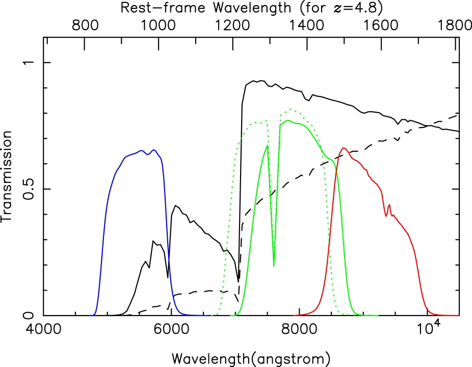
Figure 1: Effective transmissions (including quantum efficiency of the CCD and atmospheric absorption) for the three filters used in our observations (solid lines with blue ($V$), green ($I_{c}$) and red($z^{\prime}$)). The transmission of $i^{\prime}$ filter used in Ouchi et al. (2004a) is also shown as a dotted line. Model spectra of star-forming galaxies at $z=4.8$ are shown as black lines. The solid line represents the case without dust attenuation and the dashed line is for the case with $E(B-V)=0.4$. These SEDs are normalized at 10,000 Å. See text for details of the models. Upper-side ticks indicate rest-frame wavelengths for an object at $z=4.8$.

2.1 The Hubble Deep Field - North

We made deep imaging observations of the field that surrounds the HDF-N using the Suprime-Cam attached to the 8.2m Subaru Telescope in February 2001. The results presented in I03 are based on these data alone. For the new results we show in the present paper we also used the imaging data taken by the University of Hawaii (UH) group (Capak et al., 2004) using the same instrument and the same filters during February 28 – April 23, 2001. We retrieved these UH data from the SMOKA data archive (Baba et al., 2002).

Properties of these two sets of observations are different from each other in several aspects. First, the central field positions are $\sim$3′  apart, and in our observations the position angle was set to 10°(east of north), while in the observations by the UH group position angles were 0°or 180°. The position and the position angle in our observation were adjusted so that the HDF-N taken by the HST/WFPC2 was located at the centre of one of Suprime-Cam’s CCD chips. The dithering lengths are also different. In our observations dithering scales are only 10″–15″, which were chosen so that the area with deepest integration time became as large as possible. We could choose such small dither lengths because we concentrated on the detection of galaxies at $z\sim 5$, which should be apparently small ($\la 2\arcsec$). In the UH observations by Capak et al. (2004) the dither scales were around 1′and the effective exposure time within the observing field is fairly close to uniform. In this paper the area common to these two different sets of observations is used, since that area achieves the deep image depths in all of three observing bands ($V$, $I_{c}$ and $z^{\prime}$). In Table 1 we summarize observations for the HDF-N region.

2.2 J0053+1234

In order to increase the survey area and examine the effect of field-to-field variance, we carried out the imaging of another blank field. Specifically, we imaged the J0053+1234 region, which is one of the target fields of the Caltech Faint Galaxy Redshift Survey (Cohen et al. 1999a; Cohen et al. 1999b). Using extensive Keck spectroscopy, these authors identified 163 galaxies in the redshift range $0.173<z<1.44$ within an $2\arcmin\times 7.\arcmin 3$ field. Steidel et al. (1999, 2003) also selected this region as one of the target fields of their searches for LBGs at $z\sim 3$ and 4, and they identified 19 galaxies with spectroscopic redshifts at $3<z<5$.

Our imaging observations of this field using Subaru / Suprime-Cam have been executed during the summer seasons from 2002 to 2004. The central coordinate of the pointing is 00^h53^m23.0^s, +12°33′56″(J2000.0). In Table 2 we summarize information of our observations and final limiting magnitudes in $V$, $I_{c}$ and $z^{\prime}$. Although the point spread function of the final images are smaller than that in our images of the HDF-N region, the total limiting magnitudes achieved for this field are 0.3 – 0.5 mag shallower than those for the HDF-N region since the effective net exposure times are shorter due to the poor weather conditions we experienced. Nevertheless, these data more than double the total survey area and so are very valuable for populating the relatively rare, bright part of the sample and for examining field-to-field variations.

3 Data Reduction and Selection of LBG Candidates

3.1 Image Processing

The basic image processing was done using nekosoft — the software developed for the data reduction of mosaiced CCD cameras (Yagi et al., 2002) — as well as with IRAF. Bias was subtracted using overscan regions. Next, flat-field frames were generated by combining median-normalized object frames after masking objects. Then, after division by the flat-field frame and cosmic-ray removal (using CRUTIL in IRAF), a distortion correction was made for every frame with correction factors which were determined for each CCD position.

Image mosaicing in each band was made by identifying 40–180 stars common in object frames. The correction for differences in sensitivity and fluctuations of point source flux was also made based on these star data. In the HDF-N region, the data taken by us have small dither scales and so we could not adopt a mosaicing procedure usually executed in nekosoft, which determines relative positions of frames by common stars in different CCD chips. Thus, we first derived relative positions of frames taken by the UH group and generated a mosaiced image using the UH data alone. We then calculated the positions of the frames taken by us relative to that mosaiced image. The final mosaiced image was then made using both the UH and our data. Among the 10 CCD chips of the Suprime-Cam, one chip was not working during part of the observations of the HDF-N region. We also excluded data of another CCD chip in our data because there is not enough overlapping area between the positions of this chip and the UH data to allow us to determine reliable relative positions. In the J0053+1234 region data from all CCD chips were used. The effective survey areas (after masking bright objects) are 508.5 arcmin² (the HDF-N region) and 781.4 arcmin² (the J0053+1234 region). The FWHM values of point sources in the mosaiced images are about 1.1″for the HDF-N region and 0.9″for the J0053+1234 region (Tables 1 and 2).

3.2 Astrometry

The conversions from pixel coordinates in mosaiced CCD images to equatorial coordinates were made using the USNO-B1 catalog (Monet et al., 2003). In total 1,000 to 1,300 stars in the catalog were identified in the mosaiced image in each band, and polynomial coefficients up to third order were calculated. Internal position errors in coordinate conversions are less than 0.2″rms all over the images. Because these accuracies are almost identical to that of the USNO-B1 catalog itself, we expect that positional uncertainty due to the errors in the corrections for optical image distortions and those in the mosaicing process to be smaller than 0.2″.

3.3 Photometric Catalog

The determination of photometric zero points for the HDF-N region is described in I03 . Briefly, we determined photometric zero points based on imaging data of Landolt (1992) standard stars for $V$ and $I_{c}$ bands, while for $z^{\prime}$-band the zero point was determined through the distribution of $I_{c}-z^{\prime}$ colours of field stars and galaxies exposed on our images. Systematic errors in the determination of zero points are estimated to be 0.02, 0.08 and 0.1 mag for $V$, $I_{c}$ and $z^{\prime}$-bands, respectively. The photometric zero points of the final mosaiced images were determined by comparison with the images used in I03 . For the J0053+1234 region, the same procedure was followed for the $V$ and $I_{c}$ bands, while for $z^{\prime}$-band images of spectrophotometric standard stars taken during the same observing nights were used. Systematic errors are estimated to be 0.04 mag for $V$-band and 0.03 mag for $I_{c}$ and $z^{\prime}$-bands. Corrections for Galactic extinction were made based on the dust map by Schlegel et al. (1998). The amount of reddening for the HDF-N region is assumed to be $E(B-V)=0.012$, and for the J0053+1234 region it is $E(B-V)=0.066$.

Object detection and photometry were made by using SExtractor (Bertin and Arnouts, 1996) ver. 2.3 in single-image mode. A Gaussian filter with FWHM=3 pixels was used, and at least 4 contiguous pixels with counts higher than 1.3 $\sigma$ above background counts were required to be detected as an object. The cross-identifications of objects in our three bands were made in equatorial coordinates. Objects were included in the object catalog only when they were within the area with sufficient image depth, determined by checking the exposure maps which take account of the number of exposures and variations in sensitivity between individual CCD chips. This procedure guarantees that the image quality is fairly close to uniform and that the variance of photometric errors does not affect the uniformity of the galaxy sample. For $V$-band dropout LBGs we require objects to be detected both in $I_{c}$ and $z^{\prime}$-bands. We used MAG_AUTO as a total magnitude in all bands, and derived $V-I_{c}$ and $I_{c}-z^{\prime}$ colours using 1.6″diameter aperture magnitudes. Since object centroids are determined separately in each band, there is a possibility that the positions of apertures in different bands have offsets (e.g., star-forming regions are prominent in $I_{c}$-band and their distribution is irregular). We feel that such problems are rare, since FWHM sizes of LBG candidates are mostly smaller than the aperture size used to derive colours (1.6″). We also find through visual inspection that morphologies of $V$-dropout objects in $I_{c}$-band and in $z^{\prime}$-band are similar in most cases. The photometric catalogs of both fields were constructed based on the $z^{\prime}$-band. For objects undetected by SExtractor in the $V$-band, $V$-band aperture photometry was made at the objects’ positions in the $z^{\prime}$-band. In these cases, if the flux density within 1.6″diameter exceeded the 3-$\sigma$ sky fluctuation then the measured aperture magnitude was used to calculate $V-I_{c}$ colour. Otherwise the 3-$\sigma$ upper limit was adopted.

3.4 Selection of LBG Candidates

The colour criteria we adopted to select LBG candidates at $z\sim 5$ are the same as those used in I03 . They were defined to efficiently select star-forming galaxies at $z\sim 5$ without heavy contamination by objects from lower redshifts, and were chosen by considering the colours of both model galaxies and real galaxies within our images which have spectroscopic redshifts identified by previous surveys available at that time (see below for the cross-identifications of galaxies with spectroscopic redshifts with our object catalogues). Our colour criteria are expressed by the following equations in the AB magnitude system:

$$V-I_{c}>1.55$$

and

$$V-I_{c}>7.0(I_{c}-z^{\prime})+0.15.$$

In Fig. 2 we show our $z\sim 5$ colour selection criteria along with redshift colour tracks of several types of galaxies. The colour tracks of model star-forming galaxies are calculated based on the same SEDs as used in Fig. 1 (see section 2). Colour tracks for spiral (Sbc and Scd) and elliptical galaxies are calculated using template SEDs of local galaxies by Coleman et al. (1980).

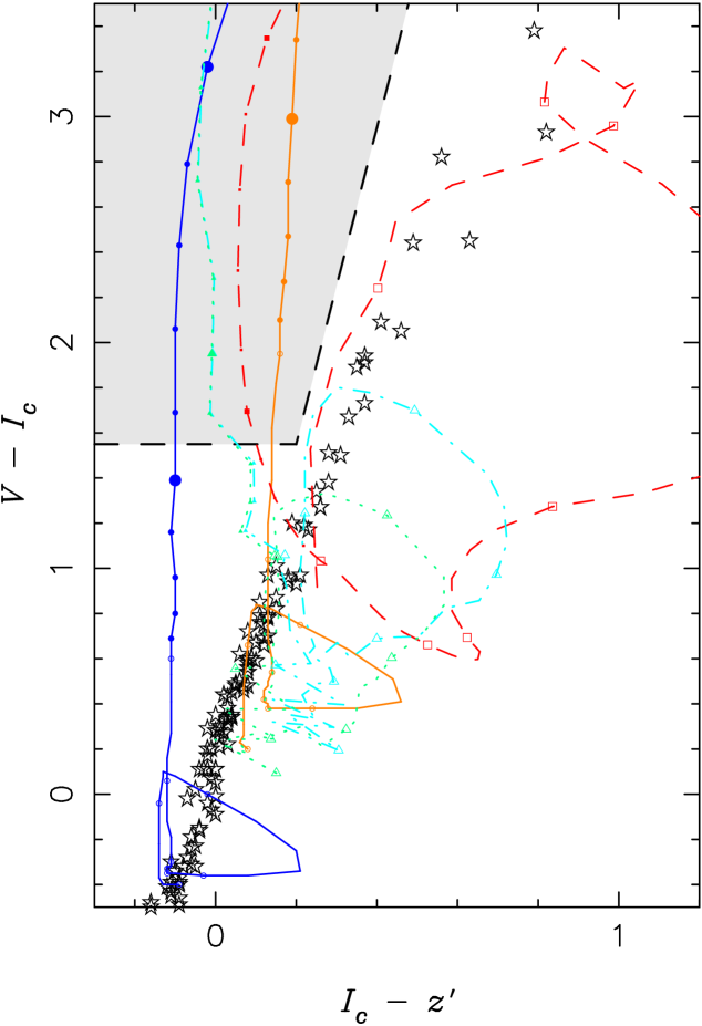
Figure 2: A $V-I_{c}$ and $I_{c}-z^{\prime}$ two colour diagram. The shaded area stands for the colour selection criteria adopted for the selection of Lyman break galaxies at $z\sim 5$. Lines are loci of colour changes for model galaxies along redshift. Solid blue: a star-forming galaxy without dust attenuation. Solid orange: a star-forming galaxy with dust attenuation of $E(B-V)=0.4$. Solid circles are plotted for $z\geq 4.1$ with an interval of 0.1. Symbols at $z=4.5$ and $z=5.0$ are enlarged. Colour tracks calculated using template SEDs by Coleman et al. (1980) are also shown. Cyan (dot-dashed): Sbc, light blue (dotted): Scd, red (dashed): elliptical. Symbols are plotted with a redshift interval of 0.5. Star symbols indicate the colours of A0–M9 stars calculated based on the library by Pickles (1998).

In Fig. 3 we show colours of detected objects within a magnitude range $23.0<z^{\prime}<24.5$. The numbers of objects which satisfy the colour criteria are 617 and 236 for the HDF-N region ($z^{\prime}<26.5$ mag) and the J0053+1234 region ($z^{\prime}<25.5$ mag), respectively.

Among the HDF-N field LBG candidates in I03 that are within the region common to the new, deeper and narrower imaging data, all of the objects with $I_{c}\leq 24.5$ mag and 82% of objects with $I_{c}\leq 26.0$ mag are included in our updated source catalog. The number of objects that were listed as LBG candidates in I03 but are outside the colour criteria in the new catalog is 20–30% larger than the estimated number of low-redshift contaminants (see section 4.1 and Table 5). This fact is not surprising, because the signal-to-noise ratios of our previous data are worse than the HDF-N region data presented in this paper.

Both of our target fields have been observed with other intensive spectroscopic surveys. We identified objects with spectroscopic redshifts in our images and plotted their colours in Fig. 3. For the HDF-N region we used the results of two surveys (Cohen et al. 2000 and Wirth et al. 2004). The numbers of objects identified are 644 for Cohen et al. (2000) and 1,803 for Wirth et al. (2004) (most of the objects in Cohen et al. 2000 are included in Wirth et al. 2004). In Fig. 3(a) we only show objects with $I_{c}>22.0$ mag and $V>22.0$ mag, because photometry of objects brighter than these limits would be unreliable due to saturation or detector non-linearity. Out of 1237 objects with spectroscopic redshifts smaller than 4.5, only two fall within our $z\sim 5$ colour selection criteria. Both of them have $z^{\prime}$-band magnitude $\approx 22$ and their redshifts are 0.32 (ID=7066 by Wirth et al. 2004) and 0.64 (ID=3249). For the J0053+1234 region, we show objects with published spectroscopic redshift smaller than 4.5 with magenta squares in Fig. 3(b). One sensible exception to this is CDFb-G5 at $z=4.486$, which satisfies our colour selection criteria ($V-I_{c}=2.70$, $I_{c}-z^{\prime}=0.29$) and is shown with a filled green circle as one of the spectroscopically confirmed LBGs at $z\sim 5$ (see section 3.5). In addition to this object, two objects at $z<4.5$ are within the colour selection criteria for $z\sim 5$ LBGs. One of them is object id D0K 163 in Cohen et al. (1999a). The redshift provided in Cohen et al. (1999a) is $z=0.580$ and is tagged with ’absorption only; faint; id uncertain’. It has a blue colour in $I_{c}-z^{\prime}$ (0.07) in our photometry. Another object is CDFa-GD12 in Steidel et al. (1999). The object is selected with their $z\sim 4$ LBG criteria (using $G$, $\cal R$, $I$ filters) and the spectroscopic redshift is $z=3.469$. Although the $I$-band magnitude listed in Steidel et al. (1999) is similar to our $z^{\prime}$-band magnitude ($z^{\prime}=24.76$ mag), the distance between the coordinate listed in Steidel et al. (1999) and ours are fairly large (1.74″), unlike other objects (mostly $<1\arcsec$).

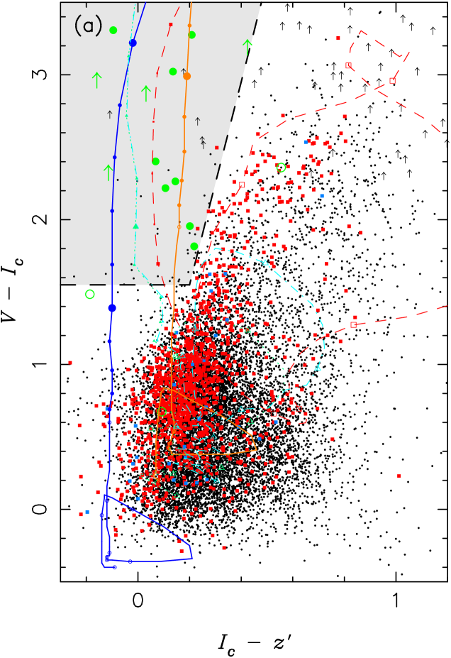
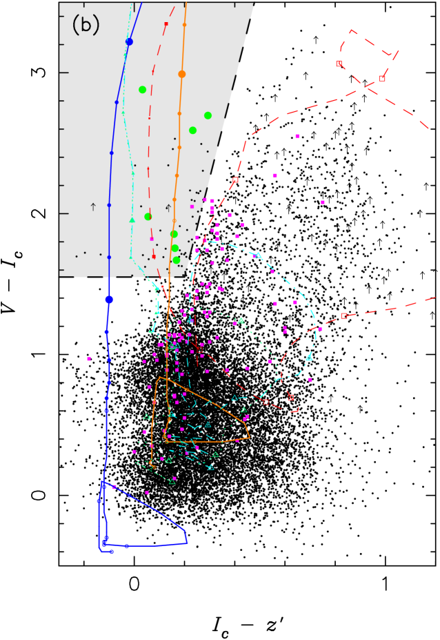
Figure 3: $V-I_{c}$ and $I_{c}-z^{\prime}$ two colour diagrams. (a): data points are for objects in the HDF-N region. Black circles indicate colours of objects with $23.0<z^{\prime}\leq 24.5$. For objects not detected in $V$-band, arrows are used to show the 3-$\sigma$ lower limits of $V-I_{c}$ colours. Red and blue squares represent galaxies with spectroscopic redshifts ($z<4.0$) published in Wirth et al. (2004) and Cohen et al. (2000) respectively. Objects in Cohen et al. (2000) which are listed in the catalog by Wirth et al. (2004) are omitted. Colour track lines and star symbols are the same as in Fig. 2. Filled green circles indicate colours of galaxies at $z>4.5$ confirmed by spectroscopy. Three open green circles show colours of objects which are not included in our LBG candidates catalog but are reported to be at $z>4.5$ in previous spectroscopic observations (see table 3). (b): same as (a) but for the J0053+1234 region. Squares in magenta are objects with spectroscopic redshifts smaller than 4.0 in the region, mostly taken from Cohen et al. (1999a), and green circles are galaxies at $z>4.2$ identified by spectroscopy by us and Steidel et al. (1999) (see table 4). See text for more details of these figures.

In I03 we defined the colour criteria for selection of $z\sim 5$ LBGs using the colours of galaxies with spectroscopic and photometric redshifts in the HDF-N region, as well as model colour tracks. Since the publication of I03 the number of low-redshift galaxies with spectroscopic identifications in the HDF-N region has greatly increased, but, as described above, the cross-identification of these spectroscopic samples with our LBG catalog shows that the number of low-redshift galaxies that contaminate our colour selection criteria is very small.

Since the magnitude range of our LBG candidates is fainter than most of these spectroscopically identified low-redshift objects, the objects identified as contaminants cannot be used to estimate the fraction of contaminants in our sample. Consequently, we need resampling tests to estimate the contamination fraction as a function of magnitude, as described in section 4.1.

Our HDF-N region contains the GOODS-N area, where deep HST/ACS and Spitzer/IRAC and MIPS imaging have been made (Giavalisco et al. 2004a). The ACS images are in the $B_{\mathrm{435}}$, $V_{\mathrm{606}}$, $I_{\mathrm{775}}$ and $z_{\mathrm{850}}$ filters and using $V_{\mathrm{606}}$, $I_{\mathrm{775}}$ and $z_{\mathrm{850}}$, a $V$-dropout LBG sample has been constructed (Ravindranath et al., 2006). However, it is not straightforward to compare our sample with those based on the ACS images. Since the filters used are different, especially $V_{\mathrm{606}}$ which has a very broad bandpass (width is $\simeq 1500\mathrm{\AA}$), the colour tracks of the same galaxy SEDs with GOODS/ACS filters in the two-colour diagram are quite different from ours.

In Fig. 4 the sky distributions of LBG candidates in our two fields are shown. There is a clear fluctuation in surface density of LBG candidates; some areas have many LBGs while others don’t, and these irregularity in the surface density is not caused by the masks used to avoid effect of foreground bright objects such as galactic stars and nearby galaxies. Fairly strong clustering signals have been found with past wide-field LBG searches (e.g., Giavalisco et al. 1998; Adelberger et al. 1998; Foucaud et al. 2003; Ouchi et al. 2004b; Hamana et al. 2006). These figures also tell us that in small-area surveys such as the HDF-N, the Hubble Ultra Deep Field and even GOODS, the effect of field-to-field variance would be much more serious than for our data. Detailed analyses of clustering properties of our LBG samples will be presented in a forthcoming paper.

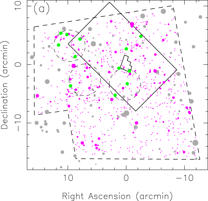
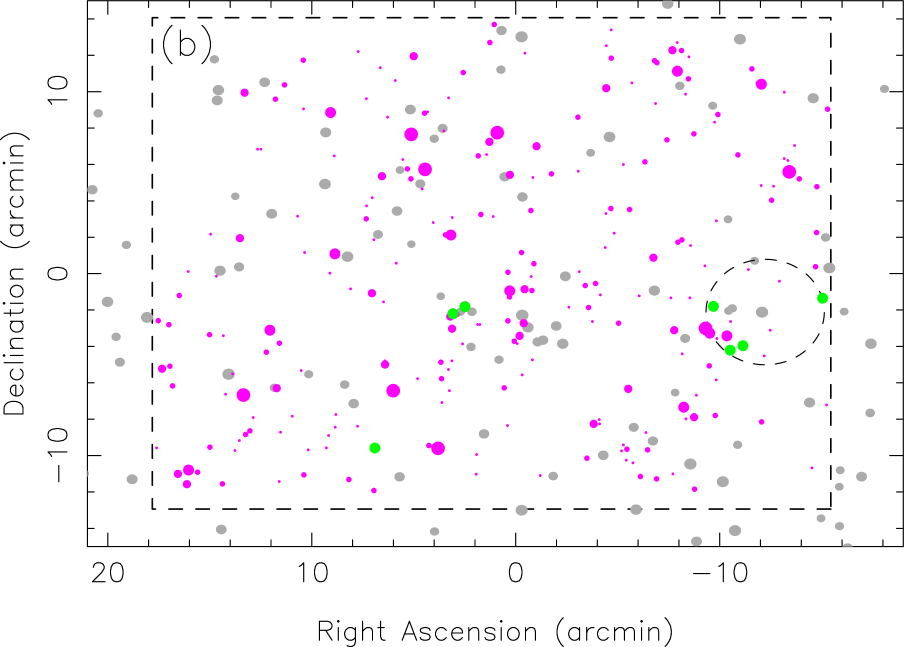
Figure 4: Sky distribution of LBG candidates in the HDF-N region (a) and in the J0053+1234 region (b). Filled magenta circles show the positions of LBG candidates. Symbol size indicates objects’ brightness in a 0.5 mag step. Filled green circles are for objects which have been confirmed to be at $z\ga 4.5$ with optical spectroscopy. Large circles with dashed lines indicate the positions and areas of optical spectroscopy by us. Gray circles indicate the position of masks used to avoid the effects of bright stars. Rough boundaries of image areas used for selection of LBG candidates are shown with dashed lines. Note that not all of the area within these lines is used: due to the gaps between CCD chips, different position angles and dither scale lengths, some positions near boundaries have smaller effective exposure time, and such areas were not used for candidate selection. Large and small areas drawn with solid lines in Fig. 4(a) are the HST survey areas of the GOODS-N and the HDF-N, respectively.

3.5 Spectroscopic Identifications of Galaxies at $z\sim 5$

We carried out optical spectroscopic observations using a multi-object spectroscopy mode of the FOCAS (Kashikawa et al., 2002) attached to the Subaru telescope. Until now, 8 objects in the HDF-N region and 4 objects in the J0053+1234 region have been identified to be in the redshift range between $z=4.2$ and 5.2 (Ando et al. 2004; Ando et al. 2007; including one AGN GOODS J123647.96+620941.7). No object with smaller redshift has been found in our observations so far, although more than half of the observed spectra have too low a signal-to-noise ratio to determine their redshifts. Four objects which have slightly redder $I_{c}-z^{\prime}$ colours than the colour selection criteria have been identified as Galactic M-type stars (Ando et al., 2004).

In addition, there are 8 objects in the HDF-N region and 2 objects in J0053+1234 which have been spectroscopically identified to be at $4.5<z<5.5$ by other researchers. Among them, 6 objects are selected as $V$-dropout candidates in our images. Tables 3 and 4 provide summaries of the cross-identifications of these objects with previously published spectroscopic redshifts. In Fig. 3, the objects that have been selected as $V$-dropout candidates in our images and that have spectroscopic confirmations are shown with filled green circles (or upper arrows for objects not detected in $V$-band). There are four objects in the HDF-N region which have been previously reported to have spectroscopic redshifts larger than 4.5 and are detected in our images but do not satisfy our colour selection criteria (see table 3). Their positions in the $V-I_{c}$ and $I_{c}-z^{\prime}$ diagram are shown as open circles in Fig. 3. The first of these, HDF-N 4-439.0 at $z=4.54$, has $V-I_{c}=1.48$ and is slightly off from our colour selection window. Another object, F36219$-$1516, which has been reported to be at $z=4.89$ by Dawson et al. (2001), has a very blue $V-I_{c}$ colour in our image ($V-I_{c}=0.67$). Since the redshift determination was made with solely a single emission line (identified as Ly$\alpha$), we suggest that this may be a misidentification of a lower redshift object. F36376$-$1453 is another object with a single emission line in the spectrum which was identified as Ly$\alpha$ at $z=4.886$ by Dawson et al. (2001). This object is very bright ($z^{\prime}=21.97$) and its colours in both $V-I_{c}$ and $I_{c}-z^{\prime}$ are red ($V-I_{c}=3.25$, $I_{c}-z^{\prime}=0.78$ and this object is outside of plotted area of Fig. 3). It has a round shape in our images in $I_{c}$ and $z^{\prime}$-bands (FWHM$\sim 1.0^{\prime\prime}$). The fourth object, GOODS J123721.03+621502.1, was identified as an object at $z=4.76$ by Cowie et al. (2004) (no. 1173 in their table 1). This object also has red colours in $V-I_{c}$ and $I_{c}-z^{\prime}$. No information about the quality of the spectrum is provided in Cowie et al. (2004). On the other hand, one object in the J0053+1234 region which is at $z=4.486$ (CDFb-G5 in Steidel et al. 1999) and is within our selection window ($V-I_{c}=2.70$, $I_{c}-z^{\prime}=0.29$; see table 4), and it is shown as an filled green circle in Fig. 3(b). In summary, spectroscopic observations for our LBG candidates still cover only a small fraction of the sample, but the results obtained so far are encouraging. Both the existence of objects at $z\sim 5$ within the selection window and the small number of contaminants described in section 3.4 strongly support the validity of our selection criteria.

Capak et al. (2004) analysed multicolour data including some of the same Suprime-Cam data that we now re-processed and included in the present work to construct our multi-band object catalog in the HDF-N region. They also made a selection of $V$-dropout galaxies, derived their number counts, and compared them with those in I03 . The number counts in Capak et al. (2004) are just 13–21% of those in this paper. They claimed that our sample may be contaminated by $z\simeq 1$ galaxies since our selection criteria are redder than theirs in $I_{c}-z^{\prime}$ colour. However, their arguments are incorrect. The colour criteria used in Capak et al. (2004) are $V-I_{c}\geq 2.4$ and $V-I_{c}\geq 7(I_{c}-z^{\prime})-0.2$ and the latter criterion is slightly redder than ours (in both I03 and the present paper we use $V-I_{c}>7.0(I_{c}-z^{\prime})+0.15$ when on the AB normalization), contrary to their argument. Instead, the main cause of the small number counts with their selection is that their first criterion sets too strong a lower limit in $V-I_{c}$ colour and thus misses many $z\simeq 4.5$ galaxies. As is shown in Fig. 3, their criterion, $V-I_{c}\geq 2.4$, misses many LBGs with high-$z$ spectroscopic identifications.

3.6 UV colour distribution

If our LBG candidates are real objects at $z\sim 5$ then their $I_{c}-z^{\prime}$ colours represent rest-frame UV colours. In Fig. 5 we show the distribution of $I_{c}-z^{\prime}$ colours along apparent $z^{\prime}$-band magnitude. In this figure we also show the distribution of $I_{c}-z^{\prime}$ colours for objects with $23.0<z^{\prime}<26.0$ as filled circles and the median colour values in different $z^{\prime}$-band magnitudes (in a 0.5 mag step) as squares. Typical photometric errors in $I_{c}-z^{\prime}$ colours are calculated from the simulations using artificial objects (described in section 4.1), assuming $I_{c}-z^{\prime}=0.07$ mag (from a model SED at $z=4.8$, $E(B-V)=0.2$). Because upper limits on $I_{c}-z^{\prime}$ colour values are imposed during the selection of LBGs, there are few objects with $I_{c}-z^{\prime}>0.4$. This does not mean that all star-forming galaxies at $z\sim 5$ have such blue UV colours. We do not know what fraction of star-forming galaxies with red UV colours (probably due to heavy attenuation by dust) at the target redshift are missed in our search; at least in the redshift range $z=2$–3 significant populations of star-forming galaxies with redder rest-frame UV colour have been detected (e.g, Förster Schreiber et al. 2004; Daddi et al. 2004). Application of similar methods at higher redshifts will be an important subject of future space-based infrared missions, but for now we must press on with UV-selected samples.

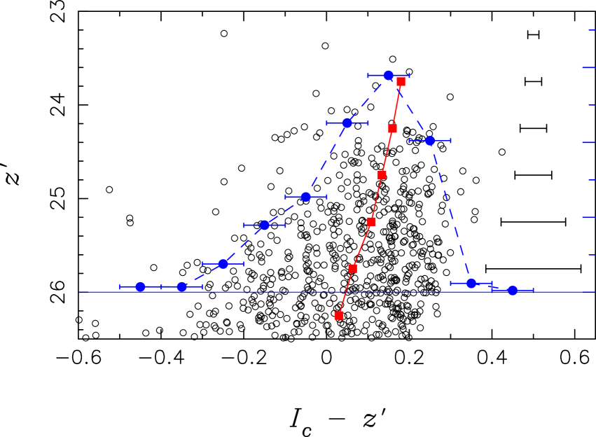
Figure 5: $z^{\prime}$-band magnitude against $I_{c}-z^{\prime}$ colour for LBG candidates at $z\sim 5$ in the HDF-N region. Open circles show magnitudes and colours of individual galaxies. Typical errors in $I_{c}-z^{\prime}$ colours are displayed in the right side of the panel. Solid squares show the median of $I_{c}-z^{\prime}$ colours in a 0.5 mag step in $z^{\prime}$-band magnitude. Filled circles indicate the distribution of fraction of $I_{c}-z^{\prime}$ colours in an 0.1 dex step for objects with $23.0<z^{\prime}<26.0$, and its scale is shown in the right side vertical axis.

In the median values of $I_{c}-z^{\prime}$ colours there is a weak trend in that objects bright in $z^{\prime}$-band have redder $I_{c}-z^{\prime}$ colours. In other words, the ratio of the number of blue (e.g., $I_{c}-z^{\prime}<0$) objects to the number of red objects is smaller for bright objects than for fainter ones. Since the upper limit on $I_{c}-z^{\prime}$ colour in our selection criteria depends on $V-I_{c}$ colour, the selection effect is not straightforward in this figure. However, since there is no restriction for the selection of objects with blue $I_{c}-z^{\prime}$ colours, the absence of bright objects with blue rest-frame UV colour must be real. There is no selection bias due to the limiting magnitude in $I_{c}$-band, since this is $I_{c}=26.86$ mag in the HDF-N region. The red colour of UV continua can be attributed to various origins, including heavier dust attenuation, older stellar populations, and weaker Lyman $\alpha$ emission (for objects at $z>4.8$ the $I_{c}$ filter covers the rest-frame Lyman $\alpha$ wavelength). We will briefly discuss this dependence of the UV colour distribution on UV luminosity in section 5.2.2.

4 UV Luminosity Function at $z\sim 5$

4.1 Correction for Incompleteness and Contamination

The procedure that we use to derive the UV luminosity function follows that described in our previous paper (I03, ) which was based on shallower data for the HDF-N region only. To estimate the volumes sampled with our adopted colour criteria, we execute a large set of tests in which we use artificial galaxies which mimic the size distribution of real galaxies in our sample. We are able to derive the completeness of our survey for objects with specific magnitudes and colours by counting the number of artificial objects which have been recovered by the object detection and colour selection procedures. In a single test run we generate 25,000 artificial objects for each bin of 0.5 in magnitude, 0.1 in redshift, and reddening by dust (five different degree of reddening from $E(B-V)=0.0$ to 0.4 with steps of 0.1). Colours are assigned based on the model spectra of star-forming galaxies generated with PEGASE.2 (see Fig. 2), Calzetti et al. (2000) extinction law, and a prescription for IGM attenuation by Inoue et al. (2005). These objects are then put into random positions in the $V$, $I_{c}$ and $z^{\prime}$ images. The methods of object detection and sample selection according to the colour criteria are the same as those for real objects, described in sections 3.3 and 3.4.

In Fig. 6 we show the completeness of our survey as a function of redshift and $z^{\prime}$-band magnitude. Results for five different amounts of reddening were averaged with weights estimated from the UV colour distribution of real galaxies (section 3.6). The maximum completeness is achieved for brightest (23.0–23.5 mag) objects at redshift 4.5–5.0 in the HDF-N region. We note that there is a significant ($\ga 10$%) detection rate for objects at $z\sim 4$. It suggests that in our sample of $z\sim 5$ LBG candidates there should be a small number of objects at such lower redshift ranges. So far we have detected one object at $z=4.26$ in the optical spectroscopy of the J0053+1234 region (table 4; Ando et al. 2007). The existence of such relatively low redshift objects does not have a serious effect in deriving the UVLF at $z\sim 5$, since we properly treat them by calculating the survey volume using these selection functions. The detection rates in the J0053+1234 region are lower than those in the HDF-N region at the same magnitude ranges, and they are similar to those for the data used in I03 , which were $\sim 0.8$ mag shallower in $z^{\prime}$-band than the present HDF-N data.

Figure 6: Detection rates of the galaxies for the HDF-N region (solid lines) and the J0053+1234 region (dashed lines), as a function of $z^{\prime}$-band magnitude and redshift. The lines represent $z^{\prime}$-band magnitude of 23.0–23.5, 24.0–24.5, 25.0–25.5 and 26.0–26.5 (the last bin for the HDF-N region only).

A weighted average value of redshift derived from this completeness distribution is 4.8 for both the HDF-N and the J0053+1234 regions. Hereafter we use this value as a typical redshift in the presentation of the UV luminosity function. From these completeness estimates for different magnitudes, redshifts and amount of dust reddening, we calculated the effective volumes (Steidel et al., 1999) of our surveys, which are listed in Tables 5 and 6.

As we did in I03 , we use a resampling method to estimate the rate of contamination by galactic stars and galaxies at intermediate redshifts. We perturbed the colours of detected objects which lie outside of the colour selection criteria by adding random errors based on the error measurements in photometry. Then we counted the number of objects which fell into the colour selection criteria after the addition of these random errors. For each bin of 0.5 magnitude these resampling tests were executed 1,000 times, and average numbers of interlopers were derived. These numbers are listed in Table 5 and 6 as $N_{\mathrm{int}}$.

We compute the UVLF as

$$\Phi(m)=2\times(N(m)-N_{\mathrm{int}}(m))/V_{\mathrm{eff}}(m),$$

where $N(m)$ represents the number of LBG candidates detected within the magnitude bin of $m\pm 0.25$ mag, and $V_{\mathrm{eff}}(m)$ is the effective volume. The multiplication by 2 is required to obtain number densities per magnitude, since we take 0.5 mag bins in our sample. The UVLFs derived for the HDF-N region and the J0053+1234 region are listed in Tables 5 and 6, respectively, and they are shown in Fig. 7 with open circles (HDF-N) and open triangles (J0053+1234). The error bars indicate 1$\sigma$ error estimates including statistical (Poisson) noise, photometric errors and uncertainties in contaminations and completeness. In converting from apparent $z^{\prime}$-band magnitude to absolute magnitude we assume a luminosity distance of an object at $z=4.8$ under the adopted cosmology ($M_{\mathrm{U}V}=m_{z^{\prime}}-46.33$, $\Omega_{M}=0.3$, $\Omega_{\Lambda}=0.7$, $H_{0}=70$ km/s/Mpc). In I03 we made a correction for luminosity in the conversion from $I_{c}$-band apparent magnitude to rest-frame luminosity at 1700$\mathrm{\AA}$, assuming the SED of a model star-forming galaxy. In the present analysis we do not make such a correction in the conversion from magnitudes in $z^{\prime}$-band (the effective wavelength is $9086\mathrm{\AA}$), and thus the LFs we present are at $\approx 1570\mathrm{\AA}$.

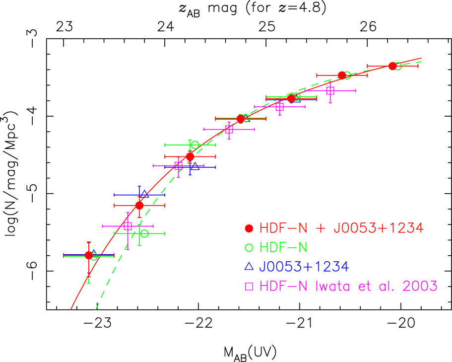
Figure 7: UV luminosity functions (UVLFs) at $z\sim 5$. Open circles and open triangles represent UVLFs of LBGs at $z\sim 5$ in the HDF-N region and the J0053+1234 region, respectively. Filled circles show the UVLF derived by combining results of the two fields. The data points of UVLFs based on single fields are shifted +0.05 mag for clarity. The solid line represents the Schechter function fitted to the combined UVLF, and the dashed line is a fitting for the UVLF in the HDF-N. Open squares are the UVLF in the HDF-N region determined with previous shallower data (I03).

In the calculation of selection functions and effective volumes we assume a dust attenuation distribution from $E(B-V)=0.0$ to 0.4 based on the $I_{c}-z^{\prime}$ colour distribution. In order to examine the robustness of the LF against this assumption about dust attenuation, we also calculated effective volumes with two extreme cases in dust attenuation: one case is that using just a model without dust attenuation ($E(B-V)=0.0$) and the other is only using a model with relatively large dust attenuation ($E(B-V)=0.4$). In these extreme cases the shape of selection function along redshift changes from that shown in Fig. 6, because the redshift range covered with our selection criteria changes when the assumed model is different. However, we find that the differences in the resulting LF — even with these extreme cases — are small, as shown in Fig. 8. In this figure the UVLFs in the HDF-N region using effective volumes calculated based on these extreme assumptions are compared with the UVLF computed using the fiducial dust attenuation distribution. Since the extreme assumptions in these tests (all objects are free from dust or all objects have fairly large dust attenuation of $E(B-V)=0.4$) are unlikely, we can say that our UVLF is robust against the assumption of model colours and distribution of amount of dust attenuation.

The modification of the selection criteria should also alter the effective volume. We examined the change of effective volumes and luminosity function by means of a test in which the colour selection criteria were shifted in both $V-I_{c}$ and $I_{c}-z^{\prime}$ with 0.05–0.15 magnitude, and derived luminosity functions in the same way as we did for the original selection criteria. The UVLFs obtained by these tests show differences smaller than the error bars of our LF shown in Fig. 7. With these tests we verified that our UVLF results are robust against slight changes to the colour selection criteria.

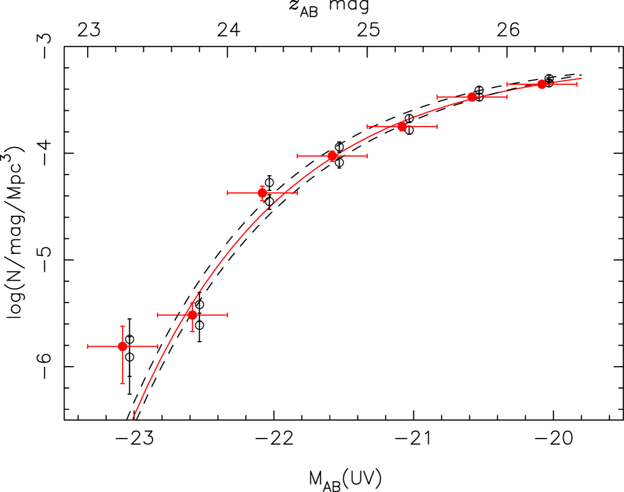
Figure 8: The UVLF at $z\sim 5$ for the HDF-N region (same as the UVLF with open circles in Fig. 7) calculated using the distribution of dust attenuation estimated from $I_{c}-z^{\prime}$ colours (Fig. 5) is compared with UVLFs derived based on two extreme assumptions about the dust attenuation of our sample LBGs (no attenuation and $E(B-V)=0.4$ for all objects), shown with open circles. LFs with open circles are shifted +0.05 mag for clarity. See section 4.1 for details.

4.2 Combination of the UVLFs in the two survey fields and Schechter function fitting

Since the J0053+1234 sample is shallower than the HDF-N sample, the UVLF of the J0053+1234 region is limited to $z^{\prime}<25.5$ mag. As shown in Fig. 7, the number densities of these two fields agree fairly well, although in two bright magnitude bins ($23.5<z^{\prime}<24.0$ and $24.0<z^{\prime}<24.5$) the discrepancy between results from the two fields is large enough that it exceeds the size of the 1-$\sigma$ error bars. This is probably due to the small number of objects (5–35) in these magnitude bins, and it might also indicate the existence of field-to-field variations, the effect of which is not included in the error estimates.

We averaged the number densities of the two fields by applying weights based on their survey areas (for magnitude range brighter than $z^{\prime}=25.5$), and derived the final UVLF with the present data set. This UVLF is listed in Table 7 and is shown as filled circles in Fig. 7. Hereafter we call this the final UVLF.

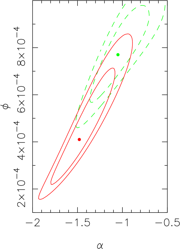
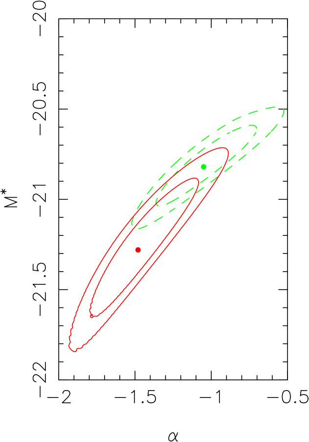
Figure 9: Confidence contours of Schechter function parameters. Solid lines show areas show the 68% (inner) and 95% (outer) confidence levels for the ’final’ UVLF which combines the results of the two fields. Dashed lines are the same as the solid lines, but for the (deeper) HDF-N data only. Small points show the values of the best-fitted parameters.

The results of fitting the UVLFs with the Schechter function (Schechter, 1976) are also shown in Fig. 7. The solid line is a function fitted to the final UVLF, and the dashed line is for the UVLF based solely on the deeper HDF-N region data. The best-fitted parameter values for the final UVLF and for the LF from the HDF-N region are summarized in Table 8. We note that the $z\sim 5$ Schechter parameter fit given in Sawicki and Thompson (2006b) is based on a (slightly earlier) version of the HDF-N region UVLF presented here. Fig. 9 also shows the 68% and 95% confidence level error contours calculated via Monte-Carlo resampling of the UVLFs. For each point of the observed UVLFs we add a random error according to its uncertainty (assuming Gaussian distribution), and execute the Schechter function fitting to this perturbed UVLF and obtain a $\chi^{2}$ value. We repeat this test 1,000 times and derive the region in parameter space that contains 68% or 95% of these resampling results.

Although the number densities in the combined data and those in the HDF-N region are fairly close in the fainter part of the LF ($24.0<z^{\prime}<25.5$), the best-fitted Schechter function parameters are significantly different. This difference is caused by relatively large difference in the number density in the bright $23.5<z^{\prime}<24.0$ magnitude range. Even the faint-end slope $\alpha$ is affected by the change in the LF’s bright part, due to changes in $\phi^{\ast}$ and $M^{\ast}$. The large field-to-field variation in the bright end of the UVLF between our two survey areas (both fields have areas larger than 500 arcmin²) clearly indicates the necessity of a large survey area and multiple survey fields. A study based on a single field observation may be affected by large-scale structure in the galaxy distribution. Moreover, if the survey area is small, it is very likely that the survey fails to detect bright and rare objects and so underestimates their number density. We also note that the Schechter function parameters are not a good way to represent the properties of observed LFs unless an observation reaches far deeper than $M^{\ast}$. A comparison of LFs at different epochs or in different environments should be cautious of uncertainties and degeneracy between parameters (as illustrated in Fig. 9). The direct comparison of number densities at in a fixed luminosity range is a better way to compare LFs.

4.3 Comparisons with UVLFs in previous studies of galaxies at $z\sim 5$

4.3.1 Comparison with the UVLF in Iwata et al. (2003)

The new UVLFs at $z\sim 5$ agree well with our previous result (I03, ) based on shallower data in the HDF-N region, which is indicated as open squares in Fig. 7. Note that because in I03 we used the Vega-based magnitude system and the fiducial redshift was $z=5.0$, the magnitude bins are slightly different from our present results.

4.3.2 Comparison with the UVLF of FORS Deep Field

In Fig. 10 we compare our UVLF with the one at 1500 Å which is based on the photometric redshift sample selected in $I$-band by Gabasch et al. (2004a). These authors used 150 galaxies in the FORS Deep Field (FDF) with $I$-band magnitudes brighter than 26.8 mag which have estimated redshifts between 4.01 and 5.01. While the depth of their sample is comparable to ours, the number of objects is small, mainly due to their small survey field area ($7^{\prime}\times 7^{\prime}$). The overall shape of the UVLF derived by Gabasch et al. (2004a) is similar to ours. The number density of faint galaxies in our UVLF at $z\sim 5$ is slightly smaller, as has been pointed out by Gabasch et al. (2004a) who used our previous UVLF for the comparison. Since the redshift range of galaxies in Gabasch et al. (2004a) is smaller than ours, this trend might indicate a real number density evolution of UV-selected star-forming galaxies (see section 5.1 for discussion of the differential UVLF evolution), although the difference in the methods of sample selection and possible field-to-field variation prevent us to make further discussions.

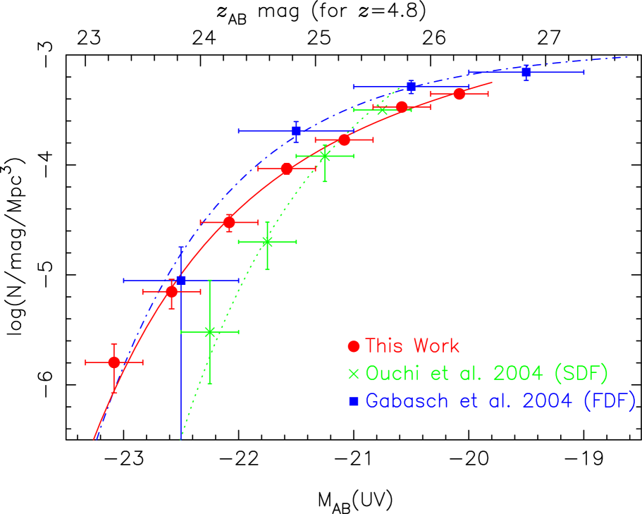
Figure 10: UV luminosity functions at $z\sim 5$. Filled circles show our UVLF derived by combining results of the two fields. This is the same UVLF as in Fig. 7. The solid line represents the Schechter function fitted to this combined UVLF. Solid squares represent the rest-frame 1500Å luminosity function derived by Gabasch et al. (2004a) from their $I$-band selected photometric redshift sample with estimated redshifts at $4.01<z<5.01$, and the dot-dashed line is a Schechter function fitted to it. The crosses are the UVLF for LBGs at $z\sim 5$ ($V$-band drop LBGs) by Ouchi et al. (2004a) and the dotted line represents the Schechter function fitted to their data with the faint-end slope fixed to $\alpha=-1.6$.

4.3.3 Comparison with the result of Subaru Deep Survey

In Fig. 10 we show with crosses the UVLF of LBGs at $z\sim 4.7$ derived by Ouchi et al. (2004a) in the Subaru Deep Field and show their fitted Schechter function using the dotted line. Note that their faint-end slope $\alpha$ was fixed to $-1.6$. As described in Ouchi et al. (2004a), there is a discrepancy in the bright part ($M_{\mathrm{UV}}<-21.5$ mag) between our previous UVLF (I03, ) and their result. The discrepancy still remains when our updated data is compared with the Ouchi et al. (2004a) UVLF, and this seems somewhat unnatural, since the field-to-field variance between our two survey fields (at $M_{\mathrm{UV}}<-22$) is more than three times smaller than the difference between our UVLFs and the one by Ouchi et al. (2004a). Recently, Yoshida et al. (2006) derived an updated UVLF of $z\sim 5$ LBGs in the same Subaru Deep Field using a deeper and $\approx$160 arcmin² wider image data set. Their filter set, procedures for reducing data, selecting LBG candidates, and calculating the UVLF are basically the same as those in Ouchi et al. (2004a). Consequently, their results agree with those by Ouchi et al. (2004a) and thus the number densities in their LF’s bright part remains significantly smaller than ours.

We further investigated the origin of the difference between our results and those by Ouchi et al. (2004a). One possible cause of this discrepancy is the difference in colour selection criteria. However, we must take care here because the filters used by us and those used by Ouchi et al. (2004a) are different: Ouchi et al. (2004a) used $i^{\prime}$ while we used $I_{c}$, and since the $i^{\prime}$-band filter has transmission that is shifted slightly to a shorter wavelength with respect to the $I_{c}$-band (see Fig. 1), the comparison of sample selection criteria is not straightforward. We illustrate this problem as follows. In Fig. 11 we use a dot-dashed line to show the $V-i^{\prime}$ and $i^{\prime}-z^{\prime}$ colour criteria used in Ouchi et al. (2004a). Fig. 11 also shows the redshift tracks of star-forming galaxies in the colour pair $V-I_{c}$ and $I_{c}-z^{\prime}$ (solid lines) and in the colour pair $V-i^{\prime}$ and $i^{\prime}-z^{\prime}$ (dashed lines). Since the effective wavelength of $i^{\prime}$-band is slightly shorter than that of $I_{c}$-band, the $i^{\prime}-z^{\prime}$ colour becomes red at relatively low redshift (at $z\sim 4.7$). If we were to apply the Ouchi et al. (2004a) criteria directly to our $V-I_{c}$ and $I_{c}-z^{\prime}$ colours, then the sample would be contaminated by many low-$z$ galaxies and galactic stars with $V-I_{c}\ga 2.4$ and $I_{c}-z^{\prime}\ga 0.4$, as shown with red squares and star symbols in Fig. 11(a). However, the selection criteria adopted by Ouchi et al. (2004a) avoid including these objects because the $i^{\prime}-z^{\prime}$ colours of these objects are $\sim 0.2$ mag redder than their $I_{c}-z^{\prime}$ colours. This illustrates the difficulty in making a direct comparison of the colour selection criteria of the two surveys.

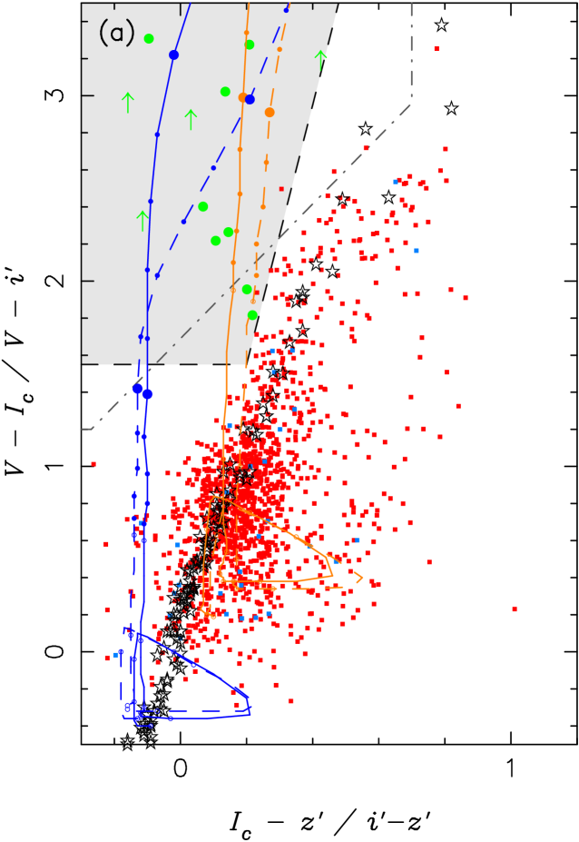
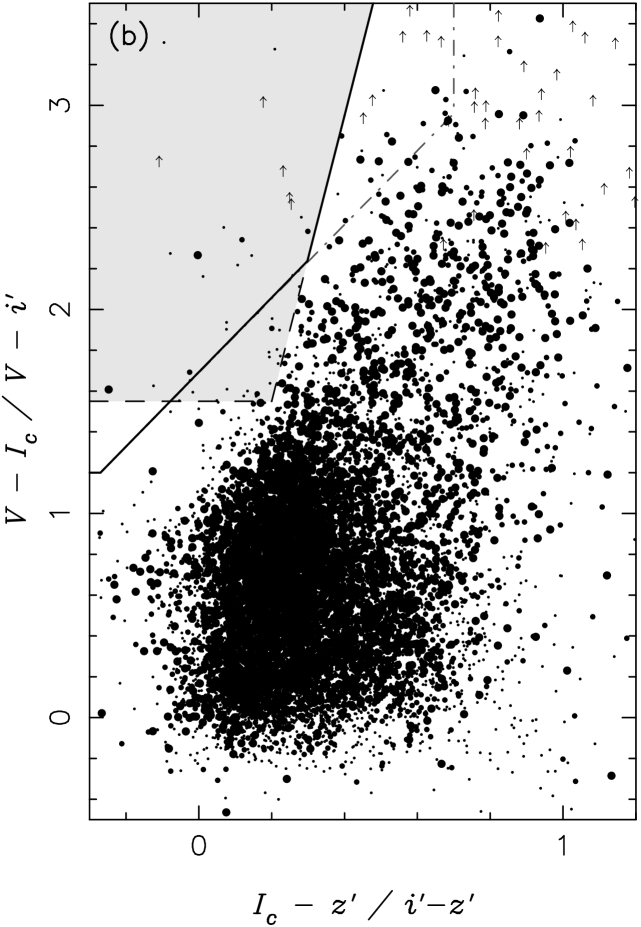
Figure 11: $V-I_{c}$ and $I_{c}-z^{\prime}$ two colour diagrams. (a): Red and blue squares are galaxies at $z<4.0$ in the HDF-N region, same as in Fig. 3a. Green circles are spectroscopically confirmed objects at $z>4.5$ in the HDF-N. For objects not detected in $V$-band, arrows are used to show the 3-$\sigma$ lower limits of $V-I_{c}$ colours. The dashed line and shaded area stands for colour selection criteria adopted in this study for the selection of Lyman break galaxies at $z\sim 5$. The colour selection criteria of Ouchi et al. (2004a) (used with $V-i^{\prime}$ and $i^{\prime}-z^{\prime}$ colours) are displayed with a dot-dashed line. Blue lines are colour tracks of a star-forming galaxy without dust attenuation, and lines in orange are for dust attenuation of $E(B-V)=0.4$. Solid lines show colours in $V-I_{c}$ and $I_{c}-z^{\prime}$, and dashed lines are in $V-i^{\prime}$ and $i^{\prime}-z^{\prime}$. Star symbols indicate the $V-I_{c}$ and $I_{c}-z^{\prime}$ colours of A0–M9 stars calculated based on the library by Pickles (1998). (b): same as (a), but shows objects with $23.0<z^{\prime}<24.5$ mag detected in our $V$, $I_{c}$ and $z^{\prime}$-band images for the HDF-N region. Sizes of symbols indicate object brightness in 0.5 mag bins, with the largest symbols representing objects with $23.0<z^{\prime}<23.5$ mag. The thick solid line represents the modified colour selection criteria used for the test described in section 4.3.3., which consist of the colour selection criteria of Ouchi et al. (2004a) for $i^{\prime}-z^{\prime}<0.3$, and for $i^{\prime}-z^{\prime}>0.3$ follows our colour selection criterion.

Thus, in order to roughly estimate the effect of the difference between colour selection criteria, we adopt modified criteria which consist of those used by Ouchi et al. (2004a) at $I_{c}-z^{\prime}<0.3$ and those used by us at $I_{c}-z^{\prime}\geq 0.3$. These modified criteria are shown with a thick solid line in Fig. 11(b); they approximately reproduce the Ouchi et al. (2004a) criteria as applied to our $V-I_{c}$, $I_{c}-z^{\prime}$ data. In Fig. 12 we show $z^{\prime}$-band number counts of LBGs in our survey fields, using both our criteria and the modified criteria of Ouchi et al. (2004a) and compare them with the number counts given by Ouchi et al. (2004a) and Yoshida et al. (2006). The change of colour selection criteria reduces the number of LBGs in the HDF-N region, but there remains a clear discrepancy between our number counts and those in the Subaru Deep Field (Ouchi et al. 2004a and Yoshida et al. 2006). In the 875 arcmin² of Yoshida et al. (2006) there is only one object with $z^{\prime}<24.05$ mag and only 12 objects with $z^{\prime}$-band magnitude between 24.05 and 24.55, while there are 7 objects with $z^{\prime}<24.0$ mag and 35 objects with $24.0<z^{\prime}<24.5$ mag in the HDF-N region when we use our own selection criteria. As shown in Fig. 11(b), when we adopt the modified colour criteria, six out of 7 LBG candidates with $23.0<z^{\prime}<24.0$ remain within the selection area. In $24.0<z^{\prime}<24.5$ the number of objects becomes 17, about half of our original sample, but this corresponds to $\approx 29$ for the survey area of Yoshida et al. (2006) and so represents a surface number density more than two times larger than theirs. Thus, the modification in the colour selection criteria is unable to explain the differences between the number densities in our final UVLF and those in the Subaru Deep Field, which are 2–5 times larger than the 1$\sigma$ errors estimated for our UVLF.

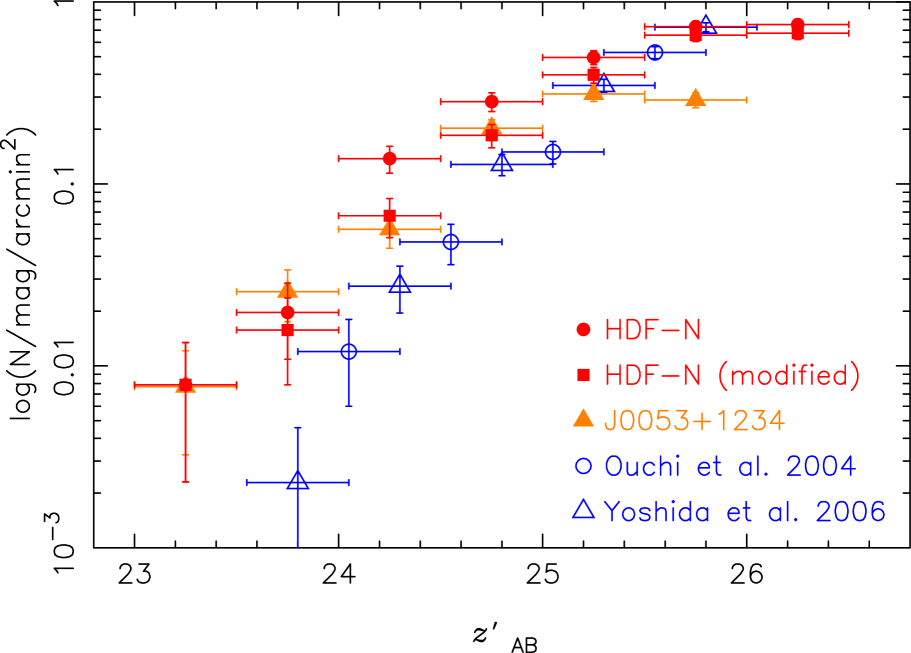
Figure 12: The $z^{\prime}$-band number count of LBGs at $z\sim 5$. Filled circles and triangles are those for the HDF-N and J0053+1234 regions, respectively, based on the sample selected using our colour criteria. Number counts of $V$-drop LBGs in SDF are shown with open circles (Ouchi et al., 2004a) and open triangles (Yoshida et al., 2006). Filled squares show the number counts of LBGs in the HDF-N selected using the modified colour criteria based on those used in Ouchi et al.(2004). See text for details. No correction for incompleteness has been made. Vertical error bars show simple Poisson errors.

In addition to the change in the number density of objects, the change of colour selection criteria reduces the effective volume. These two effects counteract each other and, as a result, the luminosity function would remain relatively unchanged. Because of the difference in the filter sets, we cannot calculate the effective volume in the case of applying the colour selection criteria of Ouchi et al. (2004a) to our sample. We are thus unable to calculate the UVLF with such criteria and so must remain focused on comparing raw number counts. However, as we have mentioned in section 4.1, slight changes to the colour selection criteria do not change the shape of the UVLF.

Although the number of objects in our sample which were observed with optical spectroscopy is still limited, 6 out of 8 objects with $z^{\prime}$-band magnitude between 24.0 and 24.5 mag in the HDF-N region for which we obtained spectroscopy are confirmed to be at $z>4.5$ (including one AGN; Ando et al. 2004). The redshifts of the remaining two objects are unidentified due to the absence of clear spectral features. Thus, we believe that most of bright objects in our sample are genuine LBGs at $z\sim 5$. Indeed, if the success rate of spectroscopic confirmation (6/8) for bright LBGs is representative of that for the whole of our sample, it implies that at least 26 among the 35 HDF-N-region galaxies with $z^{\prime}=24.0$–24.5 are at $z>4.5$. This number density of 26/505.85=0.051 arcmin^-2 well exceeds the number density of candidates in the same magnitude range (12/875=0.013 N/arcmin^-2) in Yoshida et al. (2006). Consequently, it is possible that Ouchi et al. (2004a) and Yoshida et al. (2006) may miss significant numbers of luminous high-$z$ objects unless the field-to-field variance between the HDF-N region and SDF is far larger than expected. However, such large field-to-field variance seems unrealistic considering the spatial distribution of LBG candidates in our survey fields and the similarity of the UVLF results in our two fields.

Thus, although the cause of this discrepancy remains an open question, because of the comparisons and considerations described above, we think our UVLF is robust. Hereafter we use our final LF result as a representative $z\sim 5$ UVLF to compare with UVLFs at lower redshift ranges.

4.4 Comparisons with results of numerical simulations

Recent development of computer resources and numerical techniques makes comparisons of observational results with results from numerical simulations interesting since such comparisons make it possible to investigate the physics behind the observed properties of galaxies. Night et al. (2006) executed cosmological SPH simulations, calculated SEDs for galaxies in their simulations using the population synthesis code of Bruzual and Charlot (2003), and then applied LBG colour selection criteria to create a simulated sample of LBGs at $z=$4–6. They use this sample to compare UVLFs in their numerical simulations with ours (UVLF for the HDF-N region) and with Ouchi et al. (2004a). Since the prescriptions of Night et al. (2006) do not include attenuation by dust, their UVLFs can be shifted along the luminosity axis by varying the assumed amount of uniform dust attenuation. The UVLF of $z=5$ LBGs in their simulations can be made to agree with observed UVLFs (both ours and that by Ouchi et al. 2004a) by varying dust attenuation between $E(B-V)=0.15$ and $0.3$ (using the attenuation law by Calzetti et al. 2000). Finlator et al. (2006) applied dust attenuation based on a correlation between the metallicity and dust attenuation inferred from the large sample of nearby galaxies taken from the Sloan Digital Sky Survey. They only show galaxies at $z=4$ in their numerical simulations, and their UVLF is broadly consistent with observational results at $z\sim 4$ such as Sawicki and Thompson (2006a), Ouchi et al. (2004a) and Gabasch et al. (2004a). Although the UVLFs found in numerical simulations by Night et al. (2006) and Finlator et al. (2006) show fairly steep slopes, $\alpha\ga-1.7$, such slopes are estimated from magnitude ranges fainter than the limiting magnitudes of current deep observations ($m\ga 27$). Thus, in summary, no serious conflict with observed results has been found in these numerical simulations. However, we should note that there are free parameters in models used in these simulations which are not strongly constrained by physics in a self-consistent way (e.g., amount of dust attenuation, effects of feedback from star formation and AGN), and it is still not possible to discriminate the “best” observed UVLF through the comparisons with results of such numerical simulations. One interesting prediction common in these two simulations is that UV-luminous objects should have higher stellar mass than low-luminosity ones. This trend may be related to the differential evolution of galaxies we describe in section 5, and this prediction is testable with deep infrared observations of LBGs at $z\ga 4$.

5 Differential Evolution of UV Luminosity Function from $z\sim 5$ to 3

5.1 Comparison with the $z\sim 4$ and 3 UVLFs by Sawicki and Thompson (2006)

Sawicki and Thompson (2005; 2006a) constructed ultra-deep samples of UV-selected star-forming galaxies at $1.7<z<4$ using the very same $U_{n}G{\cal R}I$ filters and colour selection criteria as those used at brighter magnitudes by Steidel and his collaborators. Using these very deep samples, Sawicki and Thompson (2006a) derived the UVLFs reaching far below $L^{*}_{z=3}$. Specifically, at $z=3$ their limiting magnitude is $M_{lim}\sim-18.5$ mag and $M_{lim}$ is about $-19.0$ mag at $z\sim 4$. These depths are about 1.5 magnitudes fainter than previous large-area studies (e.g., Steidel et al. 1999), but the results are highly reliable because of the use of the selection technique identical (down to the same filter set and color-color selection criteria) to that in the Steidel et al. work. Comparisons of our new $z\sim 5$ UVLFs with these deep UVLFs at lower redshifts can lead to crucial insights regarding the evolution of UV-selected star-forming galaxies during early epochs in the history of galaxy formation.

In Fig. 13 we show our new $z\sim 5$ UVLF (the final weight-averaged LF, as described in sec. 4.2) along with the $z\sim 4$ and $z\sim 3$ UVLFs from Sawicki and Thompson (2006a). In I03 we compared the previous, shallower version of our $z\sim 5$ UVLFs with $z=3$–4 UVLFs by Steidel et al. (1999) and argued that there is no significant difference between UVLFs from $z=3$ to 5, although there might be a slight decrease in the fainter part. This suggested trend now becomes clear thanks to the availability of deeper galaxy samples at all three epochs: although the limiting absolute magnitude of our $z\sim 5$ sample is shallower than the lower-$z$ samples of Sawicki and Thompson (2006a), we see that at luminosities fainter than $L^{\ast}_{\mathrm{z=3}}$ ($M_{\mathrm{UV}}\approx-21.0$) the number density of LBGs steadily increases from $z=5$ to 3, while no number density evolution is found at brighter magnitudes.

In order to be rigorous we need to quantify the strength and statistical significance of this differential, luminosity-dependent evolution. However, we do not wish to compare the evolution of the Schechter function parameters because the three Schechter parameters ($M^{*}$, $\phi^{*}$, and $\alpha$) are highly degenerate and so it is difficult to physically interpret the meaning of their time-evolution. Instead, it would be far better to study the evolution of the observed number densities directly, but this is not simple since, at the three different epochs, the UVLF data span somewhat different luminosity ranges, and because the magnitude bins are centred at different $M_{\mathrm{UV}}$. To overcome these problems, we use the approach developed by Sawicki and Thompson (2006a) — we investigate how far the observed number densities at the three epochs deviate from a fiducial model, for which we adopt the Schechter function fit to their $z\sim 3$ data. In this way, for each data point, we construct $\Phi(M,z)=\phi_{data}(M,z)/\phi_{fit}^{z\sim 3}(M)$, which measure the departure of the data from the model. At $z\sim 3$, $\Phi(M)\sim 1$ at all $M$, reflecting the fact that the $z\sim 3$ Schechter function is a good description of the $z\sim 3$ data. At other redshifts, however, the $\Phi(M)$ deviate from unity, reflecting the UVLF’s evolution. Next, at each epoch we compute $\bar{\Phi}(z)$ — i.e., the average of the $\Phi(M,z)$ — for bins brighter (and fainter) than $M_{UV}=M^{*}_{z=3}=-21.0$ mag. Finally, the ratio of the $\bar{\Phi}$ at two redshifts tells us the amount of number density evolution that a given population (bright or faint) undergoes.

The results of the above procedure are shown in Fig. 14 (see also Table 9), which shows the number density evolution of the bright end (horizontal axis) and the faint end (vertical axis) of the UVLF. The data show strong evidence for evolution of the faint end of the UVLF: at $z\sim 5$ there are only 0.34 $\pm$ 0.02 as many faint galaxies as there are at $z\sim 3$. This represents a three-fold increase that is highly statistically significant. The evolution over $z\sim 5\rightarrow 4$ is smaller (it is a 1/0.78 = 1.3-fold increase), but since the cosmic time between $z=4.8$ and $z=4$ ($\sim$300 Myr) is half of the interval between $z=4$ and $z=3$ ($\sim$600 Myr), the data are completely consistent with the idea that the number of faint LBGs increases at a constant rate from $z\sim 5$ to 3. However, while the faint end of the UVLF is evolving, there is no evidence for any change in the number density of luminous ($M_{\mathrm{UV}}<-21.0$ mag) galaxies over $z\sim 5\rightarrow 4\rightarrow 3$. Indeed, the $z\sim 5\rightarrow 3$ data rule out a scenario — indicated by the diagonal line — in which the number density of galaxies evolves uniformly at all luminosities. These $z\sim$5-based results are in excellent agreement with the trends found at $z\sim 4\rightarrow 3$ by Sawicki and Thompson (2006a) (shown with green symbols), although our new $z\sim 5$ data both lengthen the cosmic time baseline and strengthen the statistical significance of those earlier conclusions.

In summary, the comparison of our UVLF at $z\sim 5$ with those at $z=3$–4 from Sawicki and Thompson (2006a) indicates that the evolution of LBG number densities depends on UV luminosity. Over the $\sim$1 Gyr from $z\sim 5$ to $z\sim 3$, the number density of luminous LBGs stays almost unchanged while there is a gradual and steady build-up in the number density of faint ($M_{\mathrm{UV}}\ga-21$ mag) galaxies.

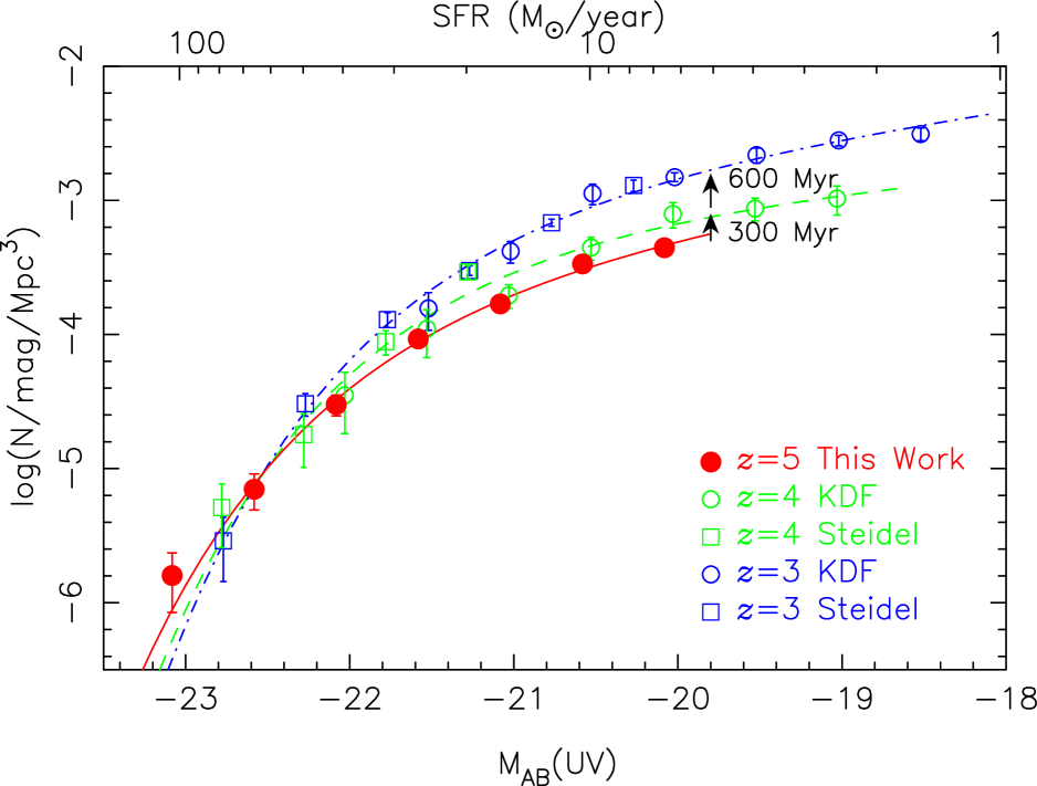
Figure 13: UV luminosity function (UVLF) at $z\sim 5$ (solid circles and solid line) in this study and those at $z\sim 4$ (dashed line) and at $z\sim 3$ (dot-dashed line) by Sawicki and Thompson (2006a).

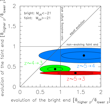
Figure 14: Luminosity-dependent evolution of the number density of galaxies. The horizontal axis shows the change in the number density of luminous galaxies ($M_{UV}<-21.0$ mag) expressed as the ratio between the normalized average densities $\bar{\Phi}$ at the redshift pairs indicated. The vertical axis shows the same quantity but for low luminosity galaxies ($M_{UV}>-21.0$ mag). The error ellipses show 68% and 95% confidence regions, while the straight lines represent three fiducial evolutionary scenarios as labelled. At $z\sim 5$ there are only $\sim 1/3$ as many faint galaxies as at $z\sim 3$, and it is clear that the evolution of the UVLF is luminosity-dependent over $z\sim 5\rightarrow 3$ and $z\sim 4\rightarrow 3$.

5.2 Implications of UV Luminosity-dependent Evolution

5.2.1 Star Formation History of LBGs

The UV luminosity-dependent evolution of UVLF has been already pointed out by Sawicki and Thompson (2006a) for their LBG samples at $z\sim 3$ and 4. Our data indicate that similar evolutionary trends were already in place at earlier cosmic times.

Sawicki and Thompson (2006a) discuss three possible scenarios responsible for the differential evolution of the UVLF between $z\sim 4$ and 3. The first one is the straightforward increase of the number of low-luminosity LBGs at later epochs. They argue that, if the ages of low-luminosity LBGs at $z\sim 3$ are mostly smaller than 600 Myr, the increase in number density can be a natural consequence of the emergence of large population of low-luminosity galaxies after $z\sim 4$. Sufficiently young ages of $z\sim 3$ LBGs have been suggested by several authors. For example, Shapley et al. (2001) used rest-frame UV to optical SEDs of their (fairly bright) sample LBGs for comparisons with template SEDs based on models with a simple constant star formation history and derived a median age of 320 Myr, and results with similar or younger age estimates have been also reported by other authors (e.g., Sawicki and Yee 1998; Papovich et al. 2001; Iwata et al. 2005). We should note, however, that the ages estimated by SED fitting based on simple star formation history models (constant or exponentially decaying SFH) are strongly affected by recent star formation activity. Thus the age should be interpreted as time since the onset of most recent star formation, and such age estimates may be incorrect if LBGs have sporadic star formation histories. As we have discussed in I03 , since the number density of LBGs in the luminous part of the UVLF shows little change from $z\sim 5$ to 3, the small ages of LBGs at $z\sim 3$ would imply that the star formation histories of LBGs are sporadic, and that individual LBGs would have experienced short bursts of star formation during their evolution. Thus, if the evolution of the fainter part of the UVLF represents the emergence of a large population of low-luminosity LBGs at later epochs, it should be interpreted as the increase in the number density of low-luminosity population as a whole, and for individual galaxies a low-luminosity LBG at $z\sim 4$ can be a luminous one at $z\sim 3$ and vice versa.

The change in the properties of starbursts, such as intensity, duration and duty cycles, can be the second possible cause of differential evolution. It would be possible to explain the increase in the number density of faint galaxies by introducing the differential change in the properties of starburst depending on UV luminosity (scenario B of Sawicki and Thompson 2006a). If intrinsically less luminous galaxies (unexplored with current observations when in their low star formation state) progressively spend longer time in the relatively luminous phase, they can be observable by $z\sim 3$, and as a consequence the number density in the faint end of the UVLF could increase. The luminous end would not change if the starburst properties of luminous galaxies remain the same. Such scenario might be tested through the comparison of starburst ages of LBG populations at different epochs. Exploration of the stellar populations of LBGs at $z\ga 4$ has become possible recently thanks to the availability of rest-frame optical data obtained through mid-infrared imaging with the Spitzer space telescope, and several authors have reported the existence of massive galaxies at $z\sim 6$ (e.g., Eyles et al. 2005; Mobasher et al. 2005; Yan et al. 2006). Measurement of stellar masses would to some extent resolve the ambiguity for the star formation history of LBGs present in analyses based solely on the rest-frame UV wavelengths. A systematic study based on a uniform selection scheme across the redshift range $z=3$–5 would be an interesting project to pursue in order to address these issues.

One of the major obstacles for precise estimation of LBGs’ ages would be the notorious degeneracy between age and dust in their effects on galaxy SEDs. Indeed, Sawicki and Thompson (2006a) raised the change of dust properties as the third possible cause of differential evolution. If the property of dust changes differentially depending on UV luminosity, this would also alter the shape of the UV luminosity function. Unfortunately, we know quite little about the properties of dust in high-z star-forming galaxies, and usually one attenuation law (such as Calzetti et al. 2000) is assumed for all galaxies in a high-$z$ sample. Thus, it could be difficult to discriminate whether it is age or dust that changes by studying the discrete SEDs obtained through the broad-band imaging data.

5.2.2 Biased Galaxy Evolution

We recently found that Lyman $\alpha$ equivalent widths of $z\sim 5$–6 LBGs (and Lyman $\alpha$ emitters) tend to depend on UV luminosity (Ando et al., 2006): high luminosity LBGs show little or no Lyman $\alpha$ emission, while there are objects with $M_{\mathrm{UV}}>-21$ mag which show strong emission lines. Along with the result presented in this paper that the number density of luminous LBGs at $z\sim 5$ is almost the same as at later epochs, the UV luminosity dependence of Lyman $\alpha$ equivalent widths is another indication that UV luminous galaxies have different properties from fainter ones. As discussed in Ando et al. (2006), there are several possible causes of the luminosity dependence of the strength of Lyman $\alpha$ emission, one possible explanation being that luminous LBGs are embedded in dense reservoirs of neutral hydrogen gas. The existence of such large reservoirs of neutral gas could be the cause of the large star formation rates we see and also could be the underlying cause of the heavy absorption of Lyman $\alpha$ emission by ionized gas surrounding the star forming regions within galaxies. Another possibility is the large amount of dust and/or metals in UV-luminous LBGs which have experienced significant amounts of star formation until $z\sim 5$. The existence of strong silicon and carbon interstellar absorption lines (Ando et al., 2004) in the luminous objects in our sample of $z\sim 5$ LBGs supports this idea, although sample size is still quite limited. A third indication of the UV luminosity dependence is the relatively small number of bright objects with blue rest-frame UV colours in our sample (section 3.6 and Fig. 5). The dependence on UV luminosity of the clustering strength of $z=3$–5 LBGs has also been reported by several authors (e.g., Giavalisco and Dickinson 2001; Ouchi et al. 2004b; Kashikawa et al. 2006). It suggests UV luminous LBGs reside in relatively massive dark matter haloes.

The existence of a number density of UV luminous LBGs at $z\sim 5$ that is comparable to those at $z=3$–4, as well as the luminosity-dependent properties of LBGs especially at $z\sim 5$, support the idea of biased galaxy formation. The luminous galaxies, presumably hosted by relatively massive dark matter haloes which are also reservoirs of huge amounts of neutral gas, might start bursts of star formation at early epochs (i.e., $z>5$). On the other hand, the number density of faint objects ($M_{\mathrm{UV}}>-21$ mag) gradually increases along with the increase in the number density of dark matter haloes. The UV luminous objects, which have SFRs as large as $100M_{\sun}$/yr^-1 at $z\sim 5$, may become fainter at later times because the duration of such enormous bursts of star formation can be on order of 100 Myr at most given that significantly longer bursts would result in masses that exceed $10^{11}M_{\sun}$ by $z\sim 3$. However, some fraction of objects that are relatively faint at $z\sim 5$ would be ignited during the period between $z\sim 5$ and 3, and this would make it possible to keep the number density of UV-luminous LBGs as a whole almost constant over the intervening $\sim$1 Gyr. Such mixing of LBG populations that represent different generations across cosmic time may by $z\sim 3$ extinguish the dependence of dust / metal or of gas mass on UV luminosity, and this mixing may explain the apparent absence of UV luminosity dependence of Lyman $\alpha$ equivalent widths and strengths of interstellar metal absorption lines at these lower redshifts(Shapley et al., 2003). This biased formation hypothesis could be tested by further analyses of chemical compositions and stellar populations for LBGs at different redshifts and luminosity ranges. Although attempts to tackle these issues have been started (e.g, Ando et al. 2004; Eyles et al. 2005; Labbé et al. 2007), deep follow-up observations in both spectroscopy and multi-wavelength imaging that cover many sample galaxies are required.

5.3 Comparison with UVLFs at $z\ga 6$

Recently, there have been several attempts to determine the UVLF at $z\sim 6$ through deep observations in $i$ and $z$ bands (e.g., Bouwens et al. 2003; Bunker et al. 2004; Yan and Windhorst 2004; Shimasaku et al. 2005). Bouwens et al. (2006) made a compilation of very deep observations with HST (GOODS-N, GOODS-S, the Hubble Ultra Deep Field (UDF) and UDF pararell ACS fields) and derived the $z\sim 6$ UVLF at $1350\AA$ down to $M_{1350}\sim-17.5$ mag. They argued that there is a strong evolution in the number density of luminous ($M<-21$ mag) LBGs from $z\sim 6$ to $z\sim 3$, while the number density of faint galaxies is comparable to or even larger than that at $z\sim 3$. They claim that it could be caused by the brightening of $M^{\ast}$ along cosmic time. Also, Bouwens and Illingeorth (2006) utilized deep HST/NICMOS observations to find LBGs at $z\approx 7$–8 and concluded that there is a deficiency of luminous galaxies at $z\approx 7$–8 compared to $z\sim 6$, suggesting that the rapid evolution of the number density of luminous galaxies has started at $z\ga 7$. Their arguments are opposite from the differential evolution of UVLFs we found for the redshift range 3–5, and these two sets of results would be inconsistent if one assumes that the number density evolution from $z\sim 6$ to 3 proceeds continuously. However, we should note that the number densities in the fainter part of the $z\sim 6$ UVLF reported by several authors have a fairly large scatter (see Table 13 and Figure 14 in Bouwens et al. 2006 for a summary), even though most of these studies are based on similar data sets taken from deep HST surveys. Also, current deep HST based studies for $z\sim 6$ LBGs suffer from severe limitations in survey volumes. The GOODS survey area which Bouwens et al. (2006) relied on to correct for the field-to-field variations is just a fourth of the effective survey area presented here. Thus the $z\sim 6$ UVLF and its Schechter parameters would be still need to be further examined. Although the number of objects with $z_{850}<25.5$ mag (which roughly corresponds to $M^{\ast}_{\mathrm{z=3}}$) detected in the GOODS area by Bouwens et al. (2006) (8 objects) is inconsistent with no evolution from $z\sim 5$ even considering the dimming from $z\sim 5$ to 6 and the difference in the rest-frame wavelength traced by the $z$-band filter (which may lead to $\sim 0.1$ mag of dimming), it is still premature to draw a conclusion that whether the UVLF evolution from $z\sim 6$ to 3 is due to the brightening of $L^{\ast}$. Further studies of $z\sim 6$ LBGs, especially those based on wider survey area are indispensable (cf. Shimasaku et al. 2005).

6 UV Luminosity Density

6.1 UV Luminosity Density at $z\sim 5$

Using the updated luminosity function of $z\sim 5$ LBGs we can calculate the UV luminosity density at that epoch more reliably than we did in I03 thanks to the deeper and wider data. The luminosity density at a target epoch due to light emitted from galaxies brighter than $L_{lim}$ can be calculated by the integration of the LF as

$$\rho(L>L_{lim})=\int^{\infty}_{L_{lim}}L\phi(L)dL.$$

We take two ranges of integration. One lower limit in the integration is $M_{\mathrm{UV}}\leq-18.5$, which corresponds to $0.1L^{\ast}_{\mathrm{z=3}}$, and the other is $L_{lim}=0$. The formal lower luminosity limit has been used by several previous studies (e.g., Steidel et al. 1999; Sawicki and Thompson 2006b; Bunker et al. 2006), and corresponds to the limiting magnitude of the $z\sim 3$ LBG sample of Sawicki and Thompson (2006a). At $z\sim 5$, we have to extrapolate our observed UVLF more than 1 magnitude in order to obtain the UV luminosity density integrated down to $M_{\mathrm{UV}}\leq-18.5$ mag. With the extrapolation of the integral down to zero luminosity ($L_{lim}=0$) we want to estimate the total UV luminosity density emitted from star-formation galaxies into inter-galactic space. By comparing the UV luminosity densities down to $0.1L^{\ast}_{\mathrm{z=3}}$ with the total ones we are able to estimate the contribution from faint objects. The steepness of the UVLF faint-end slope has a crucial importance for the total UV luminosity. As we have stated in section 4.2, the faint-end slope of the UVLFs is still not well constrained by observations (especially for higher redshift, i.e., $z>4$), and it introduces a large uncertainty in the estimation of total UV luminosity density.

Fig. 15 shows with filled circles the UV luminosity densities obtained from our data at $z=4.8$. The integrations are made using the best-fit Schechter function for the final UVLF described in section 4.2, and error bars indicate $1\sigma$ errors calculated using Schechter functions for perturbed data generated to obtain 68% confidence parameter ranges (see section 4.2). Table 10 lists the UV luminosity densities at $z\sim 5$ calculated using the final UVLF and the UVLF for the HDF-N region. Our survey only reaches to $M_{\mathrm{UV}}<-19.8$, and thus 68% (49%) of UV luminosity density integrated down to $M_{\mathrm{UV}}\leq-18.5$ ($L_{lim}=0$) comes from this observed luminosity range. Since our updated UVLF presented here is consistent with our previous (I03 ) one in the luminosity range covered by the previous data, the UV luminosity density at $z\sim 5$ also shows little change from the value in I03 .

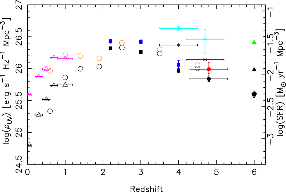
Figure 15: UV luminosity densities at various redshifts. Coloured symbols: UV luminosity densities integrated down to zero luminosity. Black-and-white symbols: UV luminosity densities integrated down to $L_{\mathrm{U}V}=0.1L^{\ast}_{z=3}$ ($M_{\mathrm{U}V}=-18.5$ mag). Filled circles at $z=4.8$: this work, using the UVLF derived from the combination of our two survey fields. Open triangles at $0<z\leq 1$: based on UVLFs by Takeuchi et al. (2005). Filled squares at $2.2<z<4$: Sawicki and Thompson (2006b). Crosses at $z=4.0$ and $z=4.7$: Ouchi et al. (2004). Filled triangles at $z=6$: Bouwens et al. (2006). Pentagon at $z=6$: Bunker et al. (2006). Open circles: Gabasch et al. (2004). For published data points error bars are shown only when authors provide error values for UV luminosity density at these specific integration ranges ($L_{\mathrm{U}V}\ga 0.1L^{\ast}_{z=3}$ and $L>0$). The right vertical axis indicates the comoving star formation density converted from UV luminosity density. The conversion factor in the logarithmic scale is 27.903 (Madau et al. 1998).

6.2 Evolution of UV Luminosity Density

In Fig. 15 we also show results for various redshifts by other authors. For $z\leq 1$, we show UV luminosity density data from the combined sample of GALEX and VIMOS-VLT Deep survey (Takeuchi et al. 2005, who took the UVLF data from Arnouts et al. 2005). The UV luminosity densities at $z\sim 2$, 3 and 4 are from Sawicki and Thompson (2006b). Their results are based on UVLFs in Sawicki and Thompson (2006a). Redshift 4.0 and 4.7 results by Ouchi et al. (2004a) are also shown. At redshift 6 we show results by two different authors: triangles are from Bouwens et al. (2006) and the pentagon is from Bunker et al. (2006) (only the value for $L\geq 0.1L^{\ast}_{\mathrm{z=3}}$ is provided in the latter paper). The rest-frame wavelengths of all of these observations lie within 1350Å–1700Å. For these published values, we only show error bars when errors for these specific integration ranges ($L\geq 0.1L^{\ast}_{\mathrm{z=3}}$ and $L>0$) are provided in the papers, since we do not know the range of Schechter LF parameters for $1\sigma$ confidence level which is required to precisely calculate luminosity density error values. No extinction correction has been applied.

In the redshift range $z\ga 4$ the data points show fairly large discrepancies. As has been pointed out in Sawicki and Thompson (2006b), the value obtained by the SDF for $z\sim 4$ is about 2.5 times larger than that by the KDF for the integration down to $L=0.1L^{\ast}_{\mathrm{z=3}}$ and the disagreement reaches a factor of 3.7 when extrapolated to zero luminosity. The situation is similar at $z\sim 5$ where SDF estimates of UV luminosity density are larger than our results by factors of 2–3. The large luminosity density values by Ouchi et al. (2004a) come from relatively large number densities in the fainter part of their UVLF (see Fig. 9 of Sawicki and Thompson 2006a). By unconstrained Schechter function fitting they obtained the best-fitted faint end slope of $\alpha=-2.2$ for $z\sim 4$ LBGs, which is significantly steeper than the one by Sawicki and Thompson (2006a) ($-1.26$) and the values estimated for $z\sim 3$ LBGs ($\approx-1.6$ to $-1.4$; Steidel et al. 1999; Sawicki and Thompson 2006a). In addition to UV luminosity density estimates based on this steep $\alpha=-2.2$ slope, they also examined cases with a fixed UVLF slope value of $-1.6$ to calculate UV luminosity densities at $z=4$–5, and all results from Ouchi et al. (2004a) shown in Fig. 15 are based on calculations assuming the faint end slope fixed to $-1.6$.

The Ouchi et al. (2004a) $z\sim 5$ number density at $M_{\mathrm{UV}}\approx-20.8$ mag (the faintest data point for them) is comparable to ours, but since their brighter part of the UVLF has smaller number densities than does our LF, their best-fitted $M^{\ast}$ is fainter and $\phi^{\ast}$ is larger than ours. Their assumed faint-end slope ($-1.6$) is also steeper than our best-fit value ($-1.48$). As a result, the contribution from fainter objects (extrapolated beyond the observed limiting magnitude) to the UV luminosity becomes larger than that in our data. The large differences between the Ouchi et al. (2004a) total UV luminosity densities and those integrated down to $0.1L^{\ast}_{\mathrm{z=3}}$, at both $z\sim 4$ and $z\sim 4.7$, also indicate that in their results the UV luminosity density comes mainly from unexplored faint populations. Because the bulk of UV luminosity emitted into inter-galactic space is from galaxies with UV luminosity $L_{\mathrm{UV}}\la L^{\ast}$, luminosity ranges probed by Ouchi et al. (2004a) and I03 are too shallow to definitely measure the total UV luminosity. This is also the case for our result presented in this paper, since our data are deeper but still only reach to $0.3L^{\ast}_{\mathrm{z=3}}$. For $z\sim 6$, the studies presented here both (at least partly) use the common Hubble Ultra Deep Field (UDF) data but, despite this, their results differ from each other. To discuss in detail what causes this discrepancy at $z\sim 6$ is beyond the scope of this paper, but considering the facts that $z\sim 6$ LBGs are primarily selected by one $i-z$ colour, and that in both studies UV continuum luminosity estimated from $z^{\prime}$-band magnitudes may suffer attenuation by intergalactic neutral hydrogen, this diversity at $z\sim 6$ may be caused by the uncertainty in sample selection and/or correction for UV luminosity (cf. Sawicki and Thompson 2006b).

Despite the uncertainty in the higher redshift ranges, it would be meaningful to examine the overall change of UV luminosity density with redshift using the currently available data in order to see the cosmic evolution of star formation activity. The trend suggested by Gabasch et al. (2004b) based on their photometric redshift sample, is that at $z\ga 3$ the UV luminosity density is slowly declining with increasing redshift. This trend is consistent with the combination of Sawicki and Thompson (2006a) and our results, and the UV luminosity density values of Gabasch et al. (2004b), determined from the UVLF for galaxies with photometric redshift $4<z<5$, also agree reasonably well with ours results. If we restrict ourselves to see only data points with integration down to $0.1L^{\ast}_{\mathrm{z=3}}$ (black and white points in Fig. 15), which are less affected by the uncertainty of the UVLF faint-end slope, then all the data in Fig. 15 show a consistent picture that the UV luminosity density (i.e., comoving star formation density, if we neglect the effect of dust attenuation) is low at $z\sim 6$ (when the cosmic age is $\approx 0.9$ Gyr) and gradually increases until $z\sim 2$–3 (when the cosmic age is 2–3 Gyr). From that epoch on the UV luminosity density declines rather rapidly until now.

This overall cosmic evolution of UV luminosity density might indicate that some kind of transition in star-forming galaxies has happened at $z\approx 2-3$. At $z<2$, it has been pointed out that in the later epochs there is an absence of massive galaxies with large SFR while less massive galaxies continue to form stars. This trend is called “down-sizing” and recent development of deep and wide imaging surveys and intensive surveys using multi-object spectrographs (e.g., Kodama et al. 2004; Treu et al. 2005; Juneau et al. 2005; Pérez-González et al. 2005) made this trend clearer than when it was first suggested (Cowie et al., 1996). On the other hand, in this paper we have argued that there is differential galaxy evolution at $z\ga 3$, i.e., that the galaxy population with high SFRs maintains its number density from early times, $z\sim 5$, until $z\sim 3$, while the number density of galaxies with smaller SFRs gradually increases. Moreover, we also discussed that this differential evolution could be an indication of biased galaxy evolution in the early universe. The break in the UV luminosity density around $z\approx$2–3 may indicate the transition from biased galaxy evolution to down-sizing. In other words, the formation of massive galaxies, i.e., the active assembly of stellar mass within the massive dark matter haloes, might have started at $z>6$ and continued at roughly constant rate for more than 2 Gyr, with the bulk of stellar mass assembly in such massive haloes terminating around $z\sim 2$. Although the observational evidence of down sizing has accumulated rapidly, the biased galaxy evolution at higher redshift is still just a hypothesis. Moreover, currently we only deal with rest-frame UV properties which are dominated by the effects of short time-scale starbursts. In order to investigate what is happening at $z>3$ and to relate that activity to down-sizing in the lower redshift range, we need information on masses (either stellar or of dark matter haloes).

6.3 Contribution to the Ionizing Background Radiation

UV luminosity density can be used to estimate the contribution of stellar sources to the cosmic ionizing background radiation under an assumption about the ratio of ionizing radiation flux escaping from galaxies to non-ionizing UV radiation. In I03 we argued that if the escape fraction is as large as 0.5, then ionizing radiation from star-forming galaxies and from QSOs at $z\sim 5$ may be sufficient to keep the universe at that redshift ionized. Several studies of galaxies at $z\sim 6$ have discussed whether the UV luminosity density of $z\sim 6$ galaxies is sufficient to keep the universe ionized (e.g., Bouwens et al. 2003; Bouwens et al. 2006; Yan and Windhorst 2004; Bunker et al. 2006). However, since the escape fraction of ionizing photons from galaxies is still almost unknown observationally (e.g, Steidel et al. 2001; Giallongo et al. 2002; Inoue et al. 2005; Shapley et al. 2006), such arguments cannot be definitive. Additionally, the uncertainty in the UVLF, especially in its faint-end slope, makes the estimates of ionizing radiation difficult. On the other hand, Inoue et al. (2006) used the evolution of the UV luminosity density presented in Fig. 15, emission from QSOs, IGM opacity model and ionizing background radiation in the redshift range 0 to 6 to predict the escape fraction of star-forming galaxies. They found that evolution of the escape fraction — i.e., higher ($\ga 0.2$) escape fraction at higher redshift ($z\geq 4$) — may be required. Unfortunately, the direct observation of ionizing radiation at $z\ga 4$ is extremely difficult due to the increasing opacity of the IGM. We should first investigate the properties of ionizing radiation from galaxies at $z\la 3$ to know the typical value of the escape fraction in the high-redshift universe and its relation to other physical properties of galaxies.

7 Summary and Conclusions

In this paper we have reported the construction of a large sample of Lyman break galaxies (LBGs) at $z\sim 5$ and their UV luminosity function (LF), obtained from deep large-area Subaru observations in two blank fields, namely, the Hubble Deep Field-North and the J0053+1234 regions. Our main findings are as follows:

• Over an effective survey area of 1290 arcmin², we obtained 853 LBG candidates at $z\sim 5$ with $z^{\prime}<26.5$ mag. Spectroscopic redshift data for galaxies at lower redshifts ($z<4$) from published redshift surveys in the target fields as well as the results of follow-up spectroscopy for a subset of our LBG candidates confirm that our colour selection criteria are defined so that star-forming galaxies at $z\sim 5$ are efficiently selected and contaminations from objects at lower redshift are properly eliminated.

• In the bright end of the UVLF there is no significant change in the number density from $z\sim 5$ to 3, while we found a gradual increase from $z\sim 5$ to 3 in the LF’s fainter part ($M_{\mathrm{UV}}>-21$ mag). Such differential evolution of the UVLF from $z\sim 4$ to 3 has been pointed out by Sawicki and Thompson (2006a), and our present work shows that this trend was already underway at earlier cosmic times.

• We found a deficiency of galaxies with blue UV colours ($I_{c}-z^{\prime}<0$) at bright magnitudes ($z^{\prime}\la 24.5$ mag). This trend is significant even if we take photometric errors into account.

• The UV luminosity density at $z\sim 5$, calculated by integrating the UVLF, is found to be $38.8^{+6.7}_{-4.1}$% of that at $z\sim 3$, for the luminosity range $L>0.1L^{\ast}_{\mathrm{z=3}}$. By combining our results with those from the literature, we found that the cosmic UV luminosity density is slowly increasing with cosmic age from $z\sim 6$, that it then marks its peak at $z=3$–2, and then declines until the current epoch.

We have discussed the origins of the differential evolution of the UVLF along cosmic time and suggested that our observational findings are consistent with the biased galaxy evolution scenario. A galaxy population hosted by massive dark haloes starts active star formation preferentially at early times and maintains its activity until $z\sim 3$, while less massive galaxies increase their number density later. This idea is supported by other observational findings, including, (1) the deficiency of UV luminous objects with blue UV colours, (2) the fact that UV luminous objects at $z\sim 5$ have smaller Lyman $\alpha$ equivalent widths compared to fainter objects, and (3) the dependence of clustering strengths on UV luminosity which suggests that UV luminous objects are more likely to be hosted by massive dark matter haloes. Further investigations of the properties of LBGs, especially at higher redshifts ($z>4$) and with wider dynamic ranges in luminosity and wavelength, are required to test the reality of the biased galaxy evolution scenario.

Table 1: A summary of observations for HDF-N. Limiting magnitude is for 5 $\sigma$ with 1.2″diameter aperture.

Filter	Single Exposure Time	Number of shots	Total integration time	Limiting mag.	Seeing
	sec		sec		″
$V$	720–1,440	14	24,720	28.17	1.11
	600	10
$I_{c}$	180–300	11	6,180	26.86	1.13
	360–420	10
$z^{\prime}$	120–215	21	11,935	26.55	1.13
	180–280	41

Table 2: A summary of observations for J0053+1234. Limiting magnitude is for 5 $\sigma$ with 1.2″diameter aperture.

Filter	Single Exposure Time	Number of shots	Total integration time	Limiting mag.	Seeing
	sec		sec		″
$V$	600	23	13,800	27.79	0.89
$I_{c}$	200	10	2,000	26.39	0.87
$z^{\prime}$	240	28	6,720	26.24	0.88

Table 3: Cross identifications of objects with previously published spectroscopic redshifts at $4.5<z<5.5$ in the HDF-N region.

ID	R.A.(J2000)a	Dec.(J2000)a	$z^{\prime}$ mag.	$V-I_{c}$	$I_{c}-z^{\prime}$	Redshift	Ref.b
F36219-1516	12:36:21.88	+62:15:17.0	25.39	0.67	0.09	4.890	1
F36279-1750	12:36:27.74	+62:17:47.8	26.05	$>$2.32	$-0.11$	4.938	1
F36376-1453	12:36:37.62	+62:14:53.8	21.97	3.25	0.78	4.886	1
HDF 4-439.0	12:36:43.84	+62:12:41.7	25.29	1.48	$-0.19$	4.54	2
HDF 4-625.0	12:36:44.65	+62:11:50.7	25.24	$>$2.87	0.03	4.580	3
GOODS J123647.96+620941.7	12:36:47.93	+62:09:41.7	24.32	$>$3.31	$-0.10$	5.186	4
ES 1	12:36:49.23	+62:15:38.8	25.48	$>$2.96	$-0.16$	5.190	5
HDF 3-0951.0	12:37:00.23	+62:12:19.8	24.69	1.82	0.22	5.34	6
095819(A04-4)	12:37:05.68	+62:07:43.3	24.50	2.26	0.15	4.650	7
GOODS J123721.03+621502.1	12:37:21.00	+62:15:02.1	23.32	2.36	0.56	4.761	8
144200(A04-2)	12:37:57.49	+62:17:19.0	24.08	2.40	0.07	4.695	7
129178(A04-7)	12:38:04.36	+62:14:19.7	24.29	$>$3.28	0.21	5.183	7
104268(A04-1)	12:38:11.32	+62:09:19.4	24.02	2.22	0.11	4.517	7
148198(A04-8)	12:38:16.63	+62:18:05.3	24.50	$>$3.19	0.42	4.615	7
149472(A04-6)	12:38:25.52	+62:18:19.7	24.87	$>$3.02	0.14	4.857	7
139294(A04-5)	12:38:28.96	+62:16:18.8	24.39	1.96	0.20	4.667	7

^a Positions are based on our astrometry with Suprime-Cam images, using USNO-B1 catalog (see section 3.2).

^b 1: Dawson et al. (2001), 2: Stern and Spinrad (1999), 3: Fernández-Soto et al. (1999), 4: Barger et al. (2002), 5: Dawson et al. (2002), 6: Spinrad et al. (1998), 7: Ando et al. (2004), 8: Cowie et al. (2004).

Table 4: Cross identifications of objects with previously published spectroscopic redshifts at $4.5<z<5.5$ in the J0053+1234 region.

ID	R.A.(J2000)a	Dec.(J2000)a	$z^{\prime}$ mag.	$V-I_{c}$	$I_{c}-z^{\prime}$	Redshift	Ref.b
106426(A07-1)	00:52:21.34	+12:32:35.3	24.07	2.59	0.23	4.797	1
093014(A07-4)	00:52:37.37	+12:29:58.7	25.26	$>$1.85	0.16	4.491	1
091813(A07-3)	00:52:39.88	+12:29:44.1	25.03	1.98	0.06	4.391	1
104115(A07-2)	00:52:43.27	+12:32:08.2	24.22	1.75	0.16	4.267	1
CDFa G01	00:53:33.21	+12:32:07.3	23.54	2.88	0.03	4.815	2
CDFa GD07	00:53:35.57	+12:31:44.1	23.72	1.67	0.17	4.605	2
CDFb G05	00:53:51.28	+12:24:21.3	24.31	2.70	0.29	4.486	2

^a Positions are based on our astrometry with Suprime-Cam images, using USNO-B1 catalog (see section 3.2).

^b 1: Ando et al. (2007), 2: Steidel et al. (1999).

Table 5: Number of LBG candidates and UV luminosity function of LBGs at $z\sim 5$ for HDF-N.

$z^{\prime}$ mag	abs. mag	Num	$V_{\mathrm{eff}}$	$\mathrm{N_{int}}$	$\phi$(m)
			Mpc-3		N/Mpc-3/mag
23.0 – 23.5	$-$23.082	2	$3.07\times 10^{3}$	0.79	$1.55\pm 0.85\times 10^{-6}$
23.5 – 24.0	$-$22.582	5	$2.86\times 10^{3}$	2.79	$3.04\pm 0.91\times 10^{-6}$
24.0 – 24.5	$-$22.082	35	$2.68\times 10^{3}$	6.06	$4.25\pm 0.66\times 10^{-5}$
24.5 – 25.0	$-$21.582	72	$2.48\times 10^{3}$	12.58	$9.42\pm 1.05\times 10^{-5}$
25.0 – 25.5	$-$21.082	126	$2.24\times 10^{3}$	24.94	$1.78\pm 0.15\times 10^{-4}$
25.5 – 26.0	$-$20.582	186	$1.90\times 10^{3}$	24.05	$3.36\pm 0.25\times 10^{-4}$
26.0 – 26.5	$-$20.082	191	$1.51\times 10^{3}$	20.33	$4.43\pm 0.33\times 10^{-4}$

Table 6: Number of LBG candidates and UV luminosity function of LBGs at $z\sim 5$ for J0053+1234.

$z^{\prime}$ mag	abs. mag	Num	$V_{\mathrm{eff}}$	$\mathrm{N_{int}}$	$\phi$(m)
			Mpc-3		N/Mpc-3/mag
23.0 – 23.5	$-$23.082	3	$2.51\times 10^{3}$	1.40	$1.63\pm 0.69\times 10^{-6}$
23.5 – 24.0	$-$22.582	10	$2.38\times 10^{3}$	1.08	$9.61\pm 2.88\times 10^{-5}$
24.0 – 24.5	$-$22.082	22	$2.28\times 10^{3}$	2.53	$2.19\pm 0.44\times 10^{-5}$
24.5 – 25.0	$-$21.582	79	$1.99\times 10^{3}$	7.82	$9.16\pm 1.02\times 10^{-5}$
25.0 – 25.5	$-$21.082	122	$1.68\times 10^{3}$	14.85	$1.63\pm 0.15\times 10^{-4}$

Table 7: UV luminosity function of LBGs at $z\sim 5$ obtained as a weighted average of results for two survey fields. The number densities at $z^{\prime}>25.5$ come only from the HDF-N region.

$z^{\prime}$ mag	abs. mag	$\phi$(m)
		N/Mpc-3/mag
23.0 – 23.5	$-$23.082	1.60$\pm 0.75\times 10^{-6}$
23.5 – 24.0	$-$22.582	7.02$\pm 2.11\times 10^{-6}$
24.0 – 24.5	$-$22.082	3.00$\pm 0.53\times 10^{-5}$
24.5 – 25.0	$-$21.582	9.26$\pm 1.03\times 10^{-5}$
25.0 – 25.5	$-$21.082	1.69$\pm 0.15\times 10^{-4}$
25.5 – 26.0	$-$20.582	3.36$\pm 0.25\times 10^{-4}$
26.0 – 26.5	$-$20.082	4.43$\pm 0.33\times 10^{-4}$

Table 8: Schechter function parameters of UVLF at $z\sim 5$, obtained with the data from the HDF-N region only and from both the HDF-N and J0053+1234 regions.

Region	$M^{\ast}$	$\phi^{\ast}$	$\alpha$
HDF-N	$-20.82^{+0.22}_{-0.22}$	$7.7^{+1.9}_{-2.1}\times 10^{-4}$	$-1.05^{+0.35}_{-0.32}$
HDF-N and J0053+1234	$-21.28^{+0.38}_{-0.38}$	$4.1^{+2.9}_{-3.0}\times 10^{-4}$	$-1.48^{+0.38}_{-0.32}$

Table 9: Evolution of the number density for galaxies brighter and fainter than $M_{UV}=-21.0$.

Epochs	bright end ($M_{UV}<-21.0$)	faint end ($M_{UV}>-21.0$)
	$\bar{\Phi}(higherz)/\bar{\Phi}(lowerz)$	$\bar{\Phi}(higherz)/\bar{\Phi}(lowerz)$
$z\sim 5\rightarrow 3$	1.37 $\pm$ 0.44	0.34 $\pm$ 0.02
$z\sim 5\rightarrow 4$	1.58 $\pm$ 0.56	0.78 $\pm$ 0.09
$z\sim 4\rightarrow 3$	0.87 $\pm$ 0.19	0.44 $\pm$ 0.05

Table 10: UV luminosity density calculated for the luminosity range $L_{\mathrm{U}V}\ga 0.1L^{\ast}_{z=3}$ ($M_{\mathrm{U}V}\leq-18.5$) and $L_{\mathrm{U}V}>0$.

redshift	$L_{\mathrm{U}V}\ga 0.1L^{\ast}_{z=3}$	$L_{\mathrm{U}V}>0$	Reference
$5.0^{+0.5}_{-0.5}$	$25.81^{+0.04}_{-0.04}$	$25.86^{+0.09}_{-0.06}$	HDFN
$5.0^{+0.5}_{-0.5}$	$25.84^{+0.06}_{-0.04}$	$25.99^{+0.23}_{-0.09}$	HDFN and J0053+1234

References

- Adelberger et al. (1998) Adelberger K. L., Steidel C. C., Giavalisco M., Dickinson M., Pettini M., Kellogg M., 1998, ApJ, 505, 18
- Ando et al. (2004) Ando M., Ohta K., Iwata I., Watanabe C., Tamura N., Akiyama M., Aoki K., 2004, ApJ, 610, 635
- Ando et al. (2006) Ando M., Ohta K., Iwata I., Akiyama M., Aoki K., Tamura N., 2006a, ApJ, 645, L9
- Ando et al. (2007) Ando M., et al., 2007, submitted to PASJ
- Arnouts et al. (2005) Arnouts S., et al., 2005, ApJ, 619, L43
- Baba et al. (2002) Baba H., et al., 2002, ADASS XI, eds. D. A. Bohlender, D. Durand, & T. H. Handley, ASP Conference Series, Vol.281, 29
- Barger et al. (2002) Barger A. J. et al. 2002, AJ 124, 1839
- Bertin and Arnouts (1996) Bertin E., Arnouts S., 1996, A& AS, 117, 393
- Blanton et al. (2003) Blanton M. R., et al., 2003, ApJ, 592, 819
- Bouwens and Illingeorth (2006) Bouwens R. J., Illingworth G. D., 2006, Nature,443, 189
- Bouwens et al. (2003) Bouwens R. J., et al., 2003, ApJ, 595, 589
- Bouwens et al. (2006) Bouwens R. J., Illingworth G. D., Blakeslee J. P., Franx M., 2006, ApJ 653, 53
- Bruzual and Charlot (2003) Bruzual G., Charlot S., 2003, MNRAS, 344, 1000
- Bunker et al. (2004) Bunker A., Swanway E. R., Ellis R. S., McMahon R. G., 2004, MNRAS 355, 374
- Bunker et al. (2006) Bunker A., Stanway E., Ellis R., McMahon R., Eyles L., Lacey M., 2006, New Astronomy Reviews, 50, 94
- Burgarella et al. (2005) Burgarella D., Buat V., Iglesias-Paramo J., 2005, MNRAS, 360, 1413
- Calzetti et al. (2000) Calzetti D., Armus L., Bohlin R. C., Kinney A. L., Koornneef J., Storchi-Bergmann T., 2000, ApJ, 533, 682
- Capak et al. (2004) Capak P. et al., 2004, AJ, 127, 180
- Chen et al. (2003) Chen H.-W., et al., 2003, ApJ, 586, 745
- Cohen et al. (1996) Cohen J. G. et al., 1996, ApJ, 462, L9
- Cohen et al. (1999a) Cohen J. G., Hogg D. W., Pahre M. A., Blandford R., Shopbell P. L., Richberg K., 1999a, ApJS, 120, 171
- Cohen et al. (1999b) Cohen J. G., Blandford R., Hogg D. W., Pahre M. A., Shopbell P. L., 1999b, ApJ, 512, 30
- Cohen et al. (2000) Cohen J. G., Hogg D. W., Blandford R., Cowie L. L., Hu E., Songaila A., Shopbell P., Richberg K., 2000, ApJ, 538, 29
- Coleman et al. (1980) Coleman G. D., Wu, C.-C., Weedman D. W., 1980, ApJS, 43, 393
- Cowie et al. (1996) Cowie L. L., Songaila A, Hu E. M., Cohen J. G., 1996, AJ, 112, 839
- Cowie et al. (2004) Cowie L. L., Barger A. J., Hu E. M., Capak P., Songaila A., 2004, AJ, 127, 3137
- Dawson et al. (2001) Dawson S., Stern D., Bunker A. J., Spinrad H., Dey A., 2001, AJ 122, 598
- Dawson et al. (2002) Dawson S., Spinrad H., Stern D., Dey A., van Breugel W., de Vries W., Reuland M., 2002, ApJ 570, 92
- Daddi et al. (2004) Daddi E., Cimatti A., Renzini A., Fontana A., Mignoli M., Pozzetti L., Tozzi P., Zamorani G., 2004, ApJ, 617, 746
- Dahlen et al. (2005) Dahlen T., Mobasher B., Somerville R. S., Moustakas L. A., Dickinson M., Ferguson H. C., Giavalisco M., 2005, ApJ, 631, 126
- Dickinson et al. (2004) Dickinson M., et al., 2004, ApJ, 600, L99
- Drory et al. (2003) Drory N., Bender R., Feulner G., Hopp U., Maraston C., Snigula J., Hill G. J., 2003, ApJ, 595, 698
- Eyles et al. (2005) Eyles L. P., Bunker A. J., Stanway E. R., Lacy M., Ellis R. S., Doherty M., 2005, MNRAS, 364, 443
- Fernández-Soto et al. (1999) Fernández-Soto A. et al. 1999, ApJS, 135, 41
- Finlator et al. (2006) Finlator K., Davé R., Papovich C., Hernquist L., 2006, ApJ 639, 672
- Fioc and Rocca-Volmerange (1997) Fioc M., Rocca-Volmerange B., 1997, A&A, 326, 950
- Förster Schreiber et al. (2004) Förster Schreiber N. M., et al., 2004, ApJ 616, 40
- Foucaud et al. (2003) Foucaud S., McCracken H. J., Le Févre O., Arnouts S., Brodwin M., Lilly S. J., Crampton D., Mellier Y., 2003, A&A, 409, 835
- Gabasch et al. (2004a) Gabasch A., et al., 2004, A&A, 421, 41
- Gabasch et al. (2004b) Gabasch A., et al., 2004, ApJ, 616, L83
- Gabasch et al. (2006) Gabasch A., et al., 2006, A&A, 448, 101
- Giallongo et al. (2002) Giallongo E., Cristianti S., D’Odorico S., Fontana A., 2002, ApJ, 568, L9
- Giavalisco et al. (1996) Giavalisco M., Steidel C. C., Macchetto F. D., 1996, ApJ, 470, 189
- Giavalisco et al. (1998) Giavalisco M., Steidel C. C., Adelberger K. L., Dickinson M., Pettini M., Kellogg M., 1998, ApJ, 503, 543
- Giavalisco and Dickinson (2001) Giavalisco M., Dickinson M., 2001, ApJ, 550, 177
- Giavalisco et al. (2004a) Giavalisco M., et al., 2004, ApJ, 600, L93
- Giavalisco et al. (2004b) Giavalisco M., et al., 2004, ApJ, 600, L103
- Hamana et al. (2004) Hamana T., Ouchi M., Shimasaku K., Kayo I., Suto Y., 2004, MNRAS, 347, 813
- Hamana et al. (2006) Hamana T., Yamada T., Ouchi M., Iwata I., Kodama T., 2006, MNRAS, 369, 1929
- Ilbert et al. (2005) Ilbert O., et al. 2005, A&A, 439, 863
- Inoue et al. (2005) Inoue A. K., Iwata I., Deharveng J.-M., Buat V., Burgarella D., 2005, A&A, 435, 471
- Inoue et al. (2006) Inoue A. K., Iwata I., Deharveng, J.-M., 2006, MNRAS, 371, L1
- (53) Iwata I., Ohta K., Tamura N., Ando M., Wada S., Watanabe C., Akiyama M., Aoki K., 2003, PASJ, 55, 415 (I03)
- Iwata et al. (2005) Iwata I., Inoue A.K., Burgerella D., 2005, A&A, 440, 881
- Juneau et al. (2005) Juneau S., et al., ApJ, 619, L135
- Kashikawa et al. (2002) Kashikawa N. et al., 2002, PASJ, 54, 819
- Kashikawa et al. (2003) Kashikawa N. et al., 2003, AJ, 125, 53
- Kashikawa et al. (2006) Kashikawa N., et al., 2006, ApJ, 637, 631
- Kochanek et al. (2001) Kochanek C. S., et al., 2001, ApJ, 560, 566
- Kodama et al. (2004) Kodama T., et al., 2004, MNRAS, 350, 1005
- Labbé et al. (2007) Labbé I., Bouwens R., Illingworth G. D., Franx M. 2007, ApJ 649, L67
- Landolt (1992) Landolt A.U., 1992, AJ, 104, 340
- Lanzetta et al. (2002) Lanzetta K. M., Yahata N., Pascarelle S., Chen H.-W., Fernández-Soto A., 2002, ApJ, 570, 492
- Lee et al. (2006) Lee K.-S., Giavalisco M., Gnedin O. Y., Somerville R. S., Ferguson H. C., Dickinson M., Ouchi M., 2006, ApJ, 642, 63
- Lilly et al. (1995) Lilly S. J., Tresse L., Hammer F., Crampton D., Le Févre O., 1995, ApJ, 455, 108
- Lehnert and Bremer (2003) Lehnert M. D., Bremer M., 2003, ApJ, 593, 630
- Lin et al. (1999) Lin H. et al. 1999, ApJ, 518, 533
- Madau et al. (1996) Madau P., Ferguson H. C., Dickinson M. E., Giavalisco M., Steidel C. C., Fruchter A., 1996, MNRAS, 283, 1388
- Madau et al. (1998) Madau P., Pozetti L., Dickinson M., 1998, ApJ, 498, 106
- Miyazaki et al. (2002) Miyazaki S. et al., 2002, PASJ, 54, 833
- Mobasher et al. (2005) Mobasher B. et al., 2005, ApJ 635, 832
- Monet et al. (2003) Monet D. G. et al., 2003, AJ, 125, 984
- Night et al. (2006) Night C., Nagamine K., Springel V., Hernquist L., 2006, MNRAS, 366, 705
- Norberg et al. (2002) Norberg P. et al. 2002, MNRAS, 336, 907
- Ouchi et al. (2004a) Ouchi M. et al. 2004, ApJ, 611, 660
- Ouchi et al. (2004b) Ouchi M. et al. 2004, ApJ, 611, 685
- Paltani et al. (2006) Paltani S. et al. 2006, submitted to A&A (astro-ph/0608176)
- Papovich et al. (2001) Papovich C., Dickinson M., Ferguson H.C., 2001, ApJ, 559, 620
- Pérez-González et al. (2005) Pérez-González P. G. et al. 2005, ApJ, 630, 82
- Pickles (1998) Pickles A.J., 1998, PASP, 110, 863
- Poli et al. (2003) Poli F. et al. 2003, ApJ, 593, L1
- Pozzetti et al. (2003) Pozzetti L. et al. 2003, A&A, 402, 837
- Ravindranath et al. (2006) Ravindranath S., et al., 2006, ApJ, 652, 963
- Salpeter (1955) Salpeter E.E., 1955, ApJ, 121, 161