Kinematics and stellar populations of the dwarf elliptical galaxy IC 3653

Abstract

We present the first 3D observations of a diffuse elliptical galaxy (dE). The good quality data (S/N up to 40) reveal the kinematical signature of an embedded stellar disc, reminiscent of what is commonly observed in elliptical galaxies, though similarity of their origins is questionable. Colour map built from HST ACS images confirms the presence of this disc. Its characteristic scale (about 3 arcsec = 250 pc) is about a half of galaxy’s effective radius, and its metallicity is 0.1–0.2 dex larger than the underlying population. Fitting the spectra with synthetic single stellar populations (SSP) we found an SSP-equivalent age of 5 Gyr and nearly solar metallicity [Fe/H]=-0.06 dex. We checked that these determinations are consistent with those based on Lick indices, but have smaller error bars. The kinematical discovery of a stellar disc in dE gives additional support to an evolutionary link from dwarf irregular galaxies due to stripping of the gas against the intra-cluster medium.

1 Introduction

Giant elliptical galaxies (E) were believed to be simple objects, rotationally supported and featureless until the kinematical observations of NGC 4697 by Bertola & Capaccioli (1975) made realize that at least some of them were supported by anisotropic velocity dispersions (Binney 1976, Illingworth 1977). In parallel, new imaging and processing techniques revealed the presence of dust lanes (Bertola & Galletta 1978, Sadler & Gerhard 1985) and fine structures (e. g. shells, Malin & Carter 1983) in many E’s.

Diffuse elliptical galaxies (dE, also called dwarf elliptical or dwarf spheroidal galaxies) followed the same line more recently when high quality images revealed fine structures, in particular presence of a spectacular and intriguing stellar spiral in IC 3328 (Jerjen et al. 2000) and IC 783 (Barazza et al. 2002) or broader structures, like embedded discs or bars in a number of dE’s (Barazza et al. 2002). Evidences for ubiquity of discs in bright dE galaxies in the Virgo cluster, based on multicolour photometry, have been shown by Lisker et al. (2006) A number of recent papers presented also long slit spectroscopic data (Simien & Prugniel 2002, Pedraz et al. 2001, Geha et al. 2002, 2003, de Rijcke et al. 2001, van Zee et al. 2004a,b) revealing a diversity of degree of rotational support and even some complex structures (de Rijcke et al. 2004, Thomas et al. 2006). The stellar population may also be inhomogeneous (Michielsen et al. 2003) and an ionized ISM has been detected in some objects (Michielsen et al. 2004).

The complexity of elliptical galaxies put severe constraints on the scenario of their formation and evolution. Ellipticals are thought to form at high redshifts from collapse and hierarchical mergers and accidentally lately evolve through major mergers. For what concerns dE’s, the main classes of physical mechanisms intervening in the formation and evolution are (1) the feedback of the star formation on the interstellar medium and (2) the environment.

The stellar population of most present dE’s may not have formed in large galaxies, because the metallicity, [Fe/H]$\approx$-0.3, (Geha et al., 2003a, Van Zee et al. 2004b), is typically smaller than that of large bulges or E’s. It is thought to have formed in small galaxies where the supernova driven winds certainly play an important role in controlling star formation rate and metal enrichment. In the smallest galaxies the major part of gas and produced metals will be spread to the intergalactic medium. However duration of star formation should be long enough, because recent studies (Geha et al., 2003, Van Zee et al. 2004b) demonstrate that dE galaxies exhibit solar [Mg/Fe], while in case of short star formation episode they would have been iron-deficient.

The environment also obviously plays a major role through three phenomena:

1. the ram pressure stripping against the intra-cluster medium (Marcolini et al. 2003),

2. the tidal harassment due to distant and repeated encounters with other cluster members (Moore et al. 1998) and

3. the collisions involving large gas rich objects that may disrupt gas clouds from which a dwarf galaxy may born (tidal dwarfs) and evolve into a dE after fading of the young stellar population (Duc & Mirabel 1999).

The latter possibility may probably not be the main scenario because dE’s are one order of magnitude more numerous than large galaxies which in average have suffered one major collision in their lifetime, while the merger remnants in the local Universe are only accompanied by a few tidal dwarfs candidates which have generally much smaller mass than bright ellipticals (Weilbacher et al. 2000).

The two first mechanisms are undoubtedly the major ingredients. Ram pressure stripping is an accepted explanation for the HI depletion of spiral galaxies in clusters and any type of gas rich galaxies will experience it. It may well explain the relation between the morphology of dwarfs and the density of the environment (Binggeli et al. 1990, van den Bergh 1994): low-density environment is mostly populated by dIrr’s, while dE’s reside mostly in clusters where ram pressure stripping is expected to be the most efficient. Recently, Conselice et al. (2003) discovered HI in two dE’s in the Virgo cluster, which they interpret as transition objects on their way in the morphological transformation from dIrr to dE. Conselice et al. (2001) argue that dE’s are recently accreted galaxies which morphologically evolve from late type galaxies when they cross the center of the cluster.

There is yet no decisive test to disentangle the roles of each mechanism. In this paper we present 3D spectroscopic observations in order to bring further observational constraints. Velocity fields and spatial distribution of the stellar population are most needed to check if counterparts of the observed kinematical sub-structures can be detected.

We are presenting here the first 3D observations of a dE. IC 3653 is a bright dE galaxy belonging to the Virgo cluster (Binggeli et al. 1985). In Table 1 we summarize its main characteristics. IC 3653 was chosen because it is amongst the most luminous dE in Virgo and has a relatively high surface brightness. It is located 2.7 deg from the center of the cluster, i. e. 0.8 Mpc in projected distance. Its radial velocity 588$\pm 4$ km s^-1 (this work) confirms its membership to the Virgo cluster, the velocity difference from the mean velocity of Virgo (1054 km s^-1, HyperLeda, Paturel et al. 2003 ) is nearly -470 km s^-1. IC 3653 is located some 100 kpc in the projected distance from NGC 4621, a giant elliptical galaxy having a similar radial velocity value (410 km s^-1, HyperLeda) With other low luminosity Virgo cluster members, in particular IC 809, IC 3652 for which the radial velocities have been measured, they may belong to a physical substructure of Virgo, crossing the cluster at 500 km s^-1.

Velocity and velocity dispersion profiles from by Simien & Prugniel (2002) show some rotation. ACS/HST archival images from the Virgo cluster ACS survey (Côté et al.2004) are also available and will be discussed here.

In Sect. 2 we describe the observations and the data reduction. In Sect. 3 we derive the age and the metallicity using spectrophotometric indices and in Sect. 4 we introduce and use a new method for measuring the internal kinematics and the population parameters by fitting directly the spectra against high spectral resolution population models. The analysis of the ACS images is presented in Sect. 5. Sect. 6 is the discussion.

Name	IC3653, VCC1871
Position	J124115.74+112314.0
B	14.55
Distance modulus	31.15
A(B)	0.13
M(B)corr	-16.78
Spatial scale	82 pc arcsec-1
Effective radius, $R_{e}$	6.7 arcsec $\equiv$ 550 pc
$\mu_{B}$, mag arcsec-2	20.77
Ellipticity, $\epsilon$	0.12
Sérsic exponent, $n$	1.2
Heliocentric cz, km s-1	588 $\pm$ 4
$\sigma_{cent}$, km s-1	80 $\pm$ 3
$V_{max}$, km s-1	18 $\pm$ 2
$V_{max}/\sigma$	0.27$\pm$0.08
$t$, Gyr (lum. weighted)	5.2$\pm$0.2
$[Z/\mbox{H}]$, dex (lum. weighted)	-0.06$\pm$0.02

Table 1: General characteristics of IC 3653. Sérsic exponent, kinematical and stellar population parameters are obtained in this paper, other properties are taken from HyperLEDA and Goldmine (Gavazzi et al. 2003, http://goldmine.mib.infn.it/) databases, and from Ferrarese et al. 2006. Uncertainties given for age and metallicity correspond to the measurements on co-added spectra.

2 Spectroscopic observations and data reduction

The spectral data we analyse were obtained with the MPFS integral-field spectrograph.

The Multi-Pupil Fiber Spectrograph (MPFS), operated on the 6-m telescope Bolshoi Teleskop Al’tazimutal’nij (BTA) of the Special Astrophysical Observatory of the Russian Academy of Sciences, is a fibre-lens spectrograph with a microlens raster containing $16\times 16$ square spatial elements together with 17 additional fibres transmitting the sky background light, taken four arcminutes away from the object. The size of each element is 1”$\times$1”. We used the grating 1200 gr mm^-1 providing the reciprocal dispersion of 0.75 Å pixel^-1 with a EEV CCD42-40 detector in the spectral range 4100Å– 5650Å.

Observations of IC 3653 were made on 2004 May 24 under good atmosphere conditions (seeing FWHM=1.4”). The total integration time was 2 hours. The spectral resolution $R=\lambda/\Delta\lambda$, where $\Delta\lambda$ is the FWHM resolution (width of the line-spread function), as determined by analysing twilight spectra, varied from $R=1300$ to $R=2200$ (between 2.5Å and 3.3Å) over the field of view and wavelength. $R$ is lower in the centre of the field and increases toward top and bottom and also in the red end of the wavelength range (Moiseev, 2001).

The following calibration frames were taken during the observations of IC 3653 with MPFS:

1. BIAS, DARK.

2. ”Etalon”: 17 night-sky fibres illuminated by the incandescent bulb. This frames are used to determine positions of spectra on the frame.

3. ”Neon” (arc lines): by exposing the spectral lamp filled with Ar-Ne-He to perform a wavelength calibration.

4. The internal flat field lamp.

5. A spectrophotometric standard ($Feige~{}56$ for our observations), used to turn the spectra into absolute flux units.

6. A standard for Lick indices and radial velocity ($HD~{}137522$ and $HD~{}175743$), used also to measure instrumental response: asymmetry and width of the line-spread function.

7. ”SunSky”: twilight sky spectra for additional corrections of the systematic errors of the dispersion relation and transparency differences over the fibres.

2.1 Data reduction

We use the original IDL software package created and maintained by one of us (VA), that we modified for this work: error frames are created using photon statistics and then processed through all the stages to have realistic error estimates for the fluxes in the resulting spectrum.

The primary reduction process (up-to obtaining flux-calibrated data cube) consists of:

1. Bias subtraction, cosmic ray cleaning. Cosmic ray cleaning implies the presence of several frames. Then they are normalized and combined into the cube (x,y,Num). The cube is then analysed in each pixel through ”Num” frames. All counts exceeding some level (5-$\sigma$) are replaced with the robust mean through the column. Then the individual cleaned frames are summed. This procedure assumes that all the frames have the same atmospheric conditions and cleans only the brighter spikes; though, it was found sufficient for our purpose.

2. Creation of the traces of spectra in the ”etalon” image. Accuracy of the traces is usually about 0.02 or 0.03 pixels.

3. Flat field reduction and diffuse light subtraction. Flat field is applied to the CCD frames before extracting the spectra. The scattered light model is also constructed and subtracted from the frames during this step. It is made using parts of the frames not covered by spectra and then interpolated with low-order polynomials.

4. Creation of the traces for every fibre. On this step the traces are determined for each fibre in the microlens block (presently 256 fibres) using the night sky fibre traces created on the 2-nd step and interpolation between them using the tabulated fibre positions.

5. Spectra extraction. Using the fibre traces determined in the previous steps, spectra are extracted from science and calibration frames using fixed-width Gaussian (usually with FWHM=5 px for the present configuration of the spectrograph). The night sky spectra are also extracted from the science frames.

6. Creation of dispersion relations. Spectral lines in the arc lines frame are identified and dispersion relations are computed independently for every fibre.

7. Wavelength rebinning. All the spectra of night sky, object and standard stars are rebinned independently into logarithm of wavelength (as required for the kinematical analysis). The sampling on the CCD varies between 0.65 and 0.85 Å (FWHM resolution 3 to 5 pixels) and we rebinned to a step of 40 km s^-1, i. e. 0.55 to 0.75 Å, corresponding to the mean oversampling factor 1.2 (we checked that this oversampling was high enough to have no measurable effect on the result of the analysis).

8. Sky subtraction. The sky spectrum, computed as the median of the 17 night sky fibres, is rescaled using flat field to account for the twice larger aperture of the night fibres compared to object fibres. Then it is subtracted from each fibre.

9. Determination of the spectral sensitivity and absolute flux calibration. Using the spectrophotometric standard star, the ratio between counts and absolute flux is calculated and then approximated with a high-order polynomial function over the whole wavelength range. Finally, the values in the data cube are converted into $F_{\lambda}[erg\cdot cm^{-2}\cdot s^{-1}\cdot$Å${}^{-1}]$.

2.2 Spatial adaptive binning

In our data, the surface brightness, $\mu_{B}$, changes from 18.5 mag arcsec^-2 in the centre down to 21.2 mag arcsec^-2 in the outer parts of the field of view. Though the signal-to-noise ratio at the central part is high enough ($\sim 30$) for detailed analysis, the accuracy of kinematics and Lick indices measurements in individual decreases dramatically at the largest radii. To increase the signal-to-noise ratio in the outer parts, without degrading the resolution in the centre, we applied the Voronoi adaptive binning procedure proposed by Cappellari & Copin (2003) for this exact purpose. It uses variable bin size to achieve equal signal-to-noise ratio over the field of view. The Voronoi 2D-binning produces a set of 1D spectra that are then analysed independently. For the kinematical analysis we will use a target signal-to-noise ratio of 15, and for stellar population analysis we will use 30.

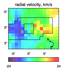
(a)	(b)

(c)

Figure 5: (a)The radial velocity field with 3 bins overplotted (3-points binning, see text); (b) fit of the ”P1” bin, representing the spectrum, ”PEGASE.HR” marking the template spectrum (shifted by -0.3 on the Flux axis from its real position, and ”Residuals” showing the difference between the fit and observed spectrum; (c) ”P1”, ”P2”, and ”P3”: co-added spectra for the 3-points binning.

Besides we will also use a tessellation of the dataset containing only three bins (3-points binning hereafter): central condensation (3 by 3 arcsec region around the centre of the galaxy), elongated disky substructure (14 by 7 arcsec) oriented according to kinematics (see section 4, Fig. 5, illustrating locations of bins and demonstrating spectra integrated in them) with the central region excluded, and the rest of the galaxy. The location of these three bins is shown in Fig. 5, and their characteristics in Table 2. Such a physically-stipulated tessellation allows to gain high signal-to-noise ratios in the bins in order to have high quality estimations of the stellar population parameters in the regions where they are expected to be homogeneous.

Bin	Nspax	m(AB)	$\mu$(AB)	S/N
P1	9	16.3	18.7	69
P2	77	15.2	19.9	49
P3	122	15.7	20.9	21

Table 2: Parameters of the ”3-points” binning: number of spatial elements, mean AB magnitude, mean AB surface brightness (mag arcsec^-2), and mean signal-to-noise ratio at 5000Å.

3 SSP age and metallicity derived from Lick indices

A classical and effective method of studying stellar population properties exploits diagrams for different pairs of Lick indices (Worthey et al., 1994). A grid of values, corresponding to different ages and metallicities of single stellar population models (instantaneous burst, SSP), is plotted together with the values computed from the observations. A proper choice of the pairs of indices, sensitive to mostly age or metallicity like H$\beta$ and Mg$b$, allows to determine SSP-equivalent age and metallicity.

We use a grid of models computed with the evolutionary synthesis code: PEGASE.HR (Le Borgne et al., 2004). These models are based on the empirical stellar library ELODIE.3 (Prugniel & Soubiran 2001, 2004) and are therefore bound to the [Mg/Fe] abundance pattern of the solar neighborhood (see Wheeler et al., 1989). To show that this limitation is not critical for our (low-mass) galaxy, Fig. 1a presents the Mg$b$ versus $<$Fe$>$ diagram with the models by Thomas et al. (2003) for different [Mg/Fe] ratios overplotted. These data allow to conclude that IC 3653 has solar [Mg/Fe] abundance ratio with a precision of about 0.05 dex.

(a)	(b)
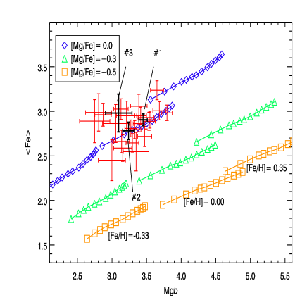
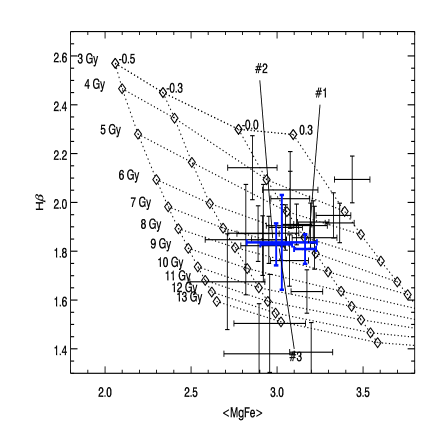
(c)	(d)

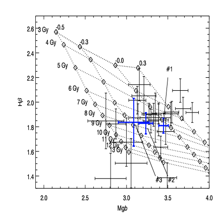
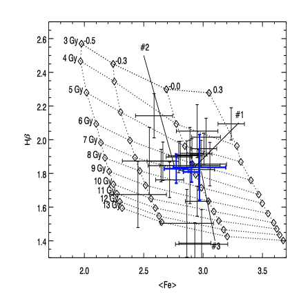
Figure 1: The Mg$b$ - $<$Fe$>^{\prime}$ (a), H${\beta}$ - [MgFe] (b), H${\beta}$ - Mg$b$ (c), and H${\beta}$ - $<$Fe$>^{\prime}$ (d) diagrams. On (a) the models from Thomas et al. (2003) are plotted. On (b), (c), and (d) the displayed grid is constructed of the values of the Lick indices for PEGASE.HR synthetic spectra (SSP) for different ages and metallicities. Bold crosses with pointers represent measurements for 3 regions of the galaxy (see text), thin crosses are for individual bins for Voronoi tessellation with target S/N=30.

A critical limitation of Lick indices is their sensitivity to missed/wrong values in the data, for example due to imperfections of the detector, or uncleared cosmic ray hits. A simple interpolation of the missed values is a poor solution, because if some important detail in the spectrum, e.g. absorption line, is affected, the final measurement of the index will be biased. In addition, the definition of the indices (see equations 1, 2, and 3 in Worthey et al. 1994) does not allow to flag or to decrease the weight of low quality values.

Due to a defect of the detector, our data have a 3pixel wide bad region (hot pixels) in the middle of the blue continuum of Mg$b$. So, strictly speaking, we could not measure Mg$b$ at all, neither H${\beta}$ on a significant part of the field of view.

As a workaround, we replaced all the missing or flagged values in the data cube by the corresponding values of the best-fitting model determined as explained in the next section. Therefore, instead of of a mathematical interpolation of missing values, we are using model predictions.

Name	bin 1	bin 2	bin 3
Ca4227	1.062 $\pm$ 0.080	0.874 $\pm$ 0.190	0.689 $\pm$ 0.700
	1.096	1.020	1.092
G4300	5.106 $\pm$ 0.135	5.042 $\pm$ 0.313	6.923 $\pm$ 1.040
	4.995	4.820	4.979
Fe4383	5.794 $\pm$ 0.176	4.940 $\pm$ 0.389	6.251 $\pm$ 1.243
	4.861	4.458	4.696
Ca4455	1.187 $\pm$ 0.089	1.096 $\pm$ 0.186	0.750 $\pm$ 0.561
	1.336	1.235	1.313
Fe4531	2.858 $\pm$ 0.125	2.326 $\pm$ 0.260	1.595 $\pm$ 0.777
	3.499	3.367	3.457
Fe4668	6.070 $\pm$ 0.181	5.776 $\pm$ 0.361	5.685 $\pm$ 1.025
	5.114	4.602	4.808
H$\beta$	1.841 $\pm$ 0.067	1.823 $\pm$ 0.122	1.800 $\pm$ 0.304
	1.908	1.966	1.878
Fe5015	5.121 $\pm$ 0.138	4.767 $\pm$ 0.246	4.912 $\pm$ 0.584
	5.491	5.211	5.292
Mg$b$	3.575 $\pm$ 0.065	3.550 $\pm$ 0.116	3.771 $\pm$ 0.278
	3.361	3.203	3.334
Fe5270	3.016 $\pm$ 0.072	2.969 $\pm$ 0.132	3.362 $\pm$ 0.309
	3.059	2.886	2.963
Fe5335	2.708 $\pm$ 0.084	2.551 $\pm$ 0.155	2.526 $\pm$ 0.367
	2.675	2.524	2.598
Fe5406	1.687 $\pm$ 0.065	1.667 $\pm$ 0.121	1.542 $\pm$ 0.286
	1.840	1.720	1.779
$<$Fe$>^{\prime}$	2.930 $\pm$ 0.075	2.852 $\pm$ 0.138	3.128 $\pm$ 0.325
	2.952	2.785	2.861
$[$MgFe$]$	3.236 $\pm$ 0.070	3.182 $\pm$ 0.127	3.435 $\pm$ 0.301
	3.150	2.987	3.089

Table 3: Measurements of selected Lick indices for the 3-points binning. All values are in Å. The first line for each index corresponds to the measurements made on the real spectra and the second on the best-fitting optimal templates (see text). (Note that the Fe indices Fe4531 and Fe5015 are essentially sensitive to titanium, see Sil’chenko & Shapovalova, 1989.)

(a)	(b)	(c)	(d)

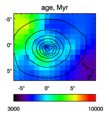
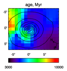
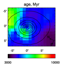
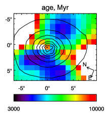
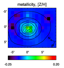
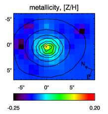
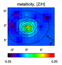
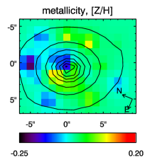
Figure 2: Maps for age and metallicity obtained by inverting bi-index grids for indices measured on optimal template spectra: (a) Mg$b$ - H${\beta}$, (b) [MgFe] - H${\beta}$, (c) $<$Fe$>$ - H${\beta}$; and on real data: (d) $<$Fe$>$ - H${\beta}$.

We measured Lick indices as defined in Trager et al. (1998), and we also derived the combined iron index $<$Fe$>^{\prime}=0.72$Fe${}_{5270}+0.28$Fe₅₃₃₅, and ”abundance-insensitive” [MgFe]$=\sqrt{\mbox{Mg}<\mbox{Fe}>^{\prime}}$ (Thomas et al. 2003). A good intermediate resolution age tracer, H${\gamma}$+Mg+Fe₁₂₅ (Vazdekis & Arimoto 1999) cannot be used, because the required signal-to-noise ratio of about 100 at around $\lambda=4340$Å cannot be achieved even after co-adding all the spectra in the data cube due to lower S/N in the blue end of the spectral range. The statistical errors on the measurements of Lick indices were computed according to Cardiel et al. (1998). Table 3 presents the measurements of selected Lick indices for the 3-points binning and Fig. 1c presents the main index-index pairs that are used to determine age and metallicity.

We see almost no population difference among three bins within the precision we reach. The age (see Table 4) is around 6 Gyr, metallicity is about solar for ”P1”, and slightly subsolar for ”P2” and ”P3”.

The large scatter of the measurements, seen on Fig. 1, results in a spread of age estimations from 4 to 13 Gyr. It is mainly caused by an imperfect cleaning of the spikes and dark pixels but also weak nebular emission may alter these indices: H$\beta$ index might be affected by emission in H$\beta$, Mg$b$ – by [NI] ($\lambda=5199$Å) laying in the red continuum region. Though we do not see any significant emission line residuals when we subtract the best fitting model, we can not exclude completely this effect.

To reduce the scatter, we measured Lick indices on the optimal templates fitted to the data. This approach may produce biased results in case of model mismatch, due for example to inconsistent abundance ratios between the models and the real stellar population. However, we believe it is not the case, since IC 3653 exhibits solar Mg/Fe abundance ratio (see Fig. 1a).

We made inversions of the bi-index grids for three combinations of indices: Mg$b$ - H${\beta}$, [MgFe] - H${\beta}$, $<$Fe$>^{\prime}$ - H${\beta}$. The maps shown in Fig. 2 represent interpolated values of the parameters between intensity-weighted centres of the bins.

The metallicity distribution shows slight gradient from -0.15 dex at the periphery to +0.10 in the very centre (the average error-bar on the metallicity measurements using [MgFe] - H${\beta}$ is 0.15 dex).

The median value for age using [MgFe] - H${\beta}$ pair is $6\pm 2.5$ Gyr, without significant spatial variation. [MgFe] and $<$Fe$>^{\prime}$ indices are not very age sensitive, thus the age estimations depend mostly on values of H${\beta}$, and are almost equal for all three pairs of indices.

4 Stellar populations and internal kinematics using pixel fitting

Various methods have been developed to determine the star formation and metal enrichment history (SFH) directly from observed spectra (Ocvirk et al. 2003, Moultaka et al. 2004, de Bruyne et al. 2004). The procedure that we are proposing here, population pixel fitting, is derived from the penalized pixel fitting method developed by Cappellari & Emsellem (2004) to determine the line-of-sight velocity distribution (LOSVD).

The observed spectrum is fitted in pixel space against the population model convolved with a parametric LOSVD. The population model consists of one or several star bursts, each of them parametrized by some of their characteristics, typically age and metallicity for a single burst while the other characteristics, like IMF, remain fixed. A single minimization returns the parameters of LOSVD and those of the stellar population.

Ideally, we would like to reconstruct SFH, over all the life of the galaxy. This means, disentangle internal kinematics and distribution in the HR diagram from the integrated-light spectrum. This problem has been discussed in several places (e. g. Prugniel et al. 2002, de Bruyne et al. 2004, Ocvirk et al. 2006), it is clearly extremely degenerated and solutions can be found only if a simplified model is fitted.

In this paper we discuss only the simplest case of SSP characterised by two parameters: age and metallicity. We do not discuss complex SFH, because signal-to-noise ratio of our data is not sufficient.

The $\chi^{2}$ value (without penalization) is computed as follows:

$$\chi^{2}=\sum_{N_{\lambda}}\frac{(F_{i}-P_{1p}(T_{i}(t,Z)\otimes\mathcal{L}(v,\sigma,h_{3},h_{4})+P_{2q}))^{2}}{\Delta F_{i}^{2}},$$ (1)

where $\mathcal{L}$ is LOSVD; $F_{i}$ and $\Delta F_{i}$ are observed flux and its uncertainty; $T_{i}$ is the flux from a SSP spectrum, convolved by the line-spread function of the spectrograph (LSF, see next subsection); $P_{1p}$ and $P_{2q}$ are multiplicative and additive Legendre polynomial of orders $p$ and $q$ for correcting a continuum; $t$ is age, $Z$ is metallicity, $v$, $\sigma$, $h_{3}$. and $h_{4}$ are radial velocity, velocity dispersion and Gauss-Hermite coefficients respectively (Van der Marel & Franx, 1993). Normally we used no additive polynomial continuum, and 5-th order multiplicative one, and for IC 3653, which has a low velocity dispersion resulting in insufficient sampling of the LOSVD, we did not fit $h_{3}$ and $h_{4}$. The problem can be partially linearized: in particular, fitting of additive polynomial continuum, and relative contributions of sub-populations $T_{i}$ is done linearly on each evaluation of the non-linear functional. Thus we end up with 10 free parameters: $t$, $Z$, 6 coefficients for $P_{mult5}$, $v$, and $\sigma$.

The main technical part of our method is a non-linear minimization procedure for $\chi^{2}$ difference between the observed and modeled spectra. The latter is made by interpolating a grid of SSP spectra computed with PEGASE.HR and degraded to match the LSF of the observed spectrum. This grid has 25 steps in age (10 Myr to 20 Gyr) and 10 steps in metallicity ([Fe/H] from -2.5 to 1.0). Because the minimization procedure requires that the derivatives of the functions are continuous, we used a two-dimensional spline interpolation. The non-linear minimization is made with the MPFIT package (by Craig B. Markwardt, NASA ) implementing constrained variant of Levenberg-Marquardt minimization.

4.1 Line spread function of the spectrograph

Before comparing a synthetic spectrum to an observation, it is required to transform it as if it was observed with the same spectrograph and setup, i. e. to degrade its resolution to the actual resolution of the observations. Actually the spectral resolution changes both with the position in the field of view and with the wavelength (thus it is not a mere operation of convolving with the LSF). Taking into account these effects is particularly critical when, as it is the case here, the physical velocity dispersion is of the same order or smaller than the instrumental velocity dispersion.

The procedure for properly taking into account the LSF goes in two steps. First, determine the LSF as a function of the position in the field and of the wavelength. Second, inject this LSF in the grid of SSP.

Therefore we made an exhaustive analysis of the LSF of our observations. A previous study of the change of the resolution of the MPFS over the field of view (Moiseev 2001) qualitatively agrees with our results.

To measure the LSF change over the field of view we used the spectra of standard stars (HD 135722 and HD 175743) and twilight sky that we analysed with our fitting procedure. The high-resolution spectra ($\Delta\lambda=0.55$Å; $R\approx 10000$) for the corresponding stars (the Sun for the twilight spectra) taken from the ELODIE.3 library (Prugniel & Soubiran 2001, 2004), were used as templates. Since these spectra have exactly the same resolution as the PEGASE.HR SSPs, the ’relative’ LSF that we determined in this way can be directly injected to the grid of SSP to make it consistent with the MPFS observations. We parametrize the LSF using $v,\sigma,h3$ and $h4$.

The whole wavelength range (4100Å– 5650Å) was splitted into five parts, overlapping by 10 per cent, and the LSF parameters were extracted in each part independently in order to derive the wavelength dependence of the LSF.

Finally, to inject the LSF in the grid of SSPs, we applied the following steps to every fiber: (i) Five convolved SSP grids were created using the LSF measured for the five wavelength ranges. (ii) The final grid was generated by linear interpolation at each wavelength point between the five grids of SSPs. For each fiber of the spectrograph this produces one grid of models matched to the LSF of the observations.

4.2 Results: kinematics, age and metallicity maps

We applied Voronoi adaptive binning procedure to our data, setting the target signal-to-noise ratio to 15. The resulting tessellation includes 76 bins with sizes from 1 to 12 pupils. To get a better presentation one may interpolate the computed values of each parameter over the whole field of view using the intensity-weighted centroids of the bins as the nodes.

We measured the systemic radial velocity $588\pm 5$km s^-1. The uncertainty includes possible systematic effects not exceeding 4 km s^-1.

The maps of radial velocity and velocity dispersions are presented in Fig. 3(d,e,f). The galaxy shows significant rotation and highly inclined disc-like structure. The uncertainties of the velocity measurements were estimated using Monte Carlo simulations and confirmed by $\chi^{2}$ maps obtained fitting only multiplicative polynomial continuum on a grid of values of age, metallicity and velocity dispersion (see appendix for details). They depend on the signal-to-noise ratio and change from 2.5 km s^-1 for the $S/N=30$ to 8 km s^-1 for the $S/N=10$.

The velocity dispersion distribution shows a gradient from 45-50 km s^-1 near the maxima of rotation to 75 km s^-1 in the core. Note a sharp peak of the velocity dispersion of 88 km s^-1 slightly shifted to the south-west of the photometric core. The uncertainties of the velocity dispersion measurements are 3.8 km s^-1 for the $S/N=30$, 5.5 km s^-1 for the $S/N=20$, and 11 km s^-1 for the $S/N=10$.

The rotation velocity and velocity dispersion profiles are shown in Fig. 4 (top pair). The rotation curve is raising to 20 km s^-1 at the edge of the field (i. e. at a radius of 5 arcsec).

The previous study of IC 3653 was made using long-slit spectroscopy (Simien & Prugniel, 2002) under poor atmosphere conditions (6 arcsec seeing). After the proper degrade of the spatial resolution of the MPFS data the agreement with these earlier observations, both for radial velocity and velocity dispersion profiles, is excellent (Fig. 4, bottom pair).

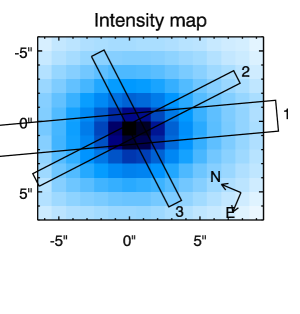
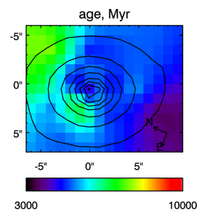
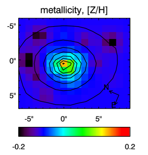
(a)	(b)	(c)
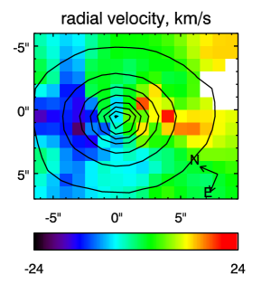
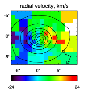
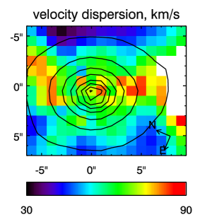
(d)	(e)	(f)

Figure 3: The generalized view of the kinematical and stellar population data. (a) intensity map with the positions the kinematical profiles are presented for: (1) position of slit in Simien & Prugniel (2002), (2) and (3) positions of major and minor axis of the embedded stellar disc; (b) map of the luminosity-weighted age distribution (in Myr); (c) map of the luminosity-weighted metallicity distribution ($[Z/\mbox{H}]$, dex); (d) radial velocity field, interpolated between the nodes of the Voronoi tessellation; (e) radial velocity field: values exactly correspond to the Voronoi tessellae; (f) velocity dispersion field, interpolated.

Figure 4: Top pair of plots: The radial velocity profile for the slice ”2” (major axis of the embedded disc) and velocity dispersion profiles for the slices ”2” and ”3” (major and minor axes of the embedded disc). Bottom pair of plots: comparison of the kinematical profiles (slice ”1”, major axis of main galactic body) to Simien & Prugniel (2002): radial velocity and velocity dispersion.

5 Photometry and morphology from ACS images

We have used ACS images from the HST archive, proposal 9401, ”The ACS Virgo Cluster Survey” by Patrick Côté. The photometric analysis of IC 3653 is not included in Côté et al. 2004. We have converted ACS counts into corresponding ST magnitudes according to the ACS Data Handbook, available on-line on the web-site of STScI, and calibrated into AB magnitudes. The derived colours agree perfectly with those given in Ferrarese et al. (2006).

The F475W–F850LP colour map (equivalent to SDSS $g$-$z$, Fig. 7) reveals an elongated region with a major axis of about 7 arcsec, axis ratio $\sim 3.5$, and orientation coinciding with the kinematical disc-like feature, which is redder than the rest of the map. This colour map was obtained using Voronoi 2D binning technique applied to the F850LP image in order to reach the signal-to-noise ratio of 80 per bin.

In the age and metallicity maps derived from the MPFS data, this elongated feature is seen as a metallicity gradient because of the lower spatial resolution due to the adaptive binning. The F475W–F850LP colour difference between the nucleus and the surrounding region 5 arcsec away from the center is about 0.05 mag. Using pegase.2 templates (Fioc & Rocca-Volmerange, 1997 ) and ACS filters transmission curves (Sirianni et al. 2005) we find that this colour difference corresponds to a metallicity difference of about 0.1 dex (assuming an age of 5 Gyr as found from our spectroscopic analysis), a value consistent with the spectroscopic analysis.

We have fitted two-dimensional Sérsic profile using the GALFIT package (Peng et al. 2002). We can see significant positive residuals, representing the nucleus in the very centre (around 1.5 arcsec in size, central surface brightness ST${}_{475}\sim 16.25$ mag arcsec², slightly asymmetric and offcentered with respect to the centre of the Sérsic profile having n=1.88, $R_{e}$=6.9 arcsec, and $\epsilon$=0.11 (Sérsic index, effective radius, and ellipticity respectively; our values coincide with ones from Ferrarese et al. 2006). There are faint large-scale residuals as well, that can be explained by superposition of several components (at least two).

Then we have modeled the images by elliptical isophotes with free center and orientation. We see some isophote twist and ellipticity change in the inner region of the galaxy that may be due to the embedded disc. Main parameters of the model fitted are presented in Fig. 6. The subtraction of the model from the original image does not reveal any internal feature.

On the lower right plot in Fig. 6 the F475W light profile is shown with crosses. The solid line represents the best-fitting Sérsic profile for the whole galaxy excluding only very centre (inner 1 arcsec) with n=1.9, and dashed line gives the best-fitting (n=1.2) for the periphery of the galaxy outside 7 arcsec, i. e. beyond the disc found in the colour map. We consider this latter fit as the most representative.

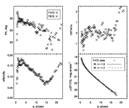
Figure 6: Photometrical characteristics of IC 3653: position angle (upper left), ellipticity of the isophotes (lower left), disky/boxy parameter a4 (upper right) in two colours, and photometric profile in F475W.

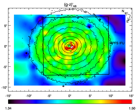
Figure 7: F475W-F850LP colour map (HST ACS data). Isophotes of the F850LP image are overimposed. The position and size of the MPFS field of view are shown.

6 Discussion

Both line-of-sight velocity field extracted from the MPFS data cube and colour map obtained from the HST imagery provide coinciding arguments for a presence of a faint internal co-rotating stellar disc embedded within a rotating spheroid. This is the main observational result from our study of IC 3653, which may be regarded to some extend as an edge-on counterpart of IC 3328, the dE with embedded spiral structure found by Jerjen et al. (2000). The disc of IC 3328 is detected to a larger radius than the one of IC 3653: the spiral structure is seen up to $\approx$ 30 arcsec = 2 $r_{e}$, while the disc of IC 3653 is detected only to 3 arcsec = 0.5 $r_{e}$. The contrast of the spiral in IC 3328 is a few per cent and in IC 3653 the disc is seen from the colour and only as a weak maximum of ellipticity at the radius of its maximum contrast to the bulge. In both galaxies, the discs are essentially stellar (no sign of star formation) and old. Estimating and comparing the mass of the two discs is strongly model-dependent, and beyond the scope of this study.

In this section we will first compare the results of two methods for estimating stellar population parameters: Lick indices and pixel-fitting, then the characteristics of IC 3653 to other dE galaxies. Finally, we will review the different possible origins of the particular properties of this galaxy.

6.1 Comparison of two techniques for estimating stellar population characteristics

In Table 4 we present comparison between SSP-equivalent age and metallicity obtained with the pixel fitting and inversion of bi-index grids for H$\beta$-Mg$b$, H$\beta$-$<$Fe$>^{\prime}$, H$\beta$-[MgFe] using index measurements on observed spectra and best-fitting templates.

One can notice particularly good agreement between the approaches. The ages derived from Lick indices appear to be slightly older, but the difference is not significant. The best agreement for both ages and metallicities is reached between pixel fitting and measurements of H$\beta$ and the combined [MgFe] index (Thomas et al. 2003). The internal precision of the parameters derived from pixel fitting is better those from Lick indices by a factor three to four, depending on the indices used. This can be explained by the optimized usage of the information by the pixel fitting procedure. Though it is difficult to assess the reliability of these small error bars, the relative variations of age and metallicity can be trusted, even when the signal-to-noise ratio is as low as 10 per pixel (with MPFS spectral resolution and wavelength coverage).

	”P1”	”P2”	”P3”
tfit, Gyr	4.93$\pm$ 0.20	4.95$\pm$ 0.30	4.97$\pm$ 0.70
tHβ-Mgb	7.04$\pm$ 1.56	6.97$\pm$ 1.47	11.25$\pm$ 6.02
t${}_{H\beta-<Fe>^{\prime}}$	7.02$\pm$ 1.33	7.28$\pm$ 2.20	6.08$\pm$ 3.94
t${}_{H\beta-\mbox{[MgFe]}}$	7.11$\pm$ 1.65	6.88$\pm$ 1.89	6.70$\pm$ 5.11
t${}_{H\beta-Mgb\mbox{mod}}$	5.27$\pm$ 1.56	5.13$\pm$ 1.47	4.85$\pm$ 6.02
t${}_{H\beta-<Fe>^{\prime}\mbox{mod}}$	5.15$\pm$ 1.33	4.30$\pm$ 2.20	4.23$\pm$ 3.94
t${}_{H\beta-\mbox{[MgFe]mod}}$	5.22$\pm$ 1.65	4.12$\pm$ 1.89	4.15$\pm$ 5.11
Zfit, dex	0.03$\pm$ 0.01	-0.14$\pm$ 0.02	-0.17$\pm$ 0.05
ZHβ-Mgb	-0.05$\pm$ 0.09	-0.18$\pm$ 0.08	-0.34$\pm$ 0.24
Z${}_{H\beta-<Fe>^{\prime}}$	-0.02$\pm$ 0.04	-0.10$\pm$ 0.05	0.03$\pm$ 0.13
Z${}_{H\beta-\mbox{[MgFe]}}$	-0.04$\pm$ 0.05	-0.14$\pm$ 0.06	-0.11$\pm$ 0.15
Z${}_{H\beta-Mgb\mbox{mod}}$	-0.02$\pm$ 0.09	-0.14$\pm$ 0.08	-0.16$\pm$ 0.24
Z${}_{H\beta-<Fe>^{\prime}\mbox{mod}}$	0.02$\pm$ 0.04	-0.14$\pm$ 0.05	-0.17$\pm$ 0.13
Z${}_{H\beta-\mbox{[MgFe]mod}}$	0.00$\pm$ 0.05	-0.13$\pm$ 0.06	-0.16$\pm$ 0.15

Table 4: Comparison of age and metallicity measurements for the 3-points binning obtained with pixel fitting and based on different pairs of Lick indices grids: measured on real spectra and on best-fitting templates.

6.2 Properties and nature of IC 3653

We computed the position of IC 3653 on the fundamental plane (FP, Djorgovski & Davis 1987). ”Vertical” deviation from FP ($d=-8.666+0.314\mu_{e}+1.14\log\sigma_{0}-\log R_{e}$, Guzman et al. 1993) is $d=0.2$. This deviation places IC 3653 into the centre of the cloud, representing dE galaxies in De Rijcke et al. (2005, their figure 2, left panel), and exactly on the theoretical predictions by Chiosi & Carraro (2002) and Yoshii & Arimoto (1987), overplotted on the same figure.

The mean age of the stellar population of IC 3653, $t=5$ Gyr, coincides with the mean age of dE galaxies in Virgo: $t_{mean}=5$ Gyr in Geha et al. (2003); $t_{mean}=5...7$ Gyr in Van Zee et al. (2004b). By contrast, the metallicity of the main body, $Z=-0.1$ is slightly higher than in these other galaxies: $Z_{mean}=-0.3$ in Geha et al. (2003); $Z_{mean}=-0.4$, Van Zee et al. (2004b). It may be understood as a consequence of the luminosity-metallicity relation if we remember that IC 3653 is more luminous than most of the galaxies in the samples of Geha et al. (2003), and Van Zee et al. (2004b).

We see that fundamental properties of IC 3653 do not differ from typical dE galaxies, though the effective radius is one of the smallest within the samples of Virgo dE’s presented in Simien & Prugniel (2002), Geha et al. (2003), and van Zee (2004a).

We derived the B-band mass-to-light ratio of IC 3653 following the method by Richstone & Tremaine (1986) as $M/L_{B}=8.0\pm 1.5(M/L_{B})_{\odot}$. The stellar mass-to-light ratio of the best fitting PEGASE.HR model in the ”P1” region is $(M/L_{B})_{*}=3.7\pm 0.4(M/L_{B})_{\odot}$. If we trust this simple dynamical model, it indicates that the dark matter content of IC 3653 is similar to recently found in De Rijcke et al. (2006) for the M 31 dE companions, i. e. about 50 per cent.

Recent theoretical studies based on N-body modelling of the evolution of disc galaxies within a $\Lambda$ CDM cluster by Mastropietro et al. (2005) suggest that discs are never completely destroyed in cluster environment, even when the morphological transformation is quite significant. Our discovery of the faint stellar disc in IC 3653 comforts these results. Thus, one of the possible origins of IC 3653 is morphological transformation in the dense cluster environment from late-type disc galaxy (dIrr progenitor). Gas was removed by means of ram pressure stripping and star formation was stopped. This process must have finished at least 5 Gyr ago, otherwise we would have seen a younger population in the galaxy. However, duration of the star formation period must have been longer than 1 Gyr, otherwise deficiency or iron (i.e. Mg/Fe overabundance) would have been observed. Within this scenario, metallicity excess in the disc can be explained by a slightly longer duration of the star formation episode compared to the spheroid. But we cannot see the difference in the star formation histories (even luminosity weighted age), because of insufficient resolution on the stellar population ages.

Another way to acquire a disc having higher metallicity than the rest of the galaxy is to experience a minor dissipative merger event (De Rijcke et al. 2004). This is rather improbable for a dwarf galaxy, but cannot be completely excluded. In particular, kinematically decoupled cores, recently discovered in dwarf and low-luminosity galaxies (De Rijcke et al. 2004, Geha et al. 2005, Prugniel et al. 2005, Thomas et al. 2006) can be explained by minor merger events.

The most popular scenario which is usually considered to explain formation of embedded stellar discs in giant early-type galaxies is star formation in situ after infall of cold gas onto existing rotating spheroid, e.g. from a gas-rich companion (cross-fueling). This scenario has been used by Geha et al. (2005) to explain counter-rotating core in NGC 770, a dwarf S0 which is more luminous than IC 3653 ($M_{B}=-18.2$ mag) and located close to a massive spiral companion NGC 772 ($M_{B}=-21.6$ mag) in a group. In NGC 127 ($M_{B}=-18.0$ mag), a close satellite of another giant gas-rich galaxy, NGC 128, we observe the process of cross-fueling at present (Chilingarian, 2006). Group environment, where relative velocities of galaxies are rather low, favours of the interaction processes on large timescales, such as smooth gas accretion.

Our data on IC 3653 cannot provide a decisive choice between those alternatives. However, from a general point of view, dynamically hot environment of the Virgo does not favour the slow accretion of cold gas. IC 3653 is not a member of a subgroup including large galaxies, which can foster gaseous disc, so we believe that in this particular case the scenario of slow accretion is not applicable.

At present, the sample of objects where disc-like sub-structures were searched either from images or integral field spectroscopy is still too small to draw statistical conclusions. But it is quite probable that the progenitors of the dE’s were disc galaxies (pre-dIrr or small spiral galaxies) and that they evolved due to feedback of the star formation and environmental effects. Present dIrr also experienced feedback but kept their gas, so it is unlikely that the feedback alone can remove the gas. Therefore environmental effects are probably the driver of the evolution of dE’s, and the discovery of stellar discs in dE’s is consistent with this hypothesis.

Appendix A Validation and error analysis

In this appendix we address questions concerning the error analysis, stability of the solutions, and possible biases for relatively old stellar population (about 5 Gyr). A full description of these aspects extended to any instrument and much wider range of parameters will be described in details in the forthcoming paper (Koleva et al. in preparation). Here we give only essential error analysis required for validation of the results presented in this paper and in the forthcoming papers based on MPFS data for dwarf galaxies.

A.1 Error analysis

Error estimates on the stellar population parameters is complicated because of the internal degeneracies and coupling, and the questions of unicity of the solution and local minima are always critical. A complete and detailed description of one of the possible approaches to locate the alternate solutions using for a allied inversion technique is given in Moultaka & Pelat (2000).

We performed some Monte-Carlo simulations (about 10000 per spectrum for the 3-points binning) to demonstrate the consistency between the uncertainties on the parameters reported by the minimization procedure and the real error distributions. These simulations have demonstrated that in case of our dataset, where there is neither significant model mismatch due to element abundance ratios, nor strong mistake with subtraction of additive terms (diffuse light and night sky), the uncertainties found from the Monte-Carlo simulations using scattering of solutions in the multidimensional parameter space coincide with values reported by the minimization procedure being multiplied by $\chi^{2}$ values. Deviation of $\chi^{2}$ from 1 might be caused either by poor quality of the fit (model-mismatch) or by wrong estimations of absolute flux uncertainties in the input data. We inspected the residuals of the fit visually and by averaging them using wide smoothing window (150 pixels) and found no significant deviations between model and observations. Thus we conclude that in some cases our estimations of the uncertainty on the absolute fluxes based on the photon statistics may be wrong by 15 per cent, resulting in values of $\chi^{2}$ between 0.7 and 1.3.

To estimate the errors more accurately, locate possible alternate solutions and search for degeneracies between kinematical and stellar population parameters we study the distribution of $\chi^{2}$ in the age – metallicity – velocity dispersion space. The procedure we followed includes the following steps:

• We chose a grid of values for age, metallicity, and velocity dispersion, that was supposed to cover a reasonable region of the parameter space where we could expect to have solutions. In our case the grid was defined as: 2 Gyr $<$ t $<$ 14 Gyr with a step of 200 Myr, -0.45$<$[Fe/H]$<$0.40 with a step of 0.01 dex, 30 km s^-1 $<$ $\sigma$ $<$ 100 km s^-1 with a step of 0.5 km s^-1

• At every node of t-Z grid we ran the pixel fitting procedure in order to determine multiplicative polynomial continuum, and to have the best fit for a given SSP

• Later $\chi^{2}$ was computed on the grid of values of $\sigma$ by fixing all other components of the solution that had been found in the previous step

The reason to scan the $\sigma$ dimension with fixed multiplicative polynomial is to save computer time by reducing the number of free parameters, and it is justified by the strong decoupling between the multiplicative polynomial (affecting only low frequencies) and the velocity dispersion (affecting high frequencies).

In other words using our procedure we compute a slice of the full $\chi^{2}$ by the hypersurface defined as a set of minimal $\chi^{2}$ values for multiplicative continuum terms and radial velocity values, and then reproject it onto ”t-Z” and ”t-Z-$\sigma$” hyperplanes. The result contains two arrays: 2D age-metallicity and 3D age-metallicity-velocity dispersion.

The values of line-of-sight radial velocity obtained during the fitting procedure on the ”t-Z” grid are constant within the errors, suggesting that scanning of the $\chi^{2}$ hyperspace on $v$ is not necessary.

In Fig. 8 (upper line) we present the maps of $\chi^{2}$ for the 3-points binning on the ”t-Z” plane. One can see elongated shapes of the minima, corresponding to well known age-metallicity degeneracy. Three plots on the bottom of Fig. 8 represent slices of the 3D $\chi^{2}$ space scan (t-Z-$\sigma$) for the ”P1” bin. One can notice that the width of the minimum on ”t-Z” plane has decreased due to a correlation between metallicity and velocity dispersion, that is clearly seen on the ”Z-$\sigma$” slice. This degeneracy between velocity dispersion and metallicity can be understood as follows: an overestimate of the metallicity in the template increases depth of the absorption lines and can be compensated by higher velocity dispersion. In principle an important mismatch of the metallicity when analysing the kinematics with usual methods may bias the velocity dispersion and even produce patterns in velocity dispersion profiles, whereas it is in reality a metallicity gradient. A mismatch of 0.1 dex results in a bias of 15 per cent on the velocity dispersion.

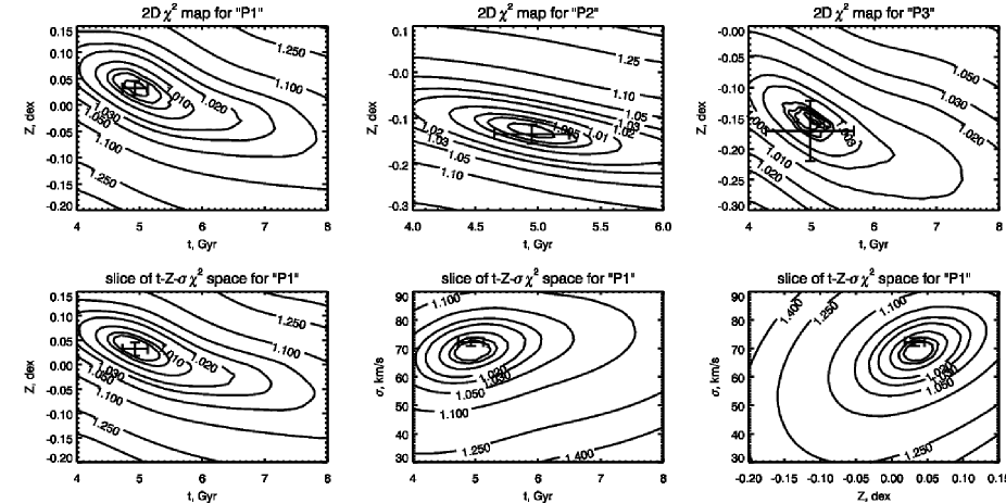
Figure 8: 2-dimensional maps of $\chi^{2}$ distributions for the 3-points binning (upper row), and slices of the 3-dimensional $\chi^{2}$ distribution (t-Z-$\sigma$) for the ”P1” bin.

A.2 Stability of solutions

Stability of solutions is a crucial point for every method dealing with multiparametric non-linear minimization. We studied the stability with respect to initial guess, wavelength range being used, and degree of the multiplicative polynomial continuum.

A.2.1 Initial guess

We have made several dozens of experiments with different initial guesses in order to inspect the stability of convergence. We found a correct convergence for a wide range of guesses of age, metallicity and velocity dispersions, but for radial velocity the initial guess must be within twice the velocity dispersion from the solution.

A.2.2 Wavelength range

We ran two series of experiments: one with $\lambda>4700$Å, and another one with the full wavelength range, but regions of Balmer lines (H$\gamma$ and H$\beta$) masked. The first experiment checks the sensitivity to the wavelength range (several strong metallic features are excluded) and the second one removes the best age estimators (Worthey at al. 1994, Vazdekis & Arimoto 1999), so that instability on age may be expected.

The first experiment does not reveal any bias, but only an expectable increase of the uncertainties.

The second experiment does not neither reveal instability, but though the errors on metallicity and velocity dispersion are not strongly affected, the error on age is multiplied by 3 (therefore the precision become comparable to Lick indices). It is remarkable that even without Balmer lines it is possible to give estimations of age of the stellar population.

	P1	P2	P3
$v$, km s-1	601.8$\pm$ 1.0	603.4$\pm$ 1.4	603.8$\pm$ 3.0
	600.9$\pm$ 1.0	603.1$\pm$ 1.7	603.7$\pm$ 3.4
$\sigma$, km s-1	70.9$\pm$ 1.6	67.3$\pm$ 2.2	52.1$\pm$ 5.0
	71.8$\pm$ 1.6	65.3$\pm$ 2.6	52.1$\pm$ 5.7
t, Gyr	4.855$\pm$ 0.218	4.728$\pm$ 0.289	4.629$\pm$ 0.694
	4.714$\pm$ 0.235	4.448$\pm$ 0.403	4.238$\pm$ 0.930
Z, dex	0.01$\pm$ 0.02	-0.14$\pm$ 0.02	-0.15$\pm$ 0.05
	0.03$\pm$ 0.01	-0.13$\pm$ 0.02	-0.15$\pm$ 0.05

Table 5: Stability of the solutions for the 3-points binning with respect to the wavelength range. First lines for every parameter correspond to $\lambda>4700$Å, second ones to full range with Balmer lines excluded.

A.2.3 Order of multiplicative polynomial continuum

We also explored the stability of the method with respect to the order of the multiplicative polynomial continuum. The results are shown in Fig. 9. One can see that for n$>$5 there is neither significant changes of the estimations of kinematical and stellar population parameters, nor of $\chi^{2}$ value. Therefore we chose $n=5$ for all our data analysis.

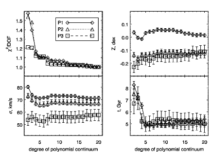
Figure 9: Stability of the parameters with respect to the order of the multiplicative polynomial continuum. Different plotting symbols correspond to three bins of the 3-points binning.

A.3 Possible biases

There are several possible sources of systematic errors on the parameters: (1) additive systematics of the flux calibration due to under- or oversubtraction of the night sky, (2) imperfections of the models, one of the most important among those is non-solar abundance ratio. Since IC 3653 exhibits exactly solar [Mg/Fe] (see Fig. 1) everywhere in the field of view, we do not study possible consequences of abundance ratio mismatch in this paper.

The accurate subtraction of the night sky emission is a challenging step of the data reduction for low-surface brightness objects. Basically, night sky emission consists of continuum emission, that might include scattered solar light as well, and several bright emission lines. Under- or oversubtraction of night sky brings additive component resulting in changing the relative depths of spectral features, and therefore affects particularly the estimates of the metallicity.

We have conducted two series of experiments: (1) adding a constant term or (2) the spectrum itself smoothed by a 300 pixels window to simulate the diffuse light in the spectrograph. In every series the fraction of the additive term was between -20 and +50 per cent to model over- and undersubtraction. The results for the constant term as a fraction of flux at 5000Å are shown in Fig. 10. One may notice that $\chi^{2}$ reaches minimum on slightly negative (over-subtraction) values of the additive term because we did not change flux uncertainties during our experiments. The remarkable result is the stability of age estimations on a wide range of additive components (-25 to 15 per cent). This is an important advantage of the pixel-fitting technique over Lick indices, more sensitive to additive continuum. Metallicity and velocity dispersion exhibit the expected behaviour: growth of $\sigma$ and fall of Z. Indeed within a range of contribution between -5 and 5 per cent changes are quite small ($\sim$8 per cent for $\sigma$, and $\sim$0.1 dex for Z) though significant.

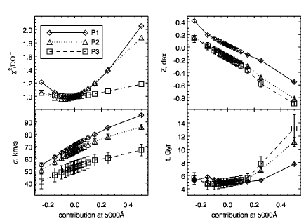
Figure 10: Effects of additive terms on the results. Abscissa represents the contribution of the constant level at $\lambda$=5000Å. Different plotting symbols correspond to each bin of the 3-points binning.

In order to test the consequences of bad sky subtraction we made two additional experiments: we tried to fit the data, where the sky spectrum was represented by a low-order polynomial continuum and with no sky subtraction at all. We excluded four regions of the spectrum containing bright emission lines: HgI $\lambda=$4358Å, 5461Å, [NI] $\lambda=$ 5199Å, and [OI] $\lambda=$ 5577Å. The experiments were made for the 3-points binning of the data, demonstrating the effects for high, intermediate, and low surface brightness (see Table 2). Basically we found no significant difference for the ”P1” and ”P2” bins between the parameters for the correct sky subtraction and subtraction of the low-order polynomial model of the sky (see Table 6). ”P3” bin gives younger age and higher metallicity, but the estimations are in agreement with the normal sky subtraction within 2$\sigma$ However, as expected, when sky is not subtracted at all we find sizeable bias on age, metallicity, and velocity dispersion estimations for the ”P2” bin, and even stronger effect for ”P3”. Due to additive continuum metallicities are found to be lower, ages older, and velocity dispersions higher than expected. These experiments demonstrate that for the surface brightness down to $\mu_{B}=20$ mag arcsec^-2 features of the night sky spectrum do not affect the results of the pixel fitting procedure, and very rough sky subtraction is sufficient to obtain the realistic estimations of kinematical and stellar population parameters.

	P1	P2	P3
$v$, km s-1	604.3$\pm$ 1.0	606.0$\pm$ 1.5	609.4$\pm$ 3.2
	604.4$\pm$ 1.0	605.9$\pm$ 1.6	610.3$\pm$ 3.7
$\sigma$, km s-1	71.5$\pm$ 1.5	64.9$\pm$ 2.4	54.4$\pm$ 5.2
	80.5$\pm$ 1.5	88.3$\pm$ 2.2	105.5$\pm$ 4.6
t, Gyr	4.868$\pm$ 0.210	4.547$\pm$ 0.310	3.956$\pm$ 0.731
	4.972$\pm$ 0.185	7.203$\pm$ 0.390	12.982$\pm$ 1.641
Z, dex	0.04$\pm$ 0.01	-0.10$\pm$ 0.02	-0.06$\pm$ 0.04
	-0.08$\pm$ 0.01	-0.50$\pm$ 0.02	-0.94$\pm$ 0.03

Table 6: Determination of the kinematical and stellar population parameters for a case of polynomial night sky model (first line for every parameter) and no sky subtraction (second line for every parameter).

References

- Barazza et al., (2002) Barazza F. D., Binggeli B., Jerjen H., 2002, A&A, 391, 823
- Bertola & Capaccioli, (1971) Bertola F., Capaccioli, M., 1975, ApJ, 200, 439
- Bertola & Galletta, (1978) Bertola F., Galletta, 1978, ApJ, 226, L115
- Binggeli et al., (1985) Binggeli B., Sandage A., Tammann G. A., 1985, AJ, 90, 1681
- Binggeli et al., (1990) Binggeli B.; Tarenghi M., Sandage A., 1990, A&A, 228, 42
- Binney, (1976) Binney, J., 1976, MNRAS, 177, 19
- Cappellati & Copin, (2003) Cappellari M., Copin Y., 2003, MNRAS, 342, 345
- Cappellari & Emsellem, (2004) Cappellari M., Emsellem E., 2004, PASP, 116, 138
- Cardiel et al., (1998) Cardiel N., Gorgas J., Cenarro J., González J.J., 1998, A&AS, 127, 597
- Chiosi & Carraro, (2002) Chiosi, C., Carraro, G. 2002, MNRAS, 335, 335
- Chilingarian, (2006) Chilingarian I., 2006, PhD Thesis, astro-ph/0611893
- Conselice et al., (2001) Conselice C., Gallagher J., Wyse R., 2001, ApJ, 559, 791
- Conselice et al., (2003) Conselice C., O’Neil K., Gallagher J., Wyse R., 2003, ApJ, 591, 167
- Côté et al. (2004) Côté P., Blakeslee J., Ferrarese L., Jordán A., Mei S., Merritt D., Milosavljević, M., Peng E., Tonry J., West M., 2004, ApJS, 153, 223
- de Bruyne et al., (2003) de Bruyne V., de Rijcke S., Dejonghe H., Zeilinger W. W., 2003, MNRAS, 349, 461
- De Rijcke et al., (2001) De Rijcke S., Dejonghe H., Zeilinger W.W., Hau G., 2001, ApJ, 559, L21
- De Rijcke et al., (2004) De Rijcke S., Dejonghe H., Zeilinger W. W., Hau G. K. T., 2004, A&A, 426, 53
- De Rijcke et al., (2006) De Rijcke S., Prugniel Ph., Simien F., Dejonghe H., 2006, MNRAS, 369, 1321
- Djorgovski & Davis, (1987) Djorgovski S., Davis M., 1987, ApJ, 313, 59
- Duc & Mirabel, (1999) Duc P.-A., Mirabel I. F., 1999, Proceedings of IAU Symposium 186, 61
- Ferrara & Tolstoy, (2000) Ferrara A., Tolstoy E., 2000, MNRAS, 313, 291
- (22) Ferrarese L., Côté P., Jordan A., Peng E., Blakeslee J., Piatek S., Mei S., Merritt D., Milosavljevic M., Tonry J., West M., 2006, in press, astro-ph/0602297
- Fioc & Rocca-Volmerange, (1997) Fioc M., Rocca-Volmerange B.; 1997, A&A, 326, 950
- Gavazzi et al., (2003) Gavazzi G., Boselli A., Donati A., Franzetti P., Scodeggio M., 2003, A&A, 400, 451
- Geha et al., (2002) Geha M., Guhathakurta P., van der Marel R.P., 2002, AJ, 124, 3073
- Geha et al., (2003) Geha M., Guhathakurta P., van der Marel R.P., 2003, AJ, 126, 1794
- Geha et al., (2005) Geha M., Guhathakurta P., van der Marel R.P., 2005, AJ, 129, 2617
- Gorgas et al., (1997) Gorgas J., Pedraz S., Guzmán R., Cardiel N., González J.J., 1997, ApJ, 481, L19
- Guzmán et al. (1993) Guzmán, R., Lucey, J. R., Bower, R. G. 1993, MNRAS, 265, 731
- Held & Mould, (1994) Held E., Mould J., 1994, AJ, 107, 1307
- Illingworth, (1977) Illingworth G., 1977, ApJ, 218, L43
- (32) Koleva M., Ocvirk P., Le Borgne D., Prugniel P., Chilingarian I., Soubiran C., in preparation
- Jerjen et al., (2000) Jerjen H., Kalnajs A., Binggeli B., 2000, A&A, 358, 845
- Le Borgne et al., (2004) Le Borgne D., Rocca-Volmerange B., Prugniel P., Lanc̣on A., Fioc M., Soubiran C., 2004, A&A, 425, 881
- Lisker et al. (2006) Lisker T., Grebel E., Binggeli B., 2006, AJ, 132, 497
- Malin & Carter, (1983) Malin D. F., Carter D., 1983, ApJ, 274, 534
- Marcolini et al., (2003) Marcolini A., Brighenti F., D’Ercole, A., 2003, MNRAS, 345, 1329
- Mastropietro et al., (2005) Mastropietro C., Moore B., Mayer L., Debattista V., Piffaretti R., Stadel J., 2005, MNRAS, 364, 607
- Michielsen et al., (2003) Michielsen D., de Rijcke S., Dejonghe H., Zeilinger W. W., 2003, ApJ, 597, L21
- Michielsen et al., (2004) Michielsen D., de Rijcke S., Zeilinger W. W., Prugniel Ph., Dejonghe H., Roberts, S., 2004, MNRAS, 311, 1293
- Moiseev, (2001) Moiseev A. V., 2001, BSAO, 51, 140
- Moore et al. (1998) Moore B., Lake G., Katz N., 1998, ApJ, 495, 139
- Moultaka & Pelat, (2000) Moultaka J., Pelat D., 2000, MNRAS, 314, 409
- Moultaka et al., (2004) Moultaka J., Boisson C., Joly M., Pelat D., 2004, A&A, 420, 459
- (45) Ocvirk P., Pichon C., Lanc̣on, A., Thiébaut E., 2003, MNRAS, 365, 46
- (46) Ocvirk P., Pichon C., Lanc̣on, A., Thiébaut E., 2003, MNRAS, 365, 74
- Paturel et al. (2003) Paturel G., Petit C., Prugniel Ph., Theureau G., Rousseau J., Brouty M., Dubois P., Cambresy L., 2003, A&A, 412, 45
- Pedraz et al., (2002) Pedraz, S., Gorgas, J., Cardiel, N., Sánchez-Blázquez, P., Guzmán, R., 2002, MNRAS, 332, L59
- Peng et al. (2002) Peng C., Ho L. C., Impey C. D., Rix H.-W., 2002, AJ, 124, 266
- Prugniel et al., (2005) Prugniel P., Chilingarian I., Sil’chenko O., Afanasiev V., 2005, Proceedings of IAU Colloquium 198, 73
- Prugniel & Soubiran, (2001) Prugniel P., Soubiran C., 2001, A&A, 369, 1048
- Prugniel & Soubiran, (2001) Prugniel P., Soubiran C., 2004, astro-ph/0409214
- Richstone & Tremaine, (1986) Richstone D., Tremaine S., 1986, AJ, 92, 72
- Sadler & Gerhard, (1985) Sadler, E. M.; Gerhard, O. E., 1985, MNRAS, 214, 177
- Sil’chenko & Shapovalova, (1989) Sil’chenko O., Shapovalova A., 1989, SoSAO, 60, 44
- Simien & Prugniel, (2002) Simien F., Prugniel, Ph., 2002, A&A, 384, 371
- Sirianni et al., (2005) Sirianni M., Jee M. J., Benétez N. et al., 2005, PASP, 117, 1049
- Thomas et al., (2003) Thomas D., Maraston C., Bender R., 2003, MNRAS, 339, 897
- Thomas et al., (2006) Thomas D., Brimioulle F., Bender R., Hopp U., Greggio L., Maraston C., Saglia R. P., 2006, A&A, 445, L19
- van den Bergh, (1994) van den Bergh S., 1994, ApJ, 428, 617
- (61) van Zee L., Skillman E. D., Haynes, M. P., 2004, AJ, 128, 121
- (62) van Zee L., Barton E. J., Skillman E. D., 2004, AJ, 128, 2797
- van der Marel & Franx, (1993) van der Marel R., Franx M., 1993, ApJ, 407, 525
- Vazdekis & Arimoto, (1999) Vazdekis A., Arimoto N., 1999, ApJ, 525, 144
- Weilbacher et al., (2000) Weilbacher P. M., Duc P.-A., Fritze von Alvensleben U., Martin P., Fricke K. J., 2000, A&A, 358, 819
- Wheeler et al. (1989) Wheeler J. C., Sneden C., Truran J. W. Jr., 1989, ARA&A, 27, 279
- Worthey, (1994) Worthey G., 1994, ApJS, 95, 107
- Worthey et al., (1994) Worthey G., Faber S., González J., Burstein D., 1994, ApJS, 94, 687
- (69) Yoshii, Y., Arimoto, N. 1987, A&A, 188, 13