Spiral shocks and the formation of molecular clouds in a two phase medium

Abstract

We extend recent numerical results (Dobbs et al., 2006) on molecular cloud formation in spiral galaxies by including a multi-phase medium. The addition of a hot phase of gas enhances the structure in the cold gas, and significantly increases the fraction of molecular hydrogen that is formed when the cold gas passes through a spiral shock. The difference in structure is reflected in the mass power spectrum of the molecular clouds, which is steeper for the multi-phase calculations. The increase in molecular gas occurs as the addition of a hot phase leads to higher densities in the cold gas. In particular, cold gas is confined in clumps between the spiral arms and retains a higher molecular fraction. Unlike the single phase results, molecular clouds are present in the inter-arm regions for the multi-phase medium. However the density of the inter-arm molecular hydrogen is generally below that which can be reliably determined from CO measurements. We therefore predict that for a multi-phase medium, there will be low density clouds containing cold atomic and molecular hydrogen, which are potentially entering the spiral arms.

1 Introduction

Numerical simulations have become a powerful tool to explore the physics of star formation (Ostriker et al., 2001; Bate et al., 2003; Mac Low & Klessen, 2004; Bonnell et al., 2007). Recent advances in computational power now make it possible to study the formation of giant molecular clouds (GMC) and the onset of star formation (Kim et al., 2003; Bonnell et al., 2006; Dobbs et al., 2006; Glover & Mac Low, 2006a, b; Vazquez-Semadeni et al., 2006). There are two general formation mechanisms that have been advanced. the first is that a cloud becomes self-gravitating, inducing high-densities and the conversion of HI into molecular gas. The second possibility is that an external triggering such as a spiral or other turbulent shock either gathers together pre-existing molecular gas (Pringle et al., 2001) or induces high densities in the shock and thus converting HI into H2.

Previous results show that spiral shocks induce the formation of dense molecular clouds (Dobbs et al., 2006) and simultaneously generate a velocity dispersion (Bonnell et al., 2006). A prerequisite for the formation of these molecular clouds in isothermal simulations is that the gas is cold, of order 100 K or less (Dobbs et al., 2006). For cold gas, the densities in the shocks are sufficiently high for H₂ formation, and the dynamics of the spiral shocks lead to clumpy structures in the gas. The cold atomic component of the ISM contains the most mass of atomic hydrogen in the ISM, but the filling factor of this phase is very small ($\sim 0.013$, Cox 2005). The warm ($10^{4}$K) atomic phase, which is typically used in simulations of spiral galaxies (Kim & Ostriker, 2002; Wada & Koda, 2004; Gittins & Clarke, 2004), contains less mass but fills just over a third of the volume of the ISM (Cox, 2005). The simulation described in this paper is the first to examine the dynamics of a spiral potential with both cold and warm phases. The resulting gas distribution is more representative of the ISM, with cold gas embedded in smaller clumps within a warm diffuse phase.

In the present study, we investigate the effects of the hot medium on a pre-existing cold HI as it passes through the spiral shock. The motivation is to include the pressure confinement of the hot gas in the dynamics of a spiral shock. We do not include any transition between the hot and cold components but rather assume the picture presented by (Pringle et al., 2001) that molecular clouds are formed from gas that is cold before it enters the shock. We leave a full treatment of the thermal evolution of the gas to a later study. Glover & Mac Low (2006a, b) analyze molecular cloud formation over much smaller size-scales (20-40 pc), but include a more consistent treatment of the ISM and H₂ formation. In their models, molecular clouds form slowly in gravitationally collapsing uniform gas (Glover & Mac Low, 2006a) or rapidly from the compression of turbulent gas (Glover & Mac Low, 2006b). The gas temperature in these calculations is initially $10^{4}$ K, but quickly drops to 100 K or less once the density exceeds 1 cm^-3. Other models of the ISM have shown the formation of cold ($<100$ K) HI, as a precursor to molecular clouds, on local (Vazquez-Semadeni et al., 1995; Audit & Hennebelle, 2005; Heitsch et al., 2005) and galactic (Wada & Norman, 1999) scales.

We present numerical results to investigate the dynamics of cold gas subject to a spiral shock when in the presence of a confining warm phase. We compare this 2 phase simulation of a galactic disc with the previous single phase simulations shown in Dobbs et al. (2006). In particular, we describe the structure of molecular clouds and the content of molecular hydrogen across the galactic disc. We also provide the first attempts to determine individual molecular cloud properties from global simulations.

2 Calculations

We use the 3D smoothed particle hydrodynamics (SPH) code based on the version by Benz (Benz, 1990). The smoothing length is allowed to vary with space and time, with the constraint that the typical number of neighbours for each particle is kept near $N_{neigh}\thicksim 50$. Artificial viscosity is included with the standard parameters $\alpha=1$ and $\beta=2$ (Monaghan & Lattanzio, 1985; Monaghan, 1992).

2.1 Flow through galactic potential

The galactic potential includes spiral components for the disc, dark matter halo and spiral density pattern. The potential is described in full in Dobbs et al. (2006). The spiral component has 4 spiral arms and is taken from Cox & Gómez (2002). The amplitude is 1 atom cm^-3, the pattern speed is $2\times 10^{-8}$ rad yr^-1 and pitch angle $\alpha=15^{o}$. The pattern speed leads to a co-rotation radius of 11kpc. The disc is in equilibrium, as the rotational velocities of the gas balance the centrifugal force of the potential.

Self-gravity magnetic fields, heating, cooling or feedback from star formation are not included in these calculations. We further neglect pressure due to cosmic rays, which contributes tot the pressure of the diffuse ISM. The paper instead focuses on how hydrodynamic forces and the galactic potential influence the flow.

2.2 Initial conditions and calculation of molecular gas density

Gas particles are initially distributed as described in Dobbs et al. (2006), occupying a region of radius 5 kpc$<r<$10 kpc. The disc has a scale height $z\leq 100$ pc, and a velocity dispersion of 2.5% of the orbital speed for the $z$ component of the velocities maintains vertical equilibrium. We determine the $x$ and $y$ components of the positions and velocities from a 2D test particle run. Particles in the test run are initially distributed uniformly with circular velocities. They evolve for a couple of orbits subject to the galactic potential, to give a spiral density pattern with particles settled into their perturbed orbits. A velocity dispersion of 2.5% of the orbital speed is also added to the $x$ and $y$ velocities.

The gas is distributed in 2 phases, a cold component of $T=100$ K, and a warm component of $T=10^{4}$ K. Each phase constitutes half of the gaseous mass of the disc, $5\times 10^{8}$ M_⊙, so the total mass of the disc is $10^{9}$ M_⊙. This corresponds to a nominal surface density of $\sim 4$ M_⊙ pc${}^{{}_{2}}$ ($9\times 10^{-4}$ g cm^-2). The total HI surface density at the solar radius is $\sim 5$ M_⊙ pc${}^{{}_{2}}$ (Wolfire et al., 2003). The SPH particles are initially randomly assigned as hot or cold gas, but the distribution settles into a diffuse warm and dense cold phase as the simulation progresses. The gas is isothermal for both phases. The calculation of the smoothing lengths does not distinguish between cold and hot particles. Using two phases can lead to numerical issues with the smoothing lengths (Thacker et al., 2000), in particular overcooling, although both phases are isothermal in our simulations. Furthermore only a small fraction of cold particles have predominantly hot neighbours e.g. only 2 % of cold particles have $<20$% cold neighbours.

Ideally, a full treatment of the ISM, which includes heating and cooling between the two phases should be applied. However, the primary aim of this paper is to investigate how a hot phase affects the dynamics of cold gas passing through a spiral shock. There have been recent theoretical arguments that molecular clouds may form from cold HI or molecular gas (Pringle et al., 2001), motivated by observational evidence for shorter cloud lifetimes. Observations also imply that molecular clouds form from molecular gas in M51 (Vogel et al., 1988), and thre may be reservoirs of low density H₂ present in galaxies which is difficult to detect (Lequeux et al., 1993; Allen et al., 2004). Cold HI is ubiquitous in the Outer Galaxy (Gibson et al., 2006) and appears to be flowing into the spiral arms (Gibson et al., 2005).

We calculate the density of molecular hydrogen by the same process as described in Dobbs et al. (2006). We post-process our results to determine the fraction of molecular gas, using the equation for the rate of change of H₂ density from Bergin et al. (2004)

$$\frac{dn(H_{2})}{dt}=R_{gr}(T)n_{p}n(H)-[\zeta_{cr}+\zeta_{diss}(N(H_{2}),A_{V})]n(H_{2}).$$ (1)

The total number density is $n_{p}$, where $n_{p}=n(H)+2n(H_{2})$, $N$ is the column density (of atomic or molecular hydrogen) and $T$ the temperature. The strength of the UV field is $\zeta_{diss}(0)=4.17\times 10^{-11}$ s^-1, comparable with the UV flux from a B0 star, and the cosmic ray ionization rate is $\zeta_{cr}=6\times 10^{-18}$ s^-1. There is some uncertainty in the cosmic ray ionization rate (e.g. Le Petit et al. 2004) but this term is much less than the the other components of Eqn. 1 and unlikely to affect our results. $R_{gr}$ is the formation rate on grains, assuming an efficiency of $S=0.3$. We do not explicitly change $S$ for the warm gas in our calculations, but the density of the warm gas is too low for H₂ formation to occur (Dobbs et al., 2006) and H₂ is dissociated at high temperatures. Ideally, a more realistic treatment of the ISM including heating and cooling should be included for a more accurate calculation of H₂ formation. However, as shown in Dobbs et al. (2006), this method primarily extracts the densest gas.

Our main simulation was performed with 6 million particles, 3 million in each of the hot and cold phases. This compares to our previous single-phase simulation of 4 million cold particles (Dobbs et al., 2006). In addition to these high resolution runs, we ran lower resolution runs (of 1 million and 250,000 particles) to investigate the effects of the numerical resolution. The lower resolution runs generally yield lower maximum densities throughout and lower H₂ fractions.

Figure 1: Column density plots (g cm^-2) showing a 5 kpc by 5 kpc section of the disc (with Cartesian coordinates -9 kpc $<x<$ -4 kpc and -5 kpc $<y<$ 0 kpc. The xy-coordinate grid is centred on the midpoint of the disc and remains fixed with time. Gas is flowing clockwise across the disc, i.e. from bottom to top. The time corresponding to each plot is i) 60 Myr, ii) 140 Myr and iii) 220 Myr. The plot shows the total column density, including both the 100 and 10⁴ K components.

3 Results

We first discuss the overall structure of the disc and the overall distribution of molecular hydrogen. In Section 3.5, we use a clump-finding algorithm to determine the properties of individual molecular clouds. We compare results from the multiphase calculation and the single phase (50 K) simulation described in Dobbs et al. (2006). In Sections 3.3 and 3.6.1 we compare the inter-arm and arm molecular gas densities for the multi-phase simulation with observational results, and comment on the ratio of inter-arm to arm molecular clouds.

3.1 Structure of the disc

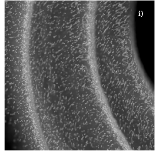
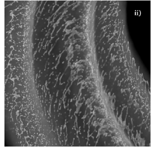
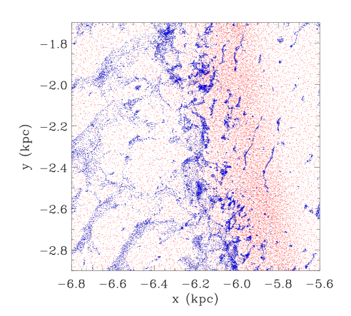
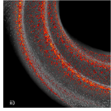
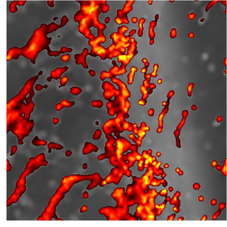
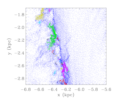
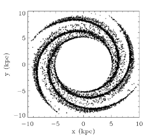
The column density section of the disc of the multi-phase simulation is shown in Fig. 1 at different times. From Fig. 1, we see the growth of small scale structures into self consistent, large scale features over time. The figure includes both the 100 and $10^{4}$ K gas. The 100 K gas is most clearly visible in small clumps whilst the $10^{4}$ K gas provides a diffuse background and the smooth component of the spiral arms. The 2 components are shown explicitly in Fig. 2, which plots the particles representing the hot and cold gas separately for a section of the disc after 100 Myr. Both figures show that the cold gas is confined by the pressure from the hot component into small dense clumps. The hot gas on the other hand is much more uniform and smooth. As previously described (Dobbs et al., 2006), the structure of the gas in the spiral arms is dependent on the gas dynamics of the spiral shock. For cold gas, the spiral shock increases clumpy structure in the gas. For hot gas the shock is much weaker, so has much less effect on the dynamics, and the gas pressure will smooth out any structure in the gas (Dobbs & Bonnell, 2006). Two further differences are apparent for the spiral shock for each component. As can be seen in Fig. 2, the shock for the cold gas is offset from the shock corresponding to the hot gas. However the shock from the hot component is evidently affecting the cold gas clumps, as can be seen from the elongation of the cold gas clumps as they enter the spiral arm (Fig. 2). The shock for the hot gas is also much wider than for the cold gas, since the degree of compression of the hot gas is much less, whilst the cold gas forms a very narrow spiral arm.

Fig. 3 shows the distribution of mass with density for the multi and single phase simulations after 100 Myr. The hot component contributes a greater mass at low densities for the multi-phase simulation. The greater mass at high densities, compared to the single-phase disc is due to the confinement of the cold gas to higher densities by the hot component.

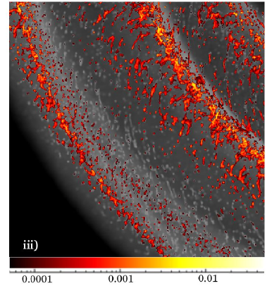
Whilst the distribution of hot gas changes little with time, the structure of the cold gas varies. Until approximately 60 Myr (Fig. 1i), the cold gas is fairly regularly distributed in small clumps across the section of disc, with an increased concentration in the spiral arms. Unlike the single-phase simulations, where the gas is clumpy due to the particle nature of the code, the warm phase here confines the cold gas into dense clumps. For the single-phase calculations, the clumpiness in the spiral arms is amplified with time by the dynamics of the shock (Dobbs et al., 2006). In these multi-phase calculations however, the spiral shock acts rather to organise these clumps into more coherent structures. These are perhaps more easily visible as the larger features shearing away from the spiral arms in Fig. 1ii and iii. By 220 Myr (Fig. 1iii) the 100 K spiral arm clumps have been sheared into thin filaments between the arms, whilst new structures are breaking away from the spiral arm.

Figure 2: The particle positions are shown for a section of the disc, assuming a Cartesian grid centred on the midpoint of the disc. The 2 phases are plotted, 100 K (blue) and $10^{4}$ K (red) after 100 Myr.

Figure 3: The distribution of mass as a function of gas density is shown after 100 Myr for the single (crosses) and multi-phase (100 K, squares and $10^{4}$ K gas, triangles) simulations. The nominal density for molecular clouds is n(H₂)=100 cm^-3 or $3\times 10^{-22}$ g cm^-3 (Williams et al., 2000).

3.2 Molecular gas density

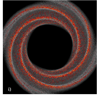
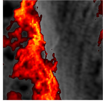
We show column density plots for the simulation after 100 Myr in Fig. 4. The column density of molecular hydrogen is highlighted in red. Fig. 4 shows more clearly the difference in structure of the cold gas in the single and multi-phase simulations, in particular by comparing Fig. 4 iv) and the equivalent frame of the single-phase simulation (Fig. 9 iv, Dobbs et al. 2006). The multi-phase gas is much more structured, with many smaller scale clumps visible. There are also small clumps of cold gas strewn across the inter-arm regions. Gas in the single-phase inter-arm regions is sheared into spurs and feathering (Dobbs & Bonnell, 2006), but individual clumps and structures are much more defined in the multi-phase medium. The cold gas assembles into longer, more coherent, very thin spurs in the inter-arm regions at later times in the multi-phase calculation (Fig. 1iii).

The molecular hydrogen corresponds to 12% of the total mass, i.e. 1.2 $\times 10^{8}$ M_⊙ and 24% of the cold gas. Most of the clumps of cold gas are over-plotted with the molecular hydrogen column density. The most striking difference between these results and those of Dobbs et al. (2006) (Fig. 9) is the greater amount of molecular gas. The fraction of molecular gas is approximately twice that of the single-phase simulation after 100 Myr. Unlike the single-phase calculations, the cold gas is confined by the pressure from the hot gas and remains more dense in the inter-arm regions. Consequently there is less photodissociation of H₂, and higher densities of molecular gas are produced between the spiral arms. As seen from Fig. 4 iii) and iv), the molecular gas does not become fully dissociated between the spiral arms, unlike the single-phase medium. The mass of molecular gas continues to rise throughout the multi-phase simulation, unlike the single-phase results, which peaked after about 100 Myr. As the gas is not fully dissociated between the arms, the total molecular gas density continues to increase after multiple spiral arm passages. By the end of the simulation the fraction of molecular gas appears to be converging to approximately 25 % of the total mass or equivalently 50 % of the 100 K gas ($2.5\times 10^{8}$ M_⊙). These figures are however dependent on the scale height used for the column densities of HI and H₂, which was assumed to be 100 pc (the scale height of the disc). Taking a scale height of 25 pc (comparable to the nearest B star from the Sun) reduces the total mass of H₂ by 30%.

Fig. 5 shows the density of the 100 K gas (total HI and predicted H₂), the predicted H₂ density and the $10^{4}$ K gas density as a function of azimuth. These are the average densities, calculated over a ring centred at 7.5 kpc, of width 200 pc and divided into 100 segments. This figure again shows the much higher density of H₂ in the inter-arm regions compared to the single-phase medium (Fig. 10, Dobbs et al. (2006)) with the density of H₂ now 1/10th of the total cold HI + H₂ gas in the inter-arm regions. The mass of molecular gas is now approximately 1/3 of the total mass of cold gas in the spiral arms, and 1/5 in the inter-arm regions. Fig. 5 further shows the difference in location of the shocks, as the density of the hot gas peaks at a lower azimuth than the cold gas.

Figure 4: Column density plots (g cm^-2) showing density of molecular hydrogen (red) against overall density (black and white). Length-scales of plots are i) 20 kpc $\times$ 20 kpc, ii) 10 kpc $\times$ 10 kpc, iii) 5 kpc $\times$ 5 kpc (-8.5 kpc $<x<$ -3.5 kpc, -8.5 kpc $<y<$ -3.5 kpc), iv) 3 kpc $\times$ 3 kpc (-6.5 kpc $<x<$ -3.5 kpc, -6.5 kpc $<y<$ -3.5 kpc). The xy-coordinates assume a Cartesian grid centred on the midpoint of the disc which remains fixed with time. Gas is flowing clockwise across the disc.

Figure 5: The average density is plotted (top) versus azimuth, calculated for a ring centred at 7.5 kpc ($\theta$ is measured clockwise round the disc). The density of the $10^{4}$ K gas (dotted), 100 K (dashed) (including HI and H₂) and H₂ (solid) are shown. The bottom figure shows the density of molecular hydrogen for individual particles (of similar phases) with time.

Figure 6: The typical time over which gas contains over a certain fraction of H₂ is shown in this figure. For each percentage of H₂, the average time is calculated from all particles which exceed that fraction of H₂ during each simulation. The average dynamical time for gas exceeding 90% H₂ is 5 Myr, increasing to 20 Myr for gas exceeding 10% H₂.

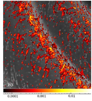Fig. 6 shows the typical timescale gas spends with different fractions of H₂. The average time for each fraction of H₂ is determined from the duration particles exceed that fraction of H₂ during each simulation. The typical time gas contains over 50% molecular hydrogen is around 40 Myr for the single phase simulation and 60 Myr for the multi-phase simulation. These times decrease to approximately 5 and 10 Myr for gas which contains over 90% molecular hydrogen. When a scale height of 25 pc is used, these timescales decrease by around 40%.

3.3 Inter-arm atomic and molecular gas

The distribution of mass with density is also shown specifically for the cold component in the inter-arm regions in Fig. 7. Clearly the inter-arm gas in the multi-phase simulation reaches densities over a magnitude higher than for the single phase simulation. From local simulations which include cooling, gas with densities $>10$ cm^-3 is found to be cold, i.e. 100-200 K or less (Fig. 1, Glover & Mac Low 2006a). We therefore expect a significant proportion of the cold gas entering the spiral arms to remain cold in a multi-phase medium. By contrast, for the single phase calculation, all the gas in the inter-arm regions is likely to increase in temperature above 100 K.

Figure 7: The distribution of mass as a function of gas density is shown for the cold gas in the inter-arm regions. The points are determined after 100 Myr for the single (crosses) and multi-phase (squares) simulations. Gas with densities above 10 cm^-3 (10^-23 g cm^-3) is expected to be cold (100-200 K) (Glover & Mac Low, 2006a).

For the multi-phase simulation, the density of the 100K gas (inclusive of H₂) is on average $1-2\times 10^{-23}$ g cm^-3 and $7\times 10^{-23}$ g cm^-3 for the inter-arm and spiral arm regions respectively (Fig. 5). Allen et al. (2004) find from models of photodissociaion regions (PDRs) that CO(1-0) emission is detected when the density is 10 cm${}^{-3}<n<10^{5}$ cm^-3. Whilst the spiral arm densities are high enough to be detected in CO, much of the inter-arm gas in our simulation lies below this regime and would be difficult to detect observationally. Kaufman et al. (1999) also show that the CO to H₂ conversion factor is roughly constant for a 100 cm^-3 cloud in a low UV field, providing the column density is $\gtrsim 4\times 10^{21}$ cm^-2 (comparable with the column density threshold used for our clump finding algorithms). Below these densities, or with a higher UV field, H₂ is significantly underestimated from CO observations since CO is dissociated more readily than H₂.

Fig. 4 further indicates that the column density of the inter-arm molecular gas is typically between $5\times 10^{-4}-10^{-3}$ g cm^-2. This is an order of magnitude less than the column densities of H₂ observed for HISA clouds which are associated with CO emission (Klaassen et al., 2005). However Klaassen et al. (2005) also examine HISA clouds where there is no CO emission, but infer, by means of radiative transfer techniques, column densities of H₂ for these clouds of around $10^{-3}$ g cm^-2. We postulate that the hot component of the ISM confines clouds of cold HI to sufficient densities to maintain a low level of H₂. The densities of these clouds imply that they will be largely undetected at present, but are high enough that the clouds are likely to be cold. We note however that the UV flux in these calculations is kept constant and we do not include feedback.

3.4 Resolution effects

We performed further simulations with 1 million (i.e. 500,000 cold gas particles for the multi-phase case) and 250,000 particles to investigate the effects of numerical resolution. The lower resolution results in lower peak gas densities since with fewer particles the spiral shock is less well resolved. Compared with Fig. 3., the peak densities for the cold gas decrease by a factor of 3 when 1 million particles are used, and a factor of 8 for 250,000 particles for the multiphase simulations. In the single phase simulations, the peak densities are similar for 1 million particles compared to 4 million, but decrease by a factor of 3 for 250,000 particles. Consequently the amount of molecular gas decreases with resolution, and only a few per cent of the gas is molecular when there are 250,000 particles.

For the multi-phase simulations, there is also a large decrease in the inter-arm densities of the gas, the peak densities shown on Fig. 7 decreasing by a factor of 10 in the lower resolution simulations. This reflects that these densities are dependent on the densities reached in the spiral arms and the confinement of this gas by the hot phase as it traverses the inter-arm regions. The average H₂ densities similarly decrease by a factor of 2-3 in the spiral arms compared with Fig. 5, and a factor of up to 10 in the inter-arm regions. There is little change in the the inter-arm densities for the single phase results (Fig. 7) where most gas leaving the spiral arms quickly diffuses to low densities. Apart from the change in the peak densities, the overall distribution of densities, as shown in Figures 3 and 7, is similar at different resolutions. However the peak densities, as well as molecular gas densities, represent lower limits both in the arm and inter-arm regions.

3.5 Structure in the cold gas

We now consider quantitatively the structure in the cold gas for the multi-phase medium, and compare this with the single-phase cold gas. We compare the properties of clumps from each simulation, using 2 clump finding algorithms. Both algorithms are grid based, assuming a 2D grid over the galactic disc. The first (hereafter CF1) selects clumps solely using a density threshold, whilst the second (hereafter CF2) uses neighbour lists to assign the most dense grid cells and their neighbours to clumps. For CF1, the density in each grid cell is calculated and all the cells above a certain density threshold are selected. Cells that are adjacent are grouped together and particles within these cells classed as a clump. CF2 was provided by Paul Clark and is based on the clump-find method of Williams et al. (1994). The SPH densities are first smoothed onto a 2D grid. The grid cells are then ordered by decreasing density. For each cell in turn, the cell and its neighbours (subsequently removed from the list) are identified as a clump, or assigned to a previously defined clump. Again a density threshold was set which removed low density cells. The properties of each clump are then calculated from the grid cells rather than the actual SPH particles. Since CF2 selects the most dense particles first, density peaks tend to be separated into separate clumps where they would otherwise constitute a single clump for CF1. In both cases we used the density of the molecular gas, which as seen from Fig. 4b largely reflects the underlying structure, and so we can compare the properties of these clumps with observed molecular clouds.

Figure 8: The top panel shows the distribution of clumps found using the clump-finding algorithm CF1 for a 1.2 by 1.2 kpc subsection of the disc after 100 Myr. The particles corresponding to the 100 K gas are plotted in dark blue, the $10^{4}$ gas is not shown. The particles in each clump are over-plotted in a different colour. The lower panel shows the corresponding column density image, using the same scale as Fig. 5 with molecular hydrogen overplotted in red.

Figure 9: The top panel shows the distribution of clumps found using the clump-finding algorithm CF1 for a 1.2 by 1.2 kpc subsection of the disc after 100 Myr. This is taken from the single-phase (50 K) simulation. The dark blue points show all the particles in the simulation, but the particles in clumps are overplotted in different colours. The lower panel shows the corresponding column density image, using the same scale as Fig. 4.

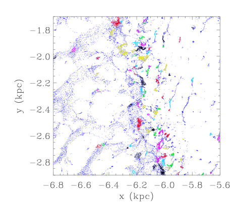
The clumps found using CF1 are displayed for the multi-phase (Fig. 8) and the single-phase medium (Fig. 9) for a subsection of the disc (the same section is shown in Fig. 2). Both these figures are taken after 100 Myr. The resolution of the grid for the algorithm is 5 pc, and the density threshold for each cell is 100 M_⊙, i.e. equivalent to a surface density of $9\times 10^{-4}$ g cm^-2. Each clump consists of at least 30 SPH particles (corresponding to a total hydrogen mass of 5000 M_⊙) which lie within cells above the density threshold. Clumps with fewer particles are discarded. We also show the corresponding column density plots indicating the molecular gas column density (Figs 8 and 9, lower).

There is a clear difference in structure of this section of the disc for the single and multi-phase gas. The multi-phase case shows many smaller clumps along the spiral arm, whilst the single-phase plot consists of 3 large clumps and several smaller clumps. Over the whole disc, there are 8383 clumps in the multi-phase calculation and 2066 in the single phase calculation. The clump finding algorithm also picks out several clumps in the inter-arm regions in the multi-phase simulation, whereas there are none for the single-phase results. These figures further show the general distribution of cold gas. In the multi-phase simulation, the cold gas occupies a much smaller filling factor, located in small dense clumps, particularly in the inter-arm regions. By contrast, in the single-phase case, the cold gas is much more uniform in the inter-arm regions. The second algorithm, CF2, generally produced smaller clumps, but with similar results.

3.6 Properties of molecular gas clumps

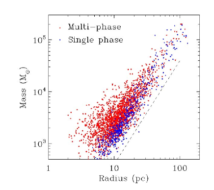
We now examine the properties of the clumps from the single and multi-phase simulations. The results shown use CF1, but we discuss any differences with the second clump-finding algorithm. Again only clumps with $>30$ particles are retained, and the clumps are located after 100 Myr. The mass and radii for the clumps from the 2 simulations are shown in Fig. 10. At later times the clump masses increase for the multi-phase simulation increase, as there is a higher fraction of H₂, while those of the single phase simulation are similar.

For both clump-finding algorithms, we take a column density threshold $9\times 10^{-4}$ g cm^-2. For CF1, this corresponded to taking a grid of resolution 5 pc and requiring that each cell contains at least 100 M_⊙ (of H₂). For CF2, we apply the same grid resolution, and a minimum column density of 0.001 g cm^-2 of H₂. With CF1, each clump corresponds to a group of SPH particles. The radii shown in Fig. 10 are determined by calculating the radius which contains 3/4 of the total clump mass, and thus the mass plotted is 3/4 of the total clump mass assigned by the particles. Using the full or 1/2 clump radii and masses merely shifts the distribution of clumps to higher or lower masses and radii. For CF2, we use the effective radius from the grid cells which make up each clump, i.e. $r_{eff}=\sqrt{Area/\pi}$ using the maximum extent of the $x$ and $y$ coordinates to calculate the area.

Fig. 10 shows the mass versus radii from the clumps found in the multi and single phase simulations from a quarter of the disc. The average smoothing length over all the particles is 30 pc, but reduces to 10 pc for particles above the cutoff density used for the clump-finding algorithm. There are far fewer clumps in the single-phase simulation - less than 1/3 of the multi-phase simulation. However there are comparatively more larger clouds, as also indicated by Figs 8 and 9. The total mass of the clumps in Fig. 10 for the single-phase simulation is $5.7\times 10^{6}$ M_⊙ compared to $1.4\times 10^{7}$ M_⊙ for the multi-phase simulation, over a quarter of the disc. The most massive clump after 100 Myr in both simulations was $\sim 3\times 10^{5}$ M_⊙, with a radius of 150 pc. For the multi-phase simulation, the fraction of molecular hydrogen increases with time, so after 200 Myr, the maximum cloud mass is $\sim 6\times 10^{5}$ M_⊙.

The clumps found using the second algorithm, CF2, follow a similar distribution to that shown on Fig. 10. However there is less scatter and fewer very massive clouds. The clumps from both simulations, and from both algorithms follow a $M\propto r^{2}$ dependence, implying the clouds have constant surface densities of $\sim 8$ M_⊙ pc^-2 ($2\times 10^{-3}$ g cm^-2). For comparison, the density criterion of 4 M_⊙ pc^-2 is also shown. The apparent constant surface density of the clumps is a consequence of the density threshold applied to find the clumps. Increasing the threshold 10 times moves the distribution of clumps to correspondingly smaller radii. The surface densities of molecular clouds from observational results (e.g. Heyer & Terebey 1998; Blitz et al. 2007) could similarly represent a selection effect based on the threshold antenna radiation temperature, $T_{R}^{*}$.

Since we do not include any feedback effects, most of the clumps are situated in the mid-plane of the disk, with average scale heights of $<10$ pc. However approximately 10% of the clouds, generally those of lower mass, have a centre of mass between 50 and 100 pc above or below the plane of the disk.

Figure 10: The mass and radius of the clumps are plotted using CF1 over a quarter of the disc. Lower mass clumps continue this distribution, but are not shown. The clumps are selected at 100 Myr. The dashed line indicates $\Sigma=9\times 10^{-4}$ g cm^-2 (4 M_⊙ pc^-2).

The resolution of most of the clumps was insufficient to calculate a velocity dispersion. However the better resolved clumps (with $>100$ particles) contain velocity dispersions of a few km s^-1. We also calculated the virial parameter,

$$\alpha_{G}=\frac{5\sigma^{2}r}{GM}.$$ (2)

for the clumps. In both simulations, most of the clumps are unbound. However the more massive clumps tend to be more bound, with $\alpha_{G}$ typically $<10$.

Fig. 11 shows the mass spectrum from the 2 simulations, for the total number of clouds found over the whole of the disc (of $>30$ particles) with CF1. Assuming a mass spectrum $dN/dM\propto M^{-\alpha}$, we find for the multi-phase simulation, $\alpha=2.35\pm 0.15$. The clumps from the single-phase simulation produce a much shallower spectrum, of $\alpha=1.6\pm 0.3$. At later times, the spectrum for the single-phase simulation is similar, although the spectrum for the multi-phase simulation becomes shallower, with $\alpha\sim 2.15$ after 200 Myr, since there are more larger clouds at later times. Using CF2, the larger clumps divide into smaller clumps which truncates the clump masses at $1.5\times 10^{5}$ M_⊙. Consequently the value of $\alpha$ increases to $\alpha\sim 3.3$ and $\alpha\sim 2.6$ for the multi and single-phase simulations respectively. The form of the mass spectrum thereby appears to depend on the details of the clump-finding algorithm. What can be concluded however is that the multi-phase medium produces a steeper mass spectrum and fewer high mass clouds. Observations indicate that $\alpha$ lies in the range $\alpha=1.5-1.8$ (Solomon et al., 1987; Heyer & Terebey, 1998) for the Galaxy and up to $\alpha=2.5$ for external galaxies (Blitz et al., 2007).

Fig. 12 shows the clump mass spectra for the multi-phase simulation with 6 million, 1 million and 250,000 particles. The clumps are again found using CF1, using the same column density threshold (hence the clumps lie within the distribution in Fig. 10), but increasing the grid-size for the clump-finding algorithm. All the clumps contain $>$ 30 particles. The slope becomes shallower as the resolution decreases and with 1 million particles the total amount of H₂ is significantly reduced to 10%. At lower resolutions, less massive mass clouds cannot be detected, although the upper mass is not significantly reduced compared to the higher resolution simulations. For single phase calculations the slope of the spectrum was the same for 4 and 1 million particles, but shallower for 250,000 particles. In summary, we stress that the results presented here should be taken as lower limits on the fraction of molecular gas present, both in the spiral arms and in the interarm regions.

3.6.1 Inter-arm and spiral arm molecular clouds

As mentioned previously, the multi-phase simulation produces a much greater degree of inter-arm molecular gas and a few of the clumps in Fig. 8 are located in the inter-arm regions. We show the distribution of molecular clouds over the whole of the disc, using CF1, in Fig. 13. There are a significant number of clouds in the inter-arm regions, especially in the inner regions of the disc where the spiral arms are closer together. For the outer parts of the disc, the inter-arm clouds tend to be situated on the edge of spiral arms. We estimate the ratio of inter-arm to arm clouds is approximately 1:7 (decreasing to 1:10 for the 1 million particle simulation, and no inter-arm clouds at lower resolution). The distribution of clouds and the inter-arm ratio is very similar for the second clump-finding algorithm. By contrast, for the single phase simulation, the clouds all lie along the spiral arms. Consequently observational-style plots of the molecular clouds over a range of longitudes (Dobbs et al. 2006 Fig. 14 & 15) show a greater degree of scatter in the inter-arm regions.

We also considered the number of more massive clouds in the inter-arm and arm regions. Approximately 3% of inter-arm clouds were $>10^{4}$ M_⊙ compared to 6% of clouds in the spiral arms. The cloud mass spectra for clouds located in the spiral arms and inter-arm regions are displayed in Fig. 14. The spectrum for the spiral arm clouds is very similar to the spectrum for the total number of clouds, although slightly shallower with $\alpha=2.25\pm 0.15$. The spectrum for the inter-arm clouds however is much steeper with $\alpha=2.9\pm 0.4$, and a cut off in mass at around $3\times 10^{4}$ M_⊙.

Figure 11: The clump mass spectrum is shown for clumps from the multi-phase simulation (solid) and the 50 K simulation (dotted). Both are determined after 100 Myr and use CF1. The masses indicated are the mass of H₂. The imposed limit of 30 particles corresponds to a total (HI and H₂) mass of approximately $10^{3.5}$ M_⊙. Allowing that the actual mass of H₂ is a fraction of the total, the resolution limit corresponds with the peak of the distributions, below which the sample is incomplete and the number of clumps rapidly drops off. The slope corresponds to $dN/dM\propto M^{-2.35}$ for clumps from the multi-phase simulation compared to $dN/dM\propto M^{-1.6}$ for the single phase results.

The number of inter-arm clouds is sensitive to the photodissociation rate, so these figures only provide a rough indication. The photodissociation rate may be lower in the inter-arm regions, increasing the number of inter-arm clouds. On the other hand, the photodissociation rate will be higher where massive star formation occurs, which with the effects of feedback may disrupt molecular gas clouds before they enter the inter-arm regions.

Figure 12: The clump mass spectrum is shown for the multi-phase simulation using different resolutions. The clump mass is the mass of H₂. The total number of particles is indicated for each simulation.

Figure 13: The distribution of clumps is displayed for the multi-phase simulation, using CF1 after 100 Myr.

Figure 14: The clump mass spectrum is shown for the clumps in the spiral arms (dotted) and inter-arm regions (solid) from the multi-phase simulation. The clumps are selected at 100 Myr, and again the minimum (total) mass resolution of the clumps is $10^{3.5}$ M_⊙.

4 Conclusions

We have performed hydrodynamic simulations of a multi-phase medium subject to a spiral potential. We find that including hot gas in addition to cold leads to higher densities in the cold gas. Consequently the amount of molecular gas increases in the disc, with 1/4 of the cold gas molecular after 100 Myr, approximately double that of corresponding single phase calculations. This fraction further increases with time. The increase in H₂ is most striking in the inter-arm regions, with molecular clouds surviving into the inter-arm regions without being destroyed by photodissociation, although both feedback, and heating and cooling of the gas are neglected. For the whole disc, approximately 1/7 of the molecular clouds lie in the inter-arm regions, but this ratio decreases with radius as the separation of the spiral arms increases. The spiral arm H₂ densities increase to values comparable with average GMC densities, whilst the typical inter-arm densities are below those detected with CO. We therefore propose that a multi-phase medium predicts a population of cold clouds of HI and molecular hydrogen, which are currently undetected.

The multi-phase simulations also show more structure in the cold gas, with smaller clumps present compared to the single phase calculations. Consequently the mass spectrum is steeper for the multi-phase clouds, although the value of the exponent is found to depend on the clump-finding method. The maximum cloud mass is $6\times 10^{5}$ M_⊙ in the multi-phase simulation, comparable to GMCs in M33 (Engargiola et al., 2003), but an order of magnitude lower than the most massive GMCs observed in the Milky Way. The free-fall times for the molecular clouds are esimated to range from 5 Myr, when over 90% of the gas is molecular, to 20 Myr when over 10% of the gas is molecular. The lifetimes of the clouds are estimated to be 20 Myr for when over 90% of the gas is molecular, and 80 Myr when over 10% of the gas is molecular, both of which correspond to roughly 4 free-fall times (5 Myr for $>$ 90% and 20 Myr for $>$ 10% H₂).

The main factor which will affect these results is the inclusion of feedback, particularly in determining how much molecular gas is retained in the ISM following star formation. This may lead to less inter-arm molecular gas, but would also introduce the possibility of triggered molecular cloud formation in the inter-arm regions. Furthermore, using lower scale heights to determine the photodissociation rate could also reduce the amount of H₂.. Thirdly we do not include heating and cooling of the different phases. Rather we have assumed a fixed composition of the ISM to approximately agree with observations. Previous simulations of the ISM with heating and cooling show that a cold phase of gas is sustained, with 20-30% of gas (Audit & Hennebelle, 2005) to 60% or more (Wada & Norman, 2001; Piontek & Ostriker, 2005) in the cold regime. We leave a more complete treatment of the thermodynamics of the ISM and spiral shocks for future work.

References

- Allen et al. (2004) Allen R. J., Heaton H. I., Kaufman M. J., 2004, ApJ, 608, 314
- Audit & Hennebelle (2005) Audit E., Hennebelle P., 2005, A&A, 433, 1
- Bate et al. (2003) Bate M. R., Bonnell I. A., Bromm V., 2003, MNRAS, 339, 577
- Benz (1990) Benz W., 1990, in in Buchler J.R., ed., Numerical Modelling of Nonlinear Stellar Pulsations Problems and Prospects, p269. Smooth Particle Hydrodynamics - a Review, Kluwer, Dordrecht
- Bergin et al. (2004) Bergin E. A., Hartmann L. W., Raymond J. C., Ballesteros-Paredes J., 2004, ApJ, 612, 921
- Blitz et al. (2007) Blitz L., Fukui Y., Kawamura A., Leroy A., Mizuno N., Rosolowsky E., 2007, in Reipurth B., Jewitt D., Keil K., eds, Protostars and Planets V Giant Molecular Clouds in Local Group Galaxies. pp 81–96
- Bonnell et al. (2006) Bonnell I. A., Dobbs C. L., Robitaille T. P., Pringle J. E., 2006, MNRAS, 365, 37
- Bonnell et al. (2007) Bonnell I. A., Larson R. B., Zinnecker H., 2007, in Reipurth B., Jewitt D., Keil K., eds, Protostars and Planets V The Origin of the Initial Mass Function. pp 149–164
- Cox (2005) Cox D. P., 2005, ARA&A, 43, 337
- Cox & Gómez (2002) Cox D. P., Gómez G. C., 2002, ApJS, 142, 261
- Dobbs & Bonnell (2006) Dobbs C. L., Bonnell I. A., 2006, MNRAS, 367, 873
- Dobbs et al. (2006) Dobbs C. L., Bonnell I. A., Pringle J. E., 2006, MNRAS, 371, 1663
- Engargiola et al. (2003) Engargiola G., Plambeck R. L., Rosolowsky E., Blitz L., 2003, ApJS, 149, 343
- Gibson et al. (2005) Gibson S. J., Taylor A. R., Higgs L. A., Brunt C. M., Dewdney P. E., 2005, ApJ, 626, 195
- Gibson et al. (2006) Gibson S. J., Taylor A. R., Stil J. M., Brunt C. M., Kavars D. W., Dickey J. M., 2006, in IAU Symposium Cold HI in Turbulent Eddies and Galactic Spiral Shocks
- Gittins & Clarke (2004) Gittins D. M., Clarke C. J., 2004, MNRAS, 349, 909
- Glover & Mac Low (2006a) Glover S. C. O., Mac Low M. M., 2006a, astro-ph/0605120
- Glover & Mac Low (2006b) Glover S. C. O., Mac Low M. M., 2006b, astro-ph/0605121
- Heitsch et al. (2005) Heitsch F., Burkert A., Hartmann L. W., Slyz A. D., Devriendt J. E. G., 2005, ApJL, 633, L113
- Heyer & Terebey (1998) Heyer M. H., Terebey S., 1998, ApJ, 502, 265
- Kaufman et al. (1999) Kaufman M. J., Wolfire M. G., Hollenbach D. J., Luhman M. L., 1999, ApJ, 527, 795
- Kim & Ostriker (2002) Kim W., Ostriker E. C., 2002, ApJ, 570, 132
- Kim et al. (2003) Kim W.-T., Ostriker E. C., Stone J. M., 2003, ApJ, 599, 1157
- Klaassen et al. (2005) Klaassen P. D., Plume R., Gibson S. J., Taylor A. R., Brunt C. M., 2005, ApJ, 631, 1001
- Le Petit et al. (2004) Le Petit F., Roueff E., Herbst E., 2004, A&A, 417, 993
- Lequeux et al. (1993) Lequeux J., Allen R. J., Guilloteau S., 1993, A&A, 280, L23
- Mac Low & Klessen (2004) Mac Low M.-M., Klessen R. S., 2004, Reviews of Modern Physics, 76, 125
- Monaghan (1992) Monaghan J. J., 1992, ARA&A, 30, 543
- Monaghan & Lattanzio (1985) Monaghan J. J., Lattanzio J. C., 1985, A&A, 149, 135
- Ostriker et al. (2001) Ostriker E. C., Stone J. M., Gammie C. F., 2001, ApJ, 546, 980
- Piontek & Ostriker (2005) Piontek R. A., Ostriker E. C., 2005, ApJ, 629, 849
- Pringle et al. (2001) Pringle J. E., Allen R. J., Lubow S. H., 2001, MNRAS, 327, 663
- Solomon et al. (1987) Solomon P. M., Rivolo A. R., Barrett J., Yahil A., 1987, ApJ, 319, 730
- Thacker et al. (2000) Thacker R. J., Tittley E. R., Pearce F. R., Couchman H. M. P., Thomas P. A., 2000, MNRAS, 319, 619
- Vazquez-Semadeni et al. (2006) Vazquez-Semadeni E., Gomez G. C., Jappsen A. K., Ballesteros-Paredes J., Gonzalez R. F., Klessen R. S., 2006, astro-ph/0608375
- Vazquez-Semadeni et al. (1995) Vazquez-Semadeni E., Passot T., Pouquet A., 1995, ApJ, 441, 702
- Vogel et al. (1988) Vogel S. N., Kulkarni S. R., Scoville N. Z., 1988, Nature, 334, 402
- Wada & Koda (2004) Wada K., Koda J., 2004, MNRAS, 349, 270
- Wada & Norman (1999) Wada K., Norman C. A., 1999, ApJL, 516, L13
- Wada & Norman (2001) Wada K., Norman C. A., 2001, ApJ, 547, 172
- Williams et al. (2000) Williams J. P., Blitz L., McKee C. F., 2000, Protostars and Planets IV, pp 97–+
- Williams et al. (1994) Williams J. P., de Geus E. J., Blitz L., 1994, ApJ, 428, 693
- Wolfire et al. (2003) Wolfire M. G., McKee C. F., Hollenbach D., Tielens A. G. G. M., 2003, ApJ, 587, 278