SHOCKS AND COLD FRONTS IN GALAXY CLUSTERS
Abstract
The currently operating X-ray imaging observatories provide us with an exquisitely detailed view of the Megaparsec-scale plasma atmospheres in nearby galaxy clusters. At , the Chandra’s 1′′ angular resolution corresponds to linear resolution of less than a kiloparsec, which is smaller than some interesting linear scales in the intracluster plasma. This enables us to study the previously unseen hydrodynamic phenomena in clusters: classic bow shocks driven by the infalling subclusters, and the unanticipated “cold fronts,” or sharp contact discontinuities between regions of gas with different entropies. The ubiquitous cold fronts are found in mergers as well as around the central density peaks in “relaxed” clusters. They are caused by motion of cool, dense gas clouds in the ambient higher-entropy gas. These clouds are either remnants of the infalling subclusters, or the displaced gas from the cluster’s own cool cores.
Both shock fronts and cold fronts provide novel tools to study the intracluster plasma on microscopic and cluster-wide scales, where the dark matter gravity, thermal pressure, magnetic fields, and ultrarelativistic particles are at play. In particular, these discontinuities provide the only way to measure the gas bulk velocities in the plane of the sky. The observed temperature jumps at cold fronts require that thermal conduction across the fronts is strongly suppressed. Furthermore, the width of the density jump in the best-studied cold front is smaller than the Coulomb mean free path for the plasma particles. These findings show that transport processes in the intracluster plasma can easily be suppressed. Cold fronts also appear less prone to hydrodynamic instabilities than expected, hinting at the formation of a parallel magnetic field layer via magnetic draping. This may make it difficult to mix different gas phases during a merger. A sharp electron temperature jump across the best-studied shock front has shown that the electron-proton equilibration timescale is much shorter than the collisional timescale; a faster mechanism has to be present. To our knowledge, this test is the first of its kind for any astrophysical plasma. We attempt a systematic review of these and other results obtained so far (experimental and numerical), and mention some avenues for further studies.
keywords:
galaxies: clusters: general – X-rays: galaxies: clusters – hydrodynamicsUpdated version of an article to appear in Physics Reports astro-ph/0701821
1 INTRODUCTION
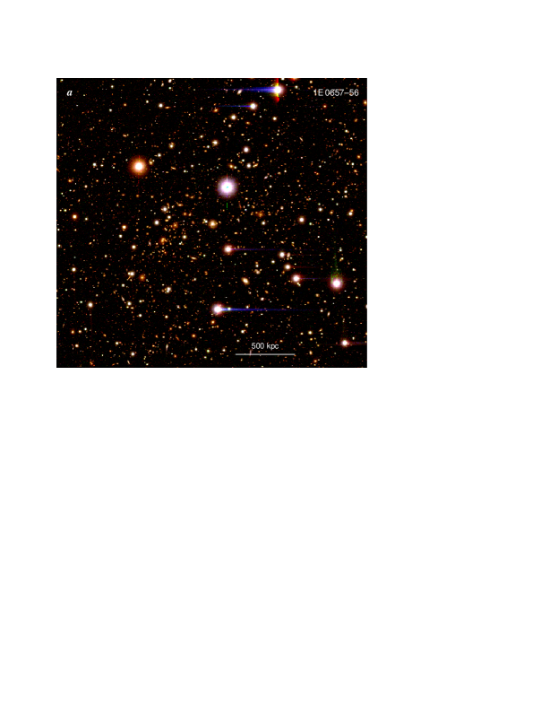
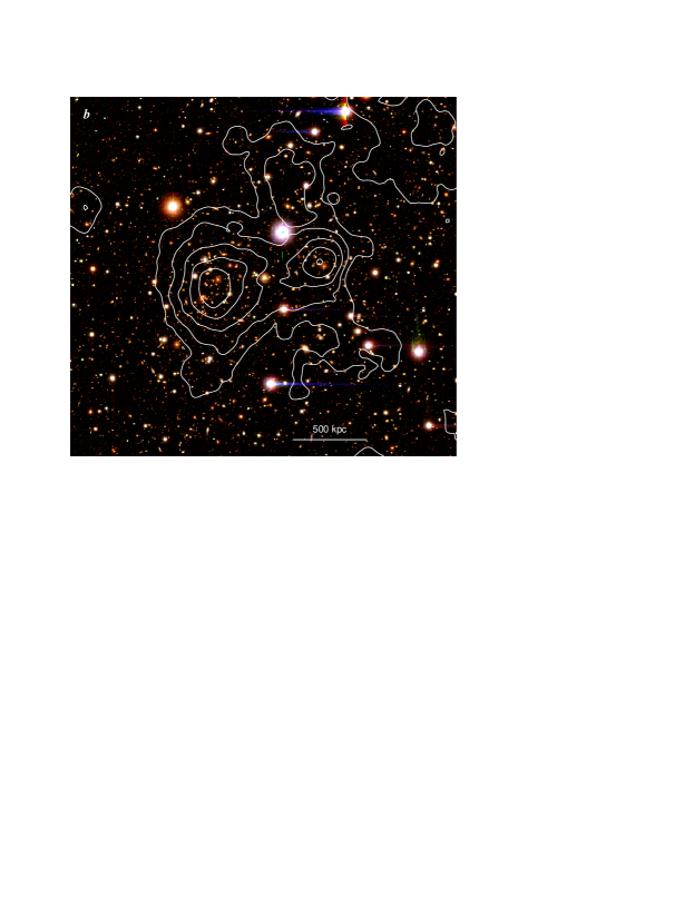
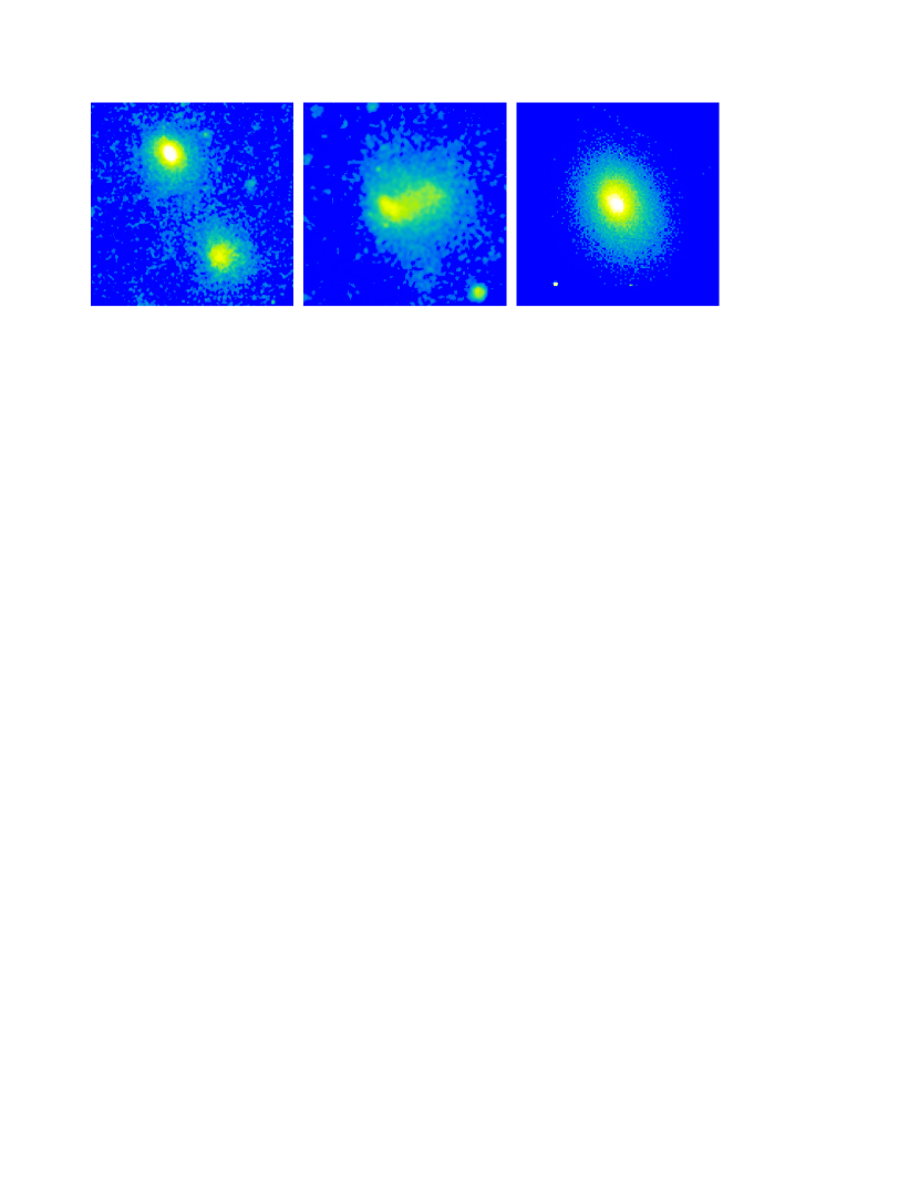
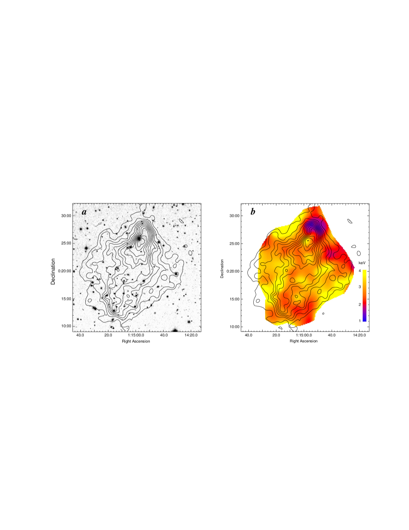
Clusters of galaxies are the most massive gravitationally bound objects in the Universe. They include hundreds of galaxies within a radius of 1–2 Mpc (e.g., Abell 1958). Dispersions of the member galaxy redshifts indicate that the gravitational potential of the cluster is much deeper than can be created by the total mass of its galaxies, revealing the presence of smoothly distributed dark matter (Zwicky 1937). Its nature is still unknown, except that it is probably cold and collisionless. At present, its distribution can be directly mapped using the gravitational lensing distortion that it introduces to the images of distant background galaxies (e.g., Bartelmann & Schneider 2001). In Fig. 1, panels (a) and (b), we show an optical image of the field containing a relatively distant cluster 1E 0657–56, and a map of its total projected mass derived from lensing. Within the radius covered by the image, this cluster has a mass of about ( g), of which only 1–3% is stellar mass in the member galaxies.
X-ray observations showed that intergalactic space in clusters is filled with hot plasma (Kellogg et al. 1972; Forman et al. 1972; Mitchell et al. 1976; Serlemitsos et al. 1977). It is the second most massive cluster component, and their dominant baryonic component. A theoretical and observational review of this plasma and other cluster topics can be found in Sarazin (1988). Here we summarize the basics which will be needed in the sections below.
The intracluster medium (ICM) has temperatures K ( keV) and particle number densities steeply declining from cm-3 near the centers to cm-3 in the outskirts. It consists of fully ionized hydrogen and helium plus traces of highly ionized heavier elements at about a third of their solar abundances, increasing to around solar at the centers. It emits X-rays mostly via thermal bremsstrahlung. At densities and temperatures typical for the ICM, the ionization equilibrium timescale is very short. The electron-ion equilibration timescale via Coulomb collisions is generally shorter than the age of the cluster, so can be assumed in most cluster regions, except perhaps in the low-density outskirts and at shock fronts (and probably even there, as will be seen in §4.5). The spectral density of the X-ray continuum emission at energy from such a plasma is
| (1) |
where is the effective Gaunt factor, which includes all continuum mechanisms and depends weakly on , and ion abundances (e.g., Gronenschild & Mewe 1978; Rybicki & Lightman 1979). On top of this continuum, there is line emission, discussed, e.g., by Mewe & Gronenschild (1981). The timescale of radiative cooling of the ICM is generally very long, longer than the cluster age, with the exception of small, dense central regions. Thus, nonradiative approximation is applicable to all the phenomena discussed in this review.
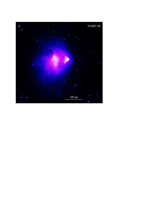
The ICM is optically thin for X-rays for all densities encountered in clusters (except for the possible resonant scattering at energies of strong emission lines in the dense central regions; Gilfanov, Sunyaev, & Churazov 1987). An X-ray telescope can thus map the ICM density and electron temperature in projection. The current X-ray imaging instruments are sensitive mostly to X-rays with keV. From eq. (1), an X-ray image of a hot cluster at is essentially a map of the projected . In Fig. 1c, we show an X-ray image of 1E 0657–56 as an example. This highly disturbed cluster has one of the hottest and most X-ray luminous plasma halos (with keV and a bolometric luminosity of erg s-1), and will feature in several sections below.
The electron temperature, , averaged along the line of sight, can be determined from the shape of the continuum component, and sometimes from the relative intensities of emission lines, using an X-ray spectrum collected from a spatial region of interest. The ion temperature, , cannot be directly measured at present. In principle, it can be determined from thermal broadening of the emission lines, but this requires an energy resolution of a calorimeter. Because of the strong dependence of on , it is often possible to “deproject” the ICM temperature and density in three dimensions under reasonable assumptions about the symmetry of the whole cluster or within a certain region of the cluster. In such a way, the mass of the hot plasma can be determined for many clusters whose gas atmospheres are spherically symmetric. It is found to comprise 5–15% of the total mass, several times more than the stellar mass in galaxies (e.g., Allen et al. 2002; Vikhlinin et al. 2006).
If a cluster is undisturbed by collisions with other clusters for a sufficient time, its dark matter distribution should acquire a centrally peaked, slightly ellipsoidal, symmetric shape. After several sound crossing times (of order yr), the ICM comes to hydrostatic equilibrium in the cluster gravitational potential , so that the pressure of the ICM and its mass density satisfy the equation . For a spherically symmetric cluster, and assuming that the intracluster plasma can be described as ideal gas, it can be written as
| (2) |
where is the total mass of the cluster enclosed within the radius , is the gas temperature at that radius, and is the mean atomic weight of the plasma particles. That is, by measuring radial distributions of the gas temperature and density, one can derive the cluster total mass (Bahcall & Sarazin 1977; Sarazin 1988). This method of measuring the cluster masses is independent of, and complementary to, those using galaxy velocity dispersions and gravitational lensing. Unlike the lensing mass measurement, it works only for clusters in equilibrium; however, it is less affected by the line-of-sight projections. For those clusters where a comparison is possible, different total mass measurement methods usually agree to within a factor of 2.
Cluster masses are interesting because the ratio of the baryonic mass (ICM plus stars) to dark matter mass for a cluster should be close to the average for the Universe as a whole, which enables some powerful cosmological tests (e.g., White et al. 1993; Allen et al. 2004). Furthermore, the number density of clusters as a function of mass and its evolution with redshift depend sensitively on cosmological parameters, which is the basis for another class of tests (e.g., Sunyaev 1971; Press & Schechter 1974; Eke, Cole, & Frenk 1996; Henry 1997; Vikhlinin et al. 2003). Hot electrons in the ICM also introduce a distortion in the spectrum of the Cosmic Microwave Background (CMB), which at mm turns clusters into negative radio “sources” (Sunyaev & Zeldovich 1972). By comparing the Sunyaev-Zeldovich decrement and the X-ray brightness and temperature, one can derive absolute distances to the clusters and, again, use them for a cosmological test (Silk & White 1978). The best estimates of the cluster baryonic and total masses currently come from the X-ray data. To rely on them for cosmological studies, we have to understand in detail the physical processes in the ICM, how well the quantities required for those tests can be determined from the X-ray images and spectra, and how valid are the underlying assumptions about the ICM. This has been the main motivation for the studies discussed in this review.
Clusters form via gravitational infall and mergers of smaller mass concentrations, as illustrated by a time sequence in Fig. 2. Such mergers are the most energetic events in the Universe since the Big Bang, with the total kinetic energy of the colliding subclusters reaching ergs (Markevitch, Sarazin, & Vikhlinin 1999a). In the course of a merger, a significant portion of this energy, that carried by the gas, is dissipated (on a Gyr timescale) by shocks and turbulence. Eventually, the gas heats to a temperature that approximately corresponds to the depth of the newly formed gravitational potential well.
A fraction of the merger energy may be channeled into the acceleration of ultrarelativistic particles and amplification of magnetic fields. These nonthermal components manifest themselves most clearly in the radio band. Polarized radio sources located inside and behind clusters are known to exhibit Faraday rotation, which is caused by magnetic fields in the ICM. In the radial range Mpc (outside the dense central regions often affected by the central AGN), the field strengths are in the range G (with different measurement methods giving somewhat diverging values; for a review see, e.g., Carilli & Taylor 2002). For such fields and the typical ICM temperatures, gyroradii for thermal electrons and protons are of order cm and cm, respectively, many orders of magnitude smaller than the particle collisional mean free paths ( cm). The plasma electric conductivity is very high and the magnetic field is frozen in. For typical ICM densities and a G field, the Alfvén velocity is km s-1, much lower than the typical thermal sound speeds km s-1. Thus, the plasma is “hot” in the sense that the ratio of thermal pressure to magnetic pressure , except in special places which will be discussed in §3.3.3. This means, among other things, that the magnetic pressure contribution is negligible for the hydrostatic mass determination using eq. (2).
The magnetic field is tangled, with coherence scales of order 10 kpc (Carilli & Taylor 2002). This suppresses collisional thermal conduction on scales greater than this linear scale, by a large factor that depends on the exact structure of the field (Chandran & Cowley 1998; Narayan & Medvedev 2001). As a result, plasma with temperature gradients (for example, created by a merger) comes to pressure equilibrium much faster than those gradients dissipate (e.g., Markevitch et al. 2003a). Indeed, we are yet to find a cluster without spatial temperature variations.
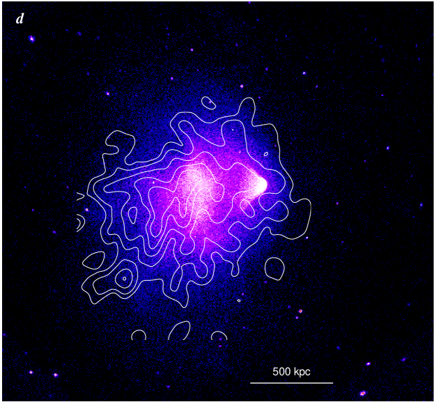
Merging clusters often exhibit faint radio halos, such as that shown in Fig. 1d (for a review see, e.g., Feretti 2002; radio halos are not to be confused with the more localized radio “relics” of different origin). The radio emission at GHz is produced by synchrotron radiation of ultrarelativistic electrons with Lorentz factor in a microgauss magnetic field. These relativistic electrons coexist with thermal ICM, bound to it by the magnetic field. Their exact origin is uncertain; one possibility is acceleration by merger turbulence (for a review see, e.g., Brunetti 2003; we will touch on this in §4.6). Relativistic electrons also produce X-ray emission by inverse Compton (IC) scattering of the CMB photons. A detection of such nonthermal emission at keV (where thermal bremsstrahlung falls off exponentially with energy) was reported for some clusters (e.g., Fusco-Femiano et al. 2005 and references therein). The energy density in the relativistic electrons should be of the order of the magnetic pressure and thus negligible compared to thermal pressure of the ICM. However, it was suggested that the currently unobservable relativistic protons that may accompany them can have a significant energy density (Völk et al. 1996 and later works).
A part of our review will deal with hydrodynamic phenomena near the cluster centers, and a brief description of these rather special regions will be helpful. One of the models for the radial dark matter density distribution, widely used until recently, is the King (1966) profile, . It has a flat core in the center with typical sizes kpc (see, e.g., Sarazin 1988 for a motivation for this model). An isothermal gas in hydrostatic equilibrium within such a potential also has a flat density core (Cavaliere & Fusco-Femiano 1976). This is an adequate description of the observed gas density profiles for about 1/3 of the clusters. However, most clusters exhibit sharp central gas density peaks (e.g., Jones & Forman 1984; Peres et al. 1998). Coincidentally, Navarro, Frenk & White (1997, hereafter NFW) found that density profiles of equilibrium clusters in their cosmological Cold Dark Matter simulations can be approximated by a functional form . Its dark matter density cusp in the center corresponds to a finite, but sharp density peak of the gas in equilibrium. The NFW model is a good description for the total mass profiles derived from the X-ray data for such centrally peaked clusters (e.g., Markevitch et al. 1999b; Nevalainen et al. 2001; Allen, Schmidt, & Fabian 2001; Pointecouteau, Arnaud, & Pratt 2005; Vikhlinin et al. 2006). These clusters usually have relatively undisturbed ICM (see, e.g., the last panel in Fig. 2) and a giant elliptical galaxy in the center (a cD galaxy) which marks the dark matter density peak. Within kpc of this peak, the ICM temperature declines sharply toward the center (e.g., Fukazawa et al. 1994; Kaastra et al. 2004; Sanderson, Ponman, & O’Sullivan 2006), while the gas density increases, along with the relative abundance of heavy elements in the gas. This creates a rather distinct central region of low-entropy gas. Outside this region, the radial temperature gradient reverses and declines outward, but the entropy continues to increase, so on the whole, the clusters are convectively stable. The high central gas densities correspond to X-ray radiative cooling times shorter than the cluster ages (a few Gyr). This gave rise to a “cooling flow” scenario, in which central regions of such peaked clusters are thermally unstable. Recent data indicate that there has to be a process that partially compensates for the radiative cooling; for a recent review see, e.g., Peterson & Fabian (2006). We will use the term “cooling flow” to signify this region that encloses the observed gas density and temperature peaks (positive and negative, respectively), without any particular physical model in mind.
Gas density and temperature distributions in clusters have been studied extensively by all imaging X-ray observatories (e.g., by Einstein, Forman & Jones 1982; Jones & Forman 1999; ROSAT, Briel, Henry, & Boehringer 1992; Henry & Briel 1995; Peres et al. 1998; Vikhlinin, Forman, & Jones 1997, 1999; ASCA, Fukazawa et al. 1994; Honda et al. 1996; Markevitch et al. 1996a, 1998; SAX, Nevalainen et al. 2001; De Grandi & Molendi 2002; XMM, Arnaud et al. 2001; Briel, Finoguenov, & Henry 2004; Piffaretti et al. 2005). Temperature maps proved to be more difficult to obtain than maps of the gas density, but the currently operating XMM and Chandra observatories have the right combination of spectroscopic and imaging capabilities to derive them with a good linear resolution for a large number of clusters at a range of redshifts. At , Chandra’s 1′′ angular resolution, the best among the X-ray observatories, corresponds to linear scales kpc. This is less than the typical collisional mean free path in the ICM or a typical galaxy size, and provides an exquisitely detailed view of the physical processes in the cluster Megaparsec-sized gas halos. With Chandra, we are able to see the classic bow shocks driven by infalling subclusters, as well as “cold fronts” — unexpected sharp features of a different nature. While XMM can measure temperatures with a higher statistical accuracy, its angular resolution is not sufficient to see these sharp features in full detail, so our review of these two phenomena will be based almost exclusively on the Chandra results.
Chandra’s main detector, ACIS, is sensitive in the 0.5–8 keV energy band, with a peak sensitivity between 1–2 keV, and has a FWHM energy resolution of eV for extended sources, sufficient to disentangle emission lines in the uncrowded cluster X-ray spectra, but far from that needed to resolve the line Doppler widths. A Chandra overview can be found, e.g., in Weisskopf et al. (2002). Uncertainties of the cluster gas temperatures from typical Chandra exposures are limited by the photon counting statistics, while uncertainties of the gas densities are usually limited by the assumed three-dimensional geometry of a cluster. Physical quantities below are given for a spatially flat cosmology with , , and km sMpc-1 (unless the dependence on is given explicitly via a factor km sMpc-1).
2 COLD FRONTS
Those interested primarily in physics that can be learned from this recently found phenomenon may read §2.1, which gives a general description of cold fronts, then skip the rest of this chapter (which discusses the various kinds of cold fronts and their origin and evolution based on hydrodynamic simulations), and go directly to §3.
2.1 Cold fronts in mergers
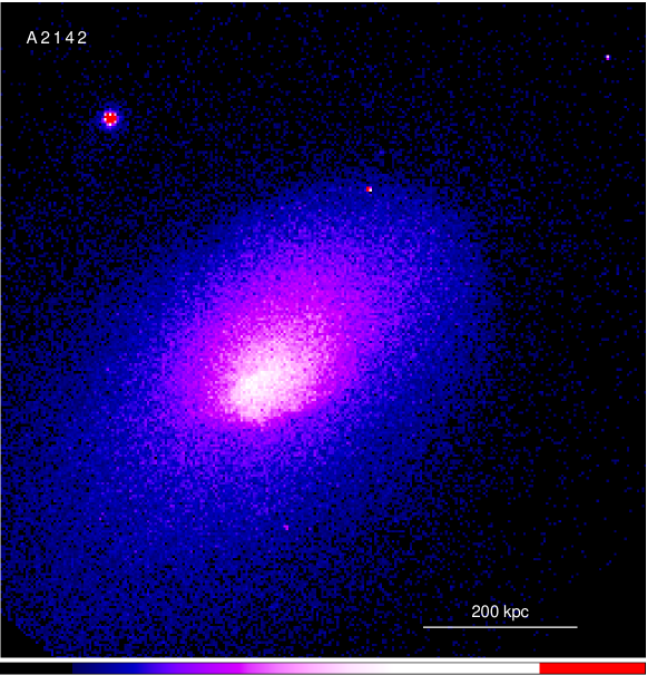
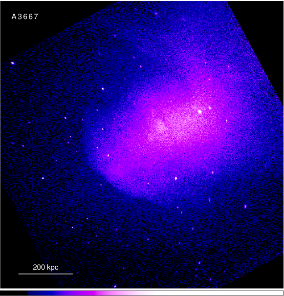
Among the first Chandra cluster results was a discovery of “cold fronts” in merging clusters A2142 and A3667 (Markevitch et al. 2000, hereafter M00; Vikhlinin, Markevitch, & Murray 2001b, hereafter V01). Figure 3 shows ACIS images of the central regions of A2142 and A3667, which show prominent sharp X-ray brightness edges. The edge in A3667 was previously seen in a lower-resolution ROSAT image (Markevitch et al. 1999a), and at the time, we interpreted it as a shock front, even though the crude ASCA temperature map did not entirely support this explanation.
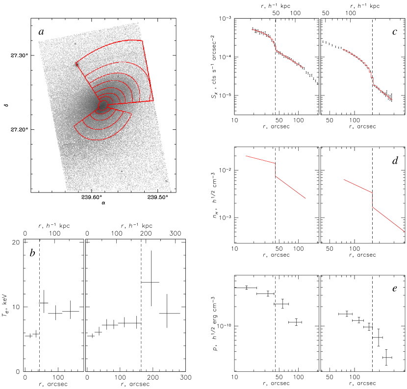
If these features were shocks, the gas on the denser, downstream side of the density jump would have to be hotter than that on the upstream side. With ROSAT and ASCA, we could not derive sufficiently accurate gas temperature profiles across such edges. Chandra provided this capability for the first time, so now we can easily test this hypothesis. The Chandra radial X-ray brightness and temperature profiles across the two edges in A2142 are shown in Fig. 4 (from M00). They were extracted in sectors shown in panel (a). Both brightness profiles have a characteristic shape corresponding to a projection of an abrupt, spherical (within a certain sector) jump of the gas density. Best-fit radial density models of such a shape are shown in panel (d), and their projections are overlaid on the data as histograms in panel (c) — they provide a very good fit. Since there is no way of knowing the exact three-dimensional geometry of the edge, for such fits we have to assume that the curvature of the discontinuity surface along the line of sight is the same as in the sky plane. To ensure the consistency with this assumption, it is important that the radial profiles and the three-dimensional model for the gas inside the discontinuity are centered at the center of curvature of the front, which is often offset from the cluster center. At the same time, the model of the outer, “undisturbed” gas may need to be centered elsewhere (e.g., the cluster centroid).
Panel (b) in Fig. 4 shows the gas temperature profiles across the edges. For a shock discontinuity, the Rankine–Hugoniot jump conditions directly relate the gas density jump, , and the temperature jump, , where indices 0 and 1 denote quantities before and after the shock (e.g., Landau & Lifshitz 1959, §89):
| (3) |
or, conversely,
| (4) |
where we denoted ; here is the adiabatic index for monoatomic gas.
For the observed density jump and a presumably post-shock temperature keV observed inside the NW edge in A2142, one would expect to find a keV gas in front of the shock. This sign of the temperature change is opposite to that observed across the edge — the temperature in the less dense gas outside the edge is in fact higher than that inside (Fig. 4b). The same is true for the smaller edge in A2142, as well as the one in A3667 (V01; see also Briel, Finoguenov, & Henry 2004), ruling out the shock interpretation.
What are these sharp edges then? One hint is given by the gas pressure profiles across the edges (simply the product of the best-fit density models and the measured temperatures; Fig. 4e), which show that there is approximate pressure equilibrium across the density discontinuity (as opposed to a large pressure jump expected in a shock front). One also notes a smooth, comet-like shape of the NW edge in A2142, which looks as if the ambient gas flows around it. Given this evidence, we proposed (M00) that these features are contact discontinuities at the boundaries of the gas clouds moving sub- or transonically through a hotter and less dense surrounding gas — or “cold fronts”, as V01 have termed a similar feature in A3667.111We were certainly influenced by the Burns (1998) review, which compared the gasdynamic phenomena in cluster mergers with “stormy weather”. The term “cold front” has since been commonly adopted to denote either the discontinuity itself, or the discontinuity and the gas cloud behind it; which of these two is usually clear from the context. Strictly speaking, a contact discontinuity implies continuous pressure and velocity between the gas phases, but a cold front often has a discontinuous tangential velocity, when the dense gas cloud is moving.
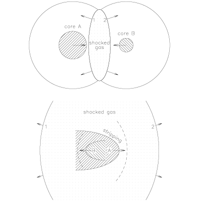
In the particular scenario that was envisioned for A2142 in M00, these dense gas clouds are remnants of the cool cores of the two merging subclusters that have survived shocks and mixing of a merger (which would have to have a nonzero impact parameter to avoid complete destruction of the less dense NW core). They are observed after the passage of the point of minimum separation and presently moving apart. The hotter, rarefied gas beyond the NW edge can be the result of shock heating of the outer atmospheres of the two colliding subclusters, as schematically shown in Fig. 5. In this scenario, the less dense outer subcluster gas has been stopped by the collision shock, while the dense cores (or, more precisely, regions of the subclusters where the pressure exceeded that of the shocked gas in front of them, which prevented the shock from penetrating them) continued to move ahead through the shocked gas, pulled along by their host dark matter clumps.
With the benefit of a more recent, longer Chandra observation of A2142, and having seen images of numerous other clusters as well as hydrodynamic simulations, we now think that the M00 scenario is not correct. Instead, it seems more likely that A2142 is a cluster with a sloshing cool core (as first pointed out by Tittley & Henriksen 2005), a phenomenon that was discovered later and which will be discussed in §2.3. However, the physical interpretation of the X-ray edges as contact discontinuities between moving gases of different entropies still holds — the only difference is the origin of the two gas phases in contact (either from different subclusters or from different radii in the same cluster). At the same time, the scenario proposed in M00 is realized in a number of other merging clusters. Two particularly striking examples are the textbook merger 1E 0657–56 and an elliptical galaxy NGC 1401 in the Fornax cluster, although each of these systems exhibits only one cold front. In both objects, there is an independent (i.e., non X-ray) evidence of a distinct infalling subcluster that hosts the gas cloud with a cold front. In Fornax, a cold front forms at the interface between the atmosphere of the infalling galaxy NGC 1404 seen in the optical image, and the hotter cluster gas (Fig. 6; Machacek et al. 2005). In 1E 0657–56, a mass map derived from the gravitational lensing data reveals a dark matter subcluster, which is also seen as a concentration of galaxies in the optical image (Fig. 1ab; Clowe, Gonzalez, & Markevitch 2004; Clowe et al. 2006). Its X-ray image (Fig. 1c) shows a bright “bullet” of gas moving westward, apparently pulled along by the smaller dark matter subcluster. Because of ram pressure, the bullet lags behind the collisionless dark matter clump (Fig. 38, which will be discussed in §4.7).
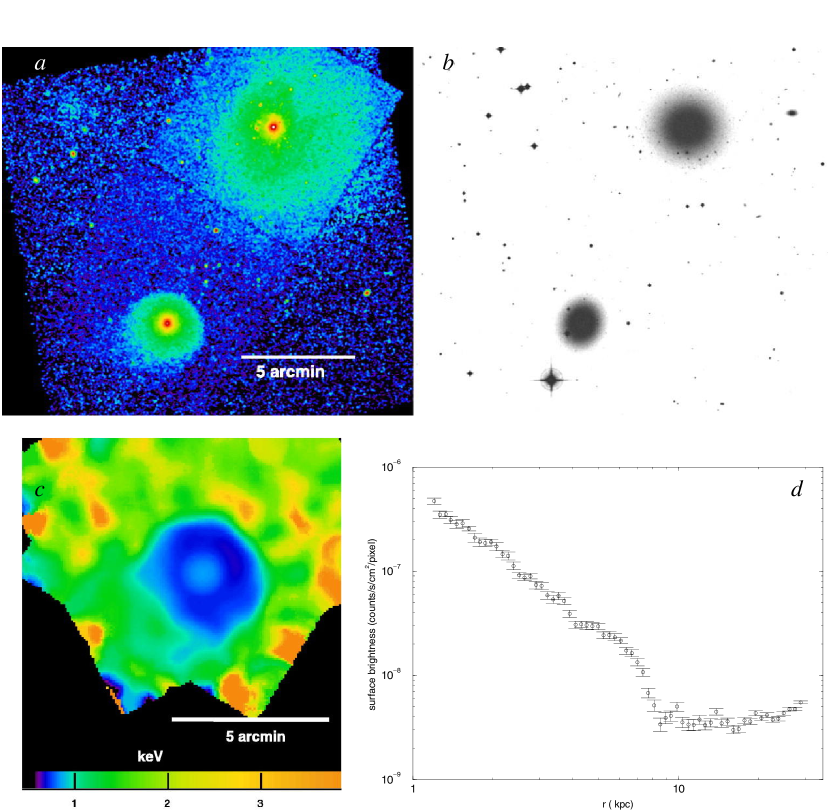
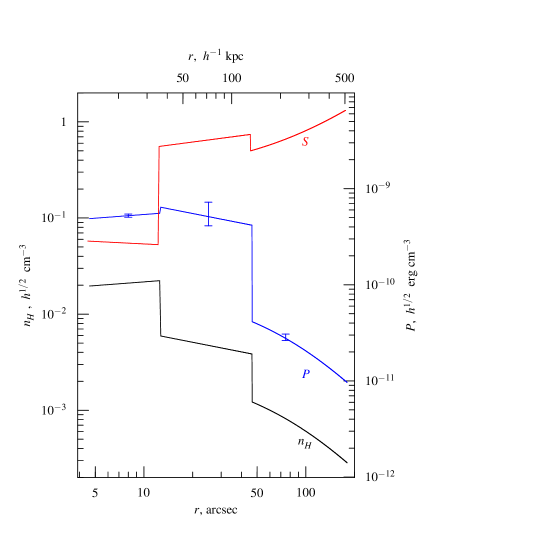
The gas bullet in 1E 0657–56 has developed a sharp edge at its western side, which is a cold front. Ahead of it is a genuine bow shock (a faint blue-black edge in Fig. 1c), confirmed by the temperature profile (Markevitch et al. 2002, hereafter M02; §4.2 below). It is instructive to look at the radial profiles of the gas density, thermal pressure and specific entropy derived in a narrow sector crossing both these edge features (Fig. 7). The two discontinuities have density jumps of similar amplitudes (a factor of 3). As expected, the pressure has a big jump at the shock, but is nearly continuous in comparison at the cold front. In broad terms, thermal pressure in the cool gas behind a moving cold front should be in balance with the thermal plus ram pressure of the gas flowing around it. For a substantially supersonic motion (this shock has , see §4.2), the gas flow between the bow shock and the driving body is very subsonic. So the ram pressure component is small compared to thermal pressure, hence the near-continuity of thermal pressure (a more detailed picture will be presented in §3.1). The entropy, on the other hand, shows only a small increase at the shock (as expected for this relatively weak shock), but a big drop at the cold front. This is because in the past, the bullet apparently used to be a cooling flow (M02). The merger brought this region of low-entropy gas in direct contact with the high-entropy gas from the cluster outskirts. These are the characteristic features of all cold fronts, regardless of the exact origin of the two gas phases in contact.
In addition to the examples mentioned above, prominent if less clear-cut cold fronts have been observed in a large number of other clusters (e.g., RXJ 1720+26, Mazzotta et al. 2001; A2256, Sun et al. 2002; A85, Kempner, Sarazin, & Ricker 2002; A2034, Kempner, Sarazin, & Markevitch 2003; A496, Dupke & White 2003; A754, Markevitch et al. 2003a; A2319, O’Hara, Mohr, & Guerrero 2004, Govoni et al. 2004, hereafter G04; A168, Hallman & Markevitch 2004; A2204, Sanders, Fabian, & Taylor 2005). Many of such features have been observed at smaller linear scales in the cool dense gas near the cluster centers, which we will separate (somewhat artificially) into a class of their own (§2.3).
2.2 Origin and evolution of merger cold fronts
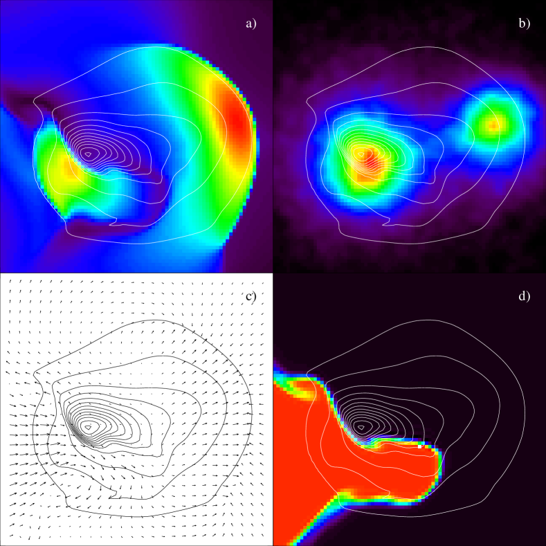
Since their discovery, cold fronts in merging clusters have been looked for, and found, in hydrodynamic simulations with cosmological initial conditions (e.g., Nagai & Kravtsov 2003; Onuora, Kay & Thomas 2003; Bialek, Evrard, & Mohr 2002; Mathis et al. 2005). Several other recent works used idealized 2D or 3D merger simulations to model the effects of ram-pressure stripping of a substructure moving through the ICM (e.g., Heinz et al. 2003; Acreman et al. 2003; Takizawa 2005; Ascasibar & Markevitch 2006, hereafter A06). In fact, these features could already be seen in earlier simulations of idealized mergers, such as those of Roettiger, Loken, & Burns (1997). For example, an obvious cold front is seen in a merger simulated by Roettiger, Stone, & Mushotzky (1998), although they have not yet heard of this term then and therefore concentrated on other aspects of their result. We present their simulated cluster in Fig. 8, which shows maps of the gas temperature and velocity, dark matter density and X-ray brightness for two subclusters right after a core passage. Panel (d) shows the fraction of gas that initially belonged to each subcluster; a cold front is the boundary between the two gases that did not mix. The linear resolution of this and other contemporary simulations (as well as most of the present-day ones) was limited to kpc, which is why they could not predict that these interfaces would be so strikingly sharp in real clusters when looked at with Chandra. Nevertheless, keeping this limitation in mind, we can use these and newer simulations to clarify the origin and evolution of cold fronts.
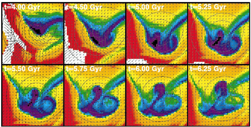
Indeed, simulations show that when two subclusters collide, the outer regions of their gas halos are shocked and stopped, while the lower-entropy gas cores are often dense enough to resist the penetration of shocks and stay attached to their host dark matter subclusters. This can be seen in a time sequence for an interesting region selected from a cosmological simulation (Fig. 9, from Mathis et al. 2005). The upper panels show two similar dark matter subclusters colliding and passing nearly through each other (the pericenter passage occurs between and ). In lower panels, we see how the gas between the clusters is first heated via compression and then by shocks, which propagate outwards after the pericentric passage. At and later, we see the emergence of two cold fronts, which are the boundaries of the unstripped remnants of the two former subcluster gas cores. This is pretty much the picture proposed in M00 (Fig. 5) and seen in other simulations (e.g., Nagai & Kravtsov 2003).
Ram pressure stripping
Ram pressure of the ambient gas first pushes these gas remnants out of the gravitational potential wells of their respective subclusters. Depending on the depth of the well, the density of the ambient gas and the merger velocity, the ram pressure may or may not succeed in stripping the subcluster gas completely, as shown in Fig. 10. As long as it does not succeed, the cool dense gas core is dragged along by the gravity of the subcluster, initially slightly lagging behind its dark matter peak. The ambient shocked gas flows around it, separated by a sharp contact discontinuity. This is the stage at which we observe the bullet subcluster in 1E 0657–56 (Fig. 38).
Ram pressure slingshot
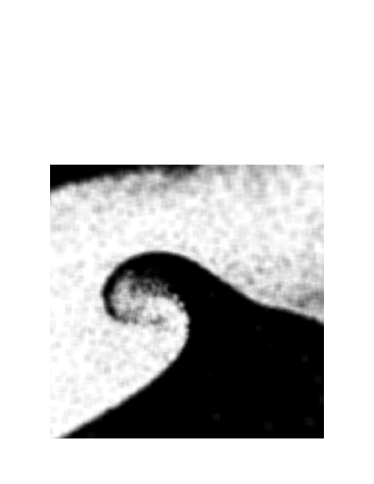
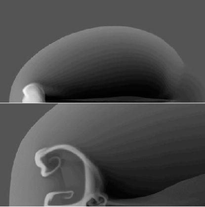
For a subcluster that has managed to retain its cool core through the pericenter passage where the ram pressure was the highest, an interesting thing happens at a later stage. As the subcluster moves away from the pericenter and slows down, it also enters the region with a lower density of the ambient gas, and the ram pressure on the cool cores drops very rapidly (). As a result, the cool gas rebounds and overtakes the dark matter core as if in a slingshot. The forward region of the cool core moves away from the gravitational potential minimum which kept it at high pressure, expands adiabatically and cools, further enhancing the temperature contrast at the cold front (as noted by Bialek et al. 2002). This is what we observe in A168 (Fig. 11, from Hallman & Markevitch 2004) — instead of lagging behind, a cold front in that cluster is located “ahead” of the most likely center of the northern subcluster (a giant galaxy seen in the optical image). This process is also seen at late stages of the Mathis et al. simulations (note the crescent-shaped cool regions appearing in the last panel in Fig. 9). This “ram pressure slingshot” is further illustrated in Fig. 12 (taken from A06), which shows a small subcluster passing near the center of a larger cluster. The corresponding black and white panels show the gas that initially belonged to each of the subclusters. At first, ram pressure exerted by the dense subcluster gas pushes the main cluster core far away from the dark matter peak. However, as soon as the subcluster passes, that ram pressure drops, and the main cluster gas (black) rebounds under the effect of gravity and unbalanced thermal pressure behind the front, overshooting the center. Note that in both panels, the boundary of the main cluster core is a cold front, but at the latter moment, the temperature contrast at the front is enhanced by adiabatic expansion. Interestingly, a gas temperature map for A3667 obtained with XMM (Heinz et al. 2003; Briel et al. 2004), which has sufficient statistical accuracy to show the small-scale detail, shows that the coolest gas is located right along the cold front, suggesting that the front in A3667 is at this late, “slingshot” stage of its evolution. (Another possibility is that the cool spot in A3667 is a remnant of a cooling flow-like initial temperature distribution.)
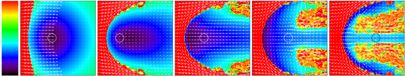
There may be an additional effect that helps to enhance the temperature contrast at the cold fronts. Heinz et al. (2003) used idealized two-dimensional hydrodynamic simulation to model the evolution of a contact discontinuity between a uniform wind flowing around a cool, initially isothermal (and therefore, with the specific entropy declining toward the center), cluster-like gas cloud in a stationary gravitational potential of the underlying dark matter halo. The initially planar discontinuity has developed into a spheroidal cold front with a flow of ambient (post-shock) gas around it (Fig. 13). The gas halo in this simulation is first displaced from the potential minimum along the direction of the wind (panel 2), but then the central, lowest-entropy gas rebounds, overshoots the potential minimum (as in the ram-pressure slingshot described above) and starts flowing toward the cold front (panel 3). At the same time, the ambient flow around the contact discontinuity has generated a shear layer in which the Kelvin-Helmholtz (KH) instabilities drag the cool gas located just under the surface of the front to the sides and away from the tip (panel 3 and later). This is in addition to the usual flattening and sideways expansion of a dense gas sphere subjected to a wind. If occurs in real clusters, this “circulation” may help the low-entropy gas located deeper under the surface to reach the tip.

2.3 Cold fronts in cluster cool cores
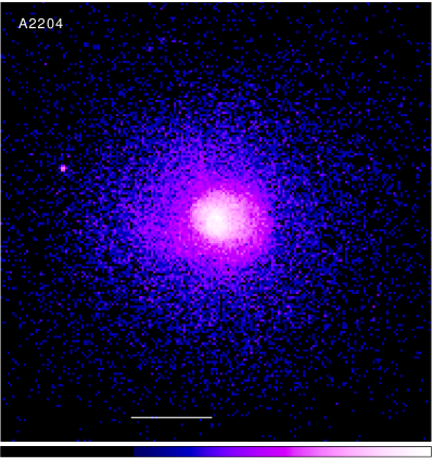
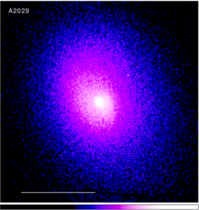
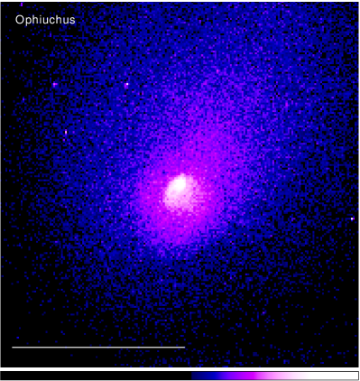
When the subclusters merge, one does expect to see vigorous gas flows, including moving remnants of the subcluster cores which give rise to cold fronts. Surprisingly, though, cold fronts are also observed near the centers of most “cooling flow” clusters, many of which are relaxed and show little or no signs of recent merging (e.g., Mazzotta et al. 2001; Markevitch, Vikhlinin, & Mazzotta 2001, hereafter M01; Mazzotta, Edge, & Markevitch 2003; Churazov et al. 2003; Dupke & White 2003; Sanders et al. 2005). These fronts are typically more subtle in terms of the density jump than those in mergers, and occur on smaller linear scales close to the center ( kpc), with their arcs usually curved around the central gas density peak. There are often several such arcs at different radii around the density peak. Cooling flow clusters by definition have a sharp temperature decline and an accompanying density increase toward the center (that is, a sharp decline of specific entropy). The edges are seen inside or on the boundaries of this cool central region. This is a very common variety of the cold fronts; we found them in more than a half of the cooling flow clusters (Markevitch, Vikhlinin, & Forman 2003b). Given the projection, this means that most, if not all, cooling flow clusters may have one or several such fronts. Some of the clusters with such fronts are shown in Fig. 14. One of them is A2029, which on scales kpc is the most undisturbed cluster known (e.g., Buote & Tsai 1996). As in mergers, cold fronts in these clusters must indicate gas motion; however, the moving gas clearly does not belong to any infalling subcluster.


We studied such a feature in A1795 — another one of the most-relaxed nearby clusters (Buote & Tsai 1996) — and showed that the gas forming a cold front is not in hydrostatic equilibrium in the cluster gravitational potential (M01). Figure 15 (reproduced from M01) shows radial profiles of X-ray brightness and gas temperature in the sector of A1795 that contains the cold front, along with the best-fit gas density model and the resulting pressure profile. The brightness edge is barely noticeable (and would certainly go undetected without the Chandra’s arcsecond resolution) and corresponds to a density jump by only a factor of 1.3 (for comparison, in the more prominent merger cold fronts discussed in §2.1, the density jumps by factors 2–5). The pressure profile turns out to be almost exactly continuous, leaving little or no room for a relative gas motion, since the ram pressure from such a motion would cause the inner thermal pressure to be higher compared to that on the outside (beyond a small stagnation region; see §3.1 below). Thus the inner and outer gases appear very nearly at rest and in pressure equilibrium. Therefore, one might expect them to be in hydrostatic equilibrium in the cluster gravitational potential.
For a spherically symmetric cluster in hydrostatic equilibrium, one can derive the cluster total (mostly dark matter) mass from the above radial profiles of the gas density and temperature using eq. (2). The resulting mass profile in the immediate vicinity of the edge in A1795 is shown in Fig. 15e. The profile reveals an unphysical discontinuity by a factor of 2 at the front. For comparison, a similar analysis was performed using a sector on the opposite side from the center, which has smooth distributions of gas density and temperature. The total mass profile derived using that sector is overlaid as a dashed line. If the gas around the cluster center were in hydrostatic equilibrium, both sectors would measure the same enclosed cluster mass. Indeed, outside the edge radius, the masses derived from the two opposite sectors agree, strongly suggesting that the gas immediately outside the edge is indeed near hydrostatic equilibrium. But the gas inside the edge is not — even though there is pressure equilibrium between the two sides of the edge.
Such an unphysical mass discontinuity at the cold front was first reported by Mazzotta et al. (2001) for the cluster RXJ 1720+26, which is similarly relaxed on large scales. Although the statistical accuracy of the available temperature profile was not sufficient to exclude a significant bulk velocity of the cool gas, the situation appears similar to A1795.
2.3.1 Gas sloshing
Given the above evidence, we proposed (M01) that the low-entropy gas in the A1795 core is “sloshing” in the central potential well (Fig. 16). The observed edge delineates a parcel of cool gas that has moved from the cluster center and is currently near the point of maximum displacement, where it has zero velocity but nonzero centripetal acceleration. In agreement with this scheme, there is a kpc cool gas filament extending from the cD galaxy in the center of A1795 toward this cold front (Fabian et al. 2001), suggesting that the bulk of the central gas has indeed been flowing around the cD galaxy (which most probably sits in the gravitational potential minimum). Such an oscillating gas parcel would not be in hydrostatic equilibrium with the potential — instead, the gas distribution would reflect the reduced gravity force in the accelerating reference frame, resulting in the above unphysical mass underestimate. M01 made an estimate of this acceleration from the apparent mass jump , assuming that the gas outside the edge is hydrostatic: cm s-2 or , where is the radius of the edge, which is a sensible number for an oscillation on this linear scale. More recent detailed simulations (A06, see below) have shown that this picture is somewhat oversimplified, but the physics in it is correct.
In M01 we suggested that this subsonic sloshing of the cluster’s own cool, dense central gas in the gravitational potential well may be the result of a disturbance of the central potential by past subcluster infall. There are striking examples suggesting that this is the case at least in some clusters (Fig. 17). Alternatively, one can imagine some off-center disturbance in the gas from the activity of the central AGN; AGNs blowing bubbles in the intracluster gas are observed in many cooling flow clusters (e.g., Fabian et al. 2000; Nulsen et al. 2005). However, the absence of any visible merger or AGN disturbance in the X-ray images of two of the most undisturbed clusters, A2029 and A1795, presented an apparent difficulty, which has motivated some of the numerical studies reviewed below.
2.3.2 Simulations of gas sloshing
Several simulation works addressed the possibility that mergers can create cold fronts in the cluster centers. Churazov et al. (2003) and Fujita, Matsumoto & Wada (2004) used 2D simulations to show that a weak shock or acoustic wave propagating toward the center of a cooling flow cluster can displace the cool gas from the gravitational potential well and cause gas sloshing, giving rise to cold fronts. On the other hand, Tittley & Henriksen (2005), using mergers extracted from a cosmological simulation, suggested that cold fronts in the cores arise when the gas peak is dragged along as the dark matter peak oscillates around the cluster centroid because of a gravitational disturbance from a merging subcluster.
The most detailed simulation that addressed the specific question of whether a merger can generate cold fronts in the cores, but no visible disturbance elsewhere, was presented by A06. They found that sloshing is indeed easily set off by any minor merger and can persist for gigayears, producing concentric cold fronts just as those observed. The only necessary (and obvious) condition for their formation is a steep radial entropy drop in the gas peak, such as that present in all cooling flows. Most interestingly, fronts form even if the infalling subcluster has not had any gas during core passage. This may occur if the gas was stripped early in the merger, leaving a clump of only the dark matter and galaxies. It is mergers with such gasless clumps that can set the central cool dense gas in motion, while leaving no other long-lived visible traces in X-rays.
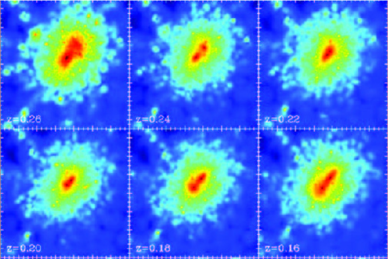
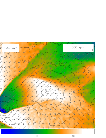
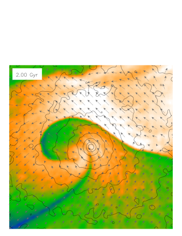
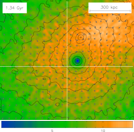
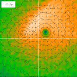
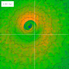
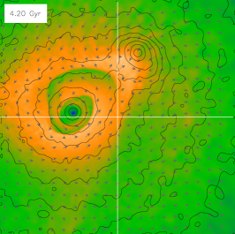
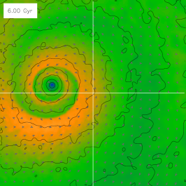
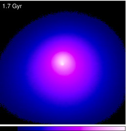
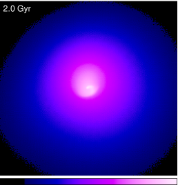
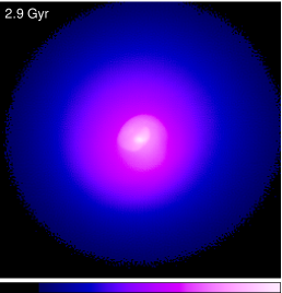
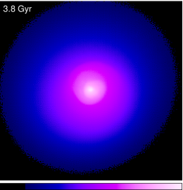
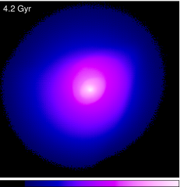
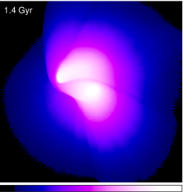
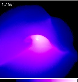
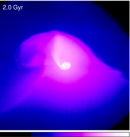
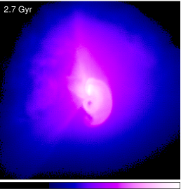
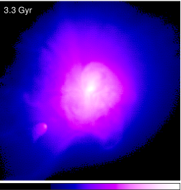
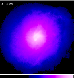
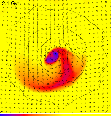
Figure 18 (from A06) shows a time sequence from a simulated merger with the dark matter-only subcluster whose mass is 1/5 of that of the main cluster and which falls in with a nonzero impact parameter (or angular momentum). The figure shows how the subcluster makes two passes, around 1.4 Gyr and 4.2 Gyr from the start of the simulation run. During the first pass, the gravitational disturbance created by the subhalo causes the density peak of the main cluster (DM and gas together) to swing along a spiral trajectory relative to the center of mass of the main cluster (white cross in Fig. 18). The gas and DM peaks feel the same gravity force and initially start moving together toward the subcluster. However, during the core passage, the direction of this motion quickly changes, leading to a rapid change of the ram-pressure force exerted on the gas peak. Mainly as a result of this change, the cool gas core shoots away from the potential minimum in a ram-pressure slingshot similar to the one described above in §2.2. Subsequently, the densest gas turns around and starts falling back toward the minimum of the gravitational potential (a cuspy NWF mass profile has a well-defined sharp potential minimum). It then starts sloshing around the DM peak and generating long-lived cold fronts, as will be discussed below.
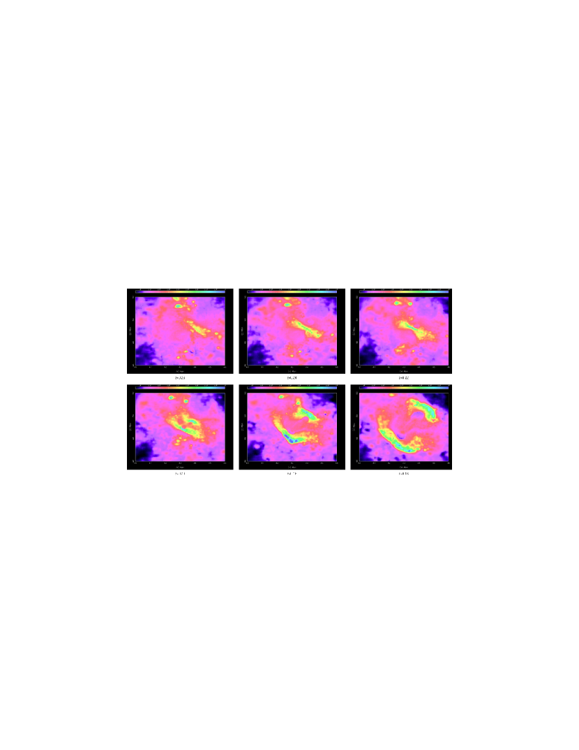
Mock X-ray images of this simulated merger (Fig. 19) show these cold fronts quite clearly, at the same time exhibiting very little disturbance on the cluster-wide scale. The exception is several brief periods when the DM satellite crosses the cluster and generates a subtle conical wake (first and last panels in Fig. 19), but the subcluster spends most of the orbiting time in the outskirts. This simulation looks very much like the most relaxed cooling-flow clusters in the real world, such as A2029 and A1795.
For comparison, Fig. 20 shows mock X-ray images from a simulation of a similar merger, but with the gas subcluster. Hydrodynamic effects of the collision of two gas clouds are now overwhelming and the gas is disturbed on all scales for a long time. Sloshing and central cold fronts are generated, too — in fact, sloshing occurs on a wider scale, because the initial displacement caused by the subcluster shock and stripped gas is much stronger than that caused by a swinging motion of the DM peak. There are many real clusters that look similar to this simulation.
The emergence of multiple cold fronts
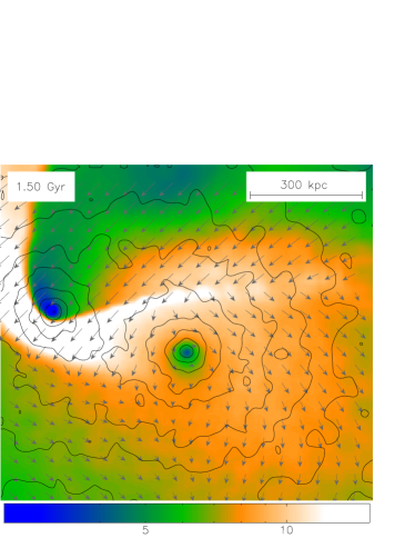
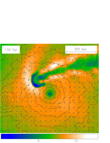
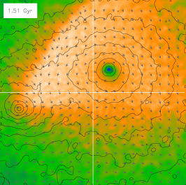
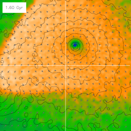
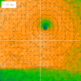
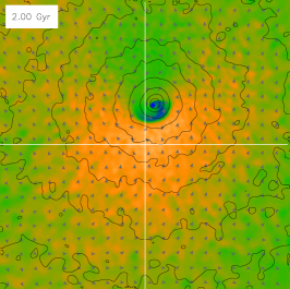
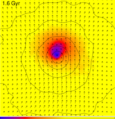
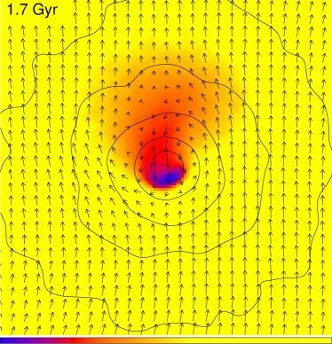
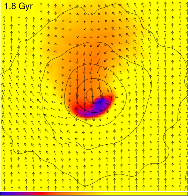
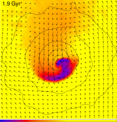
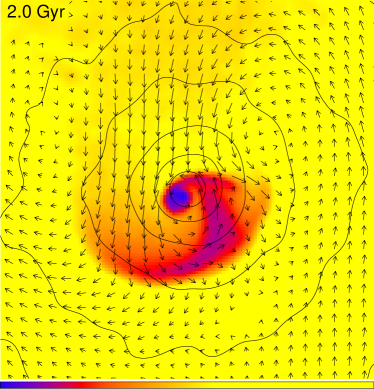
Let us now examine in details how the sloshing central gas gives rise to cold fronts. Figure 21 presents a zoomed-in view of the gas temperature and velocity field from the A06 simulation of a merger with the gasless subcluster. The dark matter peak has a cuspy NFW density profile, and the initial gas density and temperature profiles are similar to those observed in cooling flow clusters, so this is what should happen in clusters such as A2029. The figure shows several snapshots following the initial displacement of the gas density peak from the central potential dip. The displaced cool gas expands adiabatically as it is carried further out by the flow of the surrounding gas (the orange plume above the center in the 1.6–1.7 Gyr panels of Fig. 21). However, in a process similar to the onset of a Rayleigh-Taylor (RT) instability, the densest, coolest gas turns around and starts sinking towards the minimum of the gravitational potential, as seen most clearly in the 1.6 Gyr and again in the 1.8 Gyr snapshots. The coolest gas overshoots the center at 1.7 Gyr and, subjected to ram pressure from the gas on the opposite side still moving in the opposite direction, eventually spreads into a characteristic mushroom head with velocity eddies (von Karman vortices) at the sides. This is a classic structure seen in numeric and real-life experiments involving a gas jet flowing through a less dense gas (for cluster-related works see, e.g., Heinz et al. 2003, our Fig. 13; Takizawa 2005). The mushroom head forms where the dense gas is slowed by the ambient ram pressure and spreads sideways into the regions of lower pressure created by the flow of the ambient gas around a blunt obstacle (Bernoulli’s law). The front edges of these mushroom heads are sharp discontinuities, as confirmed by a detailed look at these structures (A06). We will discuss how exactly they arise in §2.3.3 below.
At 1.8 Gyr, one can see how the inner side of the first mushroom head sprouts a new RT tongue — the densest, lowest-entropy gas separates and again starts sinking toward the potential minimum (compare this, e.g., with a structure in the center of the Ophiuchus cluster in Fig. 14). Meanwhile, the rest of the gas in the first mushroom head continues to move outwards, expanding adiabatically as it moves into the lower-pressure regions of the cluster, and roughly delineating the equipotential surfaces. The process repeats itself, and these mushroom heads are generated on progressively smaller linear scales. Sloshing of the densest gas that is closest to the center occurs with a smaller period and amplitude than that of the gas initially at greater radii (the reason is explained in Churazov et al. 2003). It is this period difference that eventually brings into contact the gas phases that initially were at different off-center distances and had different entropies (recall that a cooling flow gas profile has a sharp radial entropy gradient).
The picture is qualitatively similar even if there is no cooling flow-like temperature drop — as long as there is entropy gradient. Ricker & Sarazin (2001) simulated a merger in an isothermal cluster with a cuspy potential, which shows the formation of similar multiple mushroom heads (Fig. 22). The specific entropy declines toward the center, but less steeply than in a cooling flow cluster, hence the linear scale of the resulting sloshing is bigger. (Another reason for that is this merger involves a gas-containing subcluster, so the initial disturbance was greater.)
Note that the oscillation of the DM peak caused by the subcluster flyby has a much longer period, of order 1 Gyr (Fig. 18), than the Gyr timescale of gas sloshing. Indeed, as seen in Fig. 21, the DM distribution in the core stays largely centrally symmetric, while the gas sloshes back and forth in its potential well. The former timescale is determined by the subcluster masses and impact parameter, while the latter is determined by the gas and DM profiles at the main peak (Churazov et al. 2003). Thus, sloshing is mostly a hydrodynamic effect in a quasi-static central gravitational potential (cf. Tittley & Henriksen 2005), although in the long term, the DM peak oscillation can feed additional kinetic energy to the sloshing gas. For this reason, it is unlikely that looking at the pattern of cold fronts in the center of the cluster, one will be able to determine, for example, the mass and impact parameter of the subcluster. It may be possible to get an upper limit on the time since the disturbance if the velocity of the sloshing gas can be determined (§3.1).
Long-term evolution of a cold front
The A06 simulations further showed that, although the lowest-entropy gas indeed oscillates back and forth in the potential minimum, a cold front, once formed, always propagates outward from the center, and does not “turn around” with the gas or “straighten out” (Figs. 18 and 21). This is somewhat counterintuitive, because it has to be difficult to move the low-entropy central gas out to large radii against convective stability in the radially increasing entropy profile. But in fact, the central gas does not move out to large radii. In later panels of Fig. 21, one can discern a flow pattern inside the cold front in which the lowest-entropy gas initially forming the front, turns around and sinks back towards the center. It is replaced at the front by higher-entropy gas that arrives later and whose origin traces back to larger radii. In other words, the cold front as a geometric feature moves out, but the low-entropy gas stays close to the center of the potential.
Spiral pattern
Finally, Fig. 18 reveals a curious spiral pattern that the central cold fronts develop with time. A similar spiral structure (if not so well-developed) is seen in the X-ray image of A2029 (Fig. 14; Clarke et al. 2004) and in the temperature map of Perseus (Fabian et al. 2006, discussed in A06). The simulated merger in A06 (along with most real-life mergers) has a nonzero impact parameter. So when the cool gas is displaced from the center for the first time, it acquires angular momentum from the gas in the wake and does not fall back radially. As a result, the subsequent cold fronts of different radii are not exactly concentric, but combine into a spiral pattern (Fig. 21). Initially, it does not represent any coherent spiraling motion — each edge is an independent structure. However, as the time goes by and the linear scale of the structure grows, circular motions that are against the average angular momentum subside, and the “mushrooms” become more and more lopsided. On large scales, the spiral does indeed become a largely coherent spiraling-in of cool gas — the mushroom stems, through which the low-entropy gas flows from one mushroom cap toward the smaller-scale mushroom cap, shift more and more to the edge of the cap.
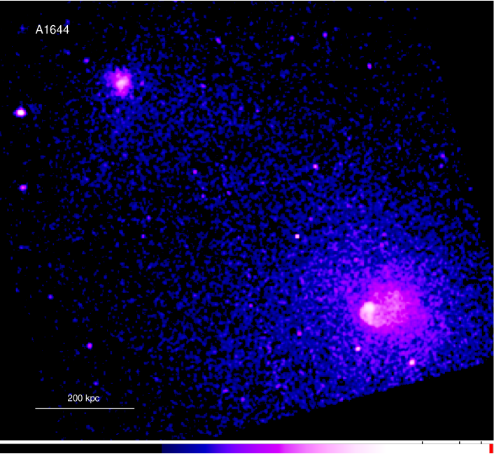
As a side note, the spiraling-in central gas should have the same direction of the angular momentum as the infalling subcluster. Thus, looking at the brightness peak in A1644 (Fig. 17), we can immediately say that the subcluster must have passed it on the eastern side. Indeed, Reiprich et al. (2004) conclude the same from their analysis of the temperature and abundance distributions obtained with XMM.

2.3.3 Origin of density discontinuity
While cold fronts may be caused by different events in the cluster, the density discontinuities in them form for the same basic reason, which is worth a clarifying aside. Simulations show that whenever a gas density peak encounters a flow of ambient gas, a contact discontinuity quickly forms. This occurs even when the initial gas distribution was perfectly smooth (no shocks, etc.), as in a merger with a pure dark matter subcluster considered above. Stripping by a shear flow is usually quoted as the cause of the discontinuity (e.g., M00; V01). Indeed, the gas pressure immediately inside the cold front in A3667 was found to be equal to the pressure of the outer gas everywhere along the front, if one models the velocity field around the spherical front and uses the Bernoulli equation (Vikhlinin & Markevitch 2002, hereafter V02; see §3.3.1 below). This suggests that the outer, less dense layers of the subcluster’s gas are quickly removed until the radius is reached where the pressure in the cold gas equals the pressure outside. It is easy to imagine how a shear flow would strip the subcluster’s gas at the sides of the front. However, at the forward tip of the front (the stagnation point), there is no shear flow for symmetry reasons, but the fronts are just as sharp.
A simple reason for the emergence of a discontinuity at the stagnation point is illustrated in Fig. 23. When an initially smooth spherical density peak starts moving w.r.t. the surrounding gas, it starts experiencing ram pressure, which creates roughly the same (area-proportional) net force for each cubic centimeter of the gas in the core (near the symmetry axis and assuming subsonic motions). Denser gas experiences smaller resulting acceleration. This produces a velocity gradient inside the core along the direction of the force. The lower-density, outer layer of the core gas is then squeezed to the sides, and the ambient gas eventually meets the dense gas for which the forward-pulling, density-proportional gravity force (as in the bullet cluster) or inertial force (as in the sloshing central gas) prevails over the area-proportional ram pressure force. The initial density peak has to be sufficiently sharp to ensure that the compressed intermediate gas does not decelerate the denser gas behind it before being squeezed to the sides, a condition which appears to be easily satisfied in real clusters. Thus, a contact discontinuity at the stagnation point forms by “squeezing out” the gas layers not in pressure equilibrium with the flow. Of course, stripping by the shear flow does occur away from the axis of symmetry of the cold front. For an illustration based on simulations, see Fig. 23 in A06.
2.3.4 Effect of sloshing on cluster mass estimates
Any motion of gas in the cluster core obviously represents a deviation from hydrostatic equilibrium and thus poses a problem for the derivation of the total masses based on this assumption (eq. 2). As we saw above (A06), in clusters that may be perfectly relaxed outside their cool cores, the central low-entropy region is easily disturbed and may not subsequently come to equilibrium for a long time. Unfortunately, “relaxed” clusters almost always have those easily disturbed cooling flow regions.
How this may affect the hydrostatic mass estimates is illustrated by the example of A1795 summarized above (Fig. 15). Using the gas profiles from the sector containing the front, the total mass within the edge radius was underestimated by a factor of 2. If one uses the radial profiles averaged over the full 360∘ azimuth, the effect is diluted; on the other hand, the edge in A1795 is relatively small. Pending a more quantitative analysis of this issue (e.g., emulating the hydrostatic mass estimates for the simulated clusters with sloshing), we can estimate roughly that masses within the cooling flow regions can be underestimated by up to a factor of 2. (The average result should always be an underestimate, since the cool gas is gravitationally bound but has a mechanical component to its total pressure, which we omit by measuring only the thermal component.) Recall that even if a cooling flow cluster does not exhibit cold fronts, statistically, it is likely to have one (or more) hidden by projection. To keep this in proper perspective, the radii of the cooling flow regions, kpc, contain only a few percent of the cluster total mass, so this systematic mass error is relevant only for a narrow range of studies, such as the exact shapes of the central dark matter cusps in clusters, or comparison of X-ray derived masses with those from strong gravitational lensing.
2.3.5 Effects of sloshing on cooling flows
XMM and Chandra observations have not found the amounts of cool gas in the centers of cooling flow clusters predicted by simple models based on the cluster X-ray brightness profiles (see Peterson & Fabian 2006 for a review). This means that that there has to be a steady energy supply to compensate for the (directly observed) radiative cooling. Several mechanisms have been proposed; the currently favored view is that AGNs, found in most cD galaxies in the centers of cooling flows, provide the heating via the interaction of AGN jets with the ICM (e.g., Voit & Donahue 2005; Fabian et al. 2005). A difficulty of this mechanism is that heating has to be steady and finely tuned (to avoid blowing up the entire cluster core), whereas AGNs have different powers in different clusters, and some clusters do not even have a presently active central AGN. In the latter clusters, other heating mechanisms may be needed for the cooling flow suppression. One of the possible alternatives is sloshing, which may have two effects. First one is obvious — M01 estimated that the mechanical energy in the sloshing gas in A1795 is around half of its thermal energy (an estimate for an analogous edge in Perseus is 10–20%, Churazov et al. 2003). As the gas sloshes, this energy is converted into heat at a steady rate.
Another effect is more interesting and possibly more significant. As seen in Fig. 21, sloshing brings hot gas from outside the cool core into the cluster center, where it comes in close contact with the cool gas that oscillates with a different period, as discussed in §2.3.2. Provided that the two phases can mix, this should result in heat inflow from the large reservoir of thermal energy in the gas outside of the cool core. A classic electron heat conduction was proposed to tap that reservoir, but was shown to be insufficient to balance the cooling (Voigt & Fabian 2004 and references therein), mainly because of the strong temperature dependence of this process. However, a “heat conduction” caused by the above mixing may be an attractive mechanism (Markevitch & Ascasibar, in preparation).
2.3.6 Effect of sloshing on central abundance gradients
Heavy elements in cooling flow clusters are concentrated toward the center (e.g., Fukazawa et al. 1994; Tamura et al. 2004; for ideas why see, e.g., Böhringer et al. 2004). Their relative abundance starts to increase just at the radii where the temperature starts to decrease (e.g., Vikhlinin et al. 2005). Cold fronts found around these gas density peaks form as a result of displacement of the central, higher-abundance gas outwards. Thus, the abundance should be discontinuous across these fronts, as long as sloshing occurs within the region with the strong gradient. Such abundance discontinuities were indeed observed, e.g., in A2204 (Sanders et al. 2005) and Perseus (Fabian et al. 2006), although Dupke & White (2003) did not see them in A496 (but their measurement uncertainties were relatively large). In general, sloshing should spread the heavy elements from the center outwards — but not too far, because, as we have seen above (§2.3.2), the low-entropy, high-abundance gas eventually flows back into the center even as a cold front continues to propagate outwards.
2.4 Zoology of cold fronts
In the sections above, we have discussed cold fronts in merging clusters and in cooling flows. Since we now know more than two clusters with cold fronts, we ought to propose a classification scheme, which will also help to summarize the above observations and simulations. First, in mergers with cold fronts that are a boundary between gases from two distinct subclusters, the front can be at the “stripping” and the “slingshot” stages. At the most intuitive “stripping” stage, ram pressure of the ambient gas pushes the cool subcluster gas back from its dark matter host; the examples are 1E 0657–56 (Figs. 1 and 38) and NGC 1404 (Fig. 6). This is likely to occur on the inbound part of the subcluster trajectory or around the time of core passage, when the ram pressure increases and reaches its maximum. A less massive subcluster may be completely stripped of gas at this stage (e.g., right panel in Fig. 10). If it does retain gas, on the outbound leg of the trajectory, the ram pressure drops rapidly (because both the ambient gas density and the velocity decrease), and the displaced gas rebounds as in a “slingshot”, overtaking the subcluster’s mass peak. An example is A168 (Fig. 11). In Fig. 12, the subcluster in the left panel and the main cluster in the right panel exhibit cold fronts at the “slingshot” stage, while the main cluster in the left panel is at the “stripping” stage.
A third variety is the “sloshing” cold fronts observed in the centers of clusters that exhibit sharp radial entropy gradients (i.e., cooling flows). Here, multiple near-concentric discontinuities divide gas parcels from different radii of the same cluster that came into contact due to sloshing (§2.3.2). Simulations show (A06) that it is set off easily by any minor merger and may last for gigayears. This is why this cold front species is very common, often with multiple fronts in the same cluster. For comparison, the core passage stage of a merger is very short (of order yr), and we should also be lucky enough to observe it from the right angle, which makes “stripping” cold fronts the rarest.
2.5 Non-merger cold fronts and other density edges
Because the central dense gas in cooling flow clusters is so easily disturbed, in principle, sloshing can also be induced by bubbles blown by the central AGNs. This possibility has not yet been addressed with detailed simulations, although some works suggest that such disturbance is possible (Quilis, Bower, & Balogh 2001). A rising bubble can also push the low-entropy gas in front of it (provided the ensuing instabilities can be suppressed), which would develop a cold front when it moves into a lower-density, lower-pressure outer region.
Edge-like features in the X-ray images of clusters and groups may have an altogether different nature. The obvious bow shocks caused by mergers will be discussed later. Edges in the cores of clusters harboring powerful AGNs may be weak shocks propagating in front of large AGN-blown bubbles, as observed, e.g., in the Hydra-A cluster (Nulsen et al. 2005). Such edges look somewhat different from the “sloshing” edges considered above, spanning a larger sector — in Hydra-A, it can be traced almost all the way around the cluster core. In addition, very subtle brightness edges or “ripples” observed in the core of the Perseus cluster have been attributed to sound waves from the central AGN explosions (Fabian et al. 2006). Because such features always have very low brightness contrast and therefore are strongly affected by line-of-sight projection, and because weak shocks have inherently low temperature contrast, it is difficult to distinguish such features from cold fronts by simply looking at their temperature profiles.
Finally, we mention a more exotic possibility of an “iron front”, as reported for the NGC 507 group (Kraft et al. 2004). An X-ray image of this cool group exhibits an edge, and the spectral analysis shows that most of the brightness difference is due to a higher abundance of heavy elements on one side of the edge (which strongly increases the emissivity for a plasma at keV). Physically, this is still a contact discontinuity similar to a cold front.
3 COLD FRONTS AS EXPERIMENTAL TOOL
The origin of cold fronts is certainly interesting, but the most useful thing about this phenomenon is that it provides a unique tool to study the cluster physics, including determining the gas bulk velocity (and sometimes acceleration, as we already saw above), the growth of hydrodynamic instabilities (or lack thereof), strength and structure of the intracluster magnetic fields, thermal conductivity, and perhaps viscosity of the ICM. We will discuss some of these possibilities below. From a technical viewpoint, what makes these studies possible is the high contrast and symmetric shape of cold fronts in the X-ray images, which enables accurate deprojection of various three-dimensional quantities near the front.
3.1 Velocities of gas flows
As we mentioned above, in broad terms, thermal pressure of the gas inside the cold front balances the sum of thermal and ram pressures of the gas outside. Both components of thermal pressure, the gas density and temperature, can be measured directly from the X-ray data, but not the velocity in the plane of the sky. The difference of thermal pressures across the front gives the ram pressure and thus the velocity of the gas cloud. This method was first applied by V01 to the cold front in A3667 (Fig. 3).
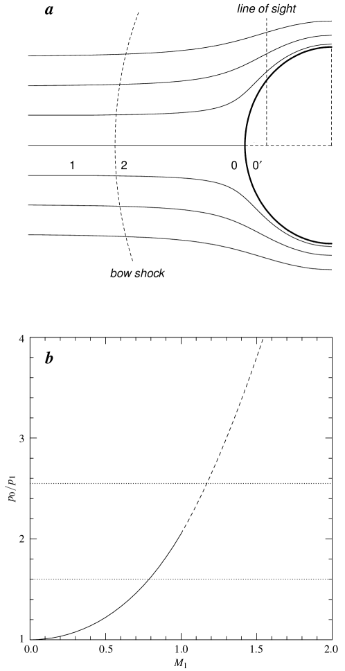
For a quantitative estimate, we must consider a more exact physical picture, schematically shown in Fig. 24 (reproduced from V01). Panel a shows a uniform flow around a stationary blunt body of dense gas. The flow forms a stagnation region at the tip of the body (zone 0), where the velocity component along the axis of symmetry goes to zero. Note that thermal pressure increases in the stagnation region as one moves closer to the front, and is continuous across the front (unlike that across a shock). The gas is compressed adiabatically, i.e., there will be a density and temperature increase in the stagnation region compared to the values in the flow (absent complications such as those discussed in §3.4.1 below). The “outer gas pressure” in the argument above is the pressure in the free-stream region of the flow (zone 1), at a sufficient distance from the front beyond the stagnation region ( of the front’s radius of curvature for a transonic flow), or ahead of the shock front if . In practice, the stagnation region is small and difficult to detect because of the line-of-sight projection, so a typical observed pressure profile derived in wide radial bins across a moving cold front would exhibit a jump.
The ratio of thermal pressures at the stagnation point, , and in the free stream, , is a function of the cloud speed (Landau & Lifshitz 1959, §114):
| (5) |
| (6) |
where is the Mach number of the cloud relative to the sound speed in the free stream region and is the adiabatic index of the gas. The subsonic equation (5) follows from Bernoulli’s equation. The supersonic equation (6) accounts for the gas entropy jump at the bow shock. Figure 24b shows these ratios as a function of .
The gas parameters at the stagnation point usually cannot be measured directly, because the stagnation region is physically small and its X-ray emission is strongly affected by projection. However, as we mentioned, thermal pressure at the stagnation point equals thermal pressure within the cloud, which is easily determined.
Because the cluster has a gradient of the gravitational potential, the gas pressure increases toward the center of a cluster in hydrostatic equilibrium, which is of course not included in eqs. (5-6). This change may not be negligible on a distance between zones 1 and 0. Because most clusters are reasonably centrally symmetric on large scales, one can usually correct the free-stream pressure for this effect with sufficient accuracy by fitting a centrally symmetric pressure model in a representative image area that excludes the front and its disturbed vicinity, and evaluating it at the radius of the front.
For the cold front in A3667, V01 obtained the ratio of the pressures (horizontal dashed lines in Fig. 24), which corresponds to , i.e. the gas cloud moves at the sound speed of the hotter gas. Evaluating the sound speed from the X-ray temperature, the cloud velocity is km s-1. In another example, Machacek et al. (2005) performed a similar analysis of the cold front at the boundary of the galaxy NGC 1404 and derived , which corresponds to the galaxy’s velocity of km s-1 relative to the ambient gas in the Fornax cluster. Mazzotta et al. (2003) obtained for a prominent cold front in 2A 0335+096, and O’Hara et al. (2004) obtained for a front in A2319, which are examples of clusters with sloshing cool cores. In A1795, the pressures at two sides of the cold front are equal, which corresponds to zero velocity (M01 and §2.3 above). There are only a few observed mergers with .
3.2 Thermal conduction and diffusion across cold fronts
Cold fronts are remarkably sharp, both in terms of the density and the temperature jumps. Ettori & Fabian (2000) first pointed out that the observed temperature jumps in A2142 require thermal conduction across cold fronts to be suppressed by a factor of order 100 compared to the collisional Spitzer or saturated values. Furthermore, V01 have found that for A3667, the gas density discontinuity at the cold front is several times narrower than the electron mean free path with respect to Coulomb collisions. Figure 25 (an update of a similar plot in V01) shows a detailed X-ray surface brightness profile across the tip of the front. The X-ray brightness increases sharply within 2–3 kpc from the front position. We can compare this width with the Coulomb mean free path of electrons (and protons, ) in the plasma on both sides of the front. The Coulomb scattering of particles traveling across the front can be characterized by four different mean free paths: that of thermal particles in the gas on each side of the front, and , and that of particles from one side of the front crossing into the gas on the other side, and . From Spitzer (1962), we have for or :
| (7) |
and for and :
| (8) |
| (9) |
where and is the error function. For the front in A3667, kpc, kpc, kpc, kpc. The upper bounds in the above intervals correspond to the expected temperature increase in the stagnation region (which is difficult to measure due to strong projection effects), and the lower bounds correspond to no increase from the observed outer temperature.
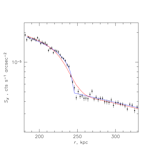
The hotter gas in the stagnation region has a low velocity relative to the cold front. Therefore, diffusion, undisturbed by the gas motions, should smear any density discontinuity by at least several mean free paths on a very short time scale. Diffusion in our case is mostly from the inside of the front to the outside, because the particle flux through the unit area is proportional to . Thus, if Coulomb diffusion is not suppressed, the front width should be at least several times . Indeed, the time for keV protons to travel 10 kpc is yr, compared to the age of the structure of at least yr, where and are the front radius and velocity. Such a smearing is ruled out by the sharp rise in the X-ray brightness at the front (Fig. 25). Fitting the observed surface brightness profile by a projected abrupt density discontinuity smeared with a Gaussian, we obtain a formal upper limit on the Gaussian of 4 kpc. One should remember that because the front is seen along the surface in projection, any deviations from the ideal spherical shape would smear the edge, and yet the observed front is sharper than the Coulomb m.f.p. This can be explained only if the diffusion coefficient is suppressed by at least a factor of 3 with respect to the Spitzer value. (This is a very conservative upper limit, simply equal to the ratio of the Spitzer m.f.p. and our upper limit on the front width; in fact, the front should spread by much more than one m.f.p. during its presumed lifetime.)
The suppression of transport processes in the intergalactic medium is most naturally explained by the presence of a magnetic field perpendicular to the density or temperature gradient. Even a very small field is sufficient for the electron and proton gyro radii to be many orders of magnitude smaller than the Coulomb m.f.p. in the ICM, so electrons and ions would move mostly along the field lines. The observation of a sharp density discontinuity in A3667 is a first direct indication that such a suppression is possible in the ICM (although this has, of course, been expected, since radio observations have provided evidence for microgauss-level magnetic fields in the ICM, see, e.g., Carilli & Taylor 2002). In many other clusters, e.g., A2142, the front width is also unresolved by Chandra, but the data quality does not allow such accurate constraints.
The suppression of diffusion and collisional thermal conduction is most effective if the magnetic field lines do not cross the front surface, that is, the two sides of the front are magnetically isolated. Below we will see that the cold front in A3667 provides another, indirect indication of just such a field configuration, with field lines mostly parallel to the front surface. We will also see why such a configuration should arise naturally in a cluster merger.
3.3 Stability of cold fronts
Cold fronts are remarkably smooth in shape, considering that they form in a violent merger environment. This property contains information on their underlying dark matter distribution, as well as conditions in the ICM, possibly including its viscosity, the prevalence of turbulence, and strength and structure of the magnetic fields. These ICM properties can significantly impact such diverse problems as the energy balance in the cluster cooling flows and estimates of the cluster total masses.
3.3.1 Rayleigh-Taylor instability and underlying mass
When a dense gas cloud moves through a more rarefied medium, ram pressure of the ambient flow slows it down. In the decelerating reference frame of the cloud, there is an inertial force directed from the dense phase to the less-dense phase, which makes the front interface of the cloud Rayleigh-Taylor unstable. As a result, the cloud quickly disintegrates, as observed in laboratory and numerical experiments, see Fig. 26. If a gas cloud is bound by gravity, it can prevent the onset of the RT instability. It is interesting to see if, for example, the cold front in A3667 is stable in this respect (V02). The drag force on the cloud is , where and are the gas density and velocity of the ambient flow, is the cloud cross-section area, and is the drag coefficient. For the particular geometry of the front in A3667 (a cylinder with a rounded head), . From the measured density inside the cloud, , we can roughly estimate the mass of the cloud as a sphere with radius , . Then the drag acceleration is:
| (10) |
For the measured quantities in A3667, cm s-2. One can also estimate the gravitational acceleration at the front surface created by the gas mass inside the cloud, which points in the opposite direction. It turns out to be times smaller, which means that gravity of the gas itself is insufficient to suppress the RT instability. Because the front is apparently stable, this means that there has to be a massive underlying dark matter subcluster, centered inside the front, that holds the gas cloud together. This is, of course, what we expect in a merger. If the total mass of the underlying dark matter halo is the usual factor of higher than the gas mass, its gravity at the front surface would be more than sufficient to compensate for the drag force, thereby removing the RT instability condition.

Pressure along the front and the underlying dark matter halo
The A3667 cold front also provides another indication of the existence of a massive dark matter halo binding the gas. Following the Bernoulli law, the pressure of the ambient flow at the surface of the front should have a maximum at the stagnation point and decline as one moves along the front surface away from the symmetry axis, as the shear velocity increases. Figure 27a (from V02) shows the measured thermal pressure just inside the surface of the front as a function of the angle from the axis of symmetry.222The data used by V02 were consistent with an isothermal gas inside the front, so the pressure in Fig. 27a was derived assuming a constant temperature (i.e., what changes in the plot is the gas density). A more recent XMM observation uncovered spatial temperature variations there (Briel et al. 2004), in particular, a cooler spot at the tip of the front. This would reduce the peak pressure somewhat; however, qualitatively and methodologically, the V02 result still holds. It behaves as expected if the front surface was in pressure equilibrium with the ambient flow. The expected ambient pressure for a flow (from a simple simulation) is also shown for comparison; it describes the measured profile very well. This indicates that the front is stationary (i.e., it is not an expanding shell, for example).
Furthermore, because the density is not constant inside the cool gas along the front, there has to be an underlying mass concentration that supports the resulting pressure gradient. Indeed, under the simplifying assumption that the gas temperature is constant, the hydrostatic equilibrium equation (2) can be written as , where is the gas density and is the gravitational potential. The declining gas pressure along the front requires a corresponding rise of the potential — Fig. 27b schematically shows the required configuration.
In V02, we presented an estimate of what kind of mass concentration is needed for the gas inside the cold front to be in hydrostatic equilibrium and exhibit such a pressure profile at the front. For a spherical halo with a King radial mass profile, the center of the halo should be located kpc under the front surface (compare this to the front radius of curvature of 250 kpc), and a total mass within kpc should be approximately . This is about 20 times higher that the gas mass in the corresponding region. Thus, the dark halo and the gas inside the cold front together look like a typical merging subcluster. The overall picture of A3667 is quite similar to the Roettiger et al. (1998) simulated merger shown in Fig. 8, and to that in the cosmological simulations by Nagai & Kravtsov (2003).
Let us now take another look at the X-ray and lensing maps for 1E 0657–56 (Figs. 1bc or 38). The ram pressure has just pushed the gas bullet out of its host dark matter halo. The halo’s gravity can no longer prevent the RT instability, and the gas bullet is expected to fall apart very quickly, although it has not happened yet (Fig. 28a). Indeed, another cluster, A520, exhibits a cool subcluster at a slightly later stage, see Fig. 28b. Similarly to 1E 0657–56, A520 is going through a supersonic merger in the plane of the sky. Its mass map also reveals a small dark matter halo located ahead of what remains of the gas subcluster (Okabe & Umetsu 2007; Clowe et al. in preparation). Apparently, A520 has already proceeded to a stage when the instabilities have broken up the cool subcluster into several pieces (Markevitch et al. in preparation).
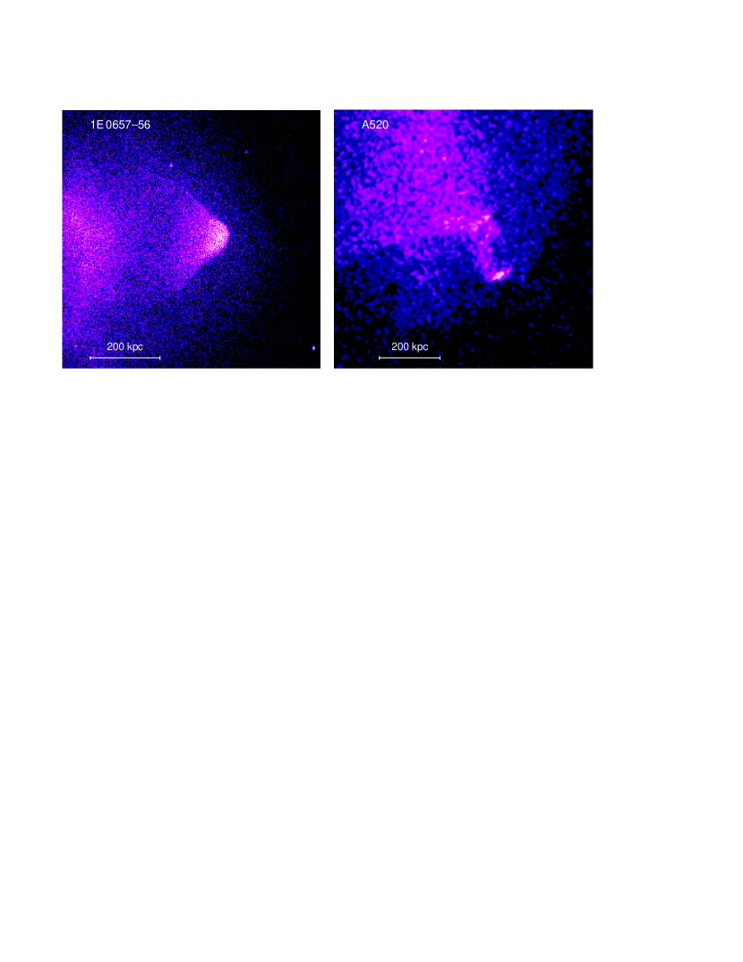
3.3.2 Kelvin-Helmholtz instability and magnetic field
Vikhlinin, Markevitch, & Murray (2001a) pointed out that the shape of the cold front in A3667 provides an independent constraint of the magnetic field at the location of the front. Their argument is that the cold front in A3667 (Fig. 3) is sharp and has a smooth shape within a certain sector () around the symmetry axis. At the same time, given the measured subcluster velocity, the front should be quickly disturbed by the Kelvin-Helmholtz (KH) instability. It would be observed in projection as smearing of the sharp edge on a width scale comparable to the wavelength of the mode that has reached the nonlinear growth stage. Thus, within that sector, the KH instability appears to be suppressed, at least for perturbations with greater than the observed upper limit on the width of the front there.
The gravity of the subcluster can in principle suppress the KH instability, just as it does the RT instability (§3.3.1). However, an estimate shows that it is far too small (V02). Assuming the density discontinuity is sharp (to which we will return below), the next most natural stabilizing mechanism is the formation of a layer of magnetic field parallel to the front. Such a layer would provide surface tension and make it difficult for any deformations of the surface to grow (Fig. 29). As we will discuss below, a layer of increased magnetic field parallel to the surface is indeed expected to emerge as a result of “magnetic draping”, i.e., stretching of the field in the ambient ICM as it flows around the cold front (e.g., Asai et al. 2005; Lyutikov 2006).
Because the shear velocity of the flow increases as one moves along the front away from the stagnation point, the surface tension of a magnetic layer at a certain angle ( in Fig. 29) may become insufficient, and the KH instability starts to grow. Thus, the extent of the undisturbed sector of a cold front may be used to derive a lower limit on the strength of the stabilizing magnetic field. Detailed calculations for a front in A3667 can be found in Vikhlinin et al. (2001a).333A minor algebraic error in that paper was pointed out by P. Mazzotta and corrected in V02, which did not change the result. Denoting the magnetic field strengths on the hot and cold sides of the front as and , the respective gas temperatures as and , the gas pressure at the front as , and the Mach number of the local shear flow as , the KH instability is suppressed when
| (11) |
For the observed temperatures and flow velocities, the observed stability of the front within the sector (where ), and taking into account the uncertainties, this gives a lower limit on the sum of magnetic pressures in the two gas phases:
| (12) |
This gives for the maximum of the two quantities and . If the apparent smearing of the front beyond the stable sector is interpreted as the onset of the KH instability, from a lower limit this becomes an estimate of the magnetic field. However, there may be other mechanisms disturbing the front at large , so it is best to consider it a lower limit.
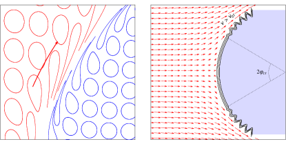
Looking at eq. (12), it is interesting to realize that even though a magnetic field is far from being “dynamically important” in the usual sense — it does not dominate the total pressure in the ICM (and thus will not significantly affect the cluster total mass estimates, for example), it can still be strong enough to qualitatively alter the evolution of cold fronts, mixing of gases, and perhaps the development of turbulence.
A more rigorous analysis of the growth of KH instability in the absence of a magnetic layer was presented by Churazov & Inogamov (2004). Their growth factor estimate for a sharp discontinuity differed from a simplified estimate in Vikhlinin et al. (2001a), but it did not change the conclusion that such a front would be unstable. More interestingly, they pointed out that the KH instability will not develop if the density discontinuity had a finite intrinsic width, for example, because of diffusion. This would completely suppress the growth of perturbations with wavelengths shorter than a certain fraction of the front radius, dependent on the smearing width. An upper limit on the width of the front from the current data (§3.2) does not rule out the Churazov & Inogamov scenario (although it comes close). We note, however, that the observed limit on the front width is already smaller by a factor of several than the collisional m.f.p., so the natural candidate to create such a stabilizing layer, collisional diffusion, does not work. A different physical process would have to widen the front within a factor of 2–3 of the current upper limit, which would require a coincidence.
While the above analyses assume a spherical shape for the front, a recent, much deeper Chandra exposure of A3667 (Fig. 3) shows that it is not exactly spherical. This would modify the flow pattern, and so the above instability suppression calculations are, of course, only qualitative.
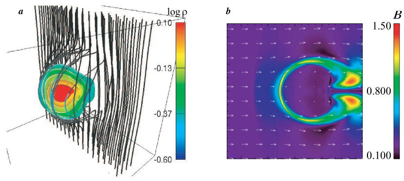
3.3.3 Origin of magnetic layer
Assuming the KH instability is indeed suppressed by the surface tension of a magnetic layer, the lower limit on the field in this layer obtained above is significantly higher than the estimates typically given for the cluster regions outside cooling flows (e.g., Carilli & Taylor 2002). This is not unexpected, because a moving cold front is a special place, where the field should align with the surface and significantly strengthen via “draping” around an obstacle, a phenomenon originally proposed by Alfvén (1957) to explain the comet tails. It is illustrated in Fig. 30 (from Asai et al. 2005). Panel (a) shows a simulation of the magnetic field lines draping around a gas cloud as the cloud moves through an ICM with a frozen-in magnetic field. These simulations used an ordered field; however, even if the field is tangled on scales less than the size of the cold front (as expected in clusters), the loops will stretch and the field at the front will consist of large two-dimensional patches (perhaps disconnected), which will have the same qualitative effect on the instabilities. Panel (b) shows the increase of the field strength at the front as a result of this shear and compression. As pointed out by Lyutikov (2006), the field can reach equipartition with the gas thermal pressure, i.e., the ratio of thermal to magnetic pressures , in a narrow layer along the surface of the front (recall that in most of the ICM, ). This effect has long been known to space physicists — it is observed by space probes at locations where the solar wind flows around the Earth magnetosphere (at magnetopause) and around the atmospheres of Mars and Venus. Similarly to the ICM, outside of such special locations, solar wind has , so the analogy is physically meaningful. Such a magnetic layer would be more than sufficient to suppress KH instabilities and completely suppress thermal conduction and diffusion across any moving cold front.
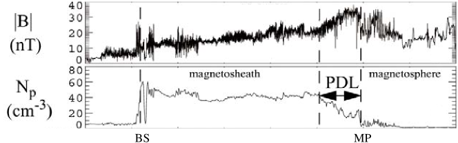
3.4 Possible future measurements using cold fronts
3.4.1 Plasma depletion layer and magnetic field
There are several interesting tests that are yet to be done using cold fronts. First, apart from stabilizing the fronts, magnetic draping mentioned in the previous section should have another directly observable effect. When magnetic pressure near the front reaches equipartition, the total (thermal plus magnetic) pressure should still satisfy the constraints imposed by the hydrodynamics of the flow. The result is that some of the plasma is squeezed out of the narrow layer near the front. The width of such a layer, , is estimated to be
| (13) |
where is the radius of the front, is the Mach number of the cloud, and and are thermal and magnetic pressures in the undisturbed gas ahead of the front (Lyutikov 2006). For cluster-sized transonic cold fronts and fields, kpc. Such “plasma depletion layers” have indeed been observed from the satellites in the corresponding locations of the solar wind (e.g., Zwan & Wolf 1976; Øieroset et al. 2004; see Fig. 31 reproduced from the latter work). If such a dip is found in the X-ray brightness profile of a cluster cold front, its width could be used for an independent estimate of the magnetic field strength in the undisturbed cluster gas.
We note that this effect will compete with the density increase in the stagnation region of the flow (§3.1). There is also a possibility of a trivial geometric “depletion” such as that seen, e.g., in the X-ray brightness profile of NGC 1404. The gas temperature inside that cold front drops well below 1 keV (Fig. 6; Machacek et al. 2005). Even though the dense gas is present, it does not emit much at keV. Combined with projection, this creates a gap along the front in the Chandra wide-band X-ray image (curious readers can extract it from the Chandra data archive). Thus, detecting a plasma depletion layer will require accurate modeling.
3.4.2 Effective viscosity of intracluster plasma
Another interesting physical quantity that may be constrained using cluster cold fronts is the effective viscosity of the ICM. For example, this unknown property of the ICM has recently attracted the attention of those studying the cluster cooling flows as a way to transfer the mechanical energy of AGN explosions into heat (e.g., Fabian et al. 2005). As we have already mentioned, the observed cold fronts appear very smooth and undisturbed by turbulence. A particularly interesting example is the bullet subcluster in 1E 0657–56 (Fig. 28), which exhibits long and straight “wisps” at its sides, where one would expect strong turbulence. There are several mechanisms that would prevent turbulence from developing; collisional viscosity is one. Even if it is suppressed (e.g., for similar reasons why thermal conduction is suppressed), there may be other kinds of viscosity specific to a magnetized plasma. Another plausible mechanism is a stabilizing magnetic layer at the cold front interface, such as the one discussed above. Such magnetic structures should not be rare; in fact, the plasma may be filled with them, because any flow in the ICM would create velocity shear and stretch the magnetic field lines around each moving gas parcel. Their net damping effect on gas mixing and turbulence may be similar to an effective viscosity. Hydrodynamic simulations that explicitly include viscosity (e.g., Sijacki & Springel 2006) would be required to derive any quantitative constraints.
For an order of magnitude estimate of what one can expect, we can look at 1E 0657–56. To prevent the development of turbulence around the gas bullet, the Reynolds number of the gas flow should be of order 10 or lower (e.g., Landau & Lifshitz 1959, §26). One can use a gasdynamic expression , where is the Mach number of the flow of gas around the bullet, is the size the bullet, and is the m.f.p. of the gas particles that determines viscosity. The condition gives in the several kpc range. Interestingly, this is comparable to the Spitzer m.f.p. in the plasma around the bullet. Thus, the effective viscosity, whatever its physical nature, may be of the order of the collisional Spitzer viscosity. Note that it may also be possible to derive upper limits on viscosity, for example, from the observed RT instability in A520 (§3.3.1), and perpahs from the presence of turbulence necessary to explain the cluster radio halos (§4.6).
4 SHOCK FRONTS AS EXPERIMENTAL TOOL
We now turn to the ICM density discontinuities of another physical nature which we always expected to find in clusters — shock fronts. There are three types of phenomena that create shocks in the ICM. As we already mentioned, in the cluster central regions, powerful AGNs often blow bubbles in the ICM, which may generate shocks within the central few hundred kpc regions (e.g., Jones et al. 2002; McNamara et al. 2005; Nulsen et al. 2005; Fabian et al. 2006; Forman et al. 2006). These shocks have . It is difficult to derive accurate temperature and density profiles for such low-contrast shocks because of large corrections for the projected emission, so they are poorly suited for our purpose of using shocks as a diagnostic tool.
At very large off-center distances (several Mpc), cosmological simulations predict that intergalactic medium (IGM) should continue to accrete onto the clusters though a system of shocks that separate the IGM from the hot, mostly virialized inner regions. The IGM is much cooler than the ICM, so these accretion (or infall) shocks should be strong, with (e.g., Miniati et al. 2000; Ryu et al. 2003). As such, they are likely to be the sites of effective cosmic ray acceleration, with consequences for the cluster energy budget and the cosmic -ray background (see, e.g., Blasi, Gabici, & Brunetti 2007 for a review). However, these shocks have never been observed in X-rays or at any other wavelengths, and may not be in the foreseeable future, because they are located in regions with very low X-ray surface brightness.
If an infalling subcluster has a deep enough gravitational potential to retain at least some of its gas when it enters the dense, X-ray bright region of the cluster into which it is falling, we may observe a spectacular merger shock, such as the one in the X-ray image of 1E 0657–56 (Fig. 1c). Such shocks can be used as tools for a number of interesting studies, which will be the subject of the rest of this review.
4.1 Cluster merger shocks
Merger shocks have been predicted in the earliest hydrodynamic simulations of cluster mergers (e.g., Schindler & Müller 1993; Roettiger, Burns, & Loken 1993; Burns 1998). They have relatively low Mach numbers, (e.g., Gabici & Blasi 2003; Ryu et al. 2003), simply because the sound speed in the gas of the main (bigger) cluster and the velocity of the infalling subcluster both reflect the same gravitational potential of the main cluster. Indeed, the central depth of the King potential is , where is the radial velocity dispersion of galaxies in this potential, which in turn is close to the average velocity of particles in the intracluster gas in hydrostatic equilibrium (e.g., Sarazin 1988). So an infalling test particle, or a small subcluster, should acquire at the center. In practice, for a merger of clusters with comparable masses (what is usually called a “major merger”), it is unlikely to observe a shock with much greater than 1. Such a merger would generate multiple successive shocks, each one significantly preheating the gas of the whole combined system, thereby reducing the Mach numbed for any subsequent shock.
Simulations also indicate that it is unlikely to find a shock front during the inbound leg of the infalling subcluster’s trajectory, because the front must climb up the steep gas density gradient of the main cluster. At the merger stage shown in top panel of Fig. 5, shock fronts may slow down and disappear while ascending the density peaks, if the peaks are high enough. At the same time, regions of the front away from the symmetry axis will continue to propagate past the density peak, and may eventually form a continuous surface behind it.
Regions of high-entropy gas in clusters have been observed with lower-resolution X-ray telescopes such as ROSAT, ASCA and XMM and interpreted as the result of shock heating (e.g., Henry & Briel 1995, 1996; Markevitch, Sarazin, & Irwin 1996b; Markevitch et al. 1999a; Belsole et al. 2003, 2004). Shock-heated regions are also routinely found by Chandra (e.g., Markevitch & Vikhlinin 2001; Markevitch et al. 2003a; Kempner & David 2004; G04). However, as of this writing, only two shock fronts, exhibiting both a sharp gas density edge and an unambiguous temperature jump, were found by Chandra, those in 1E 0657–56 (Fig. 32; M02; Markevitch 2006, hereafter M06) and A520 (Fig. 33; Markevitch et al. 2005, hereafter M05). Such finds are so rare because one has to catch a merger when the shock has not yet moved to the low-brightness outskirts, and is propagating nearly in the plane of the sky, to give us a clear view of the shock discontinuity. In addition, the shocks in A520 and 1E 0657–56 have , which provides a big enough gas density jump to enable accurate deprojection. Merger shock fronts may have been found in a couple of other clusters (e.g., in A3667, V01; A754, Krivonos et al. 2003; Henry, Finoguenov, & Briel 2004), but temperature data for them either do not exist or are uncertain. Below, we will discuss what can be learned from the fronts in 1E 0657–56 and A520.
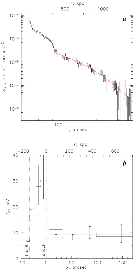
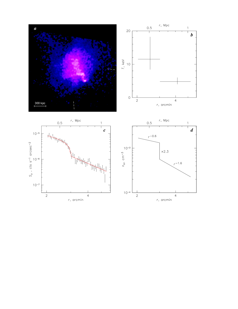
4.2 Mach number determination
Let us now look at the profiles of the X-ray brightness and projected gas temperature derived in a narrow sector crossing the bullet nose and the shock front in 1E 0657–56. They are shown in Fig. 32 (M06). From these data, we can derive a Mach number and velocity of the shock, which should also give the approximate velocity of the subcluster. In Fig. 7, we showed an approximate gas density model with two abrupt jumps, which in projection describes this brightness profile. (This fit corresponds to an early subset of the data shown in Fig. 32. Note also the different reference points for the coordinate used in Figs. 7 and 32.) The inner brightness edge in Fig. 32a is the bullet; its boundary at is a cold front, as seen from the temperature jump in panel (b) at . The edge at is the shock front, as confirmed by the temperature jump of the right sign. There is another subtle brightness edge between these main features (Fig. 32). It is unrelated to the shock, so we will exclude it when deprojecting the shock temperatures and densities.
We can determine the density discontinuity across the shock just as we did for the cold fronts, by fitting the brightness profile with a model with an abrupt spherical density jump (§2.1). The best-fit model (red line in Fig. 32a) has a density jump by a factor of 3, which includes a small correction for the observed gas temperature change across the front.
The Rankine-Hugoniot jump conditions (e.g., Landau & Lifshitz 1959, §89) relate the density jump at the shock, , and the Mach number of the shock, , where is the velocity of sound in the pre-shock gas and is the velocity of that gas w.r.t. the shock surface:
| (14) |
Using this equation, the above density jump gives a Mach number .
Note that can be derived independently using the temperature jump (using eq. 4 and the above equation), provided that the effective adiabatic index is known (i.e., no dominant relativistic particle component, significant energy leakage into particle acceleration, etc.) and that there is temperature equilibrium between electrons and ions (the latter assumption is needed only for the estimate based on the temperature jump). We will see in the next section that the observed temperature jump in 1E 0657–56 is in good agreement with the value of from the density jump. A similar analysis can be performed for the shock in A520 (Fig. 33), where a density jump by a factor of 2.3 gives , again consistent with the temperature jump (M05). For relatively weak shocks such as these, the accuracy with which we can determine from the X-ray derived density discontinuity is better than what we can do from the temperatures. However, as increases, the density jump asymptotically goes to a finite value ( for ), while the temperature jump continues to grow, so the situation reverses.
Sound speed in the pre-shock gas can be determined from its observed temperature. The above Mach numbers then give the shock velocities of 4700 km s-1 and 2300 km s-1 for 1E 0657–56 and A520, respectively. From the continuity condition, the respective velocities of the post-shock gas w.r.t. the shock surface are times lower, 1600 km s-1 and 1000 km s-1. For 1E 0657–56, the distance between the centers of merging subclusters is 720 kpc (see the weak lensing map in Fig. 38). Assuming that the bullet subcluster’s velocity is close to the shock velocity (although it can be lower, Springel & Farrar 2007; Milosavljevic et al. 2007), the two subclusters have passed through each other just 0.15 Gyr ago.
4.3 Front width
The X-ray brightness profile in Fig. 32 does not exclude a shock front of a finite width; in fact, it marginally prefers a density jump widened by a Gaussian with (35 kpc). Curiously, this is of the order of the collisional m.f.p. in the gas around the shock — but it may simply be a coincidence, since, e.g., any deformations of the front shape seen in projection would smear the edge. The best-fit amplitude of the jump that was used above to derive the Mach numbers does not depend noticeably on this width.
In this regard, it is interesting to look at simulations by Heinz & Churazov (2005), who studied propagation of a shock in an ICM filled with bubbles of relativistic plasma. Such a mixture in pressure equilibrium may form as a result of AGN activity over the cluster lifetime; cluster radio relics may be examples of such regions containing fossil relativistic plasma (e.g., Enßlin & Gopal-Krishna 2001). Because the sound speed inside such a bubble is very high, a shock front surface will be deformed on a linear scale of these bubbles. Heinz & Churazov proposed such smearing as an explanation for the lack of visible strong AGN jet-driven shocks in the cluster centers. The fact that the fronts in 1E 0657–56 and A520 can be seen at all in the X-ray images indicates that, at least in these clusters, the bulk of the ICM is not filled with fossil bubbles greater than several tens of kpc in size. On the other hand, there is an example of A665, in which the overall X-ray morphology and the temperature map suggest that there should be a shock front, and there is a gas density excess, but no density discontinuity is seen (Markevitch & Vikhlinin 2001; G04). It might be that an observable sharp discontinuity did not form there because the shock has to propagate in such a mixture.
4.4 Mach cone and reverse shock?
Before proceeding to some of the interesting shock-based measurements, we would like to address two questions that people familiar with shocks in other astrophysical contexts frequently have: the Mach cone444The Mach cone discussion here differs from the version published in Physics Reports — it is updated with results from simulations by Springel & Farrar (2007). and the reverse shock.
A small body moving supersonically creates a Mach cone with an opening angle . For , the shock in 1E 0657–56 should have an asymptotic angle of 20∘ from the symmetry axis. However, the image (Fig. 1c) shows a more widely open “Mach cone”. A possible reason is easy to understand if we consider that the bullet is not a solid body, but a gas cloud whose outer, less dense gas is being continuously stripped by the flow of the shocked gas. The tip of the bullet is becoming smaller with time, as shown schematically in Fig. 23 (see §2.3.3). The off-axis parts of the shock front that we see at present are not driven by the bullet that we see at present, but by a bigger bullet that has existed just a short while ago. Thus, the shape of the front (at least of its bright region which we can follow in the image) does not correspond to a Mach cone, but rather reflects the change of the bullet size and velocity with time. Another significant effect is the inflow of the pre-shock gas caused by the gravity of the subcluster (Springel & Farrar 2007). This inflow is faster at the nose of the shock (which currently coincides with the subcluster’s mass peak, see Figs. 1bc), which flattens the front shape.
We can test this by deriving an X-ray brightness profile across an off-axis stretch of the shock front, e.g., in a narrow sector pointing 30∘ clockwise from the bullet velocity direction. For a stationary oblique shock with such an angle to the uniform upstream flow, the density jump should be reduced from 3.0 at the nose to 2.8 (e.g., Landau & Lifshitz 1959, §92). However, the observed jump is a factor of 2.1, which corresponds to a smaller . This is consistent with a higher inflow velocity of the pre-shock gas at the nose of the shock.
In addition, the main cluster’s radially declining density profile, in which the shock propagates, and deceleration of the bullet by gravity and ram pressure should also affect the shape of the front (M02).
Those working with supernova remnants (SNR) may also ask where is the reverse shock in 1E 0657–56 — a front that propagates inwards from the outer surface of an SNR. If we look at the scheme in Fig. 5, it is clear that the reverse shock for shock 1 is shock 2, and vice versa. The current stage of the merger in 1E 0657–56 corresponds to the bottom panel in Fig. 5. By this time, the reverse shock has attempted to climb the sharp density peak of the bullet subcluster, but failed to penetrate inside the radius where we now have a cold front. As mentioned in §4.1, the outer regions of that shock must have moved past the bullet and away from the picture; from the symmetry, it should be somewhere on the opposite side from the cluster center.
4.5 Test of electron-ion equilibrium
The post-shock temperature that enters the Rankine-Hugoniot jump conditions is the temperature that all plasma particle species acquire when they reach equilibrium after the shock passage. In a collisional plasma, protons, whose thermal velocity is lower than the shock velocity, are heated dissipatively at the shock layer that has a width of order the collisional m.f.p. The faster-moving electrons do not feel the shock (for ) and are compressed adiabatically. Subsequently, electrons and protons equilibrate via Coulomb collisions on a timescale (e.g., Zeldovich & Raizer 1967)
| (15) |
For a shock in a magnetized plasma such as the ICM, the final post-shock temperature should be the same (provided that the kinetic energy does not leak into cosmic rays, etc.), but the shock structure can be very different. Indeed, studies of solar wind shocks in-situ showed that the electron and proton temperature jump occurs on a linear scale of order several proton gyroradii, many orders of magnitude smaller than their collisional m.f.p. (Montgomery, Asbridge, & Bame 1970 and later works), which is why these shocks are called collisionless. Therefore, it would not be surprising to find a different rate of electron heating at the shock, and a shorter electron-proton equilibration timescale. (To find a longer timescale would be surprising, because Coulomb collisions do occur even in the “collisionless” plasma.)
The bow shock in 1E 0657–56 offers a unique experimental setup to determine how long it takes for post-shock electrons to come to thermal equilibrium with protons in a magnetized plasma (M06). Given the likely turbulent widening of the heavy ion emission lines (and, of course, for lack of the required energy resolution at present), we cannot directly measure in X-rays, only . However, we can use the accurately measured gas density jump at the front (§4.2) and the pre-shock electron temperature to predict the post-shock adiabatic and instant-equilibration electron temperatures, using the adiabatic and the Rankine-Hugoniot jump conditions, respectively, and compare them with the data. Furthermore, we also know the downstream velocity of the shocked gas flowing away from the shock (1600 km s-1, §4.2). This flow effectively spreads out the time dependence of the electron temperature along the spatial coordinate in the plane of the sky. The Mach number of the 1E 0657–56 shock is conveniently high, such that the adiabatic and shock electron temperatures are sufficiently different (for , they become close and difficult to distinguish, given the temperature uncertainties). It is also not a strong shock, for which the density jump would just be a factor of 4 and would not let us directly determine . Furthermore, the distance traveled by the post-shock gas during the time given by eq. (15), kpc , is well-resolved by Chandra.
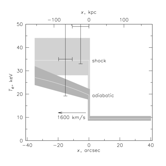
As we already mentioned, there is a subtle secondary brightness edge between the bullet and the shock, behind which the temperature decreases (Fig. 32). It is most likely caused by residual cool gas from the subcluster in one form or another, and is unrelated to the shock. Therefore, we can use only the temperature profile between the shock and this edge, where we have two bins. Using the gas density profile in front of the shock, we can subtract the contributions of the cooler pre-shock gas projected onto these post-shock bins, assuming spherical symmetry in this small segment of the cluster. The shock brightness contrast is high, which makes this subtraction sufficiently accurate. In Fig. 34, the deprojected temperatures are overlaid on the two models: instant equilibration and adiabatic compression with subsequent equilibration on a timescale given by eq. (15). (The plot assumes a constant post-shock gas velocity, which of course is not correct, but we are only interested in the immediate shock vicinity.) The deprojected post-shock gas temperatures are so high compared with the Chandra energy band that only their lower limits are meaningful. The temperatures are consistent with instant heating; equilibration on the collisional timescale is excluded, although with a relatively low 95% confidence. The equilibration timescale should be at least 5 times shorter than .
A few sanity checks have been performed in M06. In particular, the possibility of a non-thermal contamination of the spectra was considered. 1E 0657–56 has a radio halo (Fig. 1d; Liang et al. 2000), which has an edge right at the shock front (M02; see below). Therefore, there may be an IC contribution from relativistic electrons accelerated at the shock. However, in the Chandra energy band, the power-law spectrum of such emission for any would be softer than thermal (which for these temperatures has a flat effective photon index of ), so it cannot bias our temperature measurements high. It is unfortunate that a cluster with such a perfect geometric setup and is so hot that Chandra can barely measure the post-shock temperatures; however, there are not many of them to choose from. The available A520 data do not have the accuracy for such a measurement.
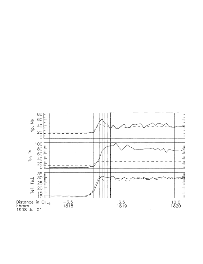
4.5.1 Comparison with other astrophysical plasmas
To our knowledge, the above result is the first direct indication for any astrophysical plasma that after a shock, electrons reach the equilibrium temperature on a timescale shorter than collisional. However, it cannot distinguish between two interesting possibilities: electrons being heated to the “correct” temperature right at the shock, or electrons and protons equilibrating soon after via a mechanism unrelated to the shock. This is where the solar wind and supernova remnants (SNR) provide complementary evidence.
A large amount of data has been gathered by space probes for the heliospheric shocks, especially for the Earth’s bow shock (for recent reviews see, e.g., Russell 2005 and references therein). Many of these shocks have high Alfvén Mach numbers , moderate sonic Mach numbers, and a ratio of pre-shock thermal to magnetic pressure , which should make them qualitatively similar to merger shocks in clusters (although and in clusters are typically much higher; e.g., upstream of the 1E 0657–56 shock, and , so the similarity is not guaranteed). In most observed heliospheric shocks, and in all the stronger ones, electrons were heated much less than protons, barely above the adiabatic compression temperature (e.g., Schwartz et al. 1988). Figure 35 gives a typical example of a shock crossing by the Wind satellite (Hull et al. 2001). Both and quickly reach their respective asymptotic values, which are . These in-situ measurements cannot tell us what happens after that on timescales comparable to (which corresponds to a linear scale of several A.U.), but they do show that equilibration at least does not occur on scales .
Another site of actively studied shocks is SNRs. The typical in SNR plasmas is of the same order of that in clusters, much higher than that in the solar wind. Outer shocks in SNRs are typically very strong and may be modified by cosmic ray acceleration (see, e.g., Vink 2004 for a review). Nevertheless, these very different shocks also exhibit in most cases (e.g., Rakowski 2005; Raymond & Korreck 2005), although with considerable uncertainty due to the difficulty of estimating the velocity and for a strong shock. (One cannot use the density jump as we did, as it is at its asymptotic value; on the other hand, in some Galactic SNRs, the shock velocity can be directly measured using high-resolution X-ray images taken several years apart, which, of course, is impossible for clusters.) The typical timescale for an SNR plasma is of order yr, which in many cases is comparable to the SNR’s age. Furthermore, the region for which the temperatures are derived is usually close to the shock, so the timescales sampled by the temperature measurements in the SNR plasma are usually . Thus, similarly to the solar wind results, the SNR data indicate that collisionless shocks with a wide range of parameters produce , but, to our knowledge, do not constrain the timescale of the subsequent equilibration.
The solar wind and SNR results on one hand, and our 1E 0657–56 measurement on the other, appear to leave only one of the two possibilities mentioned above, namely, that shocks produce unequal electron and ion temperatures, which quickly equalize outside the shock layer. Proposing an equilibration mechanism that works faster than Coulomb collisions in plasma is beyond the scope of this review (and our expertise).
4.6 Shocks and cluster cosmic ray population
Cluster mergers convert kinetic energy of the gas in colliding subclusters into thermal energy by driving shocks and turbulence. A fraction of this energy may be diverted into nonthermal phenomena, such as magnetic field amplification and the acceleration of ultrarelativistic particles. Such particles manifest themselves via synchrotron radio halos (recently reviewed by, e.g., Feretti 2002, 2004; Kempner et al. 2004) and IC hard X-ray emission (e.g., Fusco-Femiano et al. 2005; Rephaeli & Gruber 2002). This energy fraction may be significant and depends on the exact mechanism of the production of halo-emitting electrons, which is not yet understood. However, a consensus emerges that the underlying cause and energy source should indeed be the subcluster mergers (e.g., Feretti 2002; Buote 2001; G04).
The radio halo generating electrons are relatively short-lived ( yr) due to IC and synchrotron energy losses (e.g., Sarazin 1999). This is much shorter than the diffusion time across a cluster-sized halo, so a mechanism is required by which these electrons are locally and simultaneously (re)accelerated over the halo volume. Several possibilities were proposed, including radio galaxies, so-called “secondary electron” production by interactions of the long-lived cosmic ray protons with the ICM protons, and “primary electron” mechanisms, in which electrons are accelerated directly by merger-driven turbulence or shocks (see, e.g., Brunetti 2003 for a review).
Shock fronts provide a unique experimental tool in this area. They are those rare locations in clusters where we can determine gas velocities in the sky plane and the gas compression ratio (§4.2). They also create high-contrast features in the cluster X-ray images and, as we will see, in the radio images. Simply by comparing the X-ray and radio images of clusters with shock fronts, one may be able to determine the contribution of shocks to the halo production.
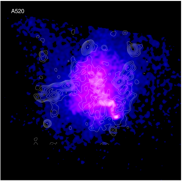
Both clusters with known shock fronts, 1E 0657–56 and A520, have prominent radio halos (Liang et al. 2000; Govoni et al. 2001). Their radio brightness contours are overlaid on the X-ray images in Figs. 1d and 36. One immediately notices a striking coincidence of the SW edge of the radio halo in A520 with the shock front (M05). A similar extension of the radio halo edge to the bow shock is seen in the less well-resolved halo in 1E 0657–56 (M02; G04). In another merging cluster, A665, a “leading” edge of the radio halo also corresponds to a region of hot gas that’s probably behind a bow shock (Markevitch & Vikhlinin 2001; G04), although the X-ray image of A665 does not show a gas density edge at the putative shock (§4.3). The cold front cluster A3667 exhibits two radio relics at the opposite sides of the cluster (Röttgering et al. 1997), along the merger axis suggested by the cold front. They are often mentioned as evidence of bow shocks at those locations; however, they are located too far in the cluster periphery, where X-ray imaging is not currently feasible.
The overall structure of the radio halo in A520 suggests two distinct components, a mushroom with a stem and a cap, where the main stem component goes across the cluster and the cap ends at the bow shock. The main halo component is located in the region of the cluster where one expects relatively strong turbulence (G04), but about which we cannot say much observationally at present. However, the part of the halo that coincides with the shock front can already be used for interesting tests. Below we discuss two main possibilities for its origin, how to distinguish between them, and propose some future tests that can be done using this shock (M05).
4.6.1 Shock acceleration
One explanation for the radio edge is acceleration of electrons to ultrarelativistic energies by the shock. The shock with a density jump should generate electrons with a Lorentz factor and energy spectrum with
| (16) |
via first-order Fermi acceleration (see, e.g., Blandford & Eichler 1987 for a review). For the A520 shock with , . The synchrotron emission should have a spectrum with right behind the shock front. However, these electrons are short-lived because of IC and synchrotron energy losses (e.g., Rybicki & Lightman 1979), and their spectrum will quickly steepen. The respective electron lifetimes, and , are
| (17) |
and
| (18) |
(e.g., Sarazin 1999). IC losses dominate for ; other losses are negligible for our range of energies and fields. For a power-law electron spectrum with (expected for shocks with ), the contribution of different at a given synchrotron frequency has a peak at
| (19) |
Assuming , the lifetime for electrons with that emit at our radio image frequency of 1.4 GHz in A520 is yr. Thus, given the 1000 km s-1 velocity of the downstream flow (§4.2) that carries these electrons away from the shock, the width of the synchrotron-emitting region should only be about 100 kpc, beyond which the electrons cool out of the 1.4 GHz band. This scale is an order of magnitude smaller than the size of the halo, so the whole halo cannot be produced by particles accelerated at this shock. A similar conclusion was reached for the front in 1E 0657–56 by Siemieniec-Oziebło (2004), and this is expected for merger shocks in general (e.g., Brunetti 2003). However, the cap-like part of the radio halo appears to have just the right width, kpc (considering the finite angular resolution). Thus, with the available data, this region is not inconsistent with shock acceleration. While the relativistic electrons in this structure cool down soon after the shock passage, some may later be picked up and re-accelerated as they reach the turbulent region behind the subcluster core, where the stem-like halo component forms.
Because the bow shock is spatially separated from the turbulent area further downstream (except for the region around the small dense core fragments) and there is no reason to expect significant turbulence and additional acceleration in that intermediate region, the cap-like structure is likely to exhibit a measurable spectral difference from the main halo. Within the 100 kpc-wide strip along the shock, the spectrum should quickly steepen starting from . If the region is unresolved, the resulting mixture would have a volume-averaged slope (Ginzburg & Syrovatskii 1964) which is significantly steeper than observed on average in most halos (e.g., Feretti 2004), the bulk of which is probably continuously powered by turbulence. Interestingly, Feretti et al. (2004) found that the presumed post-shock region in A665 indeed exhibits the steepest radio spectrum in the spectral index map of the cluster, which is consistent with the above two-component cap + stem picture.
4.6.2 Compression of fossil electrons
The efficiency with which collisionless shocks can accelerate relativistic particles is unknown, and may be insufficient to generate the observed radio brightness. The radio edges in A520 and 1E 0657–56 offer an interesting prospect for constraining it. If the acceleration efficiency is low, the observed radio edge may alternatively be explained by an increase in the magnetic field strength and the energy density of the pre-existing relativistic electrons, simply due to the gas compression at the shock. Such pre-existing electrons with energies below those required to emit at our radio frequencies (eq. 19) may accumulate from past mergers (e.g., Sarazin 1999). In this model, the pre-existing electrons must produce low-brightness diffuse radio emission in front of the bow shock, whose intensity and spectrum may be predicted from the shock compression factor and the post-shock radio spectrum.
M05 made such a prediction under the assumption that, as the plasma crosses the shock surface, each volume element, with its frozen-in tangled magnetic field, is compressed isotropically. Indeed, observations at the Earth’s bow shock show that a shock passage strengthens the field whether it is parallel or perpendicular to the shock (e.g., Wilkinson 2003), so this assumption is adequate. The average field strength then increases by a factor
| (20) |
This increase would cause the particles to spin up as (the adiabatic invariant). In addition, the number density of relativistic electrons increases by another factor of due to the compression. As a result, for a power-law fossil electron spectrum of the form , the synchrotron brightness at a given radio frequency should exhibit a jump at the shock
| (21) |
The power-law slope of the spectrum is preserved. Thus, for the A520 shock with , if the radio edge is due to the compression only, there must be a pre-shock radio emission with the same spectrum as post-shock, but fainter by a factor of for , respectively. (In practice, can be determined from the post-shock radio spectrum; this measurement is currently feasible but has not yet been made.) Of course, projection of a spheroidal shape of the shock should be taken into account, as is done for deriving the amplitude of the X-ray brightness jump.
Although the low surface brightness within the radio halos is already near the limit of detectability, an improvement of sensitivity by an order of magnitude required to look for emission from pre-shock fossil electrons is not completely out of reach. If future sensitive measurements do not detect such a pre-shock emission at the level predicted for simple compression, it would mean that the shock generates relativistic electrons and/or a magnetic field, as opposed to simply compressing them. Observations of solar wind shocks of a similar strength and as in cluster plasma, as well as lower- shocks, seem to be consistent with a simple compression of the field (e.g., Russell & Greenstadt 1979; Hull et al. 2001), so significant magnetic field generation is unlikely. Thus, such a non-detection would provide a lower limit on the shock’s particle acceleration efficiency, a quantity that is interesting for a wide range of astrophysical problems.
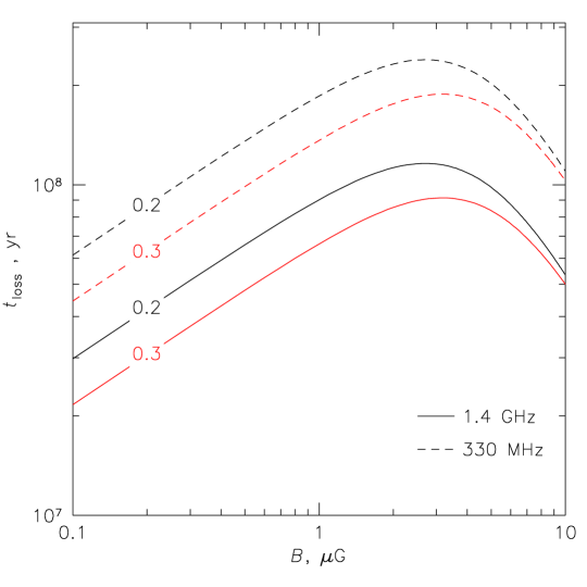
4.6.3 Yet another method to measure intracluster magnetic field
The strength of the magnetic field in the ICM is an important quantity, but its measurements are still very limited in accuracy and often restricted to certain non-representative locations in clusters (e.g., Carilli & Taylor 2002). The shock-related edge of the radio halo in A520, and perhaps a similar region in 1E 0657–56, may allow an independent estimate of the magnetic field strengths behind the shock, regardless of the exact origin of the relativistic electrons. As discussed above, IC and synchrotron cooling cause the electron spectrum to steepen and the electrons to drop out of the radio image on timescales of order yr. This timescale depends on the field strength as shown in Fig. 37, which combines eqs. (17–19). It gives the lifetime of the electrons that contribute the most emission at a given frequency, for an electron energy spectrum with the slope and an interesting range of . Assuming that the bow shock causes a momentary increase in electron energy and , and that diffusion of the relativistic particles is negligible (see M05 for a discussion), the flow of the post-shock gas (that carries the relativistic electrons with it) will spread the time evolution of the electron spectrum along the spatial coordinate — something we have already used for another test in §4.5. Thus, the width of the cap-like region of the halo can give us the magnetic field strength. Of course, the magnetic field behind the shock will be amplified from its pre-shock value as discussed in §4.6.2. This method can distinguish among the values in the currently controversial range of , although, as seen from Fig. 37, it cannot give a unique value of , because is not a monotonic function of . In practice, such a measurement will need to be done at more than one frequency, in order to determine the spectrum of the electrons and to verify that they cool as predicted at different frequencies, that is, no acceleration occurs after the shock has passed. The available single-frequency radio data (Fig. 36; Govoni et al. 2001) do not have the needed signal to noise ratio or angular resolution, but are not inconsistent with G.
4.7 Constraints on the nature of dark matter
We finally mention two interesting results that rely on the determination of the velocity and the direction of motion of the subcluster in 1E 0657–56 based on its shock front. The fact that we observe a cold front or a shock front tells that the subcluster responsible for the feature moves very nearly in the plane of the sky, because otherwise, the sharp gas density jump would be smeared by projection. From the shapes of either feature, usually the direction of motion in the sky plane is also clear, as seen in the images of A3667 (Fig. 3), NGC 1404 (Fig. 6), and 1E 0657–56 (Fig. 1c). For the latter cluster, the shock and the cold front (the bullet) in the X-ray image strongly suggest that the X-ray gas distribution has axial symmetry, at least in its western half containing the shock and the bullet. This allows a reasonably accurate estimate of the gas mass in that region. As expected from observations of other clusters, invariably showing that gas is the dominant baryonic mass component, the gas mass of the bullet is several times higher than the stellar mass in galaxies in a comparable aperture centered on the brightest galaxy of that subcluster. At the same time, comparison of the gravitational lensing mass map and the X-ray image (Fig. 38; Clowe et al. 2006; see also Bradač et al. 2006) shows that the subcluster’s total mass peak is offset from the baryonic mass peak (the X-ray bullet). The same is true for the bigger eastern subcluster. Clowe et al. (2004, 2006) interpret this as the first direct evidence for the existence of dark matter, as opposed to alternative theories that avoid the notion of dark matter by, e.g., modifying the gravitational force law on cluster scales (e.g., MOND: Milgrom 1983; Brownstein & Moffat 2006). If cluster had contained only visible matter (i.e., mostly the X-ray emitting gas), regardless of the form of the gravity law, the gravitational lensing would have to show a mass peak coincident with the gas bullet (see Clowe et al. 2006 for a more detailed discussion, and Angus et al. 2007 for a MOND response admitting the need for dark matter).
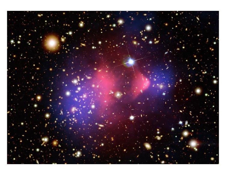
Furthermore, the current orientation of the shock and the bullet let us reconstruct the trajectory of the merging subclusters back in time at least to the core passage. It is clear that the small halo has passed near the center of the bigger halo. The shock front also gives an estimate of the current velocity of the subcluster (§4.2). Combined with the mass measurements from lensing and the distribution of the member galaxies from the optical images, this can be used to derive a limit on the self-interaction cross-section of the dark matter particles. Although the common wisdom is that dark matter is collisionless, a nonzero cross-section was proposed as a solution for several observational problems (Spergel & Steinhardt 2000). 1E 0657–56 offers an interesting opportunity to test this hypothesis in a relatively robust and model-independent way (Markevitch et al. 2004). If the dark matter particles experienced scattering by elastic collisions, it would have several observable consequences. At large cross-sections, the dark matter would behave as a fluid — just like the intracluster gas — and there would be no offset between the gas peak and the dark matter peak. This extreme is excluded simply by comparing the X-ray and mass images (Fig. 38). Smaller values would lead to subtler effects, such as an anomalously low mass-to-light ratio for the subcluster caused by loss of dark matter particles by the subcluster, and a lag of the subcluster mass peak from the centroid of the collisionless galaxy distribution. The absence of these effects gives a conservative upper limit on the cross-section of cmg-1, where is the (unknown) mass of the dark matter particle (Randall et al. 2007). This excludes almost the entire range of values (0.5–5 cmg-1) required to solve the problems for which the self-interacting dark matter has been invoked.
5 SUMMARY
Recent observations of sharp gas density edges in galaxy clusters provided us with novel ways to study the cluster mergers, and even to perform remote sensing of some otherwise inaccessible physical properties of the intracluster plasma. Classic bow shocks have been observed in two clusters undergoing violent mergers at the right stage and with the right orientation for us to see the front discontinuities unobstructed. They have been used to determine the velocities and trajectories of the infalling subclusters.
The velocity and the unique geometry of the subcluster in 1E 0657–56, whose gas is clearly stripped from its dark matter by ram pressure, were combined with the gravitational lensing and optical data to place an upper limit on the dark matter’s self-interaction cross-section, and to directly demonstrate the dark matter existence.
A jump of the electron temperature at the shock in 1E 0657–56 provides evidence that electron-ion equilibration in the ICM occurs on a timescale shorter than the collisional timescale. To our knowledge, this is the first such test in any astrophysical plasma. Combined with finding based on the shocks in solar wind and SNRs that electrons are not heated to equilibrium temperature immediately in the shock, the 1E 0657–56 result indicates the presence of a fast electron-ion equilibration mechanism unrelated to shocks (although the uncertainty of the 1E 0657–56 result is quite large).
The shock front in A520 coincides with a distinct edge-like feature in the radio halo observed in this cluster. This indicates that ultrarelativistic electrons responsible for this part of the radio halo emission are either accelerated by this weak shock, or that there is a pre-existing relativistic population that is being compressed by the shock. More sensitive radio observations will be able to distinguish among these interesting possibilities and constrain the efficiency of electron acceleration by shocks. The A520 shock also provides a setup for a measurement of the strength of the magnetic field in this cluster by determining the cooling time of the relativistic electrons.
In addition to observing shock fronts, Chandra has discovered a new kind of transient features in the intracluster gas, named “cold fronts.” These sharp density edges are contact discontinuities between gas phases with different specific entropies in approximate pressure equilibrium. They form as a result of bulk motion of a dense gas cloud through the hotter ICM. In merging clusters, these clouds are the surviving remnants of the cores of the infalling subclusters. In cooling flow clusters, such edges are produced by displacement and subsequent sloshing of the low-entropy central gas. Cold fronts are much more common than shock fronts. Just as shock fronts, they can be used to determine the velocity and the direction of motion of the gas flow.
Cold fronts are remarkably sharp and stable. The observed temperature jumps across cold fronts require thermal conduction across the front to be severely suppressed. Furthermore, the density jump in the best-observed front in A3667 is narrower than the collisional mean free path in the plasma. These observations demonstrate that transport processes in the ICM can be easily suppressed. The KH stability of the front in A3667 also suggests the presence of a layer of the compressed magnetic field oriented along the front surface, such as the one expected to form as a result of magnetic draping. Such a layer is exactly what is needed to completely suppress thermal conduction and diffusion across the front surface. In addition, Rayleigh-Taylor stability of the front in A3667 reveals the presence of an underlying massive dark matter subcluster.
This area of cluster research is relatively new (although much of the underlying hydrodynamics is textbook). It is not yet completely clear what these findings mean for the more general questions of how the energy is dissipated in a cluster merger, how much of it goes into relativistic particles and magnetic fields, how prevalent and long-lived is turbulence, how effective is mixing of the various gas phases, what is the effect of the central gas sloshing and turbulence on cooling flows and on the hydrostatic mass estimates, how representative of the hydrostatic temperatures are the average temperatures derived from the X-ray data, etc. Our goal for this mostly observational review was to encourage detailed theoretical and numerical studies of these interesting phenomena that can be used as novel diagnostic tools in clusters.
References
- (1)
- jnk (1999) Abell, G. O. 1958, ApJ Suppl., 3, 211
- jnk (1999) Acreman, D. M., Stevens, I. R., Ponman, T. J., Sakelliou, I., 2003, MNRAS, 341, 1333
- jnk (1999) Alfvén, H. 1957, Tellus, 9, 92
- jnk (1999) Allen, S. W., Schmidt, R. W., & Fabian, A. C. 2001, MNRAS, 328, L37
- jnk (1999) Allen, S. W., Schmidt, R. W., Ebeling, H., Fabian, A. C., & VanSpeybroeck, L. 2004, MNRAS, 353, 457
- jnk (1999) Allen, S. W., Schmidt, R. W., & Fabian, A. C. 2002, MNRAS, 334, L11
- jnk (1999) Angus, G. W., Shan, H. Y., Zhao, H. S., Famaey, B., 2007. ApJ, 654, L13
- jnk (1999) Arnaud, M., et al. 2001, A&A, 365, L67
- jnk (1999) Asai, N., Fukuda, N., & Matsumoto, R. 2005, Adv. Space Research, 36, 636 (astro-ph/0504227)
- jnk (1999) Ascasibar, Y., & Markevitch, M. 2006, ApJ, 650, 102 (A06)
- jnk (1999) Bahcall, J. N., & Sarazin, C. L. 1977, ApJ, 213, L99
- jnk (1999) Bartelmann, M., & Schneider, P. 2001, Phys. Reports, 340, 291
- jnk (1999) Belsole, E., Pratt, G. W., Sauvageot, J.-L., & Bourdin, H. 2003, A&A, 430, 385
- jnk (1999) Belsole, E., Pratt, G. W., Sauvageot, J.-L., & Bourdin, H. 2004, A&A, 415, 821
- jnk (1999) Bialek, J. J., Evrard, A. E., & Mohr, J. J. 2002, ApJ, 578, L9
- jnk (1999) Blandford, R. & Eichler, D. 1987, Phys. Reports, 154, 1
- jnk (1999) Blasi, P., Gabici, S., & Brunetti, G. 2007, Int. J. Mod. Phys. A, 22, 681 (astro-ph/0701545)
- jnk (1999) Böhringer, H., Matsushita, K., Churazov, E., Finoguenov, A., & Ikebe, Y. 2004, A&A, 416, L21
- jnk (1999) Bradač, M., et al. 2006, ApJ, in press
- jnk (1999) Briel, U. G., Finoguenov, A., & Henry, J. P. 2004, A&A, 426, 1
- jnk (1999) Briel, U. G., Henry, J. P., & Boehringer, H. 1992, A&A, 259, L31
- jnk (1999) Brownstein, J. R., & Moffat, J. W. 2006, MNRAS, 367, 527
- jnk (1999) Brunetti G., 2003, Proc. “Matter and Energy in Clusters of Galaxies”, Taiwan, ASP Conf. Series, eds. S. Bowyer & C.-Y. Hwang, 301, 349 (astro-ph/0208074)
- jnk (1999) Buote, D. A., 2001, ApJ, 553, L15
- jnk (1999) Buote, D. A. & Tsai, J. C. 1996, ApJ, 458, 27
- jnk (1999) Burns, J. O. 1998, Science, 280, 400
- jnk (1999) Carilli, C. L. & Taylor, G. B. 2002, ARA&A, 40, 319
- jnk (1999) Cavaliere, A., & Fusco-Femiano, R. 1976, A&A, 49, 137
- jnk (1999) Chandran, B. D. G., & Cowley, S. C. 1998, Phys. Rev. Lett., 80, 3077
- jnk (1999) Churazov, E., Forman, W., Jones, C., and Böhringer, H. 2003, ApJ, 590, 225
- jnk (1999) Churazov, E., & Inogamov, N. 2004, MNRAS, 350, L52
- jnk (1999) Clarke, T. E., Blanton, E. L., & Sarazin, C. L. 2004, ApJ, 616, 178
- jnk (1999) Clowe, D., Bradač, M., Gonzalez, A. H., Markevitch, M., Randall, S. W., Jones, C., & Zaritsky, D. 2006, ApJ, 648, L109
- jnk (1999) Clowe, D., Gonzalez, A. H., & Markevitch, M. 2004, ApJ, 604, 596
- jnk (1999) De Grandi, S., & Molendi, S. 2002, ApJ, 567, 163
- jnk (1999) Dupke, R., White, R. E., 2003, ApJ, 583, L13
- jnk (1999) Eke, V. R., Cole, S., & Frenk, C. S. 1996, MNRAS, 282, 263
- jnk (1999) Enßlin, T. A. & Gopal-Krishna 2001, A&A, 366, 26
- jnk (1999) Ettori, S., & Fabian, A. 2000, MNRAS, 317, L57
- jnk (1999) Fabian, A. C., et al. 2000, MNRAS, 318, L65
- jnk (1999) Fabian, A. C., Reynolds, C. S., Taylor, G. B., & Dunn, R. J. H. 2005, MNRAS, 363, 891
- jnk (1999) Fabian, A. C., Sanders, J. S., Ettori, S., Taylor, G. B., Allen, S. W., Crawford, C. S., Iwasawa, K., & Johnstone, R. M. 2001, MNRAS, 321, L33
- jnk (1999) Fabian, A. C., Sanders, J. S., Taylor, G. B., Allen, S. W., Crawford, C. S., Johnstone, R. M., & Iwasawa, K. 2006, MNRAS, 366, 417
- jnk (1999) Feretti, L. 2002, IAU Symp., 199, 133 (astro-ph/0006379)
- jnk (1999) Feretti, L. 2004, astro-ph/0406090
- jnk (1999) Feretti, L., Orrù, E., Brunetti, G., Giovannini, G., Kassim, N., & Setti, G. 2004, A&A, 423, 111
- jnk (1999) Forman, W., & Jones, C. 1982, ARA&A, 20, 547
- jnk (1999) Forman, W., Kellogg, E., Gursky, H., Tananbaum, H., & Giacconi, R. 1972, ApJ, 178, 309
- jnk (1999) Forman, W., et al. 2006, ApJ, in press (astro-ph/0604583)
- jnk (1999) Fukazawa, Y., Ohashi, T., Fabian, A. C., Canizares, C. R., Ikebe, Y., Makishima, K., Mushotzky, R. F., & Yamashita, K. 1994, PASJ, 46, L55
- jnk (1999) Fujita, Y., Matsumoto, T., & Wada, K., 2004, ApJ, 612, L9
- jnk (1999) Fusco-Femiano, R., Landi, R., & Orlandini, M. 2005, ApJ, 624, L69
- jnk (1999) Gabici, S. & Blasi, P., 2003, ApJ, 583, 695
- jnk (1999) Gilfanov, M. R., Sunyaev, R. A., & Churazov, E. M. 1987, Sov. Astronomy Lett., 13, 3
- jnk (1999) Ginzburg, V. L. & Syrovatskii, S. I. 1964, The Origin of Cosmic Rays (New York: Macmillan)
- jnk (1999) Govoni, F., Enßlin, T. A., Feretti, L., & Giovannini, G. 2001, A&A, 369, 441
- jnk (1999) Govoni, F., Markevitch, M., Vikhlinin, A., VanSpeybroeck, L., Feretti, L., & Giovannini, G. 2004, ApJ, 605, 695 (G04)
- jnk (1999) Gronenschild, E. H. B. M., & Mewe, R. 1978, A&A Suppl., 32, 283
- jnk (1999) Hallman, E. J., & Markevitch, M. 2004, ApJ, 610, L81
- jnk (1999) Heinz, S., & Churazov, E. 2005, ApJ, 634, L141
- jnk (1999) Heinz, S., Churazov, E., Forman, W., Jones, C., & Briel, U. G. 2003, MNRAS, 346, 13
- jnk (1999) Henry, J. P. 1997, ApJ, 489, L1
- jnk (1999) Henry, J. P., & Briel, U. G. 1995, ApJ, 443, L9
- jnk (1999) Henry, J. P., & Briel, U. G. 1996, ApJ, 472, 137
- jnk (1999) Henry, J. P., Finoguenov, A., & Briel, U. G. 2004, ApJ, 615, 181
- jnk (1999) Honda, H., et al. 1996, ApJ, 473, L71
- jnk (1999) Hull, A. J., Scudder, J. D., Larson, D. E., & Lin, R. 2001, J. Geophys. Res., 106, 15711
- jnk (1999) Jones, C., & Forman, W. 1984, ApJ, 276, 38
- jnk (1999) Jones, C., & Forman, W. 1999, ApJ, 511, 65
- jnk (1999) Jones, C., Forman, W., Vikhlinin, A., Markevitch, M., David, L., Warmflash, A., Murray, S., & Nulsen, P. E. J. 2002, ApJ, 567, L115
- jnk (1999) Jones, T. W., Ryu, D., & Tregillis, I. L. 1996, ApJ, 473, 365
- jnk (1999) Kaastra, J. S., et al. 2004, A&A, 413, 415
- jnk (1999) Kellogg, E., Gursky, H., Tananbaum, H., Giacconi, R., & Pounds, K. 1972, ApJ, 174, L65
- jnk (1999) Kempner, J. C., Blanton, E. L., Clarke, T. E., Enßlin, T. A., Johnston-Hollitt, M., & Rudnick, L. 2004, in The Riddle of Cooling Flows, eds. T. Reiprich, J. Kempner, & N. Soker (astro-ph/0310263)
- jnk (1999) Kempner, J. C., & David, L. P. 2004, MNRAS, 349, 385
- jnk (1999) Kempner, J. C., Sarazin, C. L., & Markevitch, M. 2003, ApJ, 593, 291
- jnk (1999) Kempner, J. C., Sarazin, C. L., & Ricker, P. M. 2002, ApJ, 579, 236
- jnk (1999) Kraft, R. P., Forman, W. R., Churazov, E., Laslo, N., Jones, C., Markevitch, M., Murray, S. S., & Vikhlinin, A. 2004, ApJ, 601, 221
- jnk (1999) Krivonos, R. A., Vikhlinin, A. A., Markevitch, M. L., & Pavlinsky, M. N. 2003, Astronomy Letters, 29, 425
- jnk (1999) Landau, L. D., & Lifshitz, E. M. 1959, Fluid Mechanics (London: Pergamon)
- jnk (1999) Liang, H., Hunstead, R. W., Birkinshaw, M., & Andreani, P. 2000, ApJ, 544, 686
- jnk (1999) Lyutikov, M. 2006, MNRAS, 373, 73
- jnk (1999) Machacek, M., Dosaj, A., Forman, W., Jones, C., Markevitch, M., Vikhlinin, A., Warmflash, A., & Kraft, R. 2005, ApJ, 621, 663
- jnk (1999) Markevitch, M. 2006, in “The X-ray Universe 2005”, September 2005, El Escorial, Spain; astro-ph/0511345 (M06)
- jnk (1999) Markevitch, M., et al. 2000, ApJ, 541, 542 (M00)
- jnk (1999) Markevitch, M., et al. 2003a, ApJ, 586, L19
- jnk (1999) Markevitch, M., Gonzalez, A. H., Clowe, D., Vikhlinin, A., Forman, W., Jones, C., Murray, S., & Tucker, W. 2004, ApJ, 606, 819
- jnk (1999) Markevitch, M., Gonzalez, A. H., David, L., Vikhlinin, A., Murray, S., Forman, W., Jones, C., & Tucker, W. 2002, ApJ, 567, L27
- jnk (1999) Markevitch, M., Govoni, F., Brunetti, G., & Jerius, D. 2005, ApJ, 627, 733 (M05)
- jnk (1999) Markevitch, M., Forman, W. R., Sarazin, C. L., & Vikhlinin, A. 1998, ApJ, 503, 77
- jnk (1999) Markevitch, M., Mushotzky, R., Inoue, H., Yamashita, K., Furuzawa, A., & Tawara, Y. 1996a, ApJ, 456, 437
- jnk (1999) Markevitch, M., Sarazin, C. L., & Irwin, J. A. 1996b, ApJ, 472, L17
- jnk (1999) Markevitch, M., Sarazin, C. L., & Vikhlinin, A. 1999a, ApJ, 521, 526
- jnk (1999) Markevitch, M., & Vikhlinin, A. 2001, ApJ, 563, 95
- jnk (1999) Markevitch, M., Vikhlinin, A., & Forman, W. R. 2003b, Proc. “Matter and Energy in Clusters of Galaxies”, Taiwan, ASP Conf. Series, eds. S. Bowyer & C.-Y. Hwang, 301, 37 (astro-ph/0208208)
- jnk (1999) Markevitch, M., Vikhlinin, A., Forman, W. R., & Sarazin, C. L. 1999b, ApJ, 527, 545
- jnk (1999) Markevitch, M., Vikhlinin, A., & Mazzotta, P. 2001, ApJ, 562, L153 (M01)
- jnk (1999) Mathis, H., Lavaux, G., Diego, J. M., & Silk, J. 2005, MNRAS, 357, 801
- jnk (1999) Mazzotta, P., Edge, A. C., & Markevitch, M. 2003, ApJ, 596, 1
- jnk (1999) Mazzotta, P., Markevitch, M., Vikhlinin, A., Forman, W. R., David, L. P., & VanSpeybroeck, L. 2001, ApJ, 555, 205
- jnk (1999) McNamara, B. R., Nulsen, P. E. J., Wise, M. W., Rafferty, D. A., Carilli, C., Sarazin, C. L., & Blanton, E. L. 2005, Nature, 433, 45
- jnk (1999) Mewe, R., & Gronenschild, E.H.B.M. 1981, A&A Suppl., 45, 11
- jnk (1999) Milgrom, M. 1983, ApJ, 270, 365
- jnk (1999) Milosavljevic, M., Koda, J., Nagai, D., Nakar, E., & Shapiro, P. R. 2007, ApJ, submitted (astro-ph/0703199)
- jnk (1999) Miniati, F., Ryu, D., Kang, H., Jones, T. W., Cen, R., & Ostriker, J. P. 2000, ApJ, 542, 608
- jnk (1999) Mitchell, R. J., Culhane, J. L., Davison, P. J. N., & Ives, J. C. 1976, MNRAS, 175, 29P
- jnk (1999) Montgomery, M. D., Asbridge, J. R., & Bame, S. J. 1970, J. Geophys. Res., 75, 1217.
- jnk (1999) Nagai, D., & Kravtsov, A. V. 2003, ApJ, 587, 514
- jnk (1999) Narayan, R., & Medvedev, M. V. 2001, ApJ, 562, L129
- jnk (1999) Navarro, J. F., Frenk, C. S., & White, S. D. M. 1997, ApJ, 490, 493 (NFW)
- jnk (1999) Nevalainen, J., Kaastra, J., Parmar, A. N., Markevitch, M., Oosterbroek, T., Colafrancesco, S., & Mazzotta, P. 2001, A&A, 369, 459
- jnk (1999) Nulsen, P. E. J., McNamara, B. R., Wise, M. W., & David, L. P. 2005, ApJ, 628, 629
- jnk (1999) O’Hara, T. B., Mohr, J. J., & Guerrero, M. A. 2004, ApJ, 604, 604
- jnk (1999) Øieroset, M., Mitchell, D. L., Phan, T. D., Lin, R. P., Crider, D. H., & Acuña, M. H. 2004, Space Science Reviews, 111, 185
- jnk (1999) Okabe, N., & Umetsu K. 2007, PASJ, submitted (astro-ph/0702649)
- jnk (1999) Onuora, L. I., Kay, S. T., & Thomas, P. A. 2003, MNRAS, 341, 1246
- jnk (1999) Peres, C. B., Fabian, A. C., Edge, A. C., Allen, S. W., Johnstone, R. M., & White, D. A. 1998, MNRAS, 298, 416
- jnk (1999) Peterson, J. R., & Fabian, A. C. 2006, Phys. Reports, 427, 1
- jnk (1999) Pointecouteau, E., Arnaud, M., & Pratt, G. W. 2005, A&A, 435, 1
- jnk (1999) Press, W. H., & Schechter, P. 1974, ApJ, 187, 425
- jnk (1999) Piffaretti, R., Jetzer, P., Kaastra, J. S., & Tamura, T. 2005, A&A, 433, 101
- jnk (1999) Quilis, V., Bower, R. G., & Balogh, M. L. 2001, MNRAS, 328, 1091
- jnk (1999) Rakowski, C. E. 2005, Adv. Space Research, 35, 1017
- jnk (1999) Randall, S. W., Markevitch, M., Gonzalez, A. H., Clowe, D., Bradač, M. 2007, ApJ, submitted
- jnk (1999) Raymond, J. C., & Korreck, K. E. 2005, AIP Conf. Proc. 781, 342
- jnk (1999) Reiprich, T. H., Sarazin, C. L., Kempner, J. C., & Tittley, E. 2004, ApJ, 608, 179
- jnk (1999) Rephaeli, Y. & Gruber, D. 2002, ApJ, 579, 587
- jnk (1999) Ricker, P. M., & Sarazin, C. L. 2001, ApJ, 561, 621
- jnk (1999) Röttgering, H. J. A., Wieringa, M. H., Hunstead, R. W., & Ekers, R. D. 1997, MNRAS, 290, 577
- jnk (1999) Roettiger, K., Burns, J., & Loken, C. 1993, ApJ, 407, L53
- jnk (1999) Roettiger, K., Loken, C., & Burns, J. O. 1997, ApJ Suppl., 109, 307
- jnk (1999) Roettiger, K., Stone, J. M., & Mushotzky, R. F. 1998, ApJ, 493, 62
- jnk (1999) Russell, C. T. 2005, AIP Conf. Proc. 781, 3
- jnk (1999) Russell, C. T., & Greenstadt, E. W. 1979, Space Science Reviews, 23, 3
- jnk (1999) Rybicki, G. B., & Lightman, A. P. 1979, Radiative processes in astrophysics (New York: Wiley)
- jnk (1999) Ryu, D., Kang, H., Hallman, E., & Jones, T. W. 2003, ApJ, 593, 599
- jnk (1999) Sanders, J. S., Fabian, A. C., & Taylor, G. B. 2005, MNRAS, 356, 1022
- jnk (1999) Sanderson, A. J. R., Ponman, T. J., & O’Sullivan, E. 2006, MNRAS, 372, 1496
- jnk (1999) Sarazin, C. L. 1988, X-ray emission from clusters of galaxies (Cambridge University Press)
- jnk (1999) Sarazin, C. L. 1999, ApJ, 520, 529
- jnk (1999) Schindler, S., & Müller, E. 1993, A&A, 272, 137
- jnk (1999) Schwartz, S. J., Thomsen, M. F., Bame, S. J., & Stansberry, J. 1988, J. Geophys. Res., 93, 12923
- jnk (1999) Serlemitsos, P. J., Smith, B. W., Boldt, E. A., Holt, S. S., & Swank, J. H. 1977, ApJ, 211, L63
- jnk (1999) Siemieniec-Oziebło, G. 2004, Acta Physica Polonica B, 35, 2131
- jnk (1999) Sijacki, D., & Springel, V. 2006, MNRAS, 371, 1025
- jnk (1999) Silk, J., & White, S. D. M. 1978, ApJ, 226, L103
- jnk (1999) Spergel, D. N., & Steinhardt, P. J. 2000, Phys. Rev. Lett., 84, 3760
- jnk (1999) Spitzer, J. 1962, Physics of Fully Ionized Gases (New York: Interscience)
- jnk (1999) Springel, V., & Farrar, G. 2007, MNRAS, submitted (astro-ph/0703232)
- jnk (1999) Sun, M., Murray, S. S., Markevitch, M., & Vikhlinin, A. 2002, ApJ, 565, 867
- jnk (1999) Sunyaev, R. A. 1971, A&A, 12, 190
- jnk (1999) Sunyaev, R. A., & Zeldovich, Y. B. 1972, Comments on Astrophysics and Space Physics, 4, 173
- jnk (1999) Takizawa, M. 2005, ApJ, 629, 791
- jnk (1999) Tamura, T., Kaastra, J. S., den Herder, J. W. A., Bleeker, J. A. M., & Peterson, J. R. 2004, A&A, 420, 135
- jnk (1999) Tittley, E. R., & Henriksen, M. 2005, ApJ, 618, 227
- jnk (1999) Vikhlinin, A., et al. 2003, ApJ, 590, 15
- jnk (1999) Vikhlinin, A., Forman, W., & Jones, C. 1997, ApJ, 474, L7
- jnk (1999) Vikhlinin, A., Forman, W., & Jones, C. 1999, ApJ, 525, 47
- jnk (1999) Vikhlinin, A., Kravtsov, A., Forman, W., Jones, C., Markevitch, M., Murray, S. S., & VanSpeybroeck, L. 2006, ApJ, 640, 691
- jnk (1999) Vikhlinin, A. A., & Markevitch, M. L. 2002, Astronomy Letters, 28, 495 (V02)
- jnk (1999) Vikhlinin, A., Markevitch, M., & Murray, S. S. 2001a, ApJ, 549, L47
- jnk (1999) Vikhlinin, A., Markevitch, M., & Murray, S. S. 2001b, ApJ, 551, 160 (V01)
- jnk (1999) Vikhlinin, A., Markevitch, M., Murray, S. S., Jones, C., Forman, W., & VanSpeybroeck, L. 2005, ApJ, 628, 655
- jnk (1999) Vink, J. 2004, Adv. Space Research, 33, 356
- jnk (1999) Voigt, L. M., & Fabian, A. C. 2004, MNRAS, 347, 1130
- jnk (1999) Voit, G. M., & Donahue, M. 2005, ApJ, 634, 955
- jnk (1999) Völk, H. J., Aharonian, F. A., & Breitschwerdt, D., 1996, SSRv, 75, 279
- jnk (1999) Weisskopf, M. C., Brinkman, B., Canizares, C., Garmire, G., Murray, S., & VanSpeybroeck, L. P. 2002, PASP, 114, 1
- jnk (1999) White, S. D. M., Navarro, J. F., Evrard, A. E., & Frenk, C. S. 1993, Nature, 366, 429
- jnk (1999) Wilkinson, W. P. 2003, Planetary and Space Science, 51, 629
- jnk (1999) Zeldovich, Y. B., & Raizer, Y. P. 1967, Physics of Shock Waves (New York: Academic Press)
- jnk (1999) Zwan, B. J., & Wolf, R. A. 1976, J. Geophys. Res., 81, 1636
- jnk (1999) Zwicky, F. 1937, ApJ, 86, 217