Depletion and low gas temperature in the L183 prestellar core : the N₂H⁺ - N₂D⁺ tool

Abstract

Context. The study of pre-stellar cores (PSCs) suffers from a lack of undepleted species to trace the gas physical properties in their very dense inner parts.

Aims. We want to carry out detailed modelling of N₂H⁺ and N₂D⁺ cuts across the L183 main core to evaluate the depletion of these species and their usefulness as a probe of physical conditions in PSCs.

Methods. We have developed a non-LTE (NLTE) Monte-Carlo code treating the 1D radiative transfer of both N₂H⁺ and N₂D⁺, making use of recently published collisional coefficients with He between individual hyperfine levels. The code includes line overlap between hyperfine transitions. An extensive set of core models is calculated and compared with observations. Special attention is paid to the issue of source coupling to the antenna beam.

Results. The best fitting models indicate that i) gas in the core center is very cold (7$\pm$ 1 K) and thermalized with dust, ii) depletion of N₂H⁺ does occur, starting at densities 5–7 $\times$ 10⁵ cm^-3 and reaching a factor of 6${}^{+13}_{-3}$ in abundance, iii) deuterium fractionation reaches $\sim$70% at the core center, and iv) the density profile is proportional to r^-1 out to $\sim$4000 AU, and to r^-2 beyond.

Conclusions. Our NLTE code could be used to (re-)interpret recent and upcoming observations of N₂H⁺ and N₂D⁺ in many pre-stellar cores of interest, to obtain better temperature and abundance profiles.

1 Introduction

Understanding star formation is critically dependent upon the characterisation of the initial conditions of gravitational collapse, which remain poorly known. It is therefore of prime importance to study the properties of pre-collapse objects, the so-called pre-stellar cores (hereafter PSCs). As bolometers and infrared extinction maps have been unveiling PSCs through their dust component, it has become clear that depletion of molecules onto ice mantles is taking place inside these cores, preventing their study with the usual spectroscopic tools. In most PSCs, very few observable species seem to survive in the gas phase in the dense and cold inner parts, namely N₂H⁺, NH₃, H₂D⁺ and their isotopologues (e.g. Tafalla et al. Tafalla02 (2002)). In a few cases, it is advocated that even N-bearing species also deplete (e.g. B68: Bergin et al. Bergin02 (2002); L1544: Walmsley et al. Walmsley04 (2004); L183: Pagani et al. Pagani05 (2005), hereafter PPABC).

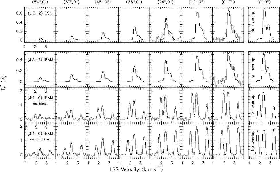
Figure 1: N₂H⁺ observations (grey lines) compared to our best radiative transfer model (see Fig 4a-b). Each column corresponds to a spatial offset (indicated above the top box) from the main dust peak. The top row contains the CSO 10-m data, the other rows the IRAM 30-m data. The (J:1–0) line is split between the bottom row (central triplet) and the next row (’red’ triplet); the isolated ’blue’ component is not shown. The rightmost column represents the fit for the central position with a NLTE code without overlap for the same cloud parameters.

Among the above three species, H₂D⁺ is thus the only one not to deplete. However, it has only one (ortho) transition observable from the ground, that moreover requires excellent sky conditions. The para form ground transition at 1.4 THz should not be detectable in emission in cores with T${}_{\mathrm{kin}}\leq$ 10 K. Therefore H₂D⁺ is useful for chemical and dynamical studies, but brings little information on gas physical conditions. NH₃ inversion lines at 23 GHz can provide kinetic temperature measurements as long as higher lying non-metastable levels are not significantly populated (Walsmley & Ungerechts Walmsley83 (1983)). However, because the critical density of the NH₃ (1,1) inversion line is only $\sim$2000 cm^-3, this tracer may have substantial contribution from external, warmer layers, not representative of the densest parts of PSCs. The third species, N₂H⁺, appears very promising : it has the strong advantage of having mm transitions with critical densities in the range 0.5–70 $\times$ 10⁶ cm^-3 and intense hyperfine components for the (J:1–0) line in typical PSC conditions. The ratio of hyperfine components gives an estimate of the opacity and excitation temperature of the line. Fitting both the hyperfine ratios and the (J:1–0) to (J:3–2) ratio with a rigorous NLTE model should thus bring strong constraints on both T_kin and n(H₂). Collisional coefficients (with He) between individual hyperfine sublevels have become available recently (Daniel et al. Daniel05 (2005)). However, current excitation models (Daniel et al. 2006a ) do not take into account line overlap, which limits their accuracy. Another question that remains is whether N₂H⁺ is indeed able to probe the central core regions, despite the depletion effects which have been reported.

In this paper, we introduce a new NLTE Monte-Carlo 1D code treating N₂H⁺ and N₂D⁺ radiative transfer with line overlap, and apply it to detailed analysis of the main PSC in L183, a clear-cut case of N₂H⁺ depletion (cf. PPABC). We demonstrate the capability of the model to constrain physical conditions inside the PSC (temperature, density profile, abundance and depletion, deuterium fractionation). In particular we show that the gas is very cold at the core center and thermalized with the dust, and that N₂D⁺ appears a very useful tracer of physical conditions in the innermost core regions.

2 Observations and analysis

Table 1: Spectral parameters of each line observed towards the PSC center position ($\alpha$(2000) = 15h54m08.5s, $\delta$(2000)= $-$2°52′48″) with V_LSR = 2.3672(2) km s^-1 (from the NH₃ (1,1) measurement) : noise level, reference observing frequency, intrinsic linewidth of hyperfine transitions and total opacity (both from the CLASS HFS routine), relative velocity and intensity of the main hyperfine groups (from gaussian fits). Values in parentheses are 1$\sigma$ uncertainties on the last digit. For comparison, the T${}_{\mathrm{R}}^{*}$ ratios of hyperfine groups given by their statistical weights are listed in italics. The detailed hyperfine structure of the 3 species is described in Caselli et al. (Caselli95 (1995)) for N₂H⁺, Dore et al. (Dore04 (2004)) for N₂D⁺ and Kukolich (Kukolich67 (1967)) for NH₃

$\begin{array}[]{cccccccccccccccccc}\hline\cr\vskip 3.0pt plus 1.0pt minus 1.0pt\cr&\lx@intercol\hfil\rm{N_{2}H^{+}(J:1-0)}\hfil\lx@intercol&&&\lx@intercol\hfil\rm{N_{2}H^{+}(J:3-2)(IRAM)}\hfil\lx@intercol&&\lx@intercol\hfil\rm{N_{2}H^{+}(J:3-2)(CSO)}\hfil\lx@intercol&\\ \mathrm{Noise\,(1\sigma)\,:}&\lx@intercol\hfil 28\leavevmode\nobreak\ \rm{mK}\hfil\lx@intercol&&&\lx@intercol\hfil 59\leavevmode\nobreak\ \rm{mK}\hfil\lx@intercol&&\lx@intercol\hfil 64\leavevmode\nobreak\ \rm{mK}\hfil\lx@intercol&\\ \mathrm{Ref.\leavevmode\nobreak\ frequency\,:}&\lx@intercol\hfil 93.173764\,\rm{GHz}\hfil\lx@intercol&&&\lx@intercol\hfil 279.511832\,\rm{GHz}\hfil\lx@intercol&&\lx@intercol\hfil 279.511832\,\rm{GHz}\hfil\lx@intercol&\\ \mathrm{Intrinsic\leavevmode\nobreak\ FWHM\,:}&\lx@intercol\hfil 0.195(1)\leavevmode\nobreak\ \rm{km\,s^{-1}}\hfil\lx@intercol&&&\lx@intercol\hfil 0.18(2)\leavevmode\nobreak\ \rm{km\,s^{-1}}\hfil\lx@intercol&&\lx@intercol\hfil{}^{\mathrm{a}}0.28(4)\leavevmode\nobreak\ \rm{km\,s^{-1}}\hfil\lx@intercol&\\ \mathrm{Total\leavevmode\nobreak\ opacity\,:}&\lx@intercol\hfil 21.8(5)\hfil\lx@intercol&&&\lx@intercol\hfil 10(2)\hfil\lx@intercol&&\lx@intercol\hfil 2(1)\hfil\lx@intercol&\\ \vskip 3.0pt plus 1.0pt minus 1.0pt\cr\cline{2-4}\cr\cline{7-9}\cr\cline{11-13}\cr\vskip 3.0pt plus 1.0pt minus 1.0pt\cr\mathrm{Hyperfine}&V_{\mathrm{rel.}}&\rm{T_{R}^{*}}&Area&\lx@intercol\hfil\rm{T^{*}_{R}\leavevmode\nobreak\ Ratio}\hfil\lx@intercol&V_{\mathrm{rel.}}&\rm{T_{R}^{*}}&Area&&V_{\mathrm{rel.}}&\rm{T_{R}^{*}}&Area\\ \mathrm{Group}&\rm{(km\,s^{-1})}&\rm{(K)}&\rm{(K\,km\,s^{-1})}&{\rm obs}&{\rm weights}&\rm{(km\,s^{-1})}&\rm{(K)}&\rm{(K\,km\,s^{-1})}&&\rm{(km\,s^{-1})}&\rm{(K)}&\rm{(K\,km\,s^{-1})}\\ \vskip 3.0pt plus 1.0pt minus 1.0pt\cr\hline\cr\vskip 3.0pt plus 1.0pt minus 1.0pt\cr 1&-8.009(7)&2.05(3)&0.47(3)&0.932&{\it 0.428}&-2.58(1)&0.17(6)&0.013(5)&&-2.63(2)&0.20(6)&0.025(8)\\ 2&-0.611(8)&1.81(3)&0.42(3)&0.822&{\it 0.428}&0.00(1)&0.50(6)&0.29(2)&&0.00(1)&0.67(6)&0.37(2)\\ 3&0.000(7)&2.20(3)&0.60(3)&1&{\it 1}&4.70(8)&2.25(6)&0.014(5)&&4.68(3)&2.12(6)&0.028(9)\\ 4&0.956(7)&2.08(3)&0.54(3)&0.945&{\it 0.714}\\ 5&5.546(7)&2.12(3)&0.47(3)&0.964&{\it 0.428}\\ 6&5.983(8)&2.04(3)&0.53(3)&0.927&{\it 0.714}\\ 7&6.94(1)&1.26(3)&0.24(3)&0.573&{\it 0.143}\\ \vskip 3.0pt plus 1.0pt minus 1.0pt\cr\hline\cr\vskip 3.0pt plus 1.0pt minus 1.0pt\cr&\lx@intercol\hfil\rm{N_{2}D^{+}(J:1-0)}\hfil\lx@intercol&&&\lx@intercol\hfil\rm{N_{2}D^{+}(J:2-1)^{\mathrm{b}}}\hfil\lx@intercol&&\lx@intercol\hfil\rm{N_{2}D^{+}(J:3-2)}\hfil\lx@intercol&\\ \mathrm{Noise\,(1\sigma)\,:}&\lx@intercol\hfil 31\leavevmode\nobreak\ \rm{mK}\hfil\lx@intercol&&&\lx@intercol\hfil 26\leavevmode\nobreak\ \rm{mK}\hfil\lx@intercol&&\lx@intercol\hfil 43\leavevmode\nobreak\ \rm{mK}\hfil\lx@intercol&\\ \mathrm{Ref.\leavevmode\nobreak\ frequency\,:}&\lx@intercol\hfil 77.109616\,\rm{GHz}\hfil\lx@intercol&&&\lx@intercol\hfil 154.217182\,\rm{GHz}\hfil\lx@intercol&&\lx@intercol\hfil 231.321917\leavevmode\nobreak\ \rm{GHz}\hfil\lx@intercol&\\ \mathrm{Intrinsic\leavevmode\nobreak\ FWHM\,:}&\lx@intercol\hfil 0.226\leavevmode\nobreak\ (3)\leavevmode\nobreak\ \rm{km\,s^{-1}}\hfil\lx@intercol&&&\lx@intercol\hfil 0.185\leavevmode\nobreak\ (2)\leavevmode\nobreak\ \rm{km\,s^{-1}}\hfil\lx@intercol&&\lx@intercol\hfil 0.18\leavevmode\nobreak\ (2)\leavevmode\nobreak\ \rm{km\,s^{-1}}\hfil\lx@intercol&\\ \mathrm{Total\leavevmode\nobreak\ opacity\,:}&\lx@intercol\hfil 4.7(3)\hfil\lx@intercol&&&\lx@intercol\hfil 4.9(1)\hfil\lx@intercol&&\lx@intercol\hfil 1.5(7)\hfil\lx@intercol&\\ \vskip 3.0pt plus 1.0pt minus 1.0pt\cr\cline{2-4}\cr\cline{7-9}\cr\cline{11-13}\cr\vskip 3.0pt plus 1.0pt minus 1.0pt\cr&V_{\mathrm{rel.}}&\rm{T_{R}^{*}}&Area&\lx@intercol\hfil\rm{T^{*}_{R}\leavevmode\nobreak\ Ratio}\hfil\lx@intercol&V_{\mathrm{rel.}}&\rm{T_{R}^{*}}&Area&&V_{\mathrm{rel.}}&\rm{T_{R}^{*}}&Area\\ &\rm{(km\,s^{-1})}&\rm{(K)}&\rm{(K\,km\,s^{-1})}&{\rm obs}&{\rm weights}&\rm{(km\,s^{-1})}&\rm{(K)}&\rm{(K\,km\,s^{-1})}&&\rm{(km\,s^{-1})}&\rm{(K)}&\rm{(K\,km\,s^{-1})}\\ \vskip 3.0pt plus 1.0pt minus 1.0pt\cr\hline\cr\vskip 3.0pt plus 1.0pt minus 1.0pt\cr 1&-9.697(8)&0.77(3)&0.15(1)&0.7&{\it 0.428}&-5.35(2)&0.16(3)&0.137(5)&&-3.26(1)&<0.12\\ 2&-0.763(8)&0.76(3)&0.15(1)&0.691&{\it 0.428}&-0.759(8)&0.21(3)&0.080(3)&&0.000(5)&0.72(4)&0.186(8)\\ 3&0.000(7)&1.10(3)&0.33(2)&1&{\it 1}&0.000(1)&1.37(3)&0.513(3)&&0.46(2)&0.19(4)&0.06(1)\\ 4&1.146(8)&0.92(3)&0.25(2)&0.836&{\it 0.714}&0.646(4)&0.40(3)&0.139(3)&&2.47(3)&0.11(4)&0.028(7)\\ 5&6.65(2)&0.55(3)&0.16(2)&0.5&{\it 0.428}&2.5(1)&0.08(3)&0.02(2)&&\\ 6&7.19(1)&0.90(3)&0.23(2)&0.818&{\it 0.714}&2.97(2)&0.43(3)&0.08(2)&&\\ 7&8.34(2)&0.34(3)&0.05(2)&0.309&{\it 0.143}&3.57(5)&0.26(3)&0.16(3)&&\\ \vskip 3.0pt plus 1.0pt minus 1.0pt\cr\hline\cr\vskip 3.0pt plus 1.0pt minus 1.0pt\cr&\lx@intercol\hfil\rm{NH_{3}(1,1)}\hfil\lx@intercol&&&\lx@intercol\hfil\rm{NH_{3}(2,2)}\hfil\lx@intercol\\ \mathrm{Noise\,(1\sigma)\,:}&\lx@intercol\hfil 74\leavevmode\nobreak\ \rm{mK}\hfil\lx@intercol&&&\lx@intercol\hfil 76\leavevmode\nobreak\ \rm{mK}\hfil\lx@intercol&\\ \mathrm{Ref.\leavevmode\nobreak\ frequency\,:}&\lx@intercol\hfil 23.6944957\leavevmode\nobreak\ \rm{GHz}\hfil\lx@intercol&&&\lx@intercol\hfil 23.7226332\leavevmode\nobreak\ \rm{GHz}\hfil\lx@intercol\\ \mathrm{Intrinsic\leavevmode\nobreak\ FWHM\,:}&\lx@intercol\hfil 0.195\leavevmode\nobreak\ (1)\leavevmode\nobreak\ \rm{km\,s^{-1}}\hfil\lx@intercol&&&\lx@intercol\hfil 0.20\leavevmode\nobreak\ (1)\leavevmode\nobreak\ \rm{km\,s^{-1}}\hfil\lx@intercol&\\ \mathrm{Total\leavevmode\nobreak\ opacity\,:}&\lx@intercol\hfil 24.2(4)\hfil\lx@intercol&&&\lx@intercol\hfil 0.1(7)\hfil\lx@intercol\\ \vskip 3.0pt plus 1.0pt minus 1.0pt\cr\cline{2-4}\cr\cline{7-9}\cr\vskip 3.0pt plus 1.0pt minus 1.0pt\cr&V_{\mathrm{rel.}}&\rm{T_{R}^{*}}&Area&\lx@intercol\hfil\rm{T^{*}_{R}\leavevmode\nobreak\ Ratio}\hfil\lx@intercol&V_{\mathrm{rel.}}&\rm{T_{R}^{*}}&Area\\ &\rm{(km\,s^{-1})}&\rm{(K)}&\rm{(K\,km\,s^{-1})}&{\rm obs}&{\rm weights}&\rm{(km\,s^{-1})}&\rm{(K)}&\rm{(K\,km\,s^{-1})}\\ \vskip 3.0pt plus 1.0pt minus 1.0pt\cr\hline\cr\vskip 3.0pt plus 1.0pt minus 1.0pt\cr 1&-19.504(6)&2.62(7)&0.89(4)&0.922&{\it 0.363}&-0.005(5)&0.73(8)&0.152(7)\\ 2&-7.814(5)&2.68(7)&0.69(3)&0.944&{\it 0.273}\\ 3&-7.255(8)&1.95(7)&0.57(3)&0.687&{\it 0.182}\\ 4&-0.17(1)&2.84(7)&1.15(9)&1&{\it 1}\\ 5&0.30(2)&2.78(7)&1.0(1)&0.979&{\it 0.636}\\ 6&7.465(9)&2.60(7)&0.72(5)&0.915&{\it 0.303}\\ 7&7.89(1)&1.91(7)&0.48(5)&0.673&{\it 0.152}\\ 8&19.318(9)&2.48(7)&0.62(4)&0.873&{\it 0.242}\\ 9&19.85(1)&1.72(7)&0.42(5)&0.606&{\it 0.121}\\ \vskip 3.0pt plus 1.0pt minus 1.0pt\cr\hline\cr\end{array}$

• CSO observations are done with a resolution around 0.1 km s^-1 (or more) which explains this larger value

• The hyperfine structure is too complex to be detailed completely. Only the main groups of hyperfine transitions are given

The main dust core in L183 (Pagani et al. Pagani04 (2004)) was observed at the IRAM 30-m telescope in November 2003, July 2004 and October 2006. Spectra were taken on a 12″ grid in an East-West strip across the core (centered at $\alpha$(2000) = 15h54m08.5s, $\delta$(2000)= $-$2°52′48″). Symmetric eastern and western spectra were averaged out to $\pm$ 48″ to give a more representative radial profile. A small anti-symmetric velocity shift of a few tens of m s^-1 was noticed on either sides of the PSC center at distances beyond $\pm$ 30″, possibly indicative of rotation (see Section 3.2). This shift was compensated for when averaging eastern and western spectra, in order not to artificially broaden the lines. Beyond 48″, only eastern positions are considered, as the western side is contaminated by a separate core (Peak 3; Pagani et al. 2004). Lines of N₂H⁺ (J:1–0), (J:3–2) and of N₂D⁺ (J:1–0), (J:2–1) and (J:3–2) were observed in Frequency switching mode, with velocity sampling 30–50 m s^-1 and T_sys ranging from 100 K at 3mm up to 1000 K at 1mm. The N₂H⁺ (J:2–1) line at 186 GHz was not observed, as it lies only 3 GHz away from the telluric water line at 183 GHz, hence its usefulness to constrain excitation conditions would be limited by calibration sensitivity to even tiny sky fluctuations. The problem does not apply to N₂D⁺ which lies a factor of 1.2 lower in frequency. Spatial resolution ranges from 33″ at 77 GHz to 9″ at 279 GHz. Additional CSO 10-m observations of N₂H⁺ (J:3–2) were obtained in June 2004 at selected positions. Observations were done in Position Switch mode with the high resolution AOS (48 kHz sampling) and a T_sys around 600 K. A major interest to observe the (J:3–2) line with the CSO is that the beam size and efficiency is very similar to the 30-m values for the (J:1–0) line, thus almost canceling out beam correction errors in the comparison between the two. It is thus a useful constraint for radiative transfer modelling, even though the higher resolution (9″) 30-m (J:3–2) observations will be essential to constrain abundances and physical conditions in the innermost core regions. Standard reduction techniques were applied using the CLASS reduction package.

Complementary observations of NH₃ (1,1) and (2,2) inversion lines towards the PSC center were also obtained at the new Green Bank 100-m telescope (GBT) in November 2006 with velocity sampling of 20 m s^-1 and a typical T_sys of 50 K, in Frequency Switch mode. The angular resolution ($\sim$35″) is close to that of the 30-m in the low frequency (J:1-0) N₂D⁺line. The main beam efficiency of the GBT at 23 GHz is between 0.95 and 1, hence no correction was applied to put the spectra on T${}_{\mathrm{R}}^{*}$ scale.

Table 1 summarizes the main observational parameters of the lines observed towards the core center : noise level of the spectrum (rms), rotational line total opacity and intrinsic FWHM width of individual hyperfine transitions (as fitted by the CLASS HFS routine, which assumes equal excitation temperature for all sublevels), and relative velocity centroids and intensities of the main hyperfine groups in our spectra (derived from gaussian fits). Note that the hyperfine groups are always broader than the intrinsic linewidth derived by CLASS, due to optical depth effects and/or to the presence of adjacent hyperfine components too close to be spectroscopically separated.

To compare with models, beam efficiency correction is an important issue. Since L183 (as well as other PSCs) is very extended compared to the primary beam of 10″–30″, the T_mb intensity scale is inadequate, as it will overcorrect for source-antenna coupling and thus overestimate the true source surface brightness (cf. PPABC). To avoid this problem, observed spectra are corrected only for moon efficiency ($\sim$ T${}_{\mathrm{R}}^{*}$ scale), while models are convolved by the full beam pattern of the 30m telescope (cf. Greve et al. Greve98 (1998)), yielding intensities on the same T${}_{\mathrm{R}}^{*}$ scale. For the CSO, we also correct the data for moon efficiency ($\eta_{\mathrm{moon}}$ $\approx$ 0.8 at 279 GHz) and as the details of the beam pattern are not known, the model output is convolved with a simple gaussian beam. Because the CSO main beam coupling is very good at 1.1 mm ($\eta_{\mathrm{MB}}\geq$ 0.7), the uncertainty of the correction should be limited.

In order to treat correctly the beam coupling to the source, we also take into account the fact that the L183 core is located within a larger-scale N₂H⁺ filament oriented roughly north-south, as revealed by previous low resolution maps (PPABC). This elongation is mostly constant in intensity over $\simeq$ 6 arcminutes. Therefore we approximate the brightness distribution as a cylinder of length 6′, with its axis in the plane of the sky. The intensity distribution along the east-west section of the cylinder is taken as the emergent signal along the equator of our spherical Monte-Carlo model. We then replicate these values along the (north-south) cylinder axis before convolving by the antenna beam. For N₂D⁺, the (unpublished) large-scale map shows a smaller north-south extent ($\simeq$ 2′) hence we use a cylinder length of 2′ for convolving our model.

In Figs. 1 and LABEL:n2dp, we plot the observations in T${}_{\mathrm{R}}^{*}$ compared to our best model (see Section  3.4), convolved by the antenna beam as explained above.

3 Modelling and discussion

3.1 Radiative transfer code

Our spherical Monte-Carlo code is derived from Bernes’ code (Bernes Bernes (1979)) and has been extensively tested on models of CO emission from dense cores (e.g. Pagani Pagani98 (1998)). It was recently updated to take into account overlap between hyperfine transitions occuring at close or identical frequencies. This is done by treating simultaneously the photon transfer for all hyperfine transitions of the same rotational line (see also Appendix in Gónzalez-Alfonso & Cernicharo Gonzalez93 (1993)). Instead of choosing randomly the frequency of the emitted photon, a binned frequency vector is defined for each rotational transition inside which all hyperfine transitions are positioned. All bins are filled with their share of spontaneously emitted photons (or 2.7 K continuum background photons) and, during photon propagation, absorption is calculated for each bin by summing all the hyperfine transition opacities at that frequency

$$\tau(\nu)=\int\kappa(\nu)\mathrm{d}s=\sum_{i}\tau_{i}\phi_{i}(\nu)=\int\left(\sum_{i}\kappa_{i}\phi_{i}(\nu)\right)\mathrm{d}s$$

where $\kappa_{i}$ is the absorption coefficient, $\tau_{i}$ the opacity and $\phi_{i}(\nu)$ the local frequency profile of the i^th hyperfine transition. The total number of absorbed photons I${}_{o}(\nu)e^{-\tau(\nu)}$ is then redistributed among hyperfine levels according to their relative absorption coefficients

$$\mathrm{d}I_{i}(\nu)=\frac{\kappa_{i}\phi_{i}(\nu)}{\kappa(\nu)}\times I_{o}(\nu)e^{-\tau(\nu)}$$

Overlap is treated for all rotational transitions. Statistical equilibrium, including collisions, is then solved separately for each hyperfine energy level.

Collisional coefficients are available for transitions between all individual hyperfine levels, but were calculated with He as a collisioner instead of H₂ (Daniel et al. Daniel05 (2005)). We scaled them up by 1.37 to correct for the difference in reduced mass, but note that this correction is only approximate (see Willey et al. Willey02 (2002) and Daniel et al. 2006a ). The code works for both isotopologues. As one can probably neglect the variation of the electric dipole moment (Gerin et al. Gerin01 (2001)), the N₂D⁺ Einstein spontaneous emission coefficients are derived from those of N₂H⁺ by simply scaling them down by 1.2³. Deexcitation collisional coefficients are kept the same as for N₂H⁺ (following Daniel et al. 2006b ).

The local line profile in our 1D code takes into account both thermal and turbulent broadening, as well as any radial and rotational velocity fields. In principle, rotation introduces a deviation from spherical symmetry. However, for small rotational velocities (less than half the linewidth, typically), the excitation conditions do not noticeably change within a given radial shell, as shown by a previous 2–D version of this code (Pagani & Bréart de Boisanger, Pagani96 (1996)). Therefore the (much faster) 1D version remains sufficiently accurate.

Our Monte-Carlo model shows that excitation temperatures among individual hyperfine transitions within a given rotational line differ by up to 15 %, hence the usual assumption of a single excitation temperature to estimate the line opacity (e.g. in the CLASS HFS routine) is not fully accurate as already noticed by Caselli et al. (Caselli95 (1995)). Neglecting line overlap affects differentially the excitation temperature of hyperfine components when the opacity is high enough, mostly decreasing it, but also increasing it in a few cases. For example, in our best model for the L183 PSC, the excitation temperatures of individual hyperfine components change by up to 10%. As shown in the last column of Fig. 1, a noticeable difference between models with and without overlap appears in the (J:3–2) line shape.

3.2 Grid of models

Table 2: The 4 main density laws investigated in our models, and the corresponding temperature and abundance profiles giving the best fit to N₂H⁺ data in each case. The leftmost model gave the best overall fit (see Table 3) and was used to compute the synthetic spectra in Figs. 1 and 2. Its best N2D+ abundance profile is also listed. Parameters are held constant inside a given radial shell, except for the rotational speed which is linearly interpolated. 2.34(6) reads 2.34 $\times$ 10⁶.

$\begin{array}[]{cccccccccccccccccc}\hline\cr\vskip 3.0pt plus 1.0pt minus 1.0pt\cr&&\lx@intercol\hfil\rho\propto r^{-1},r^{-2}\,(\rm{Best\leavevmode\nobreak\ model})^{\mathrm{a}}\hfil\lx@intercol&&\lx@intercol\hfil\rho\propto r^{-1}\hfil\lx@intercol&&\lx@intercol\hfil\rho\propto r^{-1.5}\hfil\lx@intercol&&\lx@intercol\hfil\rho\propto r^{-2}\hfil\lx@intercol\\ \vskip 3.0pt plus 1.0pt minus 1.0pt\cr\cline{3-6}\cr\cline{8-10}\cr\cline{12-14}\cr\cline{16-18}\cr\vskip 3.0pt plus 1.0pt minus 1.0pt\cr\rm{Radius}&\rm{V.\leavevmode\nobreak\ rot.}&\rm{Density}&T_{\mathrm{kin}}&\rm{Abundance}&\rm{Abundance}&&\rm{Density}&T_{\mathrm{kin}}&\rm{Abundance}&\nobreak\leavevmode\hfil&\rm{Density}&T_{\mathrm{kin}}&\rm{Abundance}&\nobreak\leavevmode\hfil&\rm{Density}&T_{\mathrm{kin}}&\rm{Abundance}\\ \rm{A.U.}&\rm{(km\,s^{-1})}&\rm{(cm^{-3})}&\rm{(K)}&\rm{N_{2}H^{+}}&\rm{N_{2}D^{+}}&&\rm{(cm^{-3})}&\rm{(K)}&\rm{N_{2}H^{+}}&\nobreak\leavevmode\hfil&\rm{(cm^{-3})}&\rm{(K)}&\rm{N_{2}H^{+}}&\nobreak\leavevmode\hfil&\rm{(cm^{-3})}&\rm{(K)}&\rm{N_{2}H^{+}}\\ \vskip 3.0pt plus 1.0pt minus 1.0pt\cr\hline\cr\vskip 3.0pt plus 1.0pt minus 1.0pt\cr 330&0&2.34(6)^{\mathrm{b}}&7&2.4(-11)&2(-11)&&2.34(6)^{\mathrm{b}}&7&7(-11)&&3.30(6)^{\mathrm{c}}&7&1(-11)&&3.46(6)^{\mathrm{c}}&9&1(-11)\\ 660&0&2.05(6)^{\mathrm{b}}&7&2.4(-11)&2(-11)&&2.05(6)^{\mathrm{b}}&7&7(-11)&&2.89(6)^{\mathrm{c}}&7&1(-11)&&3.03(6)^{\mathrm{c}}&9&1(-11)\\ 990&0&1.55(6)^{\mathrm{b}}&7&8.5(-11)&4(-11)&&1.55(6)^{\mathrm{b}}&7&7(-11)&&2.19(6)^{\mathrm{c}}&7&7(-11)&&2.29(6)^{\mathrm{c}}&9&3(-11)\\ 1320&0&1.16(6)&7&8.5(-11)&4(-11)&&1.16(6)&7&7(-11)&&1.19(6)&7&7(-11)&&1.46(6)&9&3(-11)\\ 1650&0&9.27(5)&7&8.5(-11)&4(-11)&&9.27(5)&7&7(-11)&&7.74(5)&7&7(-11)&&9.09(5)&9&3(-11)\\ 1980&0&7.73(5)&7&8.5(-11)&4(-11)&&7.73(5)&7&7(-11)&&5.55(5)&7&7(-11)&&6.10(5)&9&3(-11)\\ 2310&0&6.62(5)&7&1.1(-10)&3(-11)&&6.62(5)&7&1(-10)&&4.20(5)&7&4(-10)&&4.39(5)&9&1(-10)\\ 2640&0&5.80(5)&7&1.1(-10)&3(-11)&&5.80(5)&7&1(-10)&&3.34(5)&7&4(-10)&&3.54(5)&9&1(-10)\\ 2970&0&5.15(5)&7&1.1(-10)&3(-11)&&5.15(5)&7&1(-10)&&2.74(5)&7&4(-10)&&2.68(5)&9&1(-10)\\ 3300&0.01&4.64(5)&7&1.1(-10)&3(-11)&&4.64(5)&7&1(-10)&&2.29(5)&7&4(-10)&&2.20(5)&9&1(-10)\\ 3630&0.01&4.21(5)&7&1.5(-10)&3(-11)&&4.21(5)&7&1.5(-10)&&1.95(5)&7&3(-10)&&1.83(5)&9&6(-10)\\ 3960&0.01&3.54(5)&7&1.5(-10)&3(-11)&&3.86(5)&7&1.5(-10)&&1.70(5)&7&3(-10)&&1.46(5)&9&6(-10)\\ 4290&0.02&3.01(5)&7&1.5(-10)&3(-11)&&3.57(5)&7&1.5(-10)&&1.49(5)&7&3(-10)&&1.22(5)&9&6(-10)\\ 4620&0.02&2.60(5)&7&1.5(-10)&3(-11)&&3.31(5)&7&1.5(-10)&&1.32(5)&7&3(-10)&&1.07(5)&9&6(-10)\\ 4950&0.02&2.26(5)&7&1.3(-10)&5(-12)&&3.09(5)&7&5(-11)&&1.18(5)&7&3(-10)&&9.27(4)&9&4(-10)\\ 5280&0.05&1.99(5)&7&1.3(-10)&5(-12)&&2.90(5)&7&5(-11)&&1.07(5)&7&3(-10)&&8.5(4)&9&4(-10)\\ 5610&0.05&1.76(5)&7&1.3(-10)&5(-12)&&2.73(5)&7&5(-11)&&9.67(4)&7&3(-10)&&7.20(4)&9&4(-10)\\ 5940&0.05&1.57(5)&8&1.3(-10)&5(-12)&&2.58(5)&8&5(-11)&&8.82(4)&7&3(-10)&&6.34(4)&9&4(-10)\\ 6667&0.05&1.27(5)&8&1(-10)&\leq 4(-12)&&2.02(5)&8&2.5(-11)&&8.10(4)&7&1.5(-10)&&5.25(4)&9&4(-10)\\ 7733&0.05&8.50(4)&9&1(-10)&\leq 4(-12)&&1.57(5)&9&2.5(-11)&&6.77(4)&7&1.5(-10)&&4.55(4)&9&4(-10)\\ 8867&0.05&6.50(4)&10&1(-10)&\leq 4(-12)&&8.50(4)^{\mathrm{d}}&10&2.5(-11)&&5.42(4)&7&1.5(-10)&&3.46(4)&9&4(-10)\\ 10000&0.02&5.20(4)&11&1(-10)&\leq 4(-12)&&5.20(4)^{\mathrm{d}}&11&2.5(-11)&&4.41(4)&7&1.5(-10)&&2.68(4)&9&4(-10)\\ 13333&0&3.45(4)&12&1(-10)&\leq 4(-12)&&3.45(4)^{\mathrm{d}}&12&2.5(-11)&&3.68(4)&7&1.5(-10)&&1.70(4)&9&4(-10)\\ \vskip 3.0pt plus 1.0pt minus 1.0pt\cr\hline\cr\end{array}$

• $\rho\propto$ r^-1 (r $<$ 4000 AU), $\rho\propto$ r^-2 (r $>$ 4000 AU)

• The first three layer densities do not follow a power law but the density profile derived from the ISOCAM absorption map (Pagani et al. Pagani04 (2004))

• Same as note (b) above, but rescaled to maintain a constant total column density of 1.4$\times$ 10²³ cm^-2 (see text).

• For the pure $\rho\propto$ r^-1 case, density is not falling off fast enough to reach ambient cloud density and we correct for this in the last 3 layers.

Our core model has an outer radius of 13333 AU $\simeq$ 2′, fixed by the maximum width $\simeq$ 4′of detectable N₂H⁺ emission in the east-west direction across the PSC, as seen in large scale maps (PPABC). We assume that N₂H⁺ abundance is zero outside of this radius (due to chemical destruction by CO).

For all models, the microscopic turbulence is set to $\Delta$v_turb(FWHM) = 0.136 km s^-1. This was found sufficient to reproduce the width of individual hyperfine groups, and is comparable to the thermal width contribution. A small rotational velocity field of a few tens of m s^-1 was further imposed beyond 3000 AU (see Table 2) to reproduce the small anti-symmetric velocity shift from PSC center observed at distances beyond $\pm$ 30″ (cf. Section 2). The radial velocity was kept to 0 in all layers. As seen in Figs. 1 and 2, this approximation already gives a remarkable fit to observed line profiles, and is therefore sufficient to derive the overall temperature and abundance structure.

We considered a variety of density profiles: single power law profiles $\rho\propto$ r^-1, $\rho\propto$ r^-1.5, $\rho\propto$ r^-2, as well as broken power laws with $\rho\propto$ r^-1 out to 4000 AU followed by r^-2, or by r^-3.5. For good accuracy, the density profile was sampled in 330 AU = 3″ thick shells, i.e. 3 to 10 times smaller than our observational beam sizes. In all cases, divergence at $r=0$ was avoided by adopting inside r = 990 AU the density slope derived from the ISOCAM data (Pagani et al. 2004). The density profiles were then scaled to give the same total column density N(H₂) = 1.4 $\times$ 10²³ cm^-2 towards the PSC center, as estimated from the MAMBO emission map (Pagani et al. 2004). The effect of changing the total N(H₂) on the fit results will be discussed in Section 3.4.1.

We then considered a variety of temperatures spanning the range 6–10 K in the inner core regions. We also tested non-constant temperature laws, increasing up to 12 K in the outermost layers and/or in the innermost layers.

For each combination of density and temperature laws, a range of N₂H⁺ abundance profiles was investigated. To avoid a prohibitive number of cases, abundances were sampled in 6 concentric layers only, corresponding to the spatial sampling of our spectra (except the last, wider layer which encompasses the outermost two offsets), and multiple maxima/minima were forbidden. This lead to a total of about 40,000 calculated models with 8 free parameters (6 abundances, 1 temperature profile, 1 density profile). Table 2 lists the values of H₂ densities for 4 density laws, together with the temperature and abundance profiles that best fitted the data in each case (cf. next section).

3.3 Selection criteria

Figure 3: Global $\chi^{2}_{\nu}$ for all density profiles and temperature cases. An arrow indicates that the majority of the model layers is at the given temperature but that outer layers have rising temperatures. Only one (circled) solution satisfies all 4 individual $\chi^{2}$ fitting (see text)

Our best fit selection criteria are based on the use of several $\chi^{2}$ and (reduced) $\chi^{2}_{\nu}$ estimates. Because the N₂H⁺ (J:1–0) data have much more overall weight than the (J:3–2) data (more isolated hyperfine groups per spectrum, more observed positions, higher signal-to-noise ratio), computing a single $\chi^{2}_{\nu}$ per model is hardly sensitive to the quality of the (J:3–2) line fit. However, the (J:1–0) spectra being optically thick, they give little constraints on the temperature and N₂H⁺ abundance of the innermost layers (within a 6″ radius). Those are only constrained by the IRAM (J:3–2) observations. The CSO (J:3–2) spectrum at (24″,0″) also adds interesting information on the density profile.

To constrain the models we thus evaluate the goodness of fit independently for the (J:1–0) and (J:3–2) data, by computing $\chi^{2}$ values on 4 types of measurements : 1) full area of each of the 7 (J:1–0) hyperfine components, at each of the 7 offset positions (49 values). This measurement is sensitive to the global temperature and abundance profiles. Fitting separately each hyperfine component allows to discard solutions with overall identical area but different hyperfine line ratios; 2) area of the 5 central channels (= 0.15 km s^-1) of each hyperfine component for the same lines (49 values), in order to reject self-absorbed profiles, i.e. line profiles which have the same total area but are wider and self-absorbed; 3) total area of the (J:3–2) CSO spectrum at (24″,0″) (1 value). This single measurement helps to constrain the density profile; 4) total area of the (J:3-2) 30-m spectrum (1 value) which constrains the abundance (and the temperature to some extent) at the core center. These four measurements are of course not completely independent from each other, and trying to improve one fit by changing a model parameter can degrade one or several of the others. We used $\chi^{2}_{\nu}$ for the first two (with 41 degrees of freedom) and $\chi^{2}$ for the last two (only one measurement) so that in all cases $\Delta\chi^{2}\approx$ 1 is equivalent to a 1$\sigma$ deviation. With this choice, a 3$\sigma$ variation is equivalent to $\Delta\chi^{2}_{\nu}\approx$ 1.5 for the first two and $\Delta\chi^{2}$ = 9 for the last two.

After having run all of the models in our grid, we first used a single, global $\chi^{2}_{\nu}$ combining the four types of measurements to visualize the global fit quality of the various models. Fig. 3 plots the global $\chi^{2}_{\nu}$ as a function of temperature, for the various density laws that we investigated. Symbols with arrows indicate models where temperature rises in the outermost layers. For each density-temperature pair, we plot only the smallest $\chi^{2}_{\nu}$ obtained by adjusting the abundance profile.

It is readily seen that the best fits are found for relatively low overall core temperatures $\simeq$ 6.5–8 K. Hence, the (J:1–0) data alone (which dominate the global $\chi^{2}_{\nu}$) set a strong constraint on the core temperature : indeed, the combination of strong opacity and relatively low intensity in this line requires low excitation temperature. Because the (J:1–0) line should be thermalized in the dense center, this rules out kinetic temperatures above 8 K (for our adopted total column density of 1.4$\times$ 10²³ cm^-2).

To further discriminate among models, we then looked individually at the four quality indicators described above, in particular those related to the (J:3-2) lines. Table 3 lists these 4 values as well as the global $\chi^{2}_{\nu}$ for various models selected from Fig. 3, namely: the best model fits for a given constant core temperature (from 6 to 10 K), and the best model fits for a given density law (with corresponding temperature and abundance distributions given in Table 2).

Table 3: Quality of fit evaluated individually on four different sets of measurements, and global $\chi_{\nu}^{2}$, for selected models from Fig. 3 (see text). A difference of 1 corresponds to 1$\sigma$ in all cases. Values for the best model are in bold face. The last rows show the effect of changing only the central N₂H⁺ abundance in this best model

		(J:1–0)			(J:3–2)
model parameters		Total area $\chi^{2}_{\nu}$	5 channels area $\chi^{2}_{\nu}$		CSO Total area $\chi^{2}$	IRAM Total area $\chi^{2}$	Global $\chi^{2}_{\nu}$
Best fit for each temperature (adjusted in abundance)
T = 6 K	($\rho\propto$ r-1,r-2)	4.7	3.8		1.5	1.0	3.9
T = 7 K	($\rho\propto$ r-1,r-2)	1.9	2.4		12.6	4.1	2.1
T = 8 K	($\rho\propto$ r-1.5)	3.1	3.2		0.2	3.4	2.9
T = 9 K	($\rho\propto$ r-2)	4.5	5.6		7.5	6.8	4.7
T = 10 K	($\rho\propto$ r-2)	4.8	6.3		16.9	28.7	5.5
Best fit for each density law (adjusted in abundance)
$\rho\propto$ r-1,r-2	(T = 7 $\rightarrow$ 12 K)	2.4	2.7		0.3	0.0	2.3
$\rho\propto$ r-1	(T = 7 $\rightarrow$ 12 K)	3.7	3.8		1.2	2.9	3.4
$\rho\propto$ r-1.5	(T = 7 K)	3.4	3.2		0.1	0.1	2.9
$\rho\propto$ r-2	(T = 9 K)	4.5	5.6		7.5	6.8	4.7
Varying the central N2H+ abundance at r $<$ 660 AU in the best model
X(N2H+) =	10-12	2.6	2.8		0.3	2.0	2.5
X(N2H+) =	8 $\times$ 10-12	2.6	2.8		0.3	1.0	2.5
X(N2H+) =	2.4 $\times$ 10-11	2.4	2.7		0.3	0.0	2.3
X(N2H+) =	8 $\times$ 10-11	2.1	2.4		0.5	9.2	2.1

It can be seen in Table 3 that for T_kin = 10 K the (J:3–2) lines are not well fitted (4 and 5 $\sigma$ deviations for the CSO and IRAM lines respectively), hence such a high temperature seems ruled out here. Overall, it is rather difficult to have low $\chi^{2}$ values in both the (J:1-0) and the (J:3-2) indicators. Only one density-temperature combination (indicated by bold faces in Table 3) reaches low values in all 4 individual $\chi^{2}_{\nu}$ and $\chi^{2}$, each within 1$\sigma$ of their minimum value, among all the models in Table 3. This combination is referred to as our “best model” in the following, and its inferred physical parameters are discussed in the next section. It can also be noticed in Table 3 that the model with T_kin = 7 K has a slightly better global $\chi^{2}_{\nu}$ than the best model (2.1 compared to 2.3) but is to be eliminated as the (J:3–2) lines are 2 and 3.5 $\sigma$ off the mark.

3.4 Physical conditions in the L183 main core

3.4.1 Density and temperature structure

Our best density-temperature combination (circled 5-branch star symbol in Fig. 3) has a density law of r^-1 out to r $\approx$ 4000 A.U., consistent with the ISOCAM profile (Pagani et al. 2004) and a slope of r^-2 beyond. The temperature is constant at 7 K out to 5600 A.U. and increases up to 12 K at the core edge (see Table 2). Further increasing the number of warmer layers failed, as well as introducing warmer layers in the center. Keeping the temperature constant at 7 K everywhere significantly worsens the fit of the (J:3–2) lines (see Table 3).

The main uncertainty in our temperature determination stems from the assumed total gas column density through the core. Decreasing/increasing it by a factor 1.4 (the typical uncertainty found by Pagani et al. 2004) changes all volume densities by the same factor. To recover the same N₂H⁺ emission, we find that the kinetic temperature in our models must be increased/decreased by $\simeq$1 K (respectively, while the N₂H⁺ abundance must be scaled accordingly to keep the same column density). Since the dust temperature in the L183 core is 7.5 $\pm$ 0.5 K (Pagani et al. 2004), gas and dust are thermalized inside this core within the uncertainties.

A different result was found by Bergin et al. (Bergin06 (2006)) in the B68 PSC, where outer layers emitting in CO are consistent with a kinetic temperature of 7–8 K while NH₃ measurements indicate a higher temperature of 10–11 K in the inner 40″. This inward increase in gas temperature was attributed to the lack of efficient CO cooling in the depleted core center, and requires an order of magnitude reduction in the gas to dust coupling, possibly due to grain coagulation (Bergin et al. Bergin06 (2006)). Such an effect is not seen in L183, despite strong CO depletion within the inner 1′= 6600 AU radius. Our best fit temperature law is more consistent with the thermo-chemical evolution of slowly contracting prestellar cores with standard gas-dust coupling coefficients, which predicts low gas temperatures $\simeq$ 6 K near the core center, increasing to $\simeq$ 14 K near the core surface (Lesaffre et al. lesaffre (2005)).

3.4.2 N₂H⁺ abundance profile

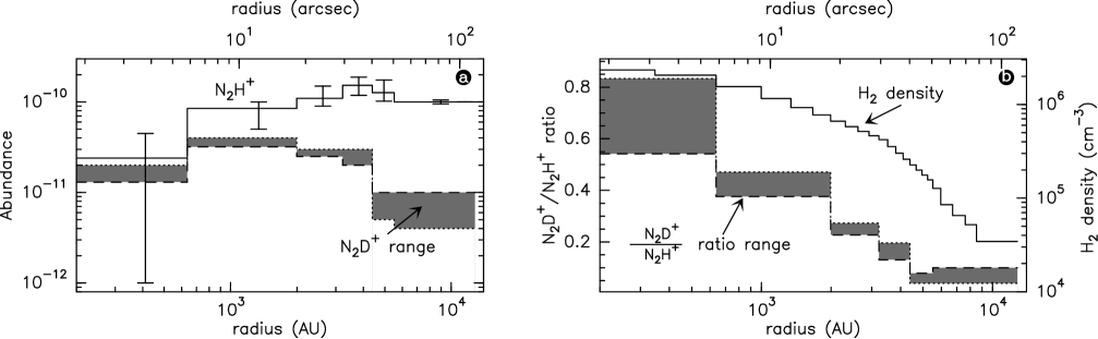
Figure 4: a N₂D⁺ and N₂H⁺ abundances for the best model. For N₂H⁺, the median abundance profile is plotted (the corresponding model output is displayed in Fig. 1). Error bars indicate the range of possible values (see text). For N₂D⁺, a range of values is given: The upper, dotted histogram gives the best fit to the (J:2-1) and (J:3-2) lines, and was used to compute the model in Fig. 2. The dashed histogram gives the best fit to the (J:1-0) and (J:2-1) lines. b density profile of the best model and N₂D⁺/N₂H⁺ ratio range

With our best density-temperature model, several N₂H⁺ abundance profiles give equally good fits (within $<$1$\sigma$ on all 4 quality indicators). From all these acceptable abundance profiles, we determined a median profile (plotted as a solid histogram in Fig. 4a), with error bars representing the range of acceptable values in each layer (though not any combination of these values does fit the observations). This median profile, whose values are listed in Table 2, is used to compute the fit displayed in Fig. 1. The total N₂H⁺ column density is 1.2$\pm 0.1$ $\times$ 10¹³ cm^-2, comparable with the value reported by Dickens et al. (Dickens (2000)) and a factor of $\sim$2 below that in Crapsi et al. (Crapsi05 (2005)).

The maximum N₂H⁺ abundance is 1.5${}_{-0.3}^{+0.4}$ $\times$ 10^-10, the same as found by Tafalla et al. (Tafalla04 (2004)) in L1498 and L1517. However, there is a definite drop in abundance in the inner layers. This drop is imposed by the fit to the (J:3–2) IRAM central spectrum (9″ beam), which is quite sensitive to variations in the central abundance of N₂H⁺, as illustrated in the last rows of Table 3. In contrast, the (J:1–0) line is optically thick at the core center and the $\chi_{\nu}^{2}$ is thus not sensitive to this parameter (cf. Table 3).

Exploring a broad range of abundance profiles, we find only a limited range of possible N₂H⁺ abundances in the inner layer of 6″ radius (r $<$ 660 AU): values above 4.5 $\times$ 10^-11 always produce too strong (J:3–2) emission in the central IRAM beam ($\chi^{2}>1$), while abundances below 10^-12 give a (J:3–2) line marginally too weak. We thus derive a range of 2.4 ${}^{+2.1}_{-2.3}$ $\times$ 10^-11 for the central N₂H⁺ abundance. However, we note that our results for N₂D⁺ would favor a value of at least 10^-11 (see next section).

Compared with the maximum abundance, this gives a volume depletion factor of $\simeq$ 6${}^{+13}_{-3}$ at the core center. The median abundance drop is less than (but marginally consistent with) that expected from simple geometrical arguments in PPABC, but it confirms that the leveling of N₂H⁺ intensity seen across the dust peak is not due to pure opacity effects. As can be seen from Fig. 4a-b, depletion starts at a density of 5–7 $\times$ 10⁵ cm^-3 and increases as density goes up, in agreement with the conclusions of PPABC. The abundance also drops slightly in the outermost regions, possibly due to partial destruction by CO. Indeed, the outermost layers of the model have densities of a few 10⁴ cm^-3 which is the limit above which CO starts to deplete in this source (PPABC).

3.4.3 N₂D⁺ abundance profile

As seen in Fig.LABEL:n2dp, good fits to the N₂D⁺ data may be obtained with the same density and temperature profile as our best model for N₂H⁺, although it is difficult to reproduce simultaneously the intensities of both (J:1-0) and (J:3-2) lines. We plot in Fig. 4a the N₂D⁺ abundance profiles giving the best fit either for (J:1-0) and (J:2-1) (dashed histogram) or for (J:2-1) and (J:3-2) (dotted histogram). The latter was used to produce Fig. LABEL:n2dp. A better fit could be obtained with a temperature of 8 K instead of 7 K. This might indicate that the collisional coefficients with He are somewhat inaccurate to represent those with H₂. Indeed, it has been shown for NH₃ that collisional coefficients with He could differ by a factor up to 4 with respect to those computed with para-H₂ (Willey et al. Willey02 (2002)). A similar problem may occur here (see also the discussion in Daniel et al. 2006a ). Therefore we consider that the temperatures are compatible within the uncertainties on the collisional coefficients.

The N₂D⁺ abundance profile is quite different from that of N₂H⁺ (cf. Fig. 4a). Its abundance is essentially an upper limit beyond 6000 A.U. It increases sharply by about an order of magnitude in the region between 600 and 4000 A.U., then slightly drops by a factor of 2–2.5 in the core center, reaching an abundance between 1.3 and 2 $\times$ 10^-11. The low optical depth of the line ($\tau$ = 0.84 for the strongest hyperfine component, J_FF′:1₂₃–0₁₂) allows to measure the contribution of all layers to the emission and to determine with relatively little uncertainty the abundance profile. In particular, for the chosen density and temperature profiles, we find that the abundance of N₂D⁺ in the center of the cloud cannot be below 10^-11. Hence, we can set tighter constraints on the N₂D⁺ abundance at the core center than was possible for N₂H⁺.

The N₂D⁺/N₂H⁺ ratio obtained by comparing the N₂D⁺ range of abundances to the median N₂H⁺ abundance profile is plotted in Fig. 4b. The deuteration ratio varies from an upper limit $\leq$0.05–0.1 away from the core to a very high factor of 0.7$\pm$0.12 in the depletion region. This is larger than what Tine et al. (Tine (2000)) reported 48″ further north in the same source, and 3–4 times larger than what Crapsi et al. (Crapsi05 (2005)) report towards the PSC. Deuterium enrichment is thus very strong and can certainly be linked to the strong and extended H₂D⁺ line detected towards this source (Vastel et al. Vastel06 (2006)). If we consider the full range of possible values for N₂H⁺ itself, the deuteration ratio in the inner layer ranges from $\sim$0.3 to $\geq$ 20. However, as D₂H⁺ has not been detected in this source despite its strong H₂D⁺ line (Vastel et al. Vastel06 (2006)), an enrichment above 1 seems unprobable, suggesting that the central abundance of N₂H⁺ is probably at least 10^-11.

3.5 Comparison with NH₃ temperature estimates

The low kinetic temperatures $\leq$8 K inferred from our N₂H⁺ and N₂D⁺ modelling are somewhat lower than previous temperature estimates in L183 from NH₃ inversion lines, which gave values in the range 9–10 K (Ungerechts et al. Ungerechts80 (1980), Dickens et al. Dickens (2000)) up to 12 K (Swade et al. Swade89 (1989)). However, these NH₃ spectra were not obtained towards the PSC center itself, and had relatively low angular resolution for the last two. We thus briefly reconsider this issue using our NH₃ spectra obtained at the PSC center position, which also benefit from the higher resolution and beam coupling of the new GBT. The NH₃ spectra were analyzed in the standard way, as discussed by Ho & Townes (Ho83 (1983)) and Walmsley & Ungerechts (Walmsley83 (1983)). Using the CLASS NH3 fitting procedure, we found a total opacity of 24 for the (1,1) inversion line, and an excitation temperature of 5.5 K assuming a beam filling-factor of 1 (Figs. 5 & 6). Making the usual assumption of constant temperature on the line of sight and of negligible population in the non-metastable levels, the intensity ratio of the (2,2) to (1,1) main lines indicates a rotation temperature of 8.4 $\pm$0.3 K which should correspond to a kinetic temperature of 8.6 $\pm$0.3 K. Hence, NH₃ emission towards the PSC center indicates an only slightly higher kinetic temperature than N₂H⁺ (8.6 $\pm$0.3 K instead of 7 $\pm$1 K), almost equal to that obtained with N₂D⁺ ($\sim$8 K). The discrepancy between NH₃ and N₂H⁺ is thus not as large as originally thought. Both tracers point to very cold gas in the core, close to thermal equilibrium with the dust.

Figure 5: GBT NH₃ (1,1) inversion line towards the reference position with CLASS NH3 fit (shifted by +3 K for clarity) and fit residual (shifted by -0.6 K). The fit yields a total opacity of 24.2 ($\pm$0.4), and a global velocity of 2.3672 ($\pm$0.0002) km s^-1

Figure 6: GBT NH₃ (2,2) inversion line towards the reference position. A gaussian fit to the main line indicates a velocity of 2.362 ($\pm$0.005) km s^-1

Reasons for a possible difference between NH₃ and N₂H⁺ temperature determinations in L183 include the following : 1) the higher sensitivity of NH₃ to the warmer outer layers of the core, since NH₃ inversion lines are much easier to thermalize (n${}_{\mathrm{crit}}\approx$ 2000 cm^-3) than N₂H⁺ lines. 2) a slight overestimate in the total column density towards the PSC (reducing it to 10²³ cm^-2, the temperature has to be raised to 8 K to compensate for the density decrease and recover the same N₂H⁺ emission). 3) systematic errors introduced by the use of collisional coefficients with He instead of H₂ for N₂H⁺ (see Sect. 3.4.3). 4) concerning NH₃, standard hypotheses leads to a puzzling discrepancy between T_ex = 5.5 K and T_rot = 8.4 K towards the L183 PSC center, where NH₃ inversion lines should be fully thermalized. Beam dilution has been invoked for giant molecular clouds (thus increasing T_ex), but it seems unreasonable to extend this to dense cloud cores (Swade Swade89 (1989), and references therein). A Monte-Carlo code (or equivalent) would be needed to model NH₃ taking into account the strong density gradients present in PSCs, and the possible population of non-metastable levels at very high densities.

4 Conclusions

1. We have presented a new Monte-Carlo code (available upon request to the author) to compute more realistically the NLTE emission of N₂H⁺ and N₂D⁺, taking into account both line overlap and hyperfine structure. This code may be used to infer valuable information on physical conditions in PSCs.

2. The best kinetic temperature to explain N₂H⁺ observations of the L183 main core is 7$\pm$1 K (and $\sim$ 8 K for N₂D⁺) inside 5600 AU, therefore gas appears thermalized with dust in this source.

3. There is no major discrepancy with NH₃ measurements which also indicate very cold gas (8.6 $\pm$0.3 K) towards the PSC.

4. We have found a noticeable depletion of N₂H⁺ by a factor of 6${}^{+13}_{-3}$, and of N₂D⁺ by a smaller factor of 2–2.5. This smaller depletion is probably due to a strong (0.7$\pm$0.12) deuterium fractionation, consistent with the detection of H₂D⁺ in this core.

5. N₂D⁺ should be a useful probe of the innermost core regions, thanks to its low optical depth combined with its strong enhancement.

- (1) Bergin, E. A., Alves, J., Huard, T., and Lada, C. J., 2002, ApJL 570, L101
- (2) Bergin, E.A., Maret, S., van der Tak, F.F.S., et al., 2006, ApJ 645, 369
- (3) Bernes, C., 1979, A&A 73, 67
- (4) Caselli, P., Myers, P.C., Thaddeus, P., 1995, ApJL 455, L77
- (5) Crapsi, A.,Caselli, P., Walmsley, C. M., et al., 2005, ApJ 619, 379
- (6) Daniel, F., Dubernet, M.-L.,Meuwly, M., Cernicharo, J., Pagani, L., 2005, MNRAS, 363, 1083
- (7) Daniel, F., Dubernet, Cernicharo, J., 2006a, ApJ 648, 461
- (8) Daniel, F., Dubernet, Cernicharo, J., et al., 2006b, in Journées de la SF2A, Paris, June 2006.
- (9) Dickens J.E., Irvine W.M., Snell R.L., et al., 2000, ApJ 542, 870
- (10) Dore, L., Caselli, P., Beninati, S., Bourke, T., Myers, P. C., Cazzoli, G. 2004, A&A 413, 1177
- (11) Gerin, M., Pearson, J.C., Roueff, E., Falgarone, E., Phillips, T.G., 2001, ApJ 551, L193
- (12) Gónzalez-Alfonso, E., & Cernicharo, J. 1993, A&A 279, 506
- (13) Greve, A., Kramer, C., Wild, W., 1998, A&ASS 133, 271
- (14) Ho, P.T.P. & Townes, C.H., 1983, ARAA 21, 239
- (15) Kukolich, S.G., 1967, Phys. Rev., 156, 83
- (16) Lesaffre, P., Belloche, A., Chièze, J.-P., André, P. 2005, A&A 443, 961
- (17) Pagani, L., Bréart de Boisanger, C., 1996, A&A 312, 988
- (18) Pagani, L., 1998, A&A 333, 269
- (19) Pagani, L., Bacmann, A., Motte, F., et al. 2004, A&A, 417, 605
- (20) Pagani, L., Pardo, J.-R., Apponi, A.J., Bacmann, A., and Cabrit, S., 2005, A&A 429, 181 (PPABC)
- (21) Swade, D.A., 1989, ApJ, 345, 828
- (22) Tafalla, M., Myers, P.C., Caselli, P., Walmsley, C.M., Comito, C., 2002, ApJ 569, 815
- (23) Tafalla, M., Myers, P.C., Caselli, P., Walmsley, C.M., 2004, A&A 416, 191
- (24) Teyssier, D., Hennebelle, P., Pérault, M., 2002, A&A, 382, 624
- (25) Tiné, S., Roueff, E., Falgarone, E., Gerin, M., Pineau des Forêts, G., 2000, A&A 356, 1039
- (26) Ungerechts, H, Walmsley, C.M., Winnewisser, G., 1980 A&A, 88, 259
- (27) Vastel, C., Phillips, T. G., Caselli, P., Ceccarelli, C., Pagani, L. 2006, proceedings of the Royal Society meeting Physics, Chemistry, and Astronomy of H+ [arXiv:astro-ph/0605126]
- (28) Walmsley, C. M., & Ungerechts, H., 1983, A&A 122, 164
- (29) Walmsley, C. M., Flower, D. R., Pineau des Forêts, G. 2004, A&A, 418, 1035
- (30) Willey, D.R., Timlin, R.E., Jr, Merlin, J.M., Sowa, M.M., Wesolek, W.M., 2002 ApJS, 139, 191