Dark Energy, A Cosmological Constant, and Type Ia Supernovae

Abstract

We focus on uncertainties in supernova measurements, in particular of individual magnitudes and redshifts, to review to what extent supernovae measurements of the expansion history of the universe are likely to allow us to constrain a possibly redshift-dependent equation of state of dark energy, $w(z)$. focus in particular on the central question of how well one might rule out the possibility of a cosmological constant $w=-1$. We argue that it is unlikely that we will be able to significantly reduce the uncertainty in the determination of $w$ beyond its present bounds, without significant improvements in our ability to measure the cosmic distance scale as a function of redshift. Thus, unless the dark energy significantly deviates from $w(z)=-1$ at some redshift, very stringent control of the statistical and systematic errors will be necessary to have a realistic hope of empirically distinguishing exotic dark energy from a cosmological constant.

I Introduction

Eight years ago two teams observing distant Type Ia supernovae (SNe Ia) announced evidence that the expansion of the universe is speeding up Riess_98 ; Perlmutter_99 . The distant supernovae appear dimmer than they would be in a matter-only universe. If this is a true distance effect, it implies that about 70% of the energy density of the universe reside in a smooth component with negative pressure, leaving only about 25% is in dark matter and 5% in baryonic matter. While compelling evidence for precisely this combination was pointed out several years earlier Krauss_Turner , based on measurements of the clustering of galaxies, age of the universe, measurements of the baryon and dark matter densities, and the Hubble constant, SNe Ia were the “shot heard around the world” as they provided explicit evidence for the largest contributor to the energy density of the universe. This constituent became known as dark energy.

Since that time the constraints have improved significantly: combination of cosmic microwave background experiments WMAP , large-scale structure surveys SDSS ; BAO and, particularly, new SNe Ia observations Riess_04 ; Knop ; Astier ; Riess_06 ; ESSENCE , now constrain the dark energy equation of state, $w\equiv p/\rho$ to be within about $-1\pm 0.1$.

Unfortunately, our understanding of dark energy is as murky as ever. The simplest model for dark energy is provided by the cosmological constant term in Einstein’s equations, and is still an excellent fit to observations as it predicts $w=1$ identically and at all times. However, even if observations were to pin down the value of $w$ to be $-1$, this gives us essentially no insight into the possible source of dark energy. While a cosmological constant may be the best bet, it is simple to imagine other sources of dark energy, including the energy density associated with a false vacuum metastable scalar field, that would produce a similar value. The only way to get any new theoretical handle on dark energy is to be able to unambigiously determine a deviation from $-1$, if such a deviation indeed exists.

Various proposals for dynamical dark energy have been put forth which might produce such deviations. Most notably, a scalar field rolling down its effective potential can provide the necessary energy density and acceleration of the universe Wetterich ; Freese ; Ratra ; Coble ; Ferreira_Joyce ; Caldwell . Generically many of these possibilities are already ruled out by the data. Among those that are not, none is particularly compelling as they also typically do not naturally address the problem why the observed dark energy density ($\sim 10^{-120}M_{\rm PL}^{4}$) is so small, nor why dark energy starts to dominate the expansion of the universe only at recent times — redshift $z\lesssim 1$. Nevertheless, before we can address such puzzles we need to know empirically if the dark energy is measurably distinguishable from a cosmological constant.

Here we will be concerned with two specific observational factors, as well as one overriding theoretical constraint. Observationally we need to determine both the magnitude and redshift of individual objects in order to map the universe’s expansion history. Theoretically we have to account for the fact that dark energy has, a priori, no predetermined time dependence, and thus our analyses must allow for arbitrary time variations.

Essentially all of the consequences of dark energy follow from its effect on the expansion rate:

$$H^{2} = {8\pi G\over 3}(\rho_{M}+\rho_{\rm DE})$$ (1)

$$H^{2}(z)/H_{0}^{2} = \Omega_{M}(1+z)^{3}+$$

$$\Omega_{\rm DE}\exp\left[3\int_{0}^{z}\,[1+w(z^{\prime})]d\ln(1+z^{\prime})\right]$$

where $\Omega_{M}$ and $\Omega_{\rm DE}$ are the dark matter and dark energy density relative to critical, respectively, and we have ignored the relativistic components. Type Ia supernovae effectively measure the luminosity distance

$$d_{L}(z)=(1+z)r(z)=\int_{0}^{z}{dz^{\prime}\over H(z^{\prime})},$$ (2)

where $r(z)$ is the comoving distance and we have assumed a flat universe. Since observations of supernovae allow us, at least in principle, to map the expansion history of the universe, one can use this data to constrain the nature of dark energy.

This paper is organized as follows. In Sec. II, we review a variety of parametrizations of the expansion history of the universe, and therefore ways to measure the properties of dark energy. In Sec. III we study the extent to which an increased statistical error in supernova distances affects determination of the equation of state of dark energy and tests of its consistency with the vacuum energy value of $-1$. We conclude in Sec. IV.

II Mapping the expansion history

II.1 Key questions and parametrizations

At the present time, it has become clear that there are two major goals that upcoming dark energy probes should address:

1. Is dark energy consistent with the vacuum energy scenario – that is, is $w(z)=-1$?

2. Is the equation of state $w$ constant in time (or redshift)?

Violation of either of these two hypotheses would be a truly momentous discovery: the former would rule out a pure cosmological constant, while the latter would provide further evidence for nature of of dark energy via its dynamics.

With this in mind, the most obvious approach is to parametrize the equation of state of dark energy as a constant piece plus a redshift-varying one Cooray_Huterer ; Linder_w0wa ; Bassett

$$w(z) = w_{0}+w^{\prime}z$$ (3)

$$w(z) = w_{0}+w_{a}z/(1+z)$$ (4)

$$w(z) = w_{0}+{w_{f}-w_{0}\over 1+\exp[(z-z_{t})/\Delta]}$$ (5)

where the first equation assumes linear evolution with redshift, the second is linear with scale factor, and the third allows for the transition between two asymptotic constant values of the equation of state, with the transition at redshift $z_{t}$ with the characteristic width in redshift $\Delta$. Equation 4, in particular, has become commonly used to plan probes of dark energy as it retains the minimally required two parameters and does not diverge at high $z$, while still allowing for the low-redshift dynamics (e.g. variation in the value of $w(z)$).

Many other simple parametrizations of the equation of state have been suggested (e.g. Corasaniti_Copeland ; Linder_howmany ); similar proposals have been extended to the Hubble parameter (e.g. Saini_Hz ). Finally, specific combinations of the expansion history parameters, such as the “statefinder” statefinder , have been proposed as good discriminators between phenomenological dark energy descriptions. It is well worth emphasizing that all of the above parametrizations are ad hoc, and may lead to biases as the true DE model may not follow the form imposed by these functions. Their advantage, however, is in simplicity and the fact that two or three additional parameters in the dark energy sector will be, in the near future, measured to a good accuracy, at least when the data from the various cosmological probes is combined.

II.2 Direct reconstruction

Going in the opposite direction, the most general way to probe the background evolution of dark energy has been proposed in reconstr ; Nakamura_Chiba ; Starobinsky : the equation of the distance vs redshift can be inverted to obtain $w(z)$ as a function of the first and second derivatives of the (SNe Ia-inferred, for example) comoving distance

$$1+w(z)={1+z\over 3}\,{3H_{0}^{2}\Omega_{M}(1+z)^{2}+2(d^{2}r/dz^{2})/(dr/dz)^{3}\over H_{0}^{2}\Omega_{M}(1+z)^{3}-(dr/dz)^{-2}}$$ (6)

Similarly, assuming that dark energy is due to a single rolling scalar field, one can reconstruct the potential of the field exactly

$$V[\phi(z)] = {1\over 8\pi G}\left[{3\over(dr/dz)^{2}}+(1+z){d^{2}r/dz^{2}\over(dr/dz)^{3}}\right]$$ (7)

$$- {3\Omega_{M}H_{0}^{2}(1+z)^{3}\over 16\pi G}$$

where the upper (lower) sign applies if $\dot{\phi}>0$ ($<0$) The sign is arbitrary, as it can be changed by the field redefinition, $\phi\leftrightarrow-\phi$.

Figure 1: Example of the direct reconstruction, simulated for future SNa Ia data and assuming the true equation of state is $w(z)=-1$. The left, middle and right panels show results when the luminosity distance data are fit with a third, fourth and fifth order polynomial in redshift, respectively. Note that, depending on which order polynomial is used to fit the data, significant bias, or statistical error, or both are introduced. Adopted from Ref. Weller_Albrecht .

Direct reconstruction is the most general method for inferring the dark energy history, and it is the only approach that is truly model-independent (despite some claims in literature to the contrary). However, direct reconstruction comes at a steep price — it calls for taking the second derivative of the noisy data. In order to take the second derivative, one essentially must fit the luminosity distance (or SNa apparent magnitude) data with a smooth function — a polynomial, Padé approximant, spline with tension etc. Unfortunately, the parametric nature of the fitting process introduces systematic biases. After valiant attempts to do this using a variety of methods for smoothing or fitting the data (e.g. Huterer_Turner ; Weller_Albrecht ; Saini_Hz ; Zhao ), various authors found that direct reconstruction is simply too challenging and not robust even with SNe Ia data of excellent quality. Figure 1 shows example of the direct reconstruction, simulated for future SNa Ia data and assuming the true equation of state is $w(z)=-1$ (adopted from Ref. Weller_Albrecht ). Note that, depending on which order polynomial is used to fit the data, significant bias, or statistical error, or both are introduced. For an excellent review of the dark energy reconstruction and related issues, see sahni_review .

II.3 Principal components

The next most general method, introduced in Huterer_Starkman (see also Crittenden ; Simpson_Bridle ), is to compute the principal components of the quantity that we are measuring — the equation of state or energy density of dark energy. Principal components are the redshift weights (or window functions) of the function in question, and are uncorrelated by construction. In this scheme, one simply lets data decide which weights of the function are measured best, and which ones are measured most poorly. The principal components form a natural basis that parameterizes the measurements of any particular survey.

To compute the principal components, let us parametrize $w(z)$ (same arguments follow for $\rho(z)$ or $H(z)$) in terms of piecewise constant values $w_{i}$ ($i=1,\ldots,N$), each defined in the redshift range $z_{i}=[(i-1)\Delta z,i\Delta z]$ where $\Delta z=z_{\rm max}/N$. In the limit of large $N$ this recovers the shape of an arbitrary dark energy history (in practice, $N\gtrsim 20$ is sufficient). We then proceed to compute the covariance matrix for the parameters $w_{i}$, plus any other cosmological parameters such as $\Omega_{M}$, then marginalize over the latter. We then have the covariance matrix, $C$, for the $w_{i}$.

It is then a simple matter to find a basis in which the parameters are uncorrelated; this is achieved by simply diagonalizing the inverse covariance matrix (which is in practice computed directly and here approximated with $F$). Therefore

$$F\equiv C^{-1}=W^{T}\Lambda W$$ (8)

where the matrix $\Lambda$ is diagonal and rows of the decorrelation matrix $W$ are the eigenvectors $e_{i}(z)$, which define a basis in which our parameters are uncorrelated hamilton . The original function can be expressed as

$$w(z)=\sum_{i=1}^{N}\alpha_{i}\,e_{i}(z)$$ (9)

where $e_{i}$ are the “principal components”. Using the orthonormality condition, the coefficients $\alpha_{i}$ can be computed as

$$\alpha_{i}=\sum_{a=1}^{N}w(z_{a})\,e_{i}(z_{a}).$$ (10)

Diagonal elements of the matrix $\Lambda$, $\lambda_{i}$, are the eigenvalues which determine how well the parameters (in the new basis) can be measured; $\sigma(\alpha_{i})=\lambda_{i}^{-1/2}$. We have ordered the $\alpha$’s so that $\sigma(\alpha_{1})\leq\sigma(\alpha_{2})\leq\ldots\leq\sigma(\alpha_{N})$.

Figure 2: The four best-determined and two worst-determined principal components of $w(z)$ for a future SNe Ia survey such as SNAP SNAP . Adopted from Ref. Huterer_Starkman .

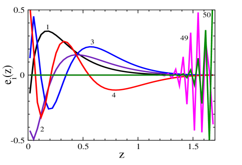
Principal components have one distinct advantage over fixed parametrizations. They allow the data to determine which weight of the cosmological function $w(z)$ (or $\rho_{\rm DE}(z)$, or $H(z)$) is best determined. In fact, the PCs depend on the cosmological probe, on the specifications of the probe (redshift and sky coverage etc), and (more weakly) on the true cosmological model. These dependencies are features and not bugs, and they make the principal components a useful tool in survey design. For example, one can design a survey that is most sensitive to the dark energy equation of state at some specific redshift, or study how many independent parameters are measured by any given combination of cosmological probes (e.g. Linder_howmany ).

II.4 Uncorrelated estimates of DE evolution

A useful extension of the principal component formalism is to compute the band powers in redshift of the dark energy function, $w(z)$ (or $\rho_{\rm DE}(z)$ or $H(z)$). These band powers can be made 100% uncorrelated by construction, and the price to pay is a small leakage in the sensitivity of each band power outside of its redshift range. For details on how this is implemented, see Huterer_Cooray .

Figure 3: Top panel: constraints on the four band powers of $w(z)$, adopted from Ref. Huterer_Cooray , assuming the Riess04 SNa data Riess_04 and a prior on $\Omega_{M}$. Bottom panel: the same method applied to constrain three band powers, using the newest data SNa Ia data from the Hubble Space Telescope (adopted from Ref. Riess_06 ) in combination with the baryon acoustic oscillation measurements BAO .

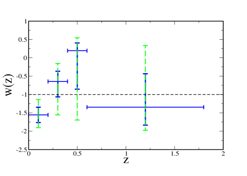
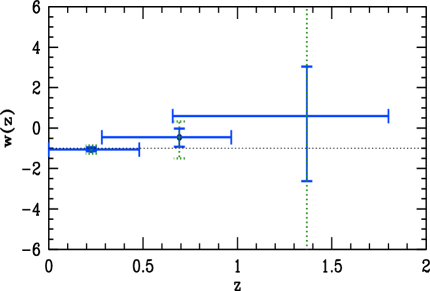
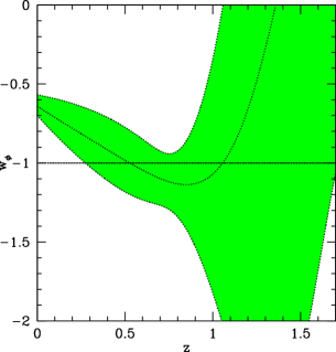
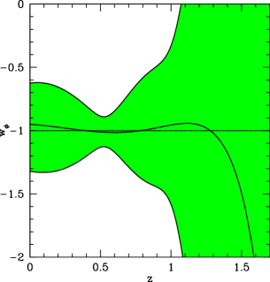
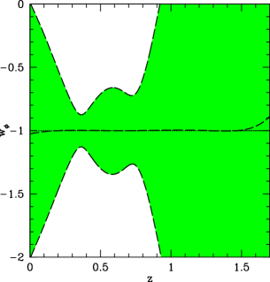
The top panel of Figure 3 shows the constraints on the four band powers of $w(z)$, adopted from Ref. Huterer_Cooray , assuming the Riess04 SNa data Riess_04 and a prior on $\Omega_{M}$. The bottom panel of the Figure shows the same method to constrain three band powers, using the newest data SNa Ia data from the Hubble Space Telescope, adopted from Ref. Riess_06 , in combination with the baryon acoustic oscillation measurements BAO .. The slight preference for $w(z)$ increasing with redshift is seen in both panels; however, significant systematics still affect the data, in particular because of the heterogeneity of the SNa Ia datasets used. Therefore, it is too early to claim any evidence for the departures from $\Lambda$CDM , and it remains to be seen how the results change once we have a systematically more homogeneous and statistically more powerful data set (for the requirements on the SNa Ia systematics, see Kim_Linder ).

It interesting to see in Fig. 3 how good the constraints are, given that this is current data and that interesting constraints are obtained on 3-4 band powers. A superior data set with an excellent control of the systematics, such as that expected from a dedicated space telescope such as SuperNova/Acceleration Probe (SNAP; SNAP ) will significantly improve the constraints, and also allow a finer resolution (i.e. more band power parameters) in redshift.

Nevertheless, it is clear from the existing set that either significant redshift evolution in $w$ or significant improvement in the data will be required before either redshift evolution or deviation from $-1$ could be unambiguously inferred using this technique. We now turn to considering this question in more detail

III Lambda or not?

As stressed earlier, one of the most important outstanding questions in cosmology is whether dark energy is consistent with a cosmological constant. This hypothesis can be tested in a variety of ways. The simplest approach is to compute a simple likelihood comparison between the data and the vacuum energy model $w(z)=-1$. A much more sophisticated (but admittedly less robust) approach would be to perform some type of reconstruction of the energy density $\rho_{\rm DE}(z)$ and check whether or not it is consistent with a constant value (or similarly, to reconstruct the equation of state $w(z)$ and check whether it is consistent with $-1$).

Here we consider the $\Lambda$ hypothesis test in terms of principal components (PCs). We consider models in the $w_{0}$-$w_{a}$ plane (see Eq. (4)) and as we outline below, we use the best measured PCs to determine if we can statistically distinguish distinguish the model from $\Lambda$CDM . In this section, we assume future SNa Ia data with 3000 SNe distributed uniformly in $0.1<z<1.7$; this corresponds roughly (but not exactly) to what is expected from the SNAP space telescope SNAP .

For a fixed dark energy model described by some values of the cosmological parameters $w_{0}$ and $w_{a}$, let the principal components take values $\alpha_{i}$, with associated errors $\sigma(\alpha_{i})$ (note, we marginalize the results over the values of $\Omega_{M}$, thus enlarging the errors in the PCs; in this way we can talk about models in the $w_{0}$-$w_{a}$ plane without further recourse to $\Omega_{M}$). Further, from Eq. (10) it follows that the principal component coefficients for the $w(z)=-1$ model are

$$\bar{\alpha_{i}}=(-1)\,\sum_{a=1}^{N}e_{i}(z_{a}),$$ (11)

where $e_{i}(z)$ is the shape of $i$th PC in redshift. We can now perform a simple $\chi^{2}$ test to determine whether $w$ is constant:

$$\chi^{2}=\sum_{i=1}^{M}{(\alpha_{i}-\bar{\alpha_{i}})^{2}\over\sigma^{2}(\alpha_{i})},$$ (12)

where we have chosen to keep only the first $M$ PCs, since the best-determined modes will contribute the most to the sum (note that the test is valid regardless of the value of $M$; in practice, our M is typically 3-5). Given that we have $M$ degrees of freedom, each model $(w_{0},w_{a})$ will lead to $\chi^{2}$ which may or may be inconsistent with the $\Lambda$CDM model at some fixed confidence level.

In order to determine the ability of future SN surveys to make this distinction, we focus here on the sensitivity of the results to the measured magnitude uncertainty. We focus on this factor for two reason. First, we believe it will be the single most important determinant of the ability of future surveys to possibly rule out a cosmological constant, and second, because our examination of past surveys suggests that one should consider the possibility of redshfit-dependent magnitude measurement errors. This latter possibility is not unexpected. It is systematically harder to determine the luminosity of ever fainter and more distant objects.

Indeed, it is this possibility that originally motivated kraussdavislinton the current study. Measuring supernovae at ever higher redshift provide a useful lever-arm to distinguish between different equations of state, unless the magnitude uncertainty increases more quickly with redshift than the redshift-distance relation diverges for differing values of the dark energy equation of state. For purposes of this example analysis, we used 217 SN1a, from the initial large SN surveys Perlmutter_99 ; Riess_98 , supplemented by several more recent measurements, fitting the quoted magnitude uncertainty as a function of redshift to a linear relation. Although the oft-claimed quoted magnitude uncertainty per low-redshift supernova is $0.15$ we found that a free fit to the data tended to prefer a slightly larger value. Thus, for purposes of comparison, we considered both redshift independent uncertainties of $0.15$ or $0.21$ magnitudes, as well as redshift dependent uncertainties $0.15+0.079z$ or $0.21+0.079z$ mag.

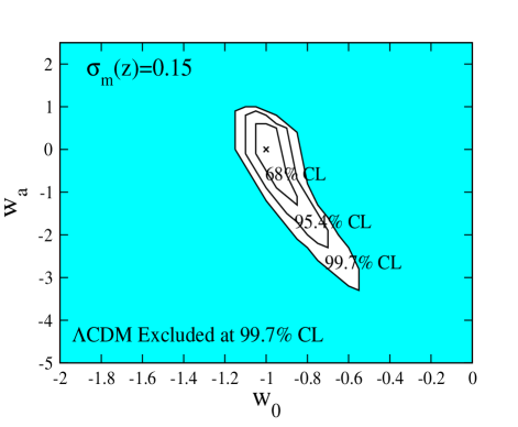
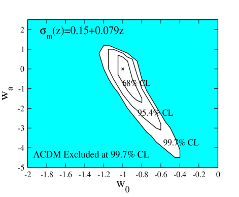
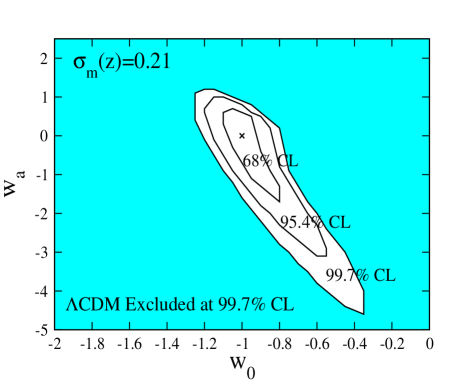
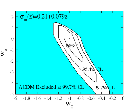
Figure 4, shows the regions in the $w_{0}-w_{a}$ that are ruled out at 68% C.L. (region outside of the innermost closed curve) 95% C.L. (region outside of the middle curve) and 99.7% C.L. (region outside of the outermost curve, coinciding with the blue shaded region). In other words, the blue region corresponds to dark energy scenarios where the $\Lambda$CDM model can be ruled out at $>3\sigma$ confidence.

In the four panels of Figure 4 we show cases when the error per SNa is $0.15$ or $0.21$ magnitudes, and when it is increasing with redshift as $0.15+0.079z$ or $0.21+0.079z$ mag. Clearly, increasing magnitude uncertainties with redshift can significantly affect the size of the indistinguishable parts of model space. Note too that the shape of the region that cannot be distinguished from $\Lambda$CDM is of characteristic shape, is elongated roughly along the $7(w_{0}+1)+w_{a}\approx 0$ direction — this is a direct consequence of the fact that the physically relevant quantity is $w(z)=w_{0}+w_{a}z/(1+z)$.

Figure 4: Regions in the $w_{0}-w_{a}$ that are ruled out at 68% C.L. (region outside of the innermost closed curve) 95% C.L. (region outside of the middle curve) and 99.7% C.L. (region outside of the outermost curve, coinciding with the blue shaded region). In other words, the blue region corresponds to dark energy scenarios where the $\Lambda$CDM model can be ruled out at $>3\sigma$ confidence. This test is performed by “measuring” the principal components from each $(w_{0},w_{a})$ model and comparing them to those from the $\Lambda$CDM model. We show cases when the error per SNa is $0.15$ or $0.21$ magnitudes (top and bottom left panels), and when it is increasing with redshift as $0.15+0.079z$ or $0.21+0.079z$ mag (top and bottom right panels).

One other way to get a handle on whether $w\neq-1$ is to explore the most precise constraint on $w$ that might be obtainable at any single redshift. For, if $w\neq-1$ at any redshift, this will establish unambiguously that the dark energy is not a cosmological constant.

To explore the sensitivity of SNe for this purpose we parametrize dark energy equation of state as in Eq. (4), and study the accuracy in the equation of state $w(z)$ at the best determined, or pivot, point. The pivot value is given by Huterer_Turner ; DETF

$$w_{\rm pivot}=w_{0}-{{\rm Cov(w_{0},w_{a})}\over{\rm Cov(w_{a},w_{a})}}\,w_{a}$$ (13)

where ${\rm Cov}(x,y)$ stands for elements of the covariance matrix element, while the pivot redshift at which $w(z)$ is best determined is given by

$$z_{\rm pivot}=-{{\rm Cov(w_{0},w_{a})}\over{\rm Cov(w_{0},w_{a})}+{\rm Cov(w_{a},w_{a})}}.$$ (14)

Other parameter we are the matter density relative to critical, $\Omega_{M}$ and the offset in the SNa Ia Hubble diagram, $\mathcal{M}$. Throughout we assume a flat universe.

Figure 5: Constraints on the pivot value of the equation of state, $w_{\rm pivot}$, as a function of the intercept and slope of the magnitude error of SNe, $\sigma_{m}(0)$ and $A$. We have assumed a fiducial survey of 2800 SNe.

Using a Fisher matrix formalism, we estimate errors for a future SNAP-type survey SNAP with 2800 SNe distributed in redshift out to $z=1.7$ as given by SNAP , and combined with 300 local supernovae uniformly distributed in the $z=0.03-0.08$ range. We study how the errors of the parameter of most interest, $w_{\rm pivot}$, change as the individual SNa errors vary. We again assume that the statistical error per SNa scales with redshift as

$$\sigma_{m}(z)=\sigma_{m}(0)+Az,$$ (15)

where $\sigma_{m}(0)=0.10$, $0.15$ or $0.20$, and we now let $A$ vary in order to ascertain sensitivity to this parameter

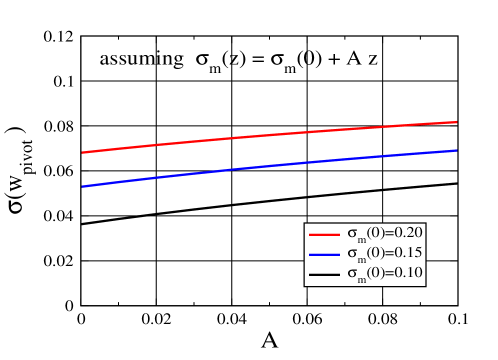
As can be seen in Fig. 5, the constraints on $w_{\rm pivot}$ are dependent on both $\sigma_{m}(0)$ and $A$; we can fit the constraint via an approximate relation

$$\sigma(w_{\rm pivot})\approx 0.17\,(2\sigma_{m}(0)+A).$$ (16)

This equation shows that the slope of the statistical error vs. redshift relation, $A$, contributes to $\sigma(w_{\rm pivot})$ one half as much as the intercept of the same relation, $\sigma_{m}(0)$. For example, a 20% increase in the SNa error between the redshift of 0 and 1 (so that $A=0.2\sigma_{m}(0)$) will lead to a 10% increase in error associated with the pivot value of the equation of state.

IV Conclusions

SNe Ia are currently the strongest cosmological probes of dark energy, and are likely to remain the most solid source of information in the near future. This implies that control of the statistical errors is crucial. In particular, if we are ever to address the central question of cosmology, ’Is the dark energy due to a cosmological constant?’, we need to be able to unambiguously determine that $w\neq-1$ at some, or all redshifts. The extent to which SNe Ia measurements will allow such a determination has been our prime concern in this analysis

Figures 4 and 5 represent our primary results in this regard. Figure 4 makes clear that the model-independent constraints on $w(z)$, for a two-parameter class of deviations around $w(z)=-1$ (the two parameters are $w_{0}$ and $w_{a}$; see Eq. (4)), are quite sensitive to the measurement uncertainty in supernova magnitudes. Moreover, both Figure 4 and Fig. 5 demonstrate that it is particularly important to attempt to maintain control over measurement uncertainties for higher redshift supernovae. As Figure 4 also demonstrates, allowing for possible variations in $w$ with redshift implies to reduce the $95\%$ confidence limit uncertainty in $w(z)$ for a fit near $w_{0}=-1$ and $w_{a}=0$ significantly below 10 $\%$ in $w_{0}$ will be challenging.

This latter point is even more important when considering whether one might utilize the measured value of $w(z)$ at the pivot point to attempt to discern some time at which $w\neq-1$. Redshift-dependent uncertainties in supernova magnitudes can easily almost double the inferred uncertainty in $w$ at this point. Moreover, only if the planned large scale SNe surveys can maintain a uniform magnitude uncertainty per supernova, $\sigma_{m}$, less than $0.10$ can we hope to derive a $95\%$ confidence limit uncertainty in $w_{\rm pivot}$ of less than about $10\%$ (see Fig. 5) which itself may not be sufficient to distinguish some non-standard dark energy models from a cosmological constant.

It is not clear whether resolving the nature of dark energy is a 10-year or a 100-year problem. The answer partly depends on how much information measurements of dark energy can provide. Here we have addressed the former problem by studying the requirements of magnitude errors in a SNa Ia survey. Our results may be viewed as discouraging, or they may be viewed as inspiring for those observers who enjoy a demanding challenge. It is already becoming clear that, in order to have hope of detecting a deviation from the cosmological constant scenario, we need nature to be kind by producing a non-negligible deviation in $w(z)$ at some redshift, and we need to control SNa magnitude errors, and systematics in particular, to high precision. If either one of these requirements is not met, may have to rely on theorists to understand the nature of dark energy, which is option over which we may have much less control.

References

- (1) A. Riess et al., Astron. J. 116, 1009 (1998)
- (2) S. Perlmutter et al., Astrophys. J. 517, 565 (1999)
- (3) L. Krauss and M. S. Turner, Gen. Rel. Grav. 27, 1137 (1995)
- (4) D. Spergel et al., Astrophys. J. Suppl. 148, 175 (2003); D. Spergel et al., astro-ph/0603449
- (5) M. Tegmark et al, Phys. Rev. D 69, 103501 (2004)
- (6) D.J. Eisenstein et al, Astrophys. J. 633, 560 (2005).
- (7) A. Riess et al., Astron. J. 607, 665 (2004)
- (8) R.A. Knop et al., Astron. J. 598, 102 (2003)
- (9) P. Astier et al., Astron. Astrophys. 447, 31 (2006)
- (10) A. Riess et al., astro-ph/0611572.
- (11) W.M. Wood-Vasey et al, astro-ph/0701041.
- (12) C. Wetterich, Nucl. Phys. B 302, 668 (1988)
- (13) K. Freese et al., Nucl. Phys. B 287, 797 (1987)
- (14) B. Ratra and P. J. E. Peebles, Phys. Rev. D 37, 3406 (1988)
- (15) K. Coble, S. Dodelson, and J. Frieman, Phys. Rev. D 55, 1851 (1996).
- (16) P. G. Ferreira and M. Joyce, Phys. Rev. D 58, 023503 (1998).
- (17) R. Caldwell, R. Dave, and P. J. Steinhardt, Phys. Rev. Lett. 80, 1582 (1998).
- (18) A. R. Cooray and D. Huterer, Astrophys. J., 513, L95 (1999)
- (19) E.V. Linder, Phys. Rev. Lett. 90 091301 (2003).
- (20) B.A. Bassett, M. Kunz, J. Silk and C. Ungarelli, MNRAS, 336, 1217 (2002).
- (21) P.S. Corasaniti and E.J. Copeland, Phys. Rev. D 65 043004 (2002);
- (22) E.V. Linder and D. Huterer, Phys. Rev. D 72, 043509 (2005).
- (23) T.D. Saini, S. Raychaudhury, V. Sahni and A. Starobinsky, Phys. Rev. Lett. 85, 1162 (2000).
- (24) V. Sahni, T.D. Saini, A. Starobinsky and U. Alam, JETP Lett. 77, 201 (2003); U. Alam, V. Sahni, T.D. Saini and A. Starobinsky, MNRAS, 344, 1057 (2003).
- (25) D. Huterer and M. S. Turner, Phys. Rev. D 60, 081301 (1999)
- (26) T. Nakamura and T. Chiba, Mon. Not. R. astron. Soc. 306, 696 (1999)
- (27) A.A. Starobinsky, JETP Lett. 68, 757 (1998)
- (28) J. Weller and A. Albrecht, Phys. Rev. D 65, 103512 (2002).
- (29) D. Huterer and M. S. Turner, Phys. Rev. D 64, 123527 (2001).
- (30) G. Zhao, J. Xia, B. Feng and X. Zhang, 2006, astro-ph/0603621; J. Xia, G. Zhao, H. Li, B. Feng and X. Zhang, Phys. Rev. D 74, 083521 (2006).
- (31) V. Sahni and A. Starobinsky, astro-ph/0610026.
- (32) D. Huterer and G.D. Starkman, Phys. Rev. Lett. 90, 031301 (2003).
- (33) R.G. Crittenden and L. Pogosian, astro-ph/0510293
- (34) F. Simpson and S. Bridle, Phys. Rev. D, 73, 083001 (2006).
- (35) A.J.S. Hamilton and M. Tegmark, MNRAS, 312, 285 (2000); M. Tegmark, Phys. Rev. D, 55, 5895 (1997).
-
(36)
SNAP – http://snap.lbl.gov ;
G. Aldering et al. 2004, astro-ph/0405232 - (37) D. Huterer and A. Cooray, Phys. Rev. D 71, 023506 (2005).
- (38) A. Kim, E.V. Linder, R. Miquel, and N. Mostek, N., MNRAS 347, 909 (2004)
- (39) A. Albrecht et al, Dark Energy Task Force Report [astro-ph/0609591].
- (40) E. Linton, C. Davis, and N. Borchers, 2001-2005 CWRU senior projects with L. Krauss.