The N/O evolution on galaxies:
the role played by the star formation history

Abstract

We study the evolution of nitrogen resulting from a set of spiral and irregular galaxy models computed for a large number of input mass radial distributions and with various star formation efficiencies. We show that our models produce a nitrogen abundance evolution in good agreement with the observational data. In particular, low N/O values for high-redshift objects, such as those obtained for Damped Lyman Alpha galaxies can be obtained with our models simultaneously to higher and constant values of N/O as those observed for irregular and dwarf galaxies, at the same low oxygen abundances $\rm 12+log(O/H)\sim 7$ dex. The differences in the star formation histories of the regions and galaxies modeled are essential to reproduce the observational data in the N/O-O/H plane.

1 The plane N/O vs O/H

The whole set of data in the plane N/O-O/H (for references od data see Table 1 from [Mollá et al.(2006)]), such as they are shown in Fig. 1, are limited by three possible theoretical lines:

1. the line defined by the secondary nitrogen behavior, NS, when N needs a seed of O to be created.

2. the corresponding one for primary nitrogen, NP, when N is created directly from H or He for any oxygen abundance

3. NS+NP when both contributions there exist

It is evident that a primary N contribution must exist. Actually, a secondary production of N is expected for most stars as corresponds to a CNO cycle, but it is well established that a primary production should arise from intermediate mass stars ($\rm 4\leq M<8M_{\odot}$) that suffer dredge-up and hot-bottom burning episodes during the asymptotic giant branch ([Renzini & Voli 1981, van den Hoek & Groenewegen 1997]).

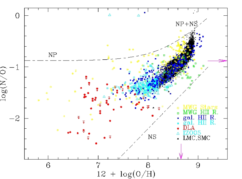
Figure 1: The relative abundance $log(N/O)$ vs the oxygen abundance $12+log(O/H)$ observations. Black small points are the SDSS galaxy data from [Liang et al.(2006)]. Yellow open dots are data for Galactic stars. The green open, solid blue and cyan squares are the Hii region data for MWG, metal-rich and metal-poor galaxies, respectively, (including in the last ones data from [Nava et al. 2006] and [Izotov & Thuan 1999, Izotov et al. 2006] estimates). The large cyan open triangle is lowest galaxy known data, given by [Izotov, Thuan & Guseva(2005)]. Red fill dots are values for Damped Lyman Alpha objects.

2 The evolution of nitrogen in the Milky Way Galaxy

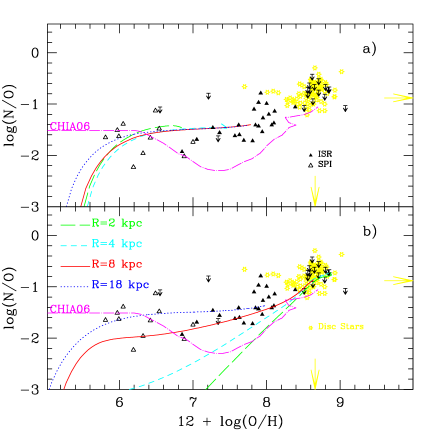
Figure 2: The evolution of the relative abundance $log(N/O)$ vs the oxygen abundance $12+log(O/H)$ for four regions of MWG located at galactocentric distances $R=2$,4, 8 and 18 kpc as labelled. Upper panel for the halo regions. Bottom panel for the disc regions. The data correspond to Galactic stars of the halo (black triangles) and of the disc (yellow open dots).

Using massive star yields from [Woosley & Weaver (1995)] and low and intermediate star yields from [Gavilán, Buell & Mollá (2005)] with a certain proportion of primary N, dependent on metallicity, a Galactic chemical evolution model (GCEM) has been calculated ([Gavilán, Mollá & Buell 2006]) which reproduces most data of the Milky Way Galaxy (MWG). In Fig. 2 the MWG model results are shown separately for the halo (a) and for the disk (b). In each panel the evolution for four regions, located at different distance of the galaxy center are represented. The evolution in the halo is similar for all regions, reaching the level observed of relative abundance N/O and maintaining an almost constant ratio. This behavior is in agreement with the observed trend for the halo stars, in particular the recent ones from [Israelian et al. (2004)] and from [Spite et al. (2005)]. In the disk, however, each radial region has its own evolution, as corresponds to the different star formation history that occurs in each one. The outer regions with quiet star formation histories have still low oxygen abundances when the intermediate stars begin to eject their primary nitrogen, while the inner regions, that suffer a strong and early star formation rate, have created many generations of stars, ans consequently produced high oxygen abundances before this NP appears in the interstellar medium. For $R=2$ or 4 kpc this NP appears at almost solar oxygen abundances, shown in the figure like a smoother increase or even as a flattening of the evolutionary track. For comparison purposes we also draw the Solar region model from [Chiappini et al.(2006)] where NP proceeds from low Z massive stars rotating at very high velocity. Our model reproduces better the observations.

3 The results of our simulations for all time steps

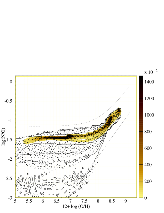
Figure 3: The relation between N/O and O/H for the simulated galaxies. The complete results for all modeled regions shown as small dots. Colored contours represent the isolines of number of points included within them (see relative scale to the right), while solid lines represent the regions with 0.3, 0.03, 0.012 and 0.003 %, respectively, of the total number of points. The data region is limited by the two dashed lines.

Since these stellar yields seem to be good enough to fit the Galactic data we apply them to a wide grid of theoretical galaxies with different total mass ([Mollá & Díaz 2005]). Using different star formation rate efficiencies, we obtain different results of abundances for the whole set of models. For details, see [Mollá et al.(2006)]. In Fig. 3 we show the results, for all calculated times and models, as small dots. Over them we have plot some contours in yellow levels. Furthermore, we draw some other contours as solid lines for regions with 0.3, 0.03, 0.012 and 0.003 %, respectively, of the total number of points. The model results for all time step is also in agreement with the observed trends showing:

• The low mass galaxies maintain a flat behavior in the plane N/O-O/H with an almost constant abundance N/O even for oxygen abundances as low as $12+log(O/H)\sim 6.5-7$

• The massive galaxies show a different trend in that plane depending on their star formation history. The most efficient in forming stars, that is those that create them by mean of a high and early star formation rate, seem to have a secondary behavior from the first moment with a very steep evolution of N/O vs O/H.

• This behavior behaves more like primary+secondary, that is with a smaller slope in that graph, when stars form less efficiently reaching the primary line of low mass galaxies when the star formation rate is very low. These simulated galaxies would appear as low brightness massive galaxies.

• The predicted dispersion is also large, as shown by the observations.

4 The present time abundances for a grid of models

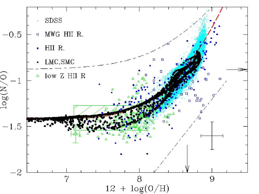
Figure 4: The relative abundance $log(N/O)$ vs the oxygen abundance $12+log(O/H)$ resulting from our models for the present time as full black dots compared with the data corresponding to Galactic and extragalactic Hii regions of SDSS galaxies ([Liang et al.(2006)], small cyan and green points for metal-rich and metal-poor galaxies), to galactic and extragalactic Hii regions from authors of Table 1 of [Mollá et al.(2006)] (blue open and full squares, respectively), and for low metallicity galaxies ([Nava et al. 2006, Izotov & Thuan 1999, Izotov et al. 2006] as green triangles). The long-dashed line is the least squares fitting function to models. The large triangle around $12+log(O/H)\sim 7.1$ is the value found by [Izotov, Thuan & Guseva(2005)] for the lowest-metallicity star-forming galaxy known.

We represent the present time model results in the plane N/O vs O/H in Fig. 4 as small black points, that we compared with the galactic and extragalactic Hii regions data. The models are fitted by a least-squares polynomial function:

$$log(N/O) = -1149.31+1115.23x-438.87x^{2}+90.05x^{3}$$

$$-10.20x^{4}+0.61x^{5}-0.015x^{6}$$

where $x=12+log(O/H)$.

We demonstrate that using yields from LIM mass stars and a model with star formation efficiencies variable for each galaxy, we may obtain points in the plane N/O-O/H in agreement with data, even for what refers to the observed dispersion which also may partially be simulated with our models. In the figure we have plot a shaded rectangle showing the region where abundances N/O fall within a Gaussian distribution, which implies that differences shown by points in this zone with models may be mainly imputed to observational errors ([Nava et al. 2006]).

5 The time or redshift evolution of N/O

Figure 5: The relation N/O – O/H for different evolutionary times: $\rm t=0.1$, $\rm t=0.17$, $\rm t=0.30$, and $\rm t=13.2$ Gyr, as marked in the figure. Data as full dots or triangle correspond to DLA objects.

Finally, in order to explore the time evolution of the modeled abundances, we show in Fig. 5 the results for four different time steps: $\rm t=0.1$, $\rm t=0.17$, $\rm t=0.30$, and $\rm t=13.2$ Gyr. These epochs would correspond to redshifts z$\sim$3.8, 3.7, 3.5, and 0, respectively, for a cosmology with H${}_{0}=71$, $\Omega_{M}=0.30$, $\Omega_{\Lambda}=0.70$, if the formation of these spiral and irregular galaxies occurred at a redshift z$\sim 4$. A large gap appears between the results for each one of our time steps. In particular, our models predict a feature similar to the so-called second plateau which Centurión et al. (2003) claim to exist at a metallicity around $\rm 12+log(O/H)\sim 7$, which appears at a level of $\rm\log{(N/O)}\sim-2.3$ for $\rm 12+log(O/H)\sim 6.5-7$, while most points appear at a higher level of N/O ($\geq-1.8$) for a similarly low O/H abundance. In fact, no gap is apparent between models at 1.1 and 13.2 Gyr, thus making it difficult to discriminate objects at a redshift up to $z<2.5$ from those at redshift z=0 in the N/O-O/H plane, as it is actually the case. The abundances predicted for galaxies at redshift $z\geq 3.$ are far enough from the rest of the points in the plot so as to disentangle them from a given data sample.

6 Concluding remarks

These results are only partially due to the dependence with metallicity of the yields we use. This contribution of primary N, larger for low metallicity stars than for high metallicity ones, is important since it allows to us to obtain tracks in the plane N/O vs O/H flatter than the ones predicted with a constant contribution of the primary N. We must to do clear, however, that if we eliminate the metallicity dependence from the yields, we still obtain different tracks for regions with different star formation histories, such as we demonstrate with detail [Mollá et al.(2006)].

The absolute level of observations and the fine tuning of the observed shape in the plane N/O-O/H for the present time data, however, is only reproduced if the stellar yields, in turn, give the right level of primary nitrogen and have the adequate dependence on metallicity. The chemical evolution models must also be well calibrated in order to predict star formation histories able to produce abundances in agreement with data. Therefore, the adequate selection of metallicity dependent LIM star yields joined to the accurate chemical evolution models are able to predict abundances for N and O which reproduce the complete set of data in the plane N/O vs O/H.

The main outcomes of this work are the following:

• The evolutionary track of a region or galaxy in the plane N/O-O/H is very dependent on the star formation history. When this occurs as a strong burst the evolution follows a secondary behavior while a continuous, quiet and low star formation rate gives a flat slope in that plane.

• Intermediate star formation histories are between the two referenced extreme trends, producing this way a large dispersion of the corresponding data which is similar to the observed one

• The final points of our realizations, corresponding to the present time abundances, reproduce very well the trend given by Hii regions data.

• The trend given by low-metallicity data from the MWG halo is also well fitted.

• The data proceeding from high-redshift objects may be easily explained with the abundances calculated for other evolutionary times. In particular something like a second plateau appears when results for $z>3$ are plotted.

References

- [Chiappini et al.(2006)] Chiappini C., Hirschi R., Matteucci F., Meynet G., Ekstrom S., Maeder A., 2006, astro, arXiv:astro-ph/0609410
- [Gavilán, Buell & Mollá (2005)] Gavilán M., Buell J. F., Mollá M., 2005, A&A, 432, 861
- [Gavilán, Mollá & Buell 2006] Gavilán M., Mollá M., Buell J. F., 2006, A&A, 450, 509
- [Israelian et al. (2004)] Israelian G., Ecuvillon A., Rebolo R., García-López R., Bonifacio P., Molaro P., 2004, A&A, 421, 649
- [Izotov et al. 2006] Izotov Y. I., Stasińska G., Meynet G., Guseva N. G., Thuan T. X., 2006, A&A, 448, 955
- [Izotov, Thuan & Guseva(2005)] Izotov Y. I., Thuan T. X., Guseva N. G., 2005, ApJ,2,2
- [Izotov & Thuan 1999] Izotov Y. I., Thuan T. X., 1999, ApJ, 511, 639
- [Liang et al.(2006)] Liang Y. C., Yin S. Y., Hammer F., Deng L. C., Flores H., Zhang B., 2006, ApJ, 652, 257
- [Mollá & Díaz 2005] Mollá M., Díaz A. I., 2005, MNRAS, 358, 521
- [Mollá et al.(2006)] Mollá M., Vílchez J. M., Gavilán M., Díaz A. I., 2006, MNRAS, 372, 1069
- [Nava et al. 2006] Nava A., Casebeer D., Henry R. B. C., Jevremovic D., 2006, ApJ, 645, 1076
- [Renzini & Voli 1981] Renzini A., Voli M., 1981, A&A, 94, 175
- [Spite et al. (2005)] Spite M., Cayrel R., Plez B., Hill V., Spite F., Depagne E., François P., Bonifacio P., Barbuy B., Beers T., Andersen J., Molaro P., Nordström B., Primas F., 2005, A&A, 430, 655
- [van den Hoek & Groenewegen 1997] van den Hoek, L. B. & Groenewegen, M. A. T. 1997, A&AS, 123, 305
- [Woosley & Weaver (1995)] Woosley S. E., Weaver T. A., 1995, ApJS, 101, 181