Photospheric magnetic field and chromospheric emission

Abstract

We present a statistical analysis of network and internetwork properties in the photosphere and the chromosphere. For the first time we simultaneously observed (a) the four Stokes parameters of the photospheric iron line pair at 630.2 nm and (b) the intensity profile of the Ca H line at 396.8 nm. The vector magnetic field was inferred from the inversion of the iron lines. We aim at an understanding of the coupling between photospheric magnetic field and chromospheric emission.

1 Observations and data reduction

We observed a series of 13 maps of a network region and the surrounding quiet Sun at a heliocentric angle of 53^∘, close to the active region NOAA 10675 on September 27, 2004, with POLIS (Schmidt et al., 2003; Beck et al., 2005) at the German VTT in Tenerife. The Kiepenheuer Adaptive Optics System (KAOS) was used to improve spatial resolution to about 1 arcsec (von der Lühe et al., 2003).

Using  the average profile  of each map, we normalized  the intensity at the line wing at    396.490 nm to the FTS profile (Stenflo et al., 1984). ¿From the intensity profile of Ca H we define line properties like, e.g., the H-index, which is the integral around the line core from 396.8 nm to 396.9 nm. The separation between network and internetwork is based on (i) the maps of magnetic flux density, (ii) the presence of Stokes-$V$ signals and emission in Ca H.

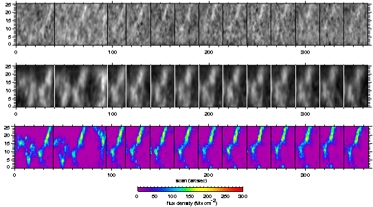
Figure 1: Top to buttom: the continuum intensity close to 630 nm, the H-index, and the magnetic flux density obtained from the inversion.

2 Inversion

An inversion was performed for the two iron lines at 630 nm using the SIR code (Ruiz Cobo & del Toro Iniesta 1992). To mimic unresolved magnetic fields, we used a model atmosphere with one magnetic and one field-free component, plus stray light. The inversion yields a magnetic field vector, a line-of-sight velocity, and the magnetic flux per pixel. These quantities are constant along the line of sight. Using the flux density maps, we created a mask to separate network and internetwork regions.

Figure 2: Distribution of the magnetic field strength for the network (thick) and internetwork (thin).

3 Magnetic field distribution

The polarization signal in $Q(\lambda)$, $U(\lambda)$, and $V(\lambda)$ is normalized by the local continuum intensity, $I_{c}$, for each pixel. The rms noise level of the Stokes parameters in the continuum was $\sigma$ = 8.0 $\times 10^{-4}$ $I_{c}$ for the Fe I 630 nm lines. Only pixels with $V$ signals greater than 3 $\sigma$ were included in the profile analysis. We obtain a magnetic field distribution which peaks at some 1.4 kG for the network elements and at about 200 G for the internetwork elements in agreement with previous infrared observations, but in contradiction with results from visible lines (Collados, 2001; Lites, 2002).

3.1 The effect of noise in the weak-field limit

Our finding of weak rather than strong fields can be explained by the high spatial resolution and high polarimetric accuracy that we have achieved in our measurements. Since the internetwork magnetic fields are in the weak-field limit, the amount of noise strongly influences the outcome of the inversion. Figure 3 shows two different cases:

1. A fit of an original set of Stokes profiles yields $B$ = 840 G with a filling factor of 7.6 % (left panel, Fig. 3).

2. A fit on the same profile with added noise (such that the rms noise level is twice as large) delivers $B$ = 1.5 kG and a filling factor of only 5.3 % (right four panels, Fig. 3).

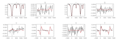
Figure 3: The left (right) four panels show the inversion results of the original (noisy) data.

The reduction of noise and improvement of spatial resolution may resolve the existing discrepancy between visible and infrared magnetic field measurements.

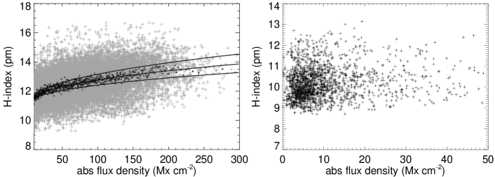
Figure 4: The H-index vs. the magnetic flux density in the network (left) and internetwork (right). Black squares show the binned data. The curves show the fit to the original data along with 1 $\sigma$ confidence level.

4 The H-index vs. magnetic flux density

The left panel of Fig. 4 shows the H-index versus photospheric magnetic flux, $\Phi$, for the network. A power law fit, $H=a\,\,\Phi^{b}+c$, yields $b$ = 0.3 and $c$ = 10 pm. In the internetwork the H-index does not correlate with the magnetic flux density (Fig. 4, right panel). The average value of the H-index in the internetwork is about $H$ = 10 pm. The offset value, $c$ = 10 pm, can be interpreted as the non-magnetic heating contribution and the stray light.

For the first time the H-index and simulaneously measured V-profile parameters can be compared. We find no correlation between these parameters in the internetwork (Fig. 5, pluses). In the network, a correlation exists, and the H-index peaks at a small positive value for the area asymmetry and at vanishing V-profile Doppler shift (Fig. 5, squares).

5 Conclusions

$\bullet$ The internetwork magnetic field distribution peaks around 200 G and its mean absolute flux density amounts to 9 Mx cm^-2. The finding of weak rather than strong fields is a consequence of the high spatial resolution and high polarimetric accuracy.

$\bullet$ The H-index in the network is correlated to the magnetic flux density, approaching a value of $H$ = 10 pm for vanishing flux.

$\bullet$ The H-index in the internetwork is not correlated to any property of the photospheric magnetic field implying that the chromospheric brightenings in the internetwork are non-magnetic.

$\bullet$ For high values of the H-index, the network shows small positive area (and amplitude) asymmetry, being consistent with the scenario of a line-of-sight crossing the magnetic boundary (canopy) of flux tubes that fans out with height (Steiner, 1999).

Figure 5: Scatter plot of the area asymmetry and Stokes-$V$ velocity against the H-index.

References

- Beck et al. (2005) Beck, C., Schlichenmaier, R., Collados, M., Bellot Rubio, L., & Kentischer, T. 2005, A&A, 443, 1047
- Collados (2001) Collados, M. 2001, in ASP Conf. Ser. 236: Advanced Solar Polarimetry – Theory, Observation, and Instrumentation, ed. M. Sigwarth, 255
- Lites (2002) Lites, B. W. 2002, ApJ, 573, 431
- Ruiz Cobo & del Toro Iniesta (1992) Ruiz Cobo, B. & del Toro Iniesta, J. C. 1992, ApJ, 398, 375
- Schmidt et al. (2003) Schmidt, W., Beck, C., Kentischer, T., Elmore, D., & Lites, B. 2003, Astronomische Nachrichten, 324, 300
- Steiner (1999) Steiner, O. 1999, in ASP Conf. Ser. 184: Third Advances in Solar Physics Euroconference: Magnetic Fields and Oscillations, 38–54
- Stenflo et al. (1984) Stenflo, J. O., Solanki, S., Harvey, J. W., & Brault, J. W. 1984, A&A, 131, 333
- von der Lühe et al. (2003) von der Lühe, O., Soltau, D., Berkefeld, T., & Schelenz, T. 2003, in Innovative Telescopes and Instrumentation for Solar Astrophysics. Proceedings of the SPIE, Volume 4853, ed. S. L. Keil & S. V. Avakyan, 187–193